Characterizing the $\gamma$-Ray Variability of Active Galactic Nuclei with Stochastic Process Method

Abstract

The $\gamma$-ray astronomy in time domain has been by now progressed further as the variabilities of Active Galactic Nuclei (AGNs) on different timescales have been reported a lot. We study the $\gamma$-ray variabilities of 23 jetted AGNs through applying a stochastic process method to the $\sim$12.7 yr long-term light curve (LC) obtained by Fermi-Large Area Telescope (Fermi-LAT). In this method, the stochastically driven damped simple harmonic oscillator (SHO) and the damped random walk (DRW) models are used to model the long-term LCs. Our results show that the long-term variabilities of 23 AGNs can be characterized well by both SHO and DRW models. However, the SHO model is restricted in the over-damped mode and the parameters are poorly constrained. The SHO power spectral densities (PSDs) are same as the typical DRW PSD. In the plot of the rest-frame timescale that corresponds to the broken frequency in the PSD versus black hole mass, the intrinsic $\gamma$-ray characteristic timescales of 23 AGNs occupy almost the same space with the optical variability timescales obtained from the accretion disk emission. This suggests a connection between the jet and the accretion disk. Same as the optical variability of AGN accretion disk, the $\gamma$-ray timescale is also consistent with the thermal timescale caused by the thermal instability in the standard accretion disk of AGN.

1 Introduction

High energy (HE; $\geqslant$ 100 MeV) $\gamma$-ray observations suggest that the emissions from Active Galactic Nuclei (AGNs) dominate the extragalactic $\gamma$-ray sky (Abdollahi et al., 2020). The strongly Doppler-boosted blazars, an extreme class of AGNs of which emissions are mainly from the nonthermal relativistic jets, are dominant in these powerful emitters. Blazars are classified into BL Lac objects (BL Lacs) and flat spectrum radio quasars (FSRQs), according to the strength of their optical emission lines (Ajello et al., 2020). FSRQs have strong, broad emission lines, while BL Lacs have weak, narrow, or no such lines.

AGN variability has already been detected at entire electromagnetic wavelengths with timescales covering from decades down to minutes. Radio-loud AGNs are highly variable $\gamma$-ray emitters. This not only applies to the blazars which have strong and incessant flux variability, but also to misaligned jet sources such as radio galaxies (MAGIC Collaboration et al., 2018; Ait Benkhali et al., 2019). The underlying physical processes can be investigated by characterizing the variabilities (e.g., H. E. S. S. Collaboration et al., 2017; Yan et al., 2018; Rieger, 2019; Bhatta & Dhital, 2020).

The observations of Fermi-Large Area Telescope (Fermi-LAT) have advanced the studies in HE time-domain. An attractive phenomenon is the $\gamma$-ray quasi-periodic oscillations (QPOs) detected in LAT data of blazars (e.g., Ackermann et al., 2015; Sandrinelli et al., 2016; Zhou et al., 2018; Peñil et al., 2020; Zhang et al., 2020). However, the reliability of these QPOs is always questionable (e.g., Covino et al., 2019; Ait Benkhali et al., 2020; Yang et al., 2021). Another interesting phenomena is the fast $\gamma$-ray flares on timescale of a few minutes detected in the LAT data of FSRQs (Ackermann et al., 2016; Meyer et al., 2019; Shukla & Mannheim, 2020). Besides, statistical characteristics of the $\gamma$-ray variability in AGNs have been extensively investigated. The commonly used methods are the analyses of power spectral density (PSD) and flux distribution (e.g., Abdo et al., 2010; Shah et al., 2018; Meyer et al., 2019). Abdo et al. (2010) presented $\gamma$-ray variabilities of the 106 AGNs systematically, using the first 11 months of the Fermi survey. They reported that more than 50 $\%$ of the sources are found to be variable with a power-law (PL) PSD, and a random walk underlying mechanism was reflected in some blazars. Nakagawa & Mori (2013) reported a characteristic timescale of $\sim$7.9 days in the PSD of 3C 454.3 by analyzing the first four years Fermi-LAT data, and they used an internal shock model to interpret this timescale. Meyer et al. (2019) presented a detailed analysis of LAT LCs of bright $\gamma$-ray FSRQs, and put strong constraints on blazar jet physics accordingly.

A stochastic process model has been wildly used to describe optical variability of AGN accretion disk (e.g., Kelly et al., 2009; MacLeod et al., 2010; Zu et al., 2013; Rakshit & Stalin, 2017; Li & Wang, 2018; Zhang et al., 2018; Burke et al., 2021). Generally, the damped random walk (DRW) model can provide successful fit to the long-term variability of AGN accretion disk. It is proved that such a stochastic process model provides a powerful tool to extract information from AGN variability (e.g., Kasliwal et al., 2017; Burke et al., 2021). In the past few years, the stochastic process model has been applied to $\gamma$-ray variabilities of AGNs in several papers (Sobolewska et al., 2014; Goyal et al., 2018; Ryan et al., 2019; Tarnopolski et al., 2020; Covino et al., 2020; Yang et al., 2021; Zhang et al., 2021). Based on the stochastic model developed by Kelly et al. (2009), Sobolewska et al. (2014) modeled the $\gamma$-ray LCs of 13 blazars observed during the first four years of the Fermi sky survey with the Ornstein–Uhlenbeck (OU) process (also called DRW) and a linear superposition of the OU processes (sup-OU). They showed that 10 of 13 blazars prefer the sup-OU process over the OU process. The continuous-time autoregressive moving average (CARMA) method (Kelly et al., 2014), a generalized stochastic model which can be applied to astronomical time series, is flexible to capture the features of flux variability and to produce more accurate PSD. Applying this method to the 9.5 yr LAT data of the same 13 blazars in Sobolewska et al. (2014), Ryan et al. (2019) reported that the DRW model is good enough to describe the $\gamma$-ray variability of the 13 blazars. In addition to CARMA, celerite is a newly developed method for modeling LC with the stochastic process model (Foreman-Mackey et al., 2017). It was applied to the LAT data of AGNs to examine the significance of the $\gamma$-ray QPOs (Yang et al., 2021; Zhang et al., 2021).

So far, the Fermi-LAT with collecting data for more than 12 yr has provided an excellent opportunity to study the long-term $\gamma$-ray variability in AGNs. In this paper, we apply the celerite model to 12.7 yr Fermi-LAT LCs of 23 bright LAT AGNs including 10 BL Lac objects, 12 FSRQ objects and one radio galaxy. We aim to investigate the $\gamma$-ray variabilities of AGNs on long-term timescales. The format of this paper is as follows. In Section 2, we briefly introduce the Fermi-LAT data processing method. In Section 3, the stochastic process models are briefly described. In Section 4, we show the modeling results for the LCs of 23 AGNs with celerite method. In Section 5, we focus on the variability characteristic timescales in the jets, and compare them with optical results obtained from AGN accretion disk emissions. In Section 6, we discuss our results. Finally, a summary is presented in the Section 7.

Table 1: Information of 23 AGNs.

4FGL Name	R.A.	Decl.	Identification	$z$	Type	log (Eddington ratio)	$\rm{log}\ (M_{\rm BH}/M_{\rm\odot}$   )	Ref.
4FGL J2253.9+1609	343.4963	16.1506	3C 454.3	0.859	FSRQ	-0.354	$9.1\pm 0.5$	1
4FGL J1256.1-0547	194.0415	-5.7887	3C 279	0.5362	FSRQ	-1.121	$8.5\pm 0.5$	1
4FGL J1427.9-4206	216.9866	-42.106	PKS 1424-41	1.522	FSRQ	$\cdots$	$9.2\pm 0.5$	2
4FGL J1512.8-0906	228.2147	-9.1064	PKS 1510-089	0.36	FSRQ	-0.726	$8.6\pm 0.5$	1
4FGL J1504.4+1029	226.1033	10.4978	PKS 1502+106	1.8378	FSRQ	-0.986	$8.7\pm 0.5$	2
4FGL J2202.7+4216	330.6946	42.2821	BL Lac	0.0686	BLL	-2.805	$8.5\pm 0.2$	1
4FGL J2158.8-3013	329.7141	-30.2251	PKS 2155-304	0.1167	BLL	$\cdots$	8.9	3
4FGL J0538.8-4405	84.7089	-44.0862	PKS 0537-441	0.894	BLL	-0.749	$8.7\pm 0.5$	1
4FGL J0222.6+4302	35.6696	43.0357	3C 66A	0.37	BLL	$\cdots$	$8.57^{+0.03}_{-0.6}$	4,12
4FGL J0319.8+4130	49.9579	41.5121	NGC 1275	0.01756	RDG	$\cdots$	$7.2\pm 0.5$	5
4FGL J2232.6+1143	338.1525	11.7306	CTA 102	1.032	FSRQ	-0.149	8.7	6
4FGL J0457.0-2324	74.2608	-23.4149	PKS 0454-234	1.003	FSRQ	$\cdots$	$9.2\pm 0.5$	7
4FGL J1224.9+2122	186.2277	21.3814	4C +21.35	0.43383	FSRQ	-0.667	8.9$\pm 0.15$	8
4FGL J1635.2+3808	248.8168	38.1401	4C +38.41	1.81396	FSRQ	-0.734	$9.5\pm 0.5$	6
4FGL J1159.5+2914	179.884	29.2448	Ton 599	0.72474	FSRQ	-0.932	$8.5\pm 0.5$	2
4FGL J1229.0+0202	187.2675	2.0454	3C 273	0.15834	FSRQ	-0.089	$8.9\pm 0.5$	2
4FGL J1522.1+3144	230.5454	31.7395	B2 1520+31	1.48875	FSRQ	-1.134	9.4	3
4FGL J1104.4+3812	166.1187	38.207	Mkn 421	0.03002	BLL	-3.567	$8.3\pm 0.2$	1
4FGL J0428.6-3756	67.173	-37.9403	PKS 0426-380	1.105	BLL	-1.673	8.6	6
4FGL J0721.9+7120	110.4882	71.3405	S5 0716+71	0.31	BLL	$\cdots$	8.7	10
4FGL J1555.7+1111	238.9313	11.1884	PG 1553+113	0.36	BLL	$\cdots$	8.7	11
4FGL J0854.8+2006	133.7071	20.1159	OJ 287	0.3056	BLL	-2.472	$8.8\pm 0.5$	1
4FGL J0509.4+0542	77.3593	5.7041	TXS 0506+056	0.3365	BLL	$\cdots$	$8.5\pm 0.6$	9

Note. — (1)(4) source name, (2)(3) RA and Dec (J2000), (5) redshift, (6) source type, (7) Eddington ratio from Xiong et al. (2015), (8) black hole masses and their uncertainties (in solar mass) collected from the references in the last column. The uncertainty in the relation between stellar velocity dispersion and black hole mass ($M_{\rm BH}-\sigma$) is $\lesssim 0.21$ dex (Tremaine et al., 2002), and we use 0.2 dex. The uncertainty on the zero point of the line width-luminosity-mass relation is approximately 0.5 dex (Gebhardt et al., 2000; Ferrarese et al., 2001). The correlation between host galaxy luminosity and black hole mass ($L_{\rm host}-M_{\rm BH}$) has an uncertainty of 0.6 dex (McLure & Dunlop, 2001). References: (1) Wang et al. (2004), (2) Liu et al. (2006), (3) Ghisellini et al. (2010), (4) Kaur et al. (2017), (5) Sani et al. (2018), (6) Sbarrato et al. (2012), (7) Fan & Cao (2004), (8) Shaw et al. (2012), (9) Padovani et al. (2019), (10) Kaur et al. (2018), (11) Paliya et al. (2017),(12) Gupta et al. (2012).

Table 2: Modeling Results for 23 AGNs.

Name	Mean cadence	Model	$\rm AIC_{c}$	Normal Distribution Fitting
	(days)			$\mu$	$\sigma$	$\chi^{2}_{\rm red}$
(1)	(2)	(3)	(4)	(5)	(6)	(7)
3C 454.3	16.37	SHO	2341.31	$-0.19\pm 0.03$	$0.33\pm 0.02$	1.904
		DRW	2338.69	$-0.16\pm 0.03$	$0.41\pm 0.02$	1.401
3C 279	15.71	SHO	2078.40	$-0.18\pm 0.02$	$0.25\pm 0.02$	2.320
		DRW	2076.14	$-0.18\pm 0.02$	$0.25\pm 0.02$	2.320
PKS 1424-41	16.01	SHO	1095.99	$-0.14\pm 0.05$	$0.57\pm 0.04$	1.697
		DRW	1093.93	$-0.14\pm 0.05$	$0.57\pm 0.04$	1.682
PKS 1510-089	15.66	SHO	1859.79	$-0.18\pm 0.03$	$0.43\pm 0.03$	1.713
		DRW	1861.70	$-0.17\pm 0.03$	$0.43\pm 0.03$	1.731
PKS 1502+106	19.19	SHO	873.39	$-0.11\pm 0.06$	$0.68\pm 0.05$	1.377
		DRW	877.79	$-0.10\pm 0.05$	$0.68\pm 0.05$	1.154
BL Lac	16.09	SHO	1284.71	$-0.09\pm 0.04$	$0.57\pm 0.03$	1.145
		DRW	1282.62	$-0.08\pm 0.04$	$0.59\pm 0.04$	1.263
PKS 2155-304	15.35	SHO	293.01	$-0.17\pm 0.06$	$0.74\pm 0.05$	1.939
		DRW	290.97	$-0.17\pm 0.06$	$0.74\pm 0.05$	1.946
PKS 0537-441	16.43	SHO	584.69	$-0.09\pm 0.05$	$0.76\pm 0.04$	0.939
		DRW	582.62	$-0.09\pm 0.05$	$0.76\pm 0.04$	0.975
3C 66A	16.09	SHO	271.57	$-0.09\pm 0.05$	$0.83\pm 0.05$	1.010
		DRW	269.49	$-0.08\pm 0.06$	$0.84\pm 0.05$	1.030
NGC 1275	15.20	SHO	972.44	$-0.08\pm 0.05$	$0.78\pm 0.04$	0.875
		DRW	970.35	$-0.07\pm 0.05$	$0.79\pm 0.04$	0.853
CTA 102	18.32	SHO	1727.43	$-0.17\pm 0.03$	$0.33\pm 0.02$	1.568
		DRW	1725.47	$-0.22\pm 0.03$	$0.29\pm 0.02$	2.285
PKS 0454-234	16.15	SHO	842.94	$-0.17\pm 0.05$	$0.74\pm 0.05$	1.262
		DRW	844.64	$-0.19\pm 0.06$	$0.69\pm 0.05$	1.582
4C +21.35	24.13	SHO	993.40	$-0.20\pm 0.03$	$0.35\pm 0.03$	1.402
		DRW	991.29	$-0.20\pm 0.03$	$0.35\pm 0.03$	1.244
4C +38.41	17.22	SHO	991.39	$-0.13\pm 0.04$	$0.51\pm 0.04$	1.877
		DRW	989.32	$-0.13\pm 0.04$	$0.49\pm 0.04$	1.961
Ton 599	22.04	SHO	733.25	$-0.14\pm 0.05$	$0.62\pm 0.05$	1.386
		DRW	734.89	$-0.13\pm 0.05$	$0.58\pm 0.04$	1.418
3C 273	22.35	SHO	1083.29	$-0.20\pm 0.03$	$0.38\pm 0.03$	1.143
		DRW	1081.02	$-0.20\pm 0.03$	$0.37\pm 0.02$	1.026
B2 1520+31	22.15	SHO	605.98	$-0.19\pm 0.05$	$0.63\pm 0.04$	1.110
		DRW	603.86	$-0.16\pm 0.06$	$0.69\pm 0.05$	1.097
Mkn 421	15.15	SHO	508.63	$-0.10\pm 0.05$	$0.85\pm 0.04$	0.791
		DRW	508.32	$-0.09\pm 0.05$	$0.84\pm 0.04$	0.753
PKS 0426-380	15.76	SHO	710.85	$-0.15\pm 0.06$	$0.77\pm 0.05$	1.471
		DRW	709.48	$-0.13\pm 0.05$	$0.76\pm 0.04$	1.093
S5 0716+71	16.37	SHO	758.54	$-0.18\pm 0.08$	$0.85\pm 0.07$	1.630
		DRW	756.39	$-0.19\pm 0.08$	$0.85\pm 0.07$	1.612
PG 1553+113	15.15	SHO	-351.89	$-0.02\pm 0.05$	$0.99\pm 0.05$	0.602
		DRW	-353.93	$-0.03\pm 0.06$	$0.97\pm 0.05$	0.71
OJ 287	26.34	SHO	311.75	$-0.30\pm 0.05$	$0.54\pm 0.05$	1.475
		DRW	310.54	$-0.30\pm 0.05$	$0.52\pm 0.04$	1.662
TXS 0506+056	23.26	SHO	246.85	$-0.12\pm 0.08$	$0.77\pm 0.07$	1.891
		DRW	244.76	$-0.11\pm 0.08$	$0.78\pm 0.07$	1.892

Note. — (1) source name, (2) the mean cadence of LC, (3) model, (4) AIC_c, (5)(6)(7) the results and the reduced $\chi^{2}$ of normal distribution fitting to the standard residuals.

Table 3: Posterior Parameters for 23 AGNs.

Name	Model	Parameter of SHO			Parameter of DRW		Damping timescale
		ln $S_{0}$	ln Q	ln $\omega_{0}$	ln $\sigma_{\rm DRW}$	ln $\tau_{\rm DRW}$	(uncorrected)
(1)	(2)	(3)	(4)	(5)	(6)	(7)	(8)
3C 454.3	SHO	$10.60^{+0.41}_{-0.34}$	$-1.75^{+0.41}_{-1.08}$	$-2.44^{+0.97}_{-0.27}$	$\cdots$	$\cdots$	$\cdots$
	DRW	$\cdots$	$\cdots$	$\cdots$	$2.87^{+0.10}_{-0.09}$	$4.30^{+0.22}_{-0.19}$	$73.70^{+16.21}_{-14.00}$
3C 279	SHO	$7.45^{+0.23}_{-0.21}$	$-2.07^{+0.47}_{-0.36}$	$-0.98^{+0.34}_{-0.45}$	$\cdots$	$\cdots$	$\cdots$
	DRW	$\cdots$	$\cdots$	$\cdots$	$1.85^{+0.05}_{-0.05}$	$3.06^{+0.15}_{-0.14}$	$21.33^{+3.20}_{-2.99}$
PKS 1424-41	SHO	$7.28^{+0.58}_{-0.45}$	$-3.28^{+0.79}_{-0.69}$	$-1.47^{+0.66}_{-0.76}$	$\cdots$	$\cdots$	$\cdots$
	DRW	$\cdots$	$\cdots$	$\cdots$	$0.93^{+0.14}_{-0.11}$	$4.72^{+0.30}_{-0.24}$	$112.17^{+33.65}_{-26.92}$
PKS 1510-089	SHO	$7.57^{+0.31}_{-0.27}$	$-1.46^{+0.42}_{-0.96}$	$-2.14^{+0.88}_{-0.29}$	$\cdots$	$\cdots$	$\cdots$
	DRW	$\cdots$	$\cdots$	$\cdots$	$1.65^{+0.07}_{-0.06}$	$3.68^{+0.17}_{-0.16}$	$39.65^{+6.74}_{-6.34}$
PKS 1502+106	SHO	$7.91^{+1.08}_{-0.68}$	$-3.89^{+0.85}_{-0.79}$	$-1.54^{+0.71}_{-0.82}$	$\cdots$	$\cdots$	$\cdots$
	DRW	$\cdots$	$\cdots$	$\cdots$	$0.91^{+0.24}_{-0.16}$	$5.33^{+0.50}_{-0.34}$	$206.44^{+103.22}_{-70.19}$
BL Lac	SHO	$6.74^{+0.44}_{-0.36}$	$-3.22^{+0.82}_{-0.71}$	$-1.02^{+0.70}_{-0.79}$	$\cdots$	$\cdots$	$\cdots$
	DRW	$\cdots$	$\cdots$	$\cdots$	$0.91^{+0.10}_{-0.09}$	$4.23^{+0.24}_{-0.20}$	$68.72^{+16.49}_{-13.74}$
PKS 2155-304	SHO	$2.66^{+0.41}_{-0.34}$	$-2.58^{+0.77}_{-0.73}$	$-1.55^{+0.71}_{-0.72}$	$\cdots$	$\cdots$	$\cdots$
	DRW	$\cdots$	$\cdots$	$\cdots$	$-1.07^{+0.10}_{-0.08}$	$4.12^{+0.24}_{-0.20}$	$61.56^{+14.77}_{-12.31}$
PKS 0537-441	SHO	$6.35^{+0.93}_{-0.61}$	$-4.01^{+0.82}_{-0.73}$	$-1.48^{+0.67}_{-0.80}$	$\cdots$	$\cdots$	$\cdots$
	DRW	$\cdots$	$\cdots$	$\cdots$	$0.09^{+0.21}_{-0.14}$	$5.41^{+0.44}_{-0.31}$	$223.63^{+98.40}_{-69.33}$
3C 66A	SHO	$3.15^{+0.50}_{-0.40}$	$-3.11^{+0.75}_{-0.64}$	$-1.40^{+0.61}_{-0.72}$	$\cdots$	$\cdots$	$\cdots$
	DRW	$\cdots$	$\cdots$	$\cdots$	$-1.02^{+0.12}_{-0.10}$	$4.48^{+0.28}_{-0.24}$	$88.23^{+24.71}_{-21.18}$
NGC 1275	SHO	$5.51^{+0.42}_{-0.35}$	$-3.00^{+069}_{-0.56}$	$-1.28^{+0.54}_{-0.66}$	$\cdots$	$\cdots$	$\cdots$
	DRW	$\cdots$	$\cdots$	$\cdots$	$0.27^{+0.10}_{-0.08}$	$4.27^{+0.23}_{-0.19}$	$71.52^{+16.45}_{-13.59}$
CTA 102	SHO	$9.31^{+0.43}_{-0.35}$	$-2.79^{+0.76}_{-0.73}$	$-1.56^{+0.71}_{-0.70}$	$\cdots$	$\cdots$	$\cdots$
	DRW	$\cdots$	$\cdots$	$\cdots$	$2.15^{+0.11}_{-0.09}$	$4.34^{+0.23}_{-0.20}$	$76.71^{+17.64}_{-15.34}$
PKS 0454-234	SHO	$5.28^{+0.43}_{-0.35}$	$-1.84^{+0.48}_{-1.17}$	$-2.44^{+1.08}_{-0.34}$	$\cdots$	$\cdots$	$\cdots$
	DRW	$\cdots$	$\cdots$	$\cdots$	$0.17^{+0.11}_{-0.09}$	$4.36^{+0.24}_{-0.20}$	$78.26^{+18.78}_{-15.65}$
4C +21.35	SHO	$7.41^{+0.43}_{-0.36}$	$-2.71^{+0.71}_{-0.59}$	$-1.32^{+0.57}_{-0.67}$	$\cdots$	$\cdots$	$\cdots$
	DRW	$\cdots$	$\cdots$	$\cdots$	$1.35^{+0.10}_{-0.09}$	$4.02^{+0.23}_{-0.20}$	$55.70^{+12.81}_{-11.14}$
4C +38.41	SHO	$6.57^{+0.52}_{-0.41}$	$-2.95^{+0.59}_{-0.50}$	$-1.66^{+0.46}_{-0.55}$	$\cdots$	$\cdots$ $\cdots$
	DRW	$\cdots$	$\cdots$	$\cdots$	$0.63^{+0.12}_{-0.10}$	$4.60^{+0.27}_{-0.22}$	$99.48^{+26.86}_{-21.89}$
Ton 599	SHO	$5.72^{+0.47}_{-0.39}$	$-1.84^{+0.52}_{-1.17}$	$-.2.39^{+1.09}_{-0.35}$	$\cdots$	$\cdots$	$\cdots$
	DRW	$\cdots$	$\cdots$	$\cdots$	$0.42^{+0.12}_{-0.10}$	$4.30^{+0.26}_{-0.22}$	$73.70^{+19.16}_{-16.21}$
3C 273	SHO	$6.14^{+0.30}_{-0.27}$	$-2.43^{+0.49}_{-0.39}$	$-1.00^{+0.35}_{-0.47}$	$\cdots$	$\cdots$	$\cdots$
	DRW	$\cdots$	$\cdots$	$\cdots$	$1.00^{+0.07}_{-0.06}$	$3.44^{+0.18}_{-0.17}$	$31.19^{+5.61}_{-5.30}$
B2 1520+31	SHO	$5.19^{+0.46}_{-0.38}$	$-2.95^{+0.67}_{-0.56}$	$-1.27^{+0.53}_{-0.64}$	$\cdots$	$\cdots$	$\cdots$
	DRW	$\cdots$	$\cdots$	$\cdots$	$0.13^{+0.11}_{-0.09}$	$4.22^{+0.26}_{-0.22}$	$68.03^{+17.69}_{-14.97}$
Mkn 421	SHO	$3.20^{+0.34}_{-0.29}$	$-1.98^{+0.70}_{-0.93}$	$-1.88^{+0.90}_{-0.56}$	$\cdots$	$\cdots$	$\cdots$
	DRW	$\cdots$	$\cdots$	$\cdots$	$-0.66^{+0.08}_{-0.07}$	$3.89^{+0.19}_{-0.17}$	$48.91^{+9.29}_{-8.80}$
PKS 0426-380	SHO	$5.25^{+0.51}_{-0.41}$	$-2.76^{+0.86}_{-0.95}$	$-1.89^{+0.93}_{-0.77}$	$\cdots$	$\cdots$	$\cdots$
	DRW	$\cdots$	$\cdots$	$\cdots$	$-0.03^{+0.12}_{-0.10}$	$4.65^{+0.27}_{-0.22}$	$104.58^{+28.24}_{-23.01}$
S5 0716+71	SHO	$3.23^{+0.25}_{-0.23}$	$-2.08^{+0.53}_{-0.43}$	$-1.09^{+0.41}_{-0.51}$	$\cdots$	$\cdots$	$\cdots$
	DRW	$\cdots$	$\cdots$	$\cdots$	$-0.32^{+0.06}_{-0.05}$	$3.18^{+0.16}_{-0.15}$	$24.05^{+3.85}_{-3.61}$
PG 1553+113	SHO	$2.02^{+1.35}_{-0.76}$	$-3.49^{+1.27}_{-1.22}$	$-2.19^{+1.15}_{-1.20}$	$\cdots$	$\cdots$	$\cdots$
	DRW	$\cdots$	$\cdots$	$\cdots$	$-2.12^{+0.27}_{-0.17}$	$5.51^{+0.65}_{-0.43}$	$247.15^{+160.65}_{-106.27}$
OJ 287	SHO	$2.80^{+0.36}_{-0.32}$	$-1.96^{+0.77}_{-0.86}$	$-1.76^{+0.84}_{-0.67}$	$\cdots$	$\cdots$	$\cdots$
	DRW	$\cdots$	$\cdots$	$\cdots$	$-0.79^{+0.09}_{-0.08}$	$3.73^{+0.23}_{-0.21}$	$41.68^{+9.59}_{-8.75}$
TXS 0506+056	SHO	$3.44^{+0.62}_{-0.48}$	$-3.29^{+0.80}_{-0.70}$	$-1.45^{+0.66}_{-0.78}$	$\cdots$	$\cdots$	$\cdots$
	DRW	$\cdots$	$\cdots$	$\cdots$	$-0.99^{+0.14}_{-0.11}$	$4.70^{+0.37}_{-0.31}$	$109.95^{+40.68}_{-34.08}$

Note. — (1) source name, (2) model, (3)(4)(5) posterior parameters of modeling LCs with SHO model, (6)(7) posterior parameters of modeling LCs with DRW model, (8) damping timescale. The uncertainties of model parameters and damping timescales represent $1\sigma$ confidence intervals.

2 Fermi-LAT Data Analysis

We collect 23 bright $\gamma$-ray AGNs with significant variability in the LAT data. The information of these sources are listed in the Table 1.

All data analyzed here come from the LAT 8 yr Source Catalog (4FGL; Abdollahi et al. 2020), spanning the time range of MJD 54682-59332 which gives in total $\sim$ 12.7 yr of data in the energy range of 0.1-500 GeV. We consider only SOURCE class events (evclass=128) and event type three (evtype=3) from the region of interest (ROI) at 15^∘ for each source. The maximum zenith angle is set to be $90^{\circ}$ to avoid contaminating from Earth’s limb. DATAQUAL $\textgreater$0 and LATCONFIG == 1 options are chosen to ensure the good data quality and the proper time intervals. The instrument response function P8R3$\_$SOURCE$\_$V3 is applied in the analysis. We use the Galactic (gll$\_$iem$\_$v07.fits) and the extragalactic (iso$\_$P8R3$\_$SOURCE$\_$V3$\_$v1.txt) diffuse emission models, which are the latest Pass 8 background models. We use the binned maximum likelihood analysis (Abdo et al., 2009), which is the preferred method for most types of LAT analysis. It is a three-dimensional maximum likelihood algorithm, i.e., events are binned into channels of energy and position in sky (Abdo et al., 2009), and a maximum likelihood optimization technique is performed to determine the best-fit parameters and the Test Statistic $\rm TS=2\Delta log(likelihood)$ between models with and without the source (Mattox et al., 1996). In the fitting, we use the spectral model of the LogParabola (LP) form ($dN/dE=N_{0}\left(E/E_{\rm b}\right)^{-\alpha+\beta\log(E/E_{\rm b})}$).

3 Stochastic Process Method

We use the stochastic process method implemented in celerite package (Foreman-Mackey et al., 2017). In celerite package, a specific and stationary kernel function (i.e., covariance function) is required, which can be defined by users.

3.1 DRW Model

The DRW process is described by a first order stochastic differential equation (see details in Kelly et al., 2009; Moreno et al., 2019). It represents a competition between a process trying to maintain an equilibrium state and a perturbation making the system out of stability. It is sometimes also written as a Langevin equation of the form

$$\left[\frac{d}{dt}+\frac{1}{\tau_{\rm DRW}}\right]y(t)=\sigma_{\rm DRW}\epsilon(t)\;,$$ (1)

where $\tau_{\rm DRW}$ is the damping timescale and $\sigma_{\rm DRW}$ is the amplitude of random perturbations.

Following the setting in celerite package, the covariance function for the DRW is written as

$$k(t_{nm})=a\cdot\exp(-t_{nm}c)\;,$$ (2)

where $t_{nm}=|t_{n}-t_{m}|$ is the time lag between measurements $m$ and $n$, $a=2\sigma_{\rm DRW}^{2}$, and $c=1/\tau_{\rm DRW}$. The PSD is written as (Foreman-Mackey et al., 2017)

$$S(\omega)=\sqrt{\frac{2}{\pi}}\frac{a}{c}\frac{1}{1+(\omega/c)^{2}}\ .$$ (3)

The DRW PSD is a broken power-law form, and the index changes from 0 at low frequencies to -2 at high frequencies. The broken frequency $f_{\rm b}$ corresponds to the damping timescale, $\tau_{\rm DRW}$ = 1/(2$\pi f_{\rm b}$).

3.2 SHO Model

The dynamics of a stochastically driven damped simple harmonic oscillator (SHO) provides a physically motivated model, as it can describe the variability driven by noisy physical processes, which grows most strongly at the characteristic timescale but is also damped owing to dissipation in the system (Foreman-Mackey et al., 2017). The differential equation for this system is

$$\left[\frac{d^{2}}{dt^{2}}+\frac{\omega_{0}}{Q}\frac{d}{dt}+\omega_{0}^{2}\right]y(t)=\epsilon(t)\;,$$ (4)

with the frequency of the undamped oscillator $\omega_{0}$, the quality factor of the oscillator $Q$, and a stochastic driving force $\epsilon(t)$. When the $\epsilon(t)$ is white noise, the PSD of this process is

$$S(\omega)=\sqrt{\frac{2}{\pi}}\frac{S_{0}\omega_{0}^{4}}{(\omega^{2}-\omega_{0}^{2})^{2}+\omega^{2}\omega_{0}^{2}/Q^{2}}\;,$$ (5)

where $S_{0}$ is proportional to the power at $\omega=\omega_{0}$. The SHO PSD is complex. For the over-damped SHO ($Q<0.5$), it is also a broken power-law form at low frequencies, very similar to the DRW PSD, while at high frequencies, the index can be as small as $\sim-4$ (Kasliwal et al., 2017; Moreno et al., 2019). For the under-damped SHO ($Q>0.5$), a Lorentzian appears in the PSD, i.e., a QPO signal (Foreman-Mackey et al., 2017; Moreno et al., 2019).

3.3 Model Selection

Akaike information criterion (AIC) estimates the relevant information that is lost when models are used to represent the underlying processes that generate the data. It is an estimator of the relative quality of models for a given set of data: the less information a model loses, the higher the quality of that model. We use the corrected AIC (AIC_c) to perform model selection, which is given by

$${\rm AIC}_{\rm c}=2k-2\log L+\frac{2k(k+1)}{n-k-1}\;,$$ (6)

where $k$ is the number of model parameters, $L$ is the maximum likelihood, and $n$ is the number of data points. A preferred model is one that minimizes AIC_c. It is accepted that $\Delta$(AIC_c)$\gtrsim$10 is a difference substantial enough to prefer the model with smaller AIC_c (Burnham & Anderson, 2004; Sobolewska et al., 2014).

4 Results

In the fittings, Markov chain Monte Carlo (MCMC) implemented in the package emcee (Foreman-Mackey et al., 2013) is used to sample the posterior probability density in our analysis. The priors for the parameters are assumed to be flat. We run the MCMC sampler for 50,000 steps of which the first 20,000 steps are taken as burn-in. We calculate the maximum likelihood for optimization which is executed 100 times to resolve possible instability of the algorithm L-BFGS-B, and then calculate AIC_c by using the maximum value among the 100 values.

For the data from MJD 54682 to 59332, the 15-day binning LCs of the 23 AGNs are structured by performing the binned likelihood method for each time bin. The time bins having TS value of $\geq$ 25 are selected here, in order to get reliable and high signal-to-noise ratio results (e.g., Kapanadze et al., 2020). In Table 2, we report the mean cadence for each LC.

Each LC is fitted with the SHO and DRW models, respectively. The goodness of the fit is assessed by analyzing the probability densities of the standardized residuals and the auto-correlation function (ACF) of the standardized residuals. The distribution of the standardized residuals is fitted by a normal distribution. The parameters and the reduced $\chi^{2}$ ($\chi^{2}_{\rm red}$) are given in Table 2. It is shown that the distribution of the standardized residuals is in good agreement with the normal distribution with the mean value close to zero and the standard deviation less than one. In Figure 1, we show the fitting results for 3C 454.3 and 3C 279 for an example. The ACFs of the residuals are randomly distributed around zero, and are almost inside the 95$\%$ confidence limits of the white noise. It indicates that the model has captured the characteristics of the time series. It is notable that the standardized residuals corresponding to the two or three highest flux are large. The DRW and SHO models likely fail to describe the brightest flares. When we fit the LC excluded the two or three highest flux points, the modeling results are unchanged.

We give the posterior probability density distribution of parameters resulting from the SHO and DRW modelings in Figure 2. The values of the model parameters are given in Table 3. One can see that the model parameters in DRW model are constrained well, although the two parameters are degenerate. While in the SHO model, the strong degeneracy between $\omega_{0}$ and $Q$ leads to large uncertainties on the two parameters. In some cases, the large uncertainties on $Q$ cause the unilateral distribution of $\omega_{0}$, and the upper limit for $\omega_{0}$ is meaningless. For all sources, the SHO model is constrained in the over-damped mode ($Q<0.5$).

In Figure 3, we show the PSDs for 3C 454.3 and 3C 279 constructed from the modeling results with SHO and DRW models. The PSDs for SHO and DRW are almost the same. The index changes from 0 at frequencies below $f_{\rm b}$ to -2 at frequencies above $f_{\rm b}$.

The difference between the $\rm AIC_{c}$ for SHO and DRW are small (Table 2), indicating that the fittings of the two models are comparable. However, the poor constrained $\omega_{0}$ and $Q$ suggest that the DRW model is preferred over the SHO model.

There is no significant difference among the forms of the PSDs from different types of AGNs (Figure 4). The PSDs for the 23 sources are typical DRW PSD, and the broken frequencies are between $0.001\ \rm day^{-1}$ and $0.01\ \rm day^{-1}$.

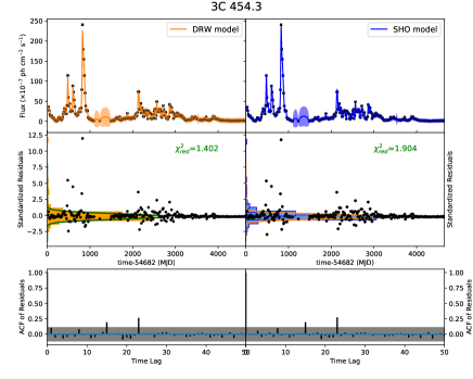
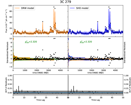
Figure 1: Fitting results of 3C 454.3 and 3C 279 for example. For each source, the left column presents results obtained from DRW model and we give the LAT LC (black points) and the modeled LC (orange line) in the top panel. In the middle panel, we show the standardized residuals (black points), the probability density of standardized residuals (orange histogram) as well as the best-fit normal distribution (green solid line). The reduced $\chi^{2}$ is labeled in the figure. The ACF of residuals with the 95$\%$ confidence limits of the white noise (the gray region) are shown in the bottom panel. The results obtained by the SHO model are given in the right column. The symbols and lines are the same as the left column but with different colors.

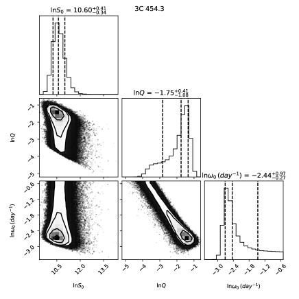
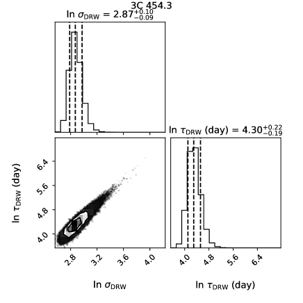
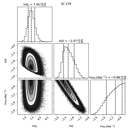
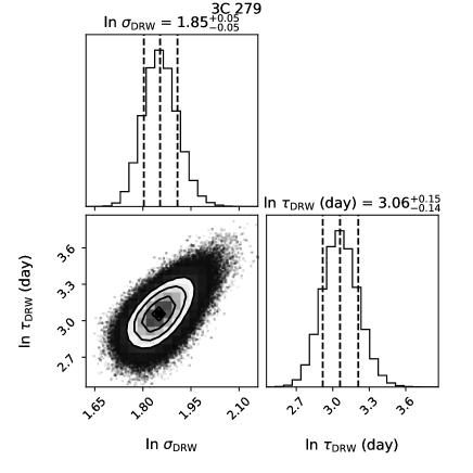
Figure 2: Posterior probability densities of model parameters for SHO (left) and DRW (right). The top panels are for 3C 454.3, and the bottom panels are for 3C 279. The vertical dotted lines mark the median value and 68$\%$ confidence intervals of the parameters distribution.

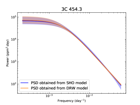
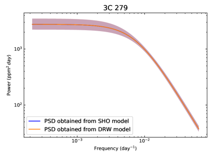
Figure 3: PSDs of the $\gamma$-ray LCs of 3C 454.3 (left) and 3C 279 (right) constructed from the modeling results with SHO (blue) and DRW (orange). The corresponding color region denotes $1\sigma$ confidence interval.

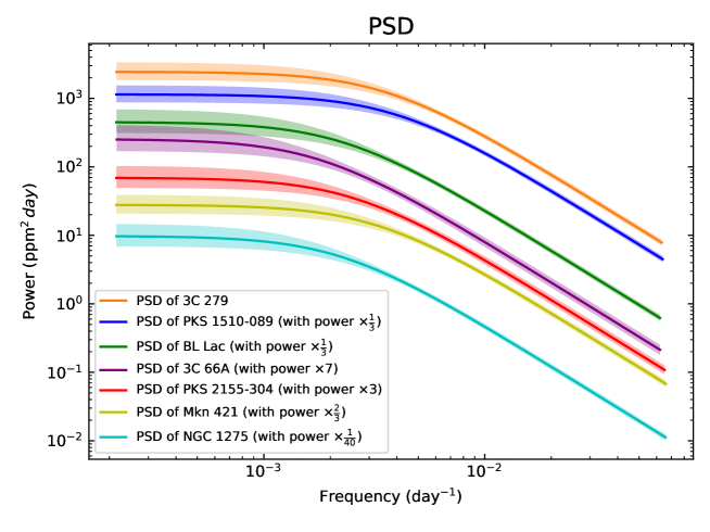
Figure 4: DRW PSDs for different types of AGNs.

5 Variability Characteristic Timescales in Relativistic Jets

Characteristic timescale is an important parameter in source variability. Our results show that DRW model can describe the $\gamma$-ray variability of 23 targets successfully, and the higher-order model SHO is unnecessary. From the fittings with the DRW model, we can obtain the characteristic timescales for the 23 sources. The characteristic (damping) timescales with errors in $1\sigma$ are given in Table 3. One can see that the timescales are between 20 days and 250 days. Note that the measurement of the damping timescale can be biased by the insufficient length of the LC (Kozłowski, 2017; Suberlak et al., 2021). Moreover, Burke et al. (2021) found that the measurement of damping timescale is reliable when it is larger than the typical cadence of LC. We use the following criteria to select the reliable measurements of the damping timescale: (1) The length of the LC should be ten times of the timescale at least; (2) The derived timescale should be larger than the mean cadence of the LC. It is found that all the $\gamma$-ray characteristic timescales for the 23 sources are reliable.

The LCs are fitted in the observed frame, and the values of the damping timescales in Table 3 are in the observed frame. In order to get the timescale in the rest frame ($\tau^{\rm rest}_{\rm damping}$), the timescale should be corrected by cosmological time dilation and and Doppler beaming effect,

$$\tau^{\rm rest}_{\rm damping}=\frac{\tau_{\rm DRW}\ \delta_{\rm D}}{1+z}\;,$$ (7)

where $\delta_{\rm D}$ is the Doppler factor. The Doppler factor for the $\gamma$-ray emission region in AGN jet is difficult to measure. It is estimated by different methods based on, for example, modeling the broadband spectral energy distributions (Chen, 2018; Pei et al., 2020), opacity of the $\gamma$-rays, and the brightness temperature of radio flare (Liodakis et al., 2017). In Table 4, we list the average values of $\delta_{\rm D}$ for different types of AGNs estimated by recent three papers (Liodakis et al., 2017; Chen, 2018; Pei et al., 2020). One can see that the uncertainties on the Doppler factor are very large. We use the average results of the three papers to correct the timescale. The average $\delta_{\rm D}$ for blazars is 10. It is found that $\tau^{\rm rest}_{\rm damping}$ is between 100 days and 1500 days, and the average $\tau^{\rm rest}_{\rm damping}$ is $\approx 510\$days.

The characteristic timescale in the optical variability of AGN accretion disk has been extensively studied (e.g., Collier & Peterson, 2001; Kelly et al., 2009; MacLeod et al., 2010; Simm et al., 2016; Suberlak et al., 2021). Recently, Burke et al. (2021) reported a correlation between the optical characteristic timescale and the black hole mass. We also show our results in the plot of $\tau^{\rm rest}_{\rm damping}-M_{\rm BH}$ (Figure 5), together with the results in Burke et al. (2021). It can be seen that the $\gamma$-ray variability timescales of AGNs occupy the same space with the optical variability timescales. Namely, in the same range of the black hole mass, the $\gamma$-ray variability timescales are consistent with the optical variability timescales within the errors. There is no correlation between the $\gamma$-ray variability timescale of AGN and the black hole mass. This is probably due to the small dynamic range in the black hole mass in the sample of $\sim 10^{8}-10^{9}M_{\rm\odot}$ (with the exception of NGC 1275) making any correlation difficult to be identified. We have searched the $\gamma$-ray AGNs with smaller black hole mass. However, they are not bright enough to perform the variability analysis. In Appendix A, we use the $\gamma$-ray flares from Crab Nebula to extend the mass of the central engine to much smaller range.

The $\gamma$-ray $\tau^{\rm rest}_{\rm damping}$ values slightly and systematically lie above the optical relation of Burke et al. (2021). In addition, we fit our $\gamma$-ray results and the optical results together, resulting in the best-fit relation,

$$\tau^{\rm rest}_{\rm damping}=154.22^{+14.76}_{-15.75}(\frac{M_{\rm{BH}}}{10^{8}M_{\rm{\odot}}})^{0.43^{+0.04}_{-0.04}}\;,$$ (8)

with an intrinsic scatter of $0.23\pm 0.03$ dex and Pearson correlation coefficient $r=0.80$. It is similar to the optical result.

We get the Eddington ratio (the ratio between accretion disk luminosity and the Eddington luminosity) for 15 out of 23 AGNs from Xiong et al. (2015), which are listed in Table 1. Except for Mrk 421, BL Lac and OJ 287, the rest of 12 sources have Eddington ratio between 0.01 and 1. From Figure 6, one can see that the 12 sources have similar Eddington ratio with the normal quasars in Burke et al. (2021), and the characteristic timescale is independent on the Eddington ratio.

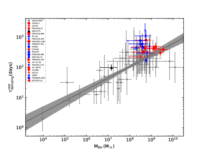
Figure 5: Variability damping timescale (in the rest frame) as a function of black hole mass. The gray data, lines and area represent optical results taken from Burke et al. (2021). The data in color are our results from the $\gamma$-ray LCs of AGNs. Data points in red, blue and black represent FSRQ, BLL and RDG, respectively.

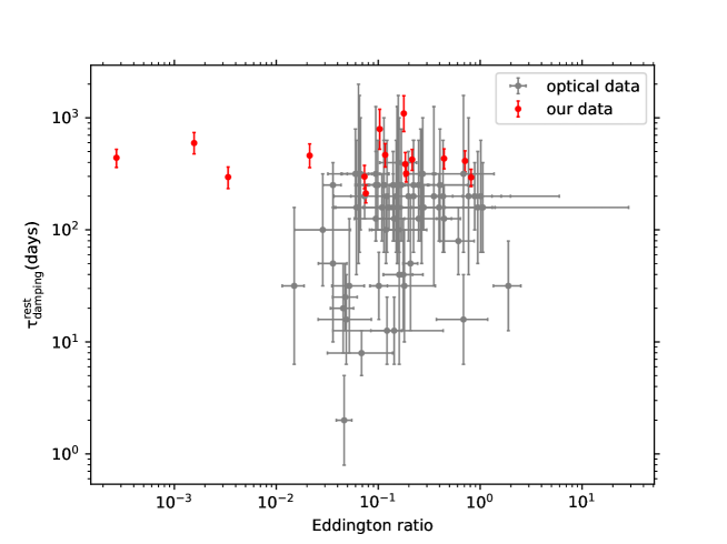
Figure 6: Plot of the rest-frame timescale versus the Eddington ratio. The gray data points with error bars are optical results taken from Burke et al. (2021). The data points in red denote the $\gamma$-ray results of blazars in our samples.

Table 4: Doppler factor for AGNs

FSRQ	BL Lac	RDG	Ref.
11	14	$\cdots$	1
15$\pm 9$	9$\pm 8$	1.4$\pm 0.8$	2
7$\pm 4$	4$\pm 3$	$\cdots$	3

Note. — Doppler factors with the errors for different types of AGNs taken from the references: (1) Chen (2018), (2) Liodakis et al. (2017), and (3) Pei et al. (2020).

6 Discussion

The stochastic process models are increasingly used to model $\gamma$-ray variability of blazars, providing an effective tool to study the statistical properties of the variability. We model the $\gamma$-ray variability of 23 bright LAT AGNs with the DRW and SHO models by performing the celerite package. It is found that the DRW model with two parameters can fit the $\gamma$-ray variability of 23 AGNs successfully, and the fits with the SHO model with three parameters for the 23 sources are not improved. The SHO is constrained in the over-damped mode ($Q<0.5$), and the strong degeneracy between $\omega_{0}$ and $Q$ leads to poor constraints on the two parameters. The PSDs of the 23 sources are typical DRW form with $f_{\rm b}$ between $0.001\ \rm day^{-1}$ and $0.01\ \rm day^{-1}$.

The brightest flares ($\gtrsim 10^{-5}\rm\ ph\ cm^{-2}\ s^{-1}$) in 3C 279 and 3C 454.3 are poorly fitted by both DRW and SHO models. Indeed, the extreme $\gamma$-ray flares in 3C 279 seem special (e.g., Shukla & Mannheim, 2020). The $\gamma$-ray photon index in the extreme flare on Dec 16 2012 is 1.7 (Hayashida et al., 2015), significantly smaller than the typical $\gamma$-ray photon index of 2.4 for FSRQ (Abdollahi et al., 2020). Minute-scale GeV $\gamma$-ray variability from 3C 279 was observed in an extreme flare on June 15 2016 (Ackermann et al., 2016). Nalewajko (2013) studied the individual $\gamma$-ray flares of 3C 454.3 with the flux above $0.71\times 10^{-5}\rm\ ph\ cm^{-2}\ s^{-1}$, and found that the $\gamma$-ray flares of 3C 454.3 have more complex light curves than other blazars. The extreme flares may have a different physical mechanism than the underlying long-term stochastic variability.

These brightest flares are expected to have impact on the slope of PSD at high frequencies (Ryan et al., 2019). We have examined that the brightest flares in 3C 279 and 3C 454.3 cannot affect the modeling results for the long-term variabilities. A further and careful study on the brightest flares is worthy of performing by using an adaptive binning algorithm.

The theoretical PSD expected by the one-zone leptonic emission model has been investigated (Finke & Becker, 2014, 2015; Chen et al., 2016). Thiersen et al. (2022) simulated multi-wavelength variability of blazars from a purely numerical approach by using a time-dependent one-zone leptonic emission model. They showed that a power-law PSD for the emission variability is produced by introducing stochastic variations for model parameters in the emission region, and the PSD is similar to the underlying power law of the model parameter variation. No spectral break is found in their produced PSDs. The results of Thiersen et al. (2022) indicate that in the frame of one-zone emission model, the physical processes associated with electron cooling, light crossing, and electron escape would not produce a break in the PSD. The broken frequencies we obtained are between $10^{-8}\$Hz and $10^{-7}\$Hz. The corresponding intrinsic timescale is several hundred days at least, which cannot be the timescale corresponding to electron cooling or acceleration process.

The $\gamma$-ray timescales of AGNs we obtained are very close to the optical timescales obtained from modeling AGN accretion disk emissions in Burke et al. (2021). Burke et al. (2021) speculated that the optical timescales could be associated with the thermal timescales expected in the AGN standard accretion disk theory, and the optical variability may be driven by the thermal instability of the accretion disk. The similarity between the $\gamma$-ray and optical characteristic timescales could imply a connection between jet and accretion disk. The thermal instability may also causes the $\gamma$-ray variability in the jet. However, the detailed mechanism that connects the accretion disk and the jet is unclear. The $\gamma$-ray timescales are slightly larger than the optical timescales of normal quasars. This may be due to that the distance from the $\gamma$-ray emission region to accretion disk extends the intrinsic timescale from accretion disk.

Ruan et al. (2012) modeled the nonthermal optical variabilities of 51 $\gamma$-ray blazars, and found that blazar optical $\tau^{\rm rest}_{\rm damping}$ peaks at $\sim$1000 days (assuming a typical Doppler factor of 10), which is systematically larger than the $\gamma$-ray $\tau^{\rm rest}_{\rm damping}$ in this work. The discrepancy between blazar $\gamma$-ray and optical $\tau^{\rm rest}_{\rm damping}$ may imply that the $\gamma$-ray and optical emissions are produced in different regions. The $\gamma$-ray emission region is closer to the accretion disk than the optical emission region. Ruan et al. (2012) found that blazar nonthermal optical characteristic timescales are $\sim$4 times smaller than normal quasars. They considered that the discrepancy between the optical characteristic timescales for blazars and normal quasars could be caused by the Doppler effect, if the jet variability and accretion disk variability have the same origin. Combining with our $\gamma$-ray results, we suppose that the discrepancy between the characteristic timescales for blazars and normal quasars is not only caused by the Doppler effect, but also related to the location of the jet emission region (the distance from the accretion disk). The jet long-term variability may be the convolution of the accretion disk variability with a transfer function which is related to Doppler factor and the distance from the jet emission region to the accretion disk at least.

7 Summary

We have applied a stochastic process method to the $\sim$12.7 yr Fermi-LAT LCs of 23 jetted AGNs in order to investigate the $\gamma$-ray variability properties. The SHO and DRW models are both used to model the long-term LCs. Our main results are as follows.

$(i)$ The long-term variability of 23 sources in our sample can be described well by both SHO and DRW models. However, the modelings with the SHO are not improved, and the parameters $\omega_{0}$ and $Q$ are poorly constrained. This suggests that the DRW model is preferred over the SHO model for the $\gamma$-ray long-term variability of AGNs. The PSDs for the 23 sources are the typical DRW PSD form.

$(ii)$ The intrinsic characteristic timescale of AGNs extracted from modeling the $\gamma$-ray variability is between 100 days to 1500 days. Such a long timescale cannot be produced in a one-zone leptonic emission model within the typical parameter space. In the plot of $\tau^{\rm rest}_{\rm damping}-M_{\rm BH}$, the $\gamma$-ray timescales obtained from jet emissions occupy almost the same space with the optical timescales obtained from the accretion disk emissions. Both the $\gamma$-ray and optical timescales are consistent with the thermal timescale expected by the AGN standard accretion disk. It may indicate a connection between the jet and the accretion disk.

In conclusion, our results suggest that the origin of the $\gamma$-ray variability could be related to the thermal instability in the accretion disk, however the detailed process that drives the variability is unclear.

Appendix A Crab Nebula $\gamma$-ray flare

GeV $\gamma$-ray flares from the Crab Nebula were observed by AGILE (Tavani et al., 2011) and Fermi-LAT (Abdo et al., 2011). The central pulsar, PSR B0531+21, has a mass of 1.4 solar mass. To extend the $\gamma$-ray $\tau^{\rm rest}_{\rm damping}$-mass relation to much smaller mass, we consider the $\gamma$-ray flares from the Crab Nebula. Huang et al. (2021) identified 17 flares in the $\gamma$-ray emission from Crab Nebula. The flare during MJD 55654.65-55678.65 has good sample and the flux uncertainties are relatively small. We use the DRW model to model 4-hr binning LC during MJD 55654.65-55678.65. The fitting results, PSD and posterior probability densities of parameters are shown in Figure 7 and Figure 8. We obtain the characteristic timescale $1.8^{+1.2}_{-0.8}$ days. This timescale is less than 1/10 of the length of the LC and larger than the mean cadence (0.36 days), which is reliable. We use the result to extend the $\gamma$-ray $\tau^{\rm rest}_{\rm damping}$-mass relation (Figure 9). There is a correlation (Pearson correlation coefficient $r=0.90$) between the $\gamma$-ray characteristic timescale and mass when adding the result of Crab Nebula, i.e.,

$$\tau^{\rm rest}_{\rm damping}=257.52^{+28.49}_{-33.21}(\frac{M_{\rm{BH}}}{10^{8}M_{\rm{\odot}}})^{0.26^{+0.04}_{-0.04}}\;,$$ (A1)

with an intrinsic scatter of $0.21\pm 0.05$ dex.

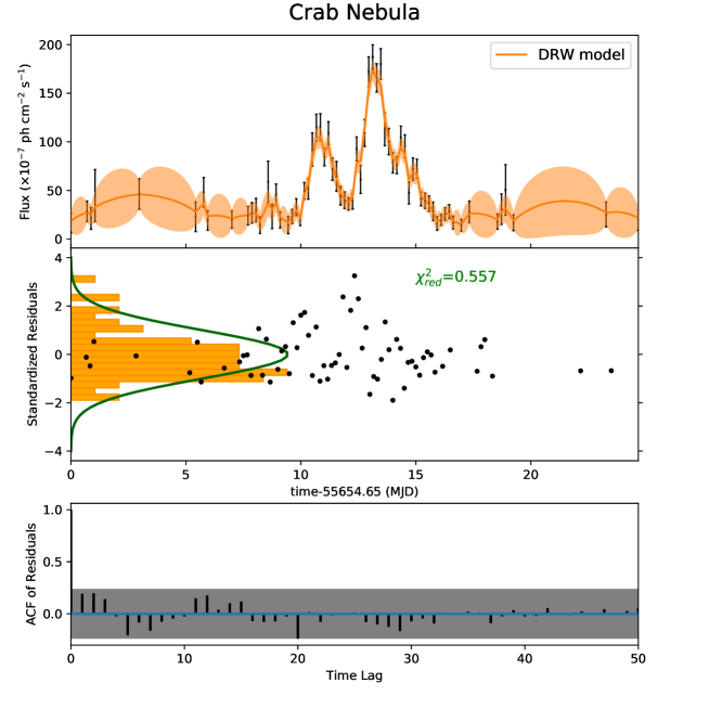
Figure 7: DRW modeling results of $\gamma$-ray flare (MJD 55654.65-55678.65) from the Crab Nebula. The symbols and lines are the same as those in Figure 1.

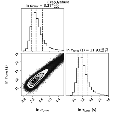
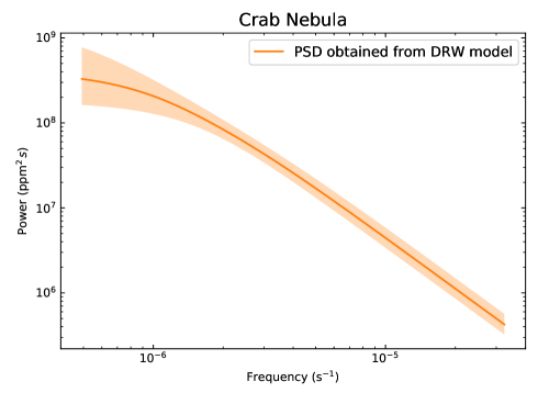
Figure 8: Left panel: posterior probability densities of DRW parameters for the Crab Nebula. The symbols and lines are the same as those in Figure 2. Right panel: DRW PSD of the $\gamma$-ray LC of the Crab Nebula. The corresponding color region denotes 1$\sigma$ confidence interval.

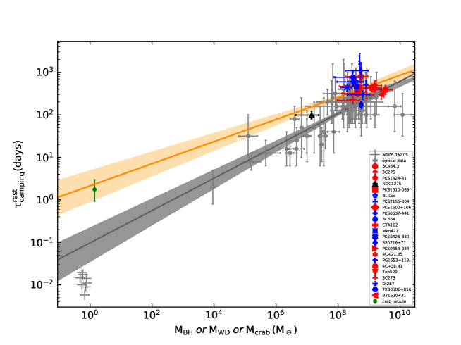
Figure 9: Variability damping timescale (in the rest frame) as a function of the mass of the central engine. The gray data, lines, area as well as the crosses represent optical results taken from Burke et al. (2021). The data in color are our results from the $\gamma$-ray LCs of AGNs and the Crab Nebula. The orange line and shaded band are the best-fit relation and 1$\sigma$ uncertainty for 23 AGNs and the Crab Nebula.

References

- Abdo et al. (2009) Abdo, A. A., Ackermann, M., Ajello, M., et al. 2009, ApJS, 183, 46, doi: 10.1088/0067-0049/183/1/46
- Abdo et al. (2010) —. 2010, ApJ, 722, 520, doi: 10.1088/0004-637X/722/1/520
- Abdo et al. (2011) —. 2011, Science, 331, 739, doi: 10.1126/science.1199705
- Abdollahi et al. (2020) Abdollahi, S., Acero, F., Ackermann, M., et al. 2020, ApJS, 247, 33, doi: 10.3847/1538-4365/ab6bcb
- Ackermann et al. (2015) Ackermann, M., Ajello, M., Albert, A., et al. 2015, ApJ, 813, L41, doi: 10.1088/2041-8205/813/2/L41
- Ackermann et al. (2016) Ackermann, M., Anantua, R., Asano, K., et al. 2016, ApJ, 824, L20, doi: 10.3847/2041-8205/824/2/L20
- Ait Benkhali et al. (2019) Ait Benkhali, F., Chakraborty, N., & Rieger, F. M. 2019, A&A, 623, A2, doi: 10.1051/0004-6361/201732334
- Ait Benkhali et al. (2020) Ait Benkhali, F., Hofmann, W., Rieger, F. M., & Chakraborty, N. 2020, A&A, 634, A120, doi: 10.1051/0004-6361/201935117
- Ajello et al. (2020) Ajello, M., Angioni, R., Axelsson, M., et al. 2020, ApJ, 892, 105, doi: 10.3847/1538-4357/ab791e
- Astropy Collaboration et al. (2013) Astropy Collaboration, Robitaille, T. P., Tollerud, E. J., et al. 2013, A&A, 558, A33, doi: 10.1051/0004-6361/201322068
- Astropy Collaboration et al. (2018) Astropy Collaboration, Price-Whelan, A. M., Sipőcz, B. M., et al. 2018, AJ, 156, 123, doi: 10.3847/1538-3881/aabc4f
- Bhatta & Dhital (2020) Bhatta, G., & Dhital, N. 2020, ApJ, 891, 120, doi: 10.3847/1538-4357/ab7455
- Burke et al. (2021) Burke, C. J., Shen, Y., Blaes, O., et al. 2021, Science, 373, 789, doi: 10.1126/science.abg9933
- Burnham & Anderson (2004) Burnham, K. P., & Anderson, D. R. 2004, Sociological Methods & Research, 33, 261, doi: 10.1177/0049124104268644
- Chen (2018) Chen, L. 2018, ApJS, 235, 39, doi: 10.3847/1538-4365/aab8fb
- Chen et al. (2016) Chen, X., Pohl, M., Böttcher, M., & Gao, S. 2016, MNRAS, 458, 3260, doi: 10.1093/mnras/stw528
- Collier & Peterson (2001) Collier, S., & Peterson, B. M. 2001, ApJ, 555, 775, doi: 10.1086/321517
- Covino et al. (2020) Covino, S., Landoni, M., Sandrinelli, A., & Treves, A. 2020, ApJ, 895, 122, doi: 10.3847/1538-4357/ab8bd4
- Covino et al. (2019) Covino, S., Sandrinelli, A., & Treves, A. 2019, MNRAS, 482, 1270, doi: 10.1093/mnras/sty2720
- Fan & Cao (2004) Fan, Z.-H., & Cao, X. 2004, ApJ, 602, 103, doi: 10.1086/380902
- Ferrarese et al. (2001) Ferrarese, L., Pogge, R. W., Peterson, B. M., et al. 2001, ApJ, 555, L79, doi: 10.1086/322528
- Finke & Becker (2014) Finke, J. D., & Becker, P. A. 2014, ApJ, 791, 21, doi: 10.1088/0004-637X/791/1/21
- Finke & Becker (2015) —. 2015, ApJ, 809, 85, doi: 10.1088/0004-637X/809/1/85
- Foreman-Mackey et al. (2017) Foreman-Mackey, D., Agol, E., Ambikasaran, S., & Angus, R. 2017, AJ, 154, 220, doi: 10.3847/1538-3881/aa9332
- Foreman-Mackey et al. (2013) Foreman-Mackey, D., Hogg, D. W., Lang, D., & Goodman, J. 2013, PASP, 125, 306, doi: 10.1086/670067
- Gebhardt et al. (2000) Gebhardt, K., Kormendy, J., Ho, L. C., et al. 2000, ApJ, 543, L5, doi: 10.1086/318174
- Ghisellini et al. (2010) Ghisellini, G., Tavecchio, F., Foschini, L., et al. 2010, MNRAS, 402, 497, doi: 10.1111/j.1365-2966.2009.15898.x
- Goyal et al. (2018) Goyal, A., Stawarz, Ł., Zola, S., et al. 2018, ApJ, 863, 175, doi: 10.3847/1538-4357/aad2de
- Gupta et al. (2012) Gupta, S. P., Pandey, U. S., Singh, K., et al. 2012, New A, 17, 8, doi: 10.1016/j.newast.2011.05.005
- H. E. S. S. Collaboration et al. (2017) H. E. S. S. Collaboration, Abdalla, H., Abramowski, A., et al. 2017, A&A, 598, A39, doi: 10.1051/0004-6361/201629419
- Harris et al. (2020) Harris, C. R., Millman, K. J., van der Walt, S. J., et al. 2020, Nature, 585, 357–362, doi: 10.1038/s41586-020-2649-2
- Hayashida et al. (2015) Hayashida, M., Nalewajko, K., Madejski, G. M., et al. 2015, ApJ, 807, 79, doi: 10.1088/0004-637X/807/1/79
- Huang et al. (2021) Huang, X., Yuan, Q., & Fan, Y.-Z. 2021, ApJ, 908, 65, doi: 10.3847/1538-4357/abd2b7
- Hunter (2007) Hunter, J. D. 2007, Computing in Science and Engineering, 9, 90, doi: 10.1109/MCSE.2007.55
- Kapanadze et al. (2020) Kapanadze, B., Gurchumelia, A., Dorner, D., et al. 2020, ApJS, 247, 27, doi: 10.3847/1538-4365/ab6322
- Kasliwal et al. (2017) Kasliwal, V. P., Vogeley, M. S., & Richards, G. T. 2017, MNRAS, 470, 3027, doi: 10.1093/mnras/stx1420
- Kaur et al. (2018) Kaur, N., Baliyan, K. S., Chandra, S., Sameer, & Ganesh, S. 2018, AJ, 156, 36, doi: 10.3847/1538-3881/aac5e4
- Kaur et al. (2017) Kaur, N., Sameer, Baliyan, K. S., & Ganesh, S. 2017, MNRAS, 469, 2305, doi: 10.1093/mnras/stx965
- Kelly et al. (2009) Kelly, B. C., Bechtold, J., & Siemiginowska, A. 2009, ApJ, 698, 895, doi: 10.1088/0004-637X/698/1/895
- Kelly et al. (2014) Kelly, B. C., Becker, A. C., Sobolewska, M., Siemiginowska, A., & Uttley, P. 2014, ApJ, 788, 33, doi: 10.1088/0004-637X/788/1/33
- Kozłowski (2017) Kozłowski, S. 2017, A&A, 597, A128, doi: 10.1051/0004-6361/201629890
- Li & Wang (2018) Li, Y.-R., & Wang, J.-M. 2018, MNRAS, 476, L55, doi: 10.1093/mnrasl/sly028
- Liodakis et al. (2017) Liodakis, I., Marchili, N., Angelakis, E., et al. 2017, MNRAS, 466, 4625, doi: 10.1093/mnras/stx002
- Liu et al. (2006) Liu, Y., Jiang, D. R., & Gu, M. F. 2006, ApJ, 637, 669, doi: 10.1086/498639
- MacLeod et al. (2010) MacLeod, C. L., Ivezić, Ž., Kochanek, C. S., et al. 2010, ApJ, 721, 1014, doi: 10.1088/0004-637X/721/2/1014
- MAGIC Collaboration et al. (2018) MAGIC Collaboration, Ansoldi, S., Antonelli, L. A., et al. 2018, A&A, 617, A91, doi: 10.1051/0004-6361/201832895
- Mattox et al. (1996) Mattox, J. R., Bertsch, D. L., Chiang, J., et al. 1996, ApJ, 461, 396, doi: 10.1086/177068
- McLure & Dunlop (2001) McLure, R. J., & Dunlop, J. S. 2001, MNRAS, 327, 199, doi: 10.1046/j.1365-8711.2001.04709.x
- Meyer et al. (2019) Meyer, M., Scargle, J. D., & Blandford, R. D. 2019, ApJ, 877, 39, doi: 10.3847/1538-4357/ab1651
- Moreno et al. (2019) Moreno, J., Vogeley, M. S., Richards, G. T., & Yu, W. 2019, PASP, 131, 063001, doi: 10.1088/1538-3873/ab1597
- Nakagawa & Mori (2013) Nakagawa, K., & Mori, M. 2013, ApJ, 773, 177, doi: 10.1088/0004-637X/773/2/177
- Nalewajko (2013) Nalewajko, K. 2013, MNRAS, 430, 1324, doi: 10.1093/mnras/sts711
- Padovani et al. (2019) Padovani, P., Oikonomou, F., Petropoulou, M., Giommi, P., & Resconi, E. 2019, MNRAS, 484, L104, doi: 10.1093/mnrasl/slz011
- Paliya et al. (2017) Paliya, V. S., Marcotulli, L., Ajello, M., et al. 2017, ApJ, 851, 33, doi: 10.3847/1538-4357/aa98e1
- Peñil et al. (2020) Peñil, P., Domínguez, A., Buson, S., et al. 2020, ApJ, 896, 134, doi: 10.3847/1538-4357/ab910d
- Pei et al. (2020) Pei, Z., Fan, J., Yang, J., & Bastieri, D. 2020, PASA, 37, e043, doi: 10.1017/pasa.2020.30
- Rakshit & Stalin (2017) Rakshit, S., & Stalin, C. S. 2017, ApJ, 842, 96, doi: 10.3847/1538-4357/aa72f4
- Rieger (2019) Rieger, F. 2019, Galaxies, 7, 28, doi: 10.3390/galaxies7010028
- Ruan et al. (2012) Ruan, J. J., Anderson, S. F., MacLeod, C. L., et al. 2012, ApJ, 760, 51, doi: 10.1088/0004-637X/760/1/51
- Ryan et al. (2019) Ryan, J. L., Siemiginowska, A., Sobolewska, M. A., & Grindlay, J. 2019, ApJ, 885, 12, doi: 10.3847/1538-4357/ab426a
- Sandrinelli et al. (2016) Sandrinelli, A., Covino, S., Dotti, M., & Treves, A. 2016, AJ, 151, 54, doi: 10.3847/0004-6256/151/3/54
- Sani et al. (2018) Sani, E., Ricci, F., La Franca, F., et al. 2018, Frontiers in Astronomy and Space Sciences, 5, 2, doi: 10.3389/fspas.2018.00002
- Sbarrato et al. (2012) Sbarrato, T., Ghisellini, G., Maraschi, L., & Colpi, M. 2012, MNRAS, 421, 1764, doi: 10.1111/j.1365-2966.2012.20442.x
- Shah et al. (2018) Shah, Z., Mankuzhiyil, N., Sinha, A., et al. 2018, Research in Astronomy and Astrophysics, 18, 141, doi: 10.1088/1674-4527/18/11/141
- Shaw et al. (2012) Shaw, M. S., Romani, R. W., Cotter, G., et al. 2012, ApJ, 748, 49, doi: 10.1088/0004-637X/748/1/49
- Shukla & Mannheim (2020) Shukla, A., & Mannheim, K. 2020, Nature Communications, 11, 4176, doi: 10.1038/s41467-020-17912-z
- Simm et al. (2016) Simm, T., Salvato, M., Saglia, R., et al. 2016, A&A, 585, A129, doi: 10.1051/0004-6361/201527353
- Sobolewska et al. (2014) Sobolewska, M. A., Siemiginowska, A., Kelly, B. C., & Nalewajko, K. 2014, ApJ, 786, 143, doi: 10.1088/0004-637X/786/2/143
- Suberlak et al. (2021) Suberlak, K. L., Ivezić, Ž., & MacLeod, C. 2021, ApJ, 907, 96, doi: 10.3847/1538-4357/abc698
- Tarnopolski et al. (2020) Tarnopolski, M., Żywucka, N., Marchenko, V., & Pascual-Granado, J. 2020, ApJS, 250, 1, doi: 10.3847/1538-4365/aba2c7
- Tavani et al. (2011) Tavani, M., Bulgarelli, A., Vittorini, V., et al. 2011, Science, 331, 736, doi: 10.1126/science.1200083
- Thiersen et al. (2022) Thiersen, H., Zacharias, M., & Böttcher, M. 2022, ApJ, 925, 177, doi: 10.3847/1538-4357/ac4013
- Tremaine et al. (2002) Tremaine, S., Gebhardt, K., Bender, R., et al. 2002, ApJ, 574, 740, doi: 10.1086/341002
- Virtanen et al. (2020) Virtanen, P., Gommers, R., Oliphant, T. E., et al. 2020, Nature Methods, 17, 261, doi: 10.1038/s41592-019-0686-2
- Wang et al. (2004) Wang, J.-M., Luo, B., & Ho, L. C. 2004, ApJ, 615, L9, doi: 10.1086/426060
- Xiong et al. (2015) Xiong, D., Zhang, X., Bai, J., & Zhang, H. 2015, MNRAS, 450, 3568, doi: 10.1093/mnras/stv812
- Yan et al. (2018) Yan, D., Yang, S., Zhang, P., et al. 2018, ApJ, 864, 164, doi: 10.3847/1538-4357/aadd01
- Yang et al. (2021) Yang, S., Yan, D., Zhang, P., Dai, B., & Zhang, L. 2021, ApJ, 907, 105, doi: 10.3847/1538-4357/abcbff
- Zhang et al. (2021) Zhang, H., Yan, D., Zhang, P., Yang, S., & Zhang, L. 2021, ApJ, 919, 58, doi: 10.3847/1538-4357/ac0cf0
- Zhang et al. (2018) Zhang, H., Yang, Q., & Wu, X.-B. 2018, ApJ, 853, 116, doi: 10.3847/1538-4357/aaa3e5
- Zhang et al. (2020) Zhang, P.-f., Yan, D.-h., Zhou, J.-n., Wang, J.-c., & Zhang, L. 2020, ApJ, 891, 163, doi: 10.3847/1538-4357/ab71fe
- Zhou et al. (2018) Zhou, J., Wang, Z., Chen, L., et al. 2018, Nature Communications, 9, 4599, doi: 10.1038/s41467-018-07103-2
- Zu et al. (2013) Zu, Y., Kochanek, C. S., Kozłowski, S., & Udalski, A. 2013, ApJ, 765, 106, doi: 10.1088/0004-637X/765/2/106