Convergence analysis of a Local Discontinuous Galerkin approximation for nonlinear systems with balanced Orlicz-structure

Abstract.

In this paper, we investigate a Local Discontinuous Galerkin (LDG) approximation for systems with balanced Orlicz-structure. We propose a new numerical flux, which yields optimal convergence rates for linear ansatz functions. In particular, our approach yields a unified treatment for problems with $(p,\delta)$-structure for arbitrary $p\in(1,\infty)$ and $\delta\geq 0$.

1. Introduction

We consider the numerical approximation of the nonlinear system

$$-\operatorname{div}\boldsymbol{\mathcal{A}}(\nabla{\bf u}) ={\bf g}-\operatorname{div}{\bf G}\qquad \text{in }\Omega\,,$$ (1.1)

$${\bf u} ={\bf u}_{D}\qquad \text{on }\Gamma_{D}\,,$$

$$\boldsymbol{\mathcal{A}}(\nabla{\bf u}){\bf n} ={\bf a}_{N} \text{on }\Gamma_{N}\,,$$

using a Local Discontinuous Galerkin (LDG) scheme. More precisely, for given data ${\bf g}$, ${\bf G}$, ${\bf u}_{D}$ and ${\bf a}_{N}$, we seek a vector field ${\bf u}=(u_{1},\ldots,u_{d})^{\top}:\Omega\to\mathbb{R}^{d}$ solving (1.1). Here, $\Omega\subseteq\mathbb{R}^{n}$, $n\geq 2$, is a polyhedral, bounded domain with Lipschitz continuous boundary $\partial\Omega$, which is disjointly divided into a Dirichlet part $\Gamma_{D}$, where we assume that ${{\lvert{\Gamma_{D}}\rvert}\!>\!0}$, and a Neumann part $\Gamma_{N}$, i.e., $\Gamma_{D}\cup\Gamma_{N}=\partial\Omega$ and $\Gamma_{D}\cap\Gamma_{N}=\emptyset$. By ${\bf n}:\partial\Omega\to\mathbb{S}^{n-1}$, we denote the unit normal vector field to $\partial\Omega$ pointing outward. We consider the case that $\boldsymbol{\mathcal{A}}\colon\mathbb{R}^{d\times n}\to\mathbb{R}^{d\times n}$ is a nonlinear operator having $\varphi$-structure for some balanced N-function $\varphi$ (cf. Section 2.2). The relevant example falling into this class is

$$\boldsymbol{\mathcal{A}}(\nabla{\bf u})=\frac{\varphi^{\prime}\big{(}{\lvert{\nabla{\bf u}}\rvert}\big{)}}{{\lvert{\nabla{\bf u}}\rvert}}\,\nabla{\bf u}\,.$$

Introducing the additional unknowns ${\bf L}:\Omega\to\mathbb{R}^{d\times n}$ and ${\bf A}:\Omega\to\mathbb{R}^{d\times n}$, the system (1.1) can be re-written as a ”first order” system, i.e.,

$$\begin{aligned} {\bf L}=\nabla{\bf u}\,,\quad{\bf A}&=\boldsymbol{\mathcal{A}}({\bf L})\,,\quad-\operatorname{div}{\bf A}={\bf g}-\operatorname{div}{\bf G}&\qquad&\text{in $\Omega$}\,,\\[-1.42262pt] {\bf u}&={\bf u}_{D}&\qquad&\text{on $\Gamma_{D}$}\,,\\[-1.42262pt] {\bf A}{\bf n}&={\bf a}_{N}&\qquad&\text{on $\Gamma_{N}$}\,.\end{aligned}$$ (1.2)

Discontinuous Galerkin (DG) methods for elliptic problems have been introduced in the late 90’s. They are by now well-understood and rigorously analyzed in the context of linear elliptic problems (cf. [2] for the Poisson problem). In contrast to this, only few papers treat $p$-Laplace type problems with DG methods (cf. [11, 10, 17, 12, 23, 25]), or non-conforming methods (cf. [5]). There exists even fewer numerical investigations of problems with Orlicz-structure. Steady problems with Orlicz-structure are treated, using finite element methods (FEM) in [18, 16, 9] and non-conforming methods in [5]. Unsteady problems are investigated in [20, 27]. To the best of the author’s knowledge, there are no studies of steady problems with Orlicz-structure using DG methods, except for [17, Remark 2.3], where it is mentioned that the results for the $p$-Laplace can be extended to balanced N-functions. Note that the convergence rates in [17] are sub-optimal (cf. Remark 5.24) since the continuous solution ${\bf u}$ of (1.1) satisfies the flux formulation of (1.1) with an additional term defined on interior and Dirichlet faces (cf. (5.1)). The main purpose of this paper is to overcome this drawback. Moreover, we state our results in the context of balanced N-functions to make clear that the usual distinction between the cases $p\geq 2$ and $p\leq 2$ for $p$-Laplace problems is not needed.

To this end, we introduce a new numerical flux (cf. (3.4)), which allows us to establish convergence of DG-solutions to a weak solution of the system (1.1) for general right-hand sides ${\bf g}-\operatorname{div}{\bf G}$ (cf. Theorem 4.27), and error estimates if ${\bf G}={\mathbf{0}}$ (cf. Theorem 5.10, Corollary 5.22). The convergence rates are optimal for linear ansatz functions. Further, our approach yields a unified treatment of problems with $(p,\delta)$-structure (cf. [17]), ${p\in(1,\infty)}$, ${\delta\geq 0}$ and recovers in the DG setting the results in [19, 18] (using FEM) and [5] (using special non-conforming methods). The presence of the shift in the new flux is analogous to the gradient shift in the natural distance. It takes into account the structure of the nonlinear problem (1.1) (cf. Proposition 2.17, Remark 2.30, Remark 5.24).

This paper is organized as follows: ​In Section 2, we introduce the employed notation, define the relevant function spaces, the basic assumptions on the nonlinear operator and its consequences, introduce discrete operators and discuss their properties. In Section 3, we define our numerical fluxes and derive the flux and the primal formulation of our problem. In Section 4, we prove the existence of DG solutions (cf. Proposition 4.19), the stability of the method, i.e., a priori estimates (cf. Proposition 4.21, Corollary 4.23), and the convergence of DG solutions (cf. Theorem 4.27). In Section 5, we derive error estimates for our problem (cf. Theorem 5.10, Corollary 5.22). These are the first convergence rates for an LDG method for systems with balanced Orlicz-structure. In Section 6, we confirm our theoretical findings via numerical experiments. For the convenience of the reader, we collect in the Appendix A known results in the DG Orlicz setting, needed in the paper, and prove some new results.

2. Preliminaries

2.1. Function spaces

We use $c,C\!>\!0$ to denote generic constants, that may change from line to line, but are not depending on the crucial quantities. Moreover, we write ${f\sim g}$ if and only if there exists constants $c,C>0$ such that $c\,f\leq g\leq C\,f$.

For $k\in\mathbb{N}$ and $p\in[1,\infty]$, we will employ the customary Lebesgue spaces $L^{p}(\Omega)$ and Sobolev spaces $W^{k,p}(\Omega)$, where $\Omega\subseteq\mathbb{R}^{n}$, $n\geq 2$, is a bounded, polyhedral domain ha-ving a Lipschitz continuous boundary $\partial\Omega$, which is disjointly divided into a Dirichlet part $\Gamma_{D}\subseteq\partial\Omega$, where we assume that ${\lvert{\Gamma_{D}}\rvert}>0$, and a Neumann part $\Gamma_{N}\subseteq\partial\Omega$, i.e., $\Gamma_{D}\cup\Gamma_{N}\!=\!\partial\Omega$ and $\Gamma_{D}\cap\Gamma_{N}\!=\!\emptyset$. We denote by $\smash{{\lVert{\,\cdot\,}\rVert}_{p}}$, the norm in $L^{p}(\Omega)$ and by $\smash{{\lVert{\,\cdot\,}\rVert}_{k,p}}$, the norm in $W^{k,p}(\Omega)$. The space $\smash{W^{1,p}_{\Gamma_{D}}(\Omega)}$ is defined as those functions from $W^{1,p}(\Omega)$ whose trace vanishes on $\Gamma_{D}$. We equip $\smash{W^{1,p}_{\Gamma_{D}}(\Omega)}$ with the gradient norm $\smash{{\lVert{\nabla\,\cdot\,}\rVert}_{p}}$.

For a normed vector space $X$, we denote its (topological) dual space by $X^{*}$. We do not distinguish between function spaces for scalar, vector- or tensor-valued functions. However, we will denote vector-valued functions by boldface letters and tensor-valued functions by capital boldface letters. For $d\in\mathbb{N}$, the standard scalar product between two vectors ${\bf u}=(u_{1},\dots,u_{d})^{\top},{\bf v}=(v_{1},\dots,v_{d})^{\top}\in\mathbb{R}^{d}$ is denoted by ${{\bf u}\cdot{\bf v}=\sum_{i=1}^{d}{u_{i}v_{i}}}$, and we use the notation $|{\bf u}|=\sqrt{{\bf u}\cdot{\bf u}}$ for all ${\bf u}\in\mathbb{R}^{d}$. For $d,n\in\mathbb{N}$, the Frobenius scalar product between two tensors ${{\bf P}\!=\!(P_{ij})_{i=1,\dots,d,j=1,\dots,n},\!{\bf Q}\!=\!(Q_{ij})_{i=1,\dots,d,j=1,\dots,n}\!\in\!\mathbb{R}^{d\times n}}$ is denoted by ${\bf P}:{\bf Q}\!=\!\sum_{i=1}^{d}{\sum_{j=1}^{n}{P_{ij}Q_{ij}}}$, and we write ${\lvert{{\bf P}}\rvert}\!=\!\sqrt{{\bf P}:{\bf P}}$ for all ${{\bf P}\!\in\!\mathbb{R}^{d\times n}}$. We denote by ${\lvert{M}\rvert}$, the $n$– or $(n-1)$–dimensional Lebesgue measure of a (Lebesgue) measurable set $M\subseteq\mathbb{R}^{n}$, $n\in\mathbb{N}$. The mean value of a locally integrable function $f$ over a measurable set $M\!\subseteq\!\Omega$ is denoted by ${\langle{f}\rangle_{M}\!\vcentcolon=\!\smash{\mathop{\mathchoice{{\vbox{\hbox{$\textstyle-$}}\kern-4.86108pt}}{{\vbox{\hbox{$\scriptstyle-$}}\kern-3.25pt}}{{\vbox{\hbox{$\scriptscriptstyle-$}}\kern-2.29166pt}}{{\vbox{\hbox{$\scriptscriptstyle-$}}\kern-1.875pt}}\!\int}_{M}f\,\textup{d}x}\!\vcentcolon=\!\smash{\frac{1}{|M|}\int_{M}f\,\textup{d}x}}$. Moreover, we use the notation ${({f},{g})}\vcentcolon=\int_{\Omega}fg\,\textup{d}x$, whenever the right-hand side is well-defined.

We will also use Orlicz and Sobolev–Orlicz spaces (cf. [26]). A real convex function $\psi:\mathbb{R}^{\geq 0}\to\mathbb{R}^{\geq 0}$ is said to be an N-function, if $\psi(0)=0$, $\psi(t)>0$ for all ${t>0}$, $\lim_{t\rightarrow 0}\psi(t)/t=0$, and $\lim_{t\rightarrow\infty}\psi(t)/t=\infty$. We call $\psi$ a regular N-function, if it, in addition, belongs to $C^{1}(\mathbb{R}^{\geq 0})\cap C^{2}(\mathbb{R}^{>0})$ and satisfies ${\psi^{\prime\prime}(t)>0}$ for all ${t>0}$. For a regular N-function, we have $\psi(0)=\psi^{\prime}(0)=0$, $\psi^{\prime}$ is increasing and $\lim_{t\to\infty}\psi^{\prime}(t)=\infty$. We define the (convex) conjugate N-function $\psi^{*}$ by ${\psi^{*}(t)\vcentcolon=\sup_{s\geq 0}(st-\psi(s))}$ for all ${t\!\geq\!0}$, which satisfies $(\psi^{*})^{\prime}\!=\!(\psi^{\prime})^{-1}\!\!$. A given N-function $\psi$ satisfies the $\Delta_{2}$-condition (in short, $\varphi\in\Delta_{2}$), if there exists $K>2$ such that for all $t\geq 0$, it holds ${\psi(2\,t)\leq K\,\psi(t)}$. We denote the smallest such constant by $\Delta_{2}(\psi)>0$. If one assumes that both $\psi$ and $\psi^{*}$ satisfy the $\Delta_{2}$-condition, there holds

$$\smash{\psi^{*}\circ\psi^{\prime}\sim\psi\,.}$$ (2.1)

We need the following refined version of the $\varepsilon$-Young inequality: for every ${\varepsilon\!>\!0}$, there is a $c_{\varepsilon}>0$, depending only on $\Delta_{2}(\psi),\Delta_{2}(\psi^{*})<\infty$, such that for all ${s,t\geq 0}$, it holds

$$\begin{split}t\,s&\leq\varepsilon\,\psi(t)+c_{\varepsilon}\,\psi^{*}(s)\,,\\ t\,\psi^{\prime}(s)+\psi^{\prime}(t)\,s&\leq\varepsilon\,\psi(t)+c_{\varepsilon}\,\psi(s)\,.\end{split}$$ (2.2)

We denote by $L^{\psi}(\Omega)$ and $W^{1,\psi}(\Omega)$, the classical Orlicz and Sobolev–Orlicz spaces, i.e., we have that $f\in L^{\psi}(\Omega)$ if the modular $\rho_{\psi}(f)=\rho_{\psi,\Omega}(f)\vcentcolon=\int_{\Omega}\psi({\lvert{f}\rvert})\,\textup{d}x$ is finite and ${f\in W^{1,\psi}(\Omega)}$ if $f,\nabla f\in L^{\psi}(\Omega)$. Equipped with the induced Luxembourg norm, i.e., $\smash{{\lVert{f}\rVert}_{\psi}}\vcentcolon=\smash{\inf{\{{\lambda>0\mid\int_{\Omega}\psi({\lvert{f}\rvert}/\lambda)\,\textup{d}x\leq 1}\}}}$, the space $L^{\psi}(\Omega)$ forms a Banach space. The same holds for the space $W^{1,\psi}(\Omega)$ if it is equipped with the norm $\smash{{\lVert{\,\cdot\,}\rVert}_{\psi}+{\lVert{\nabla\,\cdot\,}\rVert}_{\psi}}$. Note that the dual space $(L^{\psi}(\Omega))^{*}$ of $L^{\psi}(\Omega)$ can be identified with the space $L^{\psi^{*}}(\Omega)$. The space $\smash{W^{1,\psi}_{\Gamma_{D}}(\Omega)}$ is defined as those functions from $W^{1,\psi}(\Omega)$ whose trace vanishes on $\Gamma_{D}$. We equip $\smash{W^{1,\psi}_{\Gamma_{D}}(\Omega)}$ with the gradient norm $\smash{{\lVert{\nabla\,\cdot\,}\rVert}_{\psi}}$.

2.2. Basic properties of the nonlinear operator

In the whole paper, we always assume that the nonlinear operator $\boldsymbol{\mathcal{A}}:\mathbb{R}^{d\times n}\to\mathbb{R}^{d\times n}$ has $\varphi$-structure, which will be defined now. A detailed discussion and thorough proofs can be found in [14, 29, 8]. A regular N-function $\psi$ is called balanced, if there exist constants ${\gamma_{1}\in(0,1]}$ and ${\gamma_{2}\geq 1}$ such that for all $t>0$, there holds

$$\smash{\gamma_{1}\,\psi^{\prime}(t)\leq t\,\psi^{\prime\prime}(t)\leq\gamma_{2}\,\psi^{\prime}(t)}\,.$$ (2.3)

The constants $\gamma_{1}$ and $\gamma_{2}$ are called characteristics of the balanced N-function $\psi$, and will be denoted as $(\gamma_{1},\gamma_{2})$. The basic properties of balanced N-functions are collected in the following lemma (cf. [15] for related results of a slightly different approach).

Lemma 2.4.

Let $\psi$ be a balanced N-function with characteristics $(\gamma_{1},\gamma_{2})$. Then, the following statements apply:

• The conjugate N-function $\psi^{\ast}\!$ is a balanced N-function with characteristics $(\frac{1}{\gamma_{1}},\!\frac{1}{\gamma_{2}})$.

• The N-functions $\psi$ and $\psi^{\ast}$ satisfy the $\Delta_{2}$-condition, and the $\Delta_{2}$-constants of $\psi$ and $\psi^{*}$ possess an upper bound depending only on the characteristics of $\psi$.

• Uniformly with respect to $t>0$, we have that $\psi(t)\sim\psi^{\prime}(t)\,t\sim\psi^{\prime\prime}(t)\,t^{2}$, with constants of equivalence depending only on the characteristics of $\psi$.

Proof.

The assertion (i) is proved in [29, Lemma 6.4]. The assertion (ii) is proved in [7] (cf. [8, Lemma 2.10]). Assertion (iii) follows from (ii), since for N-functions satisfying the $\Delta_{2}$-condition, uniformly with respect to $t>0$, there holds

$$\smash{\psi^{\prime}(t)\,t\sim\psi(t)\,,}$$ (2.5)

and the fact that $\psi$ is balanced. ∎

Remark 2.6.

It is well-known that the N-function $\psi$ for which $\psi^{\prime}(t)=(\delta+t)^{p-2}t$ for all $t\geq 0$, $p\in(1,\infty)$, $\delta\geq 0$, is balanced (cf. [29, 18]). Other examples are given via $\psi^{\prime}(t)\!=\!(t^{\alpha}(\delta+t)^{1-\alpha})^{p-2}t$ for all $t\!\geq\!0$, or ${\psi^{\prime}(t)\!=\!(t\!+\!\delta)^{p-2}t(\ln(1\!+\!\delta+\!t))^{\alpha}}$ for all ${t\!\geq\!0}$, where ${\alpha\geq 1}$, $p\!\in\!(1,\infty)$, ${\delta\!\geq\!0}$.

Assumption 2.7 (Nonlinear operator).

We assume that the nonlinear operator ${\boldsymbol{\mathcal{A}}\colon\mathbb{R}^{d\times n}\to\mathbb{R}^{d\times n}}$ belongs to $C^{0}(\mathbb{R}^{d\times n},\mathbb{R}^{d\times n})\cap C^{1}(\mathbb{R}^{d\times n}\setminus\{{\mathbf{0}}\},\mathbb{R}^{d\times n})$ and satisfies $\boldsymbol{\mathcal{A}}(\mathbf{0})=\mathbf{0}$. Moreover, we assume that the operator $\boldsymbol{\mathcal{A}}$ has $\varphi$-structure, i.e., there exist a regular N-function $\varphi$ and constants $\gamma_{3}\in(0,1]$, $\gamma_{4}>1$ such that

$$\sum\nolimits_{j,l=1}^{n}\sum\nolimits_{i,k=1}^{d}\partial_{kl}\mathcal{A}_{ij}({\bf P})Q_{ij}Q_{kl} \geq\gamma_{3}\,\frac{\varphi^{\prime}(|{\bf P}|)}{|{\bf P}|}|{\bf Q}|^{2}\,,$$ (2.8a)

$$\big{|}\partial_{kl}\mathcal{A}_{ij}({{\bf P}})\big{|} \leq\gamma_{4}\,\frac{\varphi^{\prime}(|{\bf P}|)}{|{\bf P}|}\,,$$ (2.8b)

are satisfied for all ${\bf P},{\bf Q}\in\mathbb{R}^{d\times n}$ with ${\bf P}\neq{\mathbf{0}}$ and all $i,k=1,\ldots,d$, $j,l=1,\ldots,n$. The constants $\gamma_{3}$, $\gamma_{4}$, and $\Delta_{2}(\varphi)$ are called the characteristics of $\boldsymbol{\mathcal{A}}$ and will be denoted by $(\gamma_{3},\gamma_{4},\Delta_{2}(\varphi))$.

Closely related to the nonlinear operator $\boldsymbol{\mathcal{A}}\colon\mathbb{R}^{d\times n}\to\mathbb{R}^{d\times n}$ with $\varphi$-structure are the functions ${\bf F},{\bf F}^{*}\colon\mathbb{R}^{d\times n}\to\mathbb{R}^{d\times n}$, for every ${\bf P}\in\mathbb{R}^{d\times n}$ defined via

$$\begin{aligned} {\bf F}({\bf P})\vcentcolon=\sqrt{\frac{\varphi^{\prime}({\lvert{{\bf P}}\rvert})}{{\lvert{{\bf P}}\rvert}}}\,{\bf P}\,,\qquad{\bf F}^{*}({\bf P})\vcentcolon=\sqrt{\frac{(\varphi^{*})^{\prime}({\lvert{{\bf P}}\rvert})}{{\lvert{{\bf P}}\rvert}}}\,{\bf P}\,.\end{aligned}$$ (2.9)

Remark 2.10.

Note that ${\bf F}$ and ${\bf F}^{*}$ are derived from the potentials

$$\kappa(t)\vcentcolon=\int_{0}^{t}\sqrt{\varphi^{\prime}(s)\,s}\,\mathrm{d}s\quad\textrm{ and }\quad\kappa^{*}(t)\vcentcolon=\int_{0}^{t}\sqrt{(\varphi^{*})^{\prime}(s)\,s}\,\mathrm{d}s\quad\textup{ for all }t\geq 0\,,$$

respectively. One easily sees that these potentials are balanced N-functions.

Another important tool are the shifted N-functions (cf. [14, 29, 28]). For a given N-function $\psi$, we define the shifted N–functions ${\psi_{a}:\mathbb{R}^{\geq 0}\to\mathbb{R}^{\geq 0}}$, ${a\geq 0}$, via

$$\psi_{a}(t)\vcentcolon=\int_{0}^{t}\psi_{a}^{\prime}(s)\,\textup{d}s\qquad\text{with }\quad\psi^{\prime}_{a}(t)\vcentcolon=\psi^{\prime}(a+t)\frac{t}{a+t}\quad\textup{ for all }t\geq 0\,.$$ (2.11)

The following properties of shifted N-functions are proved in [14, 29].

Lemma 2.12.

Let the N-functions $\psi,\psi^{*}$ satisfy the $\Delta_{2}$-condition. Then, it holds:

• The family of shifted N-functions ${\psi_{a}:\mathbb{R}^{\geq 0}\to\mathbb{R}^{\geq 0}}$, ${a\geq 0}$, satisfy the $\Delta_{2}$-con-dition uniformly with respect to $a\geq 0$ with $\Delta_{2}(\psi_{a})$ depending only on $\Delta_{2}(\psi)$.

• The conjugate function satisfies $\smash{(\psi_{a})^{*}(t)\sim(\psi^{*})_{\psi^{\prime}(a)}(t)}$ uniformly with respect to ${t,a\geq 0}$ with constants depending only on $\Delta_{2}(\psi),\Delta_{2}(\psi^{*})$.

Lemma 2.13.

Let $\psi$ be an N–function satisfying the $\Delta_{2}$-condition. Then, there exists a constant $c>0$ such that for every ${{\bf P},{\bf Q}\in\mathbb{R}^{d\times n}}$ and $t\geq 0$, we have that

$$\smash{\psi_{{\lvert{{\bf P}}\rvert}}^{\prime}(t)\leq c\,\psi_{{\lvert{{\bf Q}}\rvert}}^{\prime}(t)+c\,\psi_{{\lvert{{\bf P}}\rvert}}^{\prime}({\lvert{{\bf P}-{\bf Q}}\rvert})\,.}$$ (2.14)

Moreover, $\psi_{\lvert{{\bf Q}}\rvert}^{\prime}({\lvert{{\bf P}-{\bf Q}}\rvert})\sim\psi_{\lvert{{\bf P}}\rvert}^{\prime}({\lvert{{\bf P}-{\bf Q}}\rvert})$ holds uniformly with respect to ${{\bf P},{\bf Q}\in\mathbb{R}^{d\times n}}$.

Lemma 2.15 (Change of shift).

Let $\psi$ be an N–function such that $\psi$ and $\psi^{*}$ satisfy the $\Delta_{2}$–condition. Then, for every $\delta\in(0,1)$, there exists $c_{\delta}>0$ such that for every ${\bf P},{\bf Q}\in\mathbb{R}^{d\times n}$ and $t\geq 0$, we have that

$$\begin{aligned} \psi_{{\lvert{{\bf P}}\rvert}}(t)&\leq c_{\delta}\,\psi_{{\lvert{{\bf Q}}\rvert}}(t)+\delta\,\psi_{{\lvert{{\bf P}}\rvert}}({\lvert{{\bf P}-{\bf Q}}\rvert})\,,\\ \big{(}\psi_{{\lvert{{\bf P}}\rvert}}\big{)}^{*}(t)&\leq c_{\delta}\,\big{(}\psi_{{\lvert{{\bf Q}}\rvert}}\big{)}^{*}(t)+\delta\,\psi_{{\lvert{{\bf P}}\rvert}}({\lvert{{\bf P}-{\bf Q}}\rvert})\,.\end{aligned}$$ (2.16)

Moreover, $\psi_{\lvert{{\bf Q}}\rvert}({\lvert{{\bf P}-{\bf Q}}\rvert})\sim\psi_{\lvert{{\bf P}}\rvert}({\lvert{{\bf P}-{\bf Q}}\rvert})$ holds uniformly with respect to ${{\bf P},{\bf Q}\in\mathbb{R}^{d\times n}}$.

The connection between $\boldsymbol{\mathcal{A}},{\bf F},{\bf F}^{*}\colon\mathbb{R}^{d\times n}\to\mathbb{R}^{d\times n}$ and $\varphi_{a},(\varphi^{*})_{a}:\mathbb{R}^{\geq 0}\to\mathbb{R}^{\geq 0}$, ${a\geq 0}$, is best explained by the following proposition (cf. [14, 29]).

Proposition 2.17.

Let $\boldsymbol{\mathcal{A}}$ satisfy Assumption 2.7 for a balanced N-function ${\varphi}$. Then, uniformly with respect to ${\bf P},{\bf Q}\in\mathbb{R}^{d\times n}$, we have that

$$\big{(}\boldsymbol{\mathcal{A}}({\bf P})-\boldsymbol{\mathcal{A}}({\bf Q})\big{)}:({\bf P}-{\bf Q}) \sim\smash{{\lvert{{\bf F}({\bf P})-{\bf F}({\bf Q})}\rvert}^{2}}\sim\varphi_{{\lvert{{\bf P}}\rvert}}({\lvert{{\bf P}-{\bf Q}}\rvert})\,,$$ (2.18)

$$\smash{{\lvert{{\bf F}^{*}({\bf P})-{\bf F}^{*}({\bf Q})}\rvert}^{2}} \sim\smash{\smash{\big{(}\varphi^{*}\big{)}}_{\smash{{\lvert{{\bf P}}\rvert}}}({\lvert{{\bf P}-{\bf Q}}\rvert})}\,,$$ (2.19)

$${\lvert{\boldsymbol{\mathcal{A}}({\bf P})-\boldsymbol{\mathcal{A}}({\bf Q})}\rvert} \sim\smash{\varphi^{\prime}_{{\lvert{{\bf P}}\rvert}}({\lvert{{\bf P}-{\bf Q}}\rvert})}\,.$$ (2.20)

Moreover, uniformly with respect to $$\smash{{\bf Q}\in\mathbb{R}^{d\times n}}$$, we have that

$$\boldsymbol{\mathcal{A}}({\bf Q})\cdot{\bf Q}\sim\smash{{\lvert{{\bf F}({\bf Q})}\rvert}^{2}} \sim\varphi({\lvert{{\bf Q}}\rvert})\,,$$ (2.21)

$${\lvert{\boldsymbol{\mathcal{A}}({\bf P})}\rvert} \sim\smash{\varphi^{\prime}({\lvert{{\bf P}}\rvert})}\,.$$ (2.22)

The constants in (2.18)–(2.22) depend only on the characteristics of ${\boldsymbol{\mathcal{A}}}$ and $\varphi$.

Combining (2.1) and (2.19)–(2.21), we obtain, uniformly with respect to ${{\bf Q}\in{\mathbb{R}^{d\times n}}}$,

$$\smash{{\lvert{{\bf F}^{*}(\boldsymbol{\mathcal{A}}({\bf Q}))}\rvert}^{2}\sim\varphi^{*}({\lvert{\boldsymbol{\mathcal{A}}({\bf Q})}\rvert})\sim{\lvert{{\bf F}({\bf Q})}\rvert}^{2}\sim\varphi({\lvert{{\bf Q}}\rvert})\,.}$$ (2.23)

In the same way as in [17, Lemma 2.8, Corollary 2.9, Lemma 2.10], one can show that

Lemma 2.24.

Let $\boldsymbol{\mathcal{A}}$ satisfy Assumption 2.7 for a balanced N-function ${\varphi}$. Then, uniformly with respect to $t\geq 0$ and ${\bf Q},{\bf P}\in{\mathbb{R}^{d\times n}}$, we have that

$$(\varphi^{*})_{{\lvert{\boldsymbol{\mathcal{A}}({\bf P})}\rvert}}(t) \sim(\varphi_{{\lvert{{\bf P}}\rvert}})^{*}(t)\,,$$ (2.25)

$$({\varphi}^{*})_{|\boldsymbol{\mathcal{A}}({\bf P})|}(|\boldsymbol{\mathcal{A}}({\bf Q})-\boldsymbol{\mathcal{A}}({\bf P})|) \sim{\varphi}_{|{\bf P}|}(|{\bf Q}-{\bf P}|)\,,$$ (2.26)

$$\smash{{\lvert{{\bf F}^{*}(\boldsymbol{\mathcal{A}}({\bf Q}))-{\bf F}^{*}(\boldsymbol{\mathcal{A}}({\bf P}))}\rvert}^{2}} \sim\smash{{\lvert{{\bf F}({\bf Q})-{\bf F}({\bf P})}\rvert}^{2}}\,$$ (2.27)

with constants depending only on the characteristics of ${\boldsymbol{\mathcal{A}}}$ and $\varphi$.

Lemma 2.28.

Let $\boldsymbol{\mathcal{A}}$ satisfy Assumption 2.7 for a balanced N-function ${\varphi}$. Then, uniformly with respect to $t\geq 0$ and ${\bf Q},{\bf P}\in{\mathbb{R}^{d\times n}}$, we have that

$$\big{(}\varphi_{{\lvert{{\bf P}}\rvert}})(t) \leq c\,\big{(}\varphi_{{\lvert{{\bf Q}}\rvert}}\big{)}(t)+c\,{\lvert{{\bf F}({\bf P})-{\bf F}({\bf Q})}\rvert}^{2}\,,$$

$$\big{(}\varphi_{{\lvert{{\bf P}}\rvert}})^{*}(t) \leq c\,\big{(}\varphi_{{\lvert{{\bf Q}}\rvert}}\big{)}^{*}(t)+c\,{\lvert{{\bf F}({\bf P})-{\bf F}({\bf Q})}\rvert}^{2}\,,$$

$$\smash{\smash{\big{(}\varphi^{*}\big{)}}_{\smash{{\lvert{\boldsymbol{\mathcal{A}}({\bf P})}\rvert}}}(t)} \leq c\,\smash{\smash{\big{(}\varphi^{*}\big{)}}_{\smash{{\lvert{\boldsymbol{\mathcal{A}}({\bf Q})}\rvert}}}(t)}+c\,{\lvert{{\bf F}({\bf P})-{\bf F}({\bf Q})}\rvert}^{2}\,,$$

$$\smash{\smash{\big{(}\varphi^{*}\big{)}}_{\smash{{\lvert{{\bf P}}\rvert}}}(t)} \leq c\,\smash{\smash{\big{(}\varphi^{*}\big{)}}_{\smash{{\lvert{{\bf Q}}\rvert}}}(t)}+c\,{\lvert{{\bf F}^{*}({\bf P})-{\bf F}^{*}({\bf Q})}\rvert}^{2}\,$$

with constants depending only on the characteristics of ${\boldsymbol{\mathcal{A}}}$ and $\varphi$.

Remark 2.29 (Natural energy spaces).

​If $\boldsymbol{\mathcal{A}}$ satisfies Assumption 2.7 for a balanced N-function ${\varphi}$, we see from (2.21) and (2.23) that ${\bf u}\in W^{1,\varphi}(\Omega)$, ${{\bf L}=\nabla{\bf u}\in L^{\varphi}(\Omega)}$ and ${{\bf A}=\boldsymbol{\mathcal{A}}({\bf L})\in L^{\varphi^{*}}(\Omega)}$.

Remark 2.30 (Natural distance).

If $\boldsymbol{\mathcal{A}}$ satisfies Assumption 2.7 for a balanced N-function ${\varphi}$, we see from the previous results that for all ${\bf u},{\bf w}\in W^{1,\varphi}(\Omega)$

$${({\boldsymbol{\mathcal{A}}(\nabla{\bf u})\!-\!\boldsymbol{\mathcal{A}}(\nabla{\bf w})},{\nabla{\bf u}\!-\!\nabla{\bf w}})} \sim{\lVert{{\bf F}(\nabla{\bf u})\!-\!{\bf F}(\nabla{\bf w})}\rVert}_{2}^{2}\,\sim\int_{\Omega}\!\varphi_{{\lvert{\nabla{\bf u}}\rvert}}({\lvert{\nabla{\bf u}\!-\!\nabla{\bf w}}\rvert})\,\mathrm{d}x\,,$$

where the constants depend only on the characteristics of $\boldsymbol{\mathcal{A}}$ and $\varphi$. In the context of $p$-Laplace problems, the quantity ${\bf F}$ was introduced in [1], while the last expression equals the quasi-norm introduced in [4] raised to the power ${\rho=\max{\{{p,2}\}}}$. We refer to all three equivalent quantities as the natural distance. This name expresses the fact, that the natural distance provides the appropriate error measure for problem (1.1) rather than the $W^{1,p}(\Omega)$-semi-norm.

2.3. DG spaces, jumps and averages

Let $(\mathcal{T}_{h})_{h>0}$ be a family of triangulations of our domain $\Omega$ consisting of $n$-dimensional simplices $K$. Here, the parameter $h>0$, refers to the maximal mesh-size, i.e., if we set $h_{K}\vcentcolon=\textup{diam}(K)$ for all $K\in\mathcal{T}_{h}$, then $h\vcentcolon=\max_{K\in\mathcal{T}_{h}}{h_{K}}$. For simplicity, we always assume, in the paper, that $h\leq 1$. For a simplex $K\!\in\!\mathcal{T}_{h}$, we denote by $\rho_{K}\!>\!0$, the supremum of diameters of inscribed balls. We assume that there exists a constant $\omega_{0}>0$, independent of $h>0$, such that ${h_{K}}{\rho_{K}^{-1}}\leq\omega_{0}$ for all $K\in\mathcal{T}_{h}$. The smallest such constant is called the chunkiness of $(\mathcal{T}_{h})_{h>0}$. Note that, in the following, all constants may depend on the chunkiness $\omega_{0}$, but are independent of $h>0$. For $K\in\mathcal{T}_{h}$, let $S_{K}$ denote the neighborhood of $K$, i.e., the patch $S_{K}$ is the union of all simplices of $\mathcal{T}_{h}$ touching $K$. We assume further for our triangulation that the interior of each $S_{K}$ is connected. Under these assumptions, ${\lvert{K}\rvert}\sim{\lvert{S_{K}}\rvert}$ uniformly in $K\in\mathcal{T}_{h}$ and $h>0$, and the number of simplices in $S_{K}$ and patches to which a simplex belongs to are uniformly bounded with respect to $K\in\mathcal{T}_{h}$ and $h>0$. We define the faces of $\mathcal{T}_{h}$ as follows: an interior face of $\mathcal{T}_{h}$ is the non-empty interior of $\partial K\cap\partial K^{\prime}$, where $K,K^{\prime}$ are two adjacent elements of $\mathcal{T}_{h}$. For the face $\gamma\vcentcolon=\partial K\cap\partial K^{\prime}$, we use the notation $S_{\gamma}\vcentcolon=K\cup K^{\prime}$. A boundary face of $\mathcal{T}_{h}$ is the non-empty interior of $\partial K\cap\partial\Omega$, where $K$ is a boundary element of $\mathcal{T}_{h}$. For the face $\gamma\vcentcolon=\partial K\cap\partial\Omega$, we use the notation $S_{\gamma}\vcentcolon=K$. By $\smash{\Gamma_{h}^{i}}$, $\Gamma_{D}$, and $\Gamma_{N}$, we denote the interior, the Dirichlet and the Neumann faces, resp., and put $\Gamma_{h}\vcentcolon=\smash{\Gamma_{h}^{i}}\cup\Gamma_{D}\cup\Gamma_{N}$. We assume that each ${K\in\mathcal{T}_{h}}$ has at most one face from $\Gamma_{D}\cup\Gamma_{N}$. We introduce the following scalar products on $\Gamma_{h}$

$${\langle{f},{g}\rangle}_{\Gamma_{h}}\vcentcolon=\sum_{\gamma\in\Gamma_{h}}{\langle f,g\rangle_{\gamma}},\quad\text{ where }\quad\langle f,g\rangle_{\gamma}\vcentcolon=\smash{\int_{\gamma}fg\,\textup{d}s}\quad\text{ for all }\gamma\in\Gamma_{h},$$

if all the integrals are well-defined. Similarly, we define ${\langle{\cdot},{\cdot}\rangle}_{\Gamma_{D}}$, ${\langle{\cdot},{\cdot}\rangle}_{\Gamma_{N}}$ and ${\langle{\cdot},{\cdot}\rangle}_{\smash{\Gamma_{h}^{i}}}$. We extend the notation of modulars to the sets $\smash{\Gamma_{h}^{i}}$, $\Gamma_{D}$, and ${\smash{\Gamma_{h}^{i}}\cup\Gamma_{D}}$, i.e., we define ${\rho_{\psi,B}(f)\!\vcentcolon=\!\smash{\int_{B}\psi({\lvert{f}\rvert})\,\textup{d}s}}$ for every $f\!\in\!\smash{L^{\psi}(B)}$, where $B\!=\!\smash{\Gamma_{h}^{i}}$ or ${B\!=\!\Gamma_{D}}$ or ${B\!=\!\smash{\Gamma_{h}^{i}}\cup\Gamma_{D}}$.

For $m\in\mathbb{N}_{0}$ and $K\in\mathcal{T}_{h}$, we denote by ${\mathcal{P}}_{m}(K)$, the space of scalar, vector-valued or tensor-valued polynomials of degree at most $m$ on $K$. Given a triangulation of $\Omega$ with the above properties, given an N-function $\psi$, and given $k\in\mathbb{N}_{0}$, we define

$$\begin{split}U_{h}^{k}&\vcentcolon=\big{\{}{\bf u}_{h}\in L^{1}(\Omega)^{d}\,{\,\big{|}\,}{\bf u}_{h}|_{K}\in\mathcal{P}_{k}(K)^{d}\text{ for all }K\in\mathcal{T}_{h}\big{\}}\,,\\ X_{h}^{k}&\vcentcolon=\big{\{}{\bf X}_{h}\in L^{1}(\Omega)^{d\times n}{\,\big{|}\,}{\bf X}_{h}|_{K}\in\mathcal{P}_{k}(K)^{d\times n}\text{ for all }K\in\mathcal{T}_{h}\big{\}}\,,\\ W^{1,\psi}(\mathcal{T}_{h})&\vcentcolon=\big{\{}{\bf w}_{h}\in L^{1}(\Omega){\,\big{|}\,}{\bf w}_{h}|_{K}\in W^{1,\psi}(K)\text{ for all }K\in\mathcal{T}_{h}\big{\}}\,.\end{split}$$ (2.31)

Note that $W^{1,\psi}(\Omega)\!\subseteq\!W^{1,\psi}(\mathcal{T}_{h})$ and $U_{h}^{k}\!\subseteq\!W^{1,\psi}(\mathcal{T}_{h})$. We denote by ${{\Uppi_{h}^{k}}\!:\!L^{1}(\Omega)^{d}\!\to\!U_{h}^{k}}$, the (local) $L^{2}$-projection into $U_{h}^{k}$, which for every ${\bf u}\in L^{1}(\Omega)$ and ${\bf z}_{h}\in U_{h}^{k}$ is defined via

$${\big{(}{{\Uppi_{h}^{k}}{\bf u}},{{\bf z}_{h}}\big{)}}={({{\bf u}},{{\bf z}_{h}})}\,.$$ (2.32)

Analogously, we define the (local) $L^{2}$–projection into $X_{h}^{k}$, i.e., ${{\Uppi_{h}^{k}}:L^{1}(\Omega)^{d\times n}\to X_{h}^{k}}$.

For ${\bf w}_{h}\in W^{1,\psi}(\mathcal{T}_{h})$, we denote by ${\nabla}_{h}{\bf w}_{h}\in L^{\psi}(\Omega)$ the local gradient, defined via $({\nabla}_{h}{\bf w}_{h})|_{K}\!\vcentcolon=\!{\nabla}({\bf w}_{h}|_{K})$ for all ${K\!\in\!\mathcal{T}_{h}}$. For every $K\!\in\!\mathcal{T}_{h}$, ${{\bf w}_{h}\!\in\!W^{1,\psi}(\mathcal{T}_{h})}$ admits an interior trace ${\text{tr}^{K}({\bf w}_{h})\in L^{\psi}({\partial}K)}$. For each face $\gamma\in\Gamma_{h}$ of a given simplex ${T\in\mathcal{T}_{h}}$, we define this interior trace by $\smash{\textup{tr}^{K}_{\gamma}({\bf w}_{h})\in L^{\psi}(\gamma)}$. Then, for ${\bf w}_{h}\in W^{1,\psi}(\mathcal{T}_{h})$ and interior faces $\gamma\in\Gamma_{I}$ shared by adjacent elements $K^{-}_{\gamma},K^{+}_{\gamma}\in\mathcal{T}_{h}$, we denote by

$$\{{\bf w}_{h}\}_{\gamma} \vcentcolon=\smash{\frac{1}{2}}\big{(}\textup{tr}_{\gamma}^{K^{+}}({\bf w}_{h})+\textup{tr}_{\gamma}^{K^{-}}({\bf w}_{h})\big{)}\in L^{\psi}(\gamma)\,,$$ (2.33)

$$\llbracket{\bf w}_{h}\otimes{\bf n}\rrbracket_{\gamma} \vcentcolon=\textup{tr}_{\gamma}^{K^{+}}({\bf w}_{h})\otimes{\bf n}^{+}_{\gamma}+\textup{tr}_{\gamma}^{K^{-}}({\bf w}_{h})\otimes{\bf n}_{\gamma}^{-}\in L^{\psi}(\gamma)\,,$$ (2.34)

the average and the normal jump, resp., of ${\bf w}_{h}$ on $\gamma$. Moreover, for every ${\bf w}_{h}\in W^{1,\psi}(\mathcal{T}_{h})$ and boundary faces $\gamma\in\Gamma_{D}$, we define boundary averages and boundary jumps, resp., via

$$\{{\bf w}_{h}\}_{\gamma} \vcentcolon=\textup{tr}^{\Omega}_{\gamma}({\bf w}_{h})\in L^{\psi}(\gamma)\,,$$ (2.35)

$$\llbracket{\bf w}_{h}\otimes{\bf n}\rrbracket_{\gamma} \vcentcolon=\textup{tr}^{\Omega}_{\gamma}({\bf w}_{h})\otimes{\bf n}\in L^{\psi}(\gamma)\,,$$ (2.36)

where ${\bf n}:\partial\Omega\to\mathbb{S}^{d-1}$ denotes the unit normal vector field to $\Omega$ pointing outward. Analogously, we define $\{{\bf X}_{h}\}_{\gamma}$ and $\llbracket{\bf X}_{h}{\bf n}\rrbracket_{\gamma}$ for every ${\bf X}_{h}\in X_{h}^{k}$ and $\gamma\in\smash{\Gamma_{h}^{i}}\cup\Gamma_{D}$. We omit the index $\gamma$ if there is no danger of confusion. For every $k\in\mathbb{N}_{0}$, we define for a given face $\gamma\in\smash{\Gamma_{h}^{i}}\cup\Gamma_{D}$, the (local) jump operator ${\boldsymbol{\mathcal{R}}_{h,\gamma}^{k}:W^{1,\psi}(\mathcal{T}_{h})\to X_{h}^{k}}$ for every ${\bf w}_{h}\in\smash{W^{1,\psi}(\mathcal{T}_{h})}$ (using Riesz representation) via

$$\big{(}\boldsymbol{\mathcal{R}}_{h,\gamma}^{k}({\bf w}_{h}),{\bf X}_{h}\big{)}\vcentcolon=\big{\langle}\llbracket{\bf w}_{h}\otimes{\bf n}\rrbracket_{\gamma},\{{\bf X}_{h}\}_{\gamma}\big{\rangle}_{\gamma}\quad\text{ for all }{\bf X}_{h}\in X_{h}^{k}\,,$$ (2.37)

and the (global) jump operator via

$$\boldsymbol{\mathcal{R}}_{h}^{k}=\boldsymbol{\mathcal{R}}^{k}_{h,\Gamma_{D}}\vcentcolon=\sum_{\gamma\in\smash{\Gamma_{h}^{i}}\cup\Gamma_{D}}{\boldsymbol{\mathcal{R}}_{\gamma,h}^{k}}:W^{1,\psi}(\mathcal{T}_{h})\to X_{h}^{k}\,,$$ (2.38)

which, by definition, for every ${\bf w}_{h}\in\smash{W^{1,\psi}(\mathcal{T}_{h})}$ and ${\bf X}_{h}\in X_{h}^{k}$ satisfies

$$\big{(}\boldsymbol{\mathcal{R}}_{h}^{k}{\bf w}_{h},{\bf X}_{h}\big{)}=\big{\langle}\llbracket{\bf w}_{h}\otimes{\bf n}\rrbracket,\{{\bf X}_{h}\}\big{\rangle}_{\smash{\Gamma_{h}^{i}}\cup\Gamma_{D}}\,.$$ (2.39)

Furthermore, for every $k\in\mathbb{N}_{0}$, we define the discrete gradient operator or DG gradient operator $\boldsymbol{\mathcal{G}}_{h}^{k}=\boldsymbol{\mathcal{G}}^{k}_{h,\Gamma_{D}}:W^{1,\psi}(\mathcal{T}_{h})\to L^{\psi}(\Omega)$, for every ${\bf w}_{h}\in\smash{W^{1,\psi}(\mathcal{T}_{h})}$ via

$$\boldsymbol{\mathcal{G}}^{k}_{h}{\bf w}_{h}=\boldsymbol{\mathcal{G}}^{k}_{h,\Gamma_{D}}{\bf w}_{h}\vcentcolon={\nabla}_{h}{\bf w}_{h}-\boldsymbol{\mathcal{R}}^{k}_{h,\Gamma_{D}}{\bf w}_{h}\quad\text{ in }L^{\psi}(\Omega)\,.$$ (2.40)

In particular, for every ${\bf w}_{h}\in\smash{W^{1,\psi}(\mathcal{T}_{h})}$ and ${\bf X}_{h}\in X_{h}^{k}$, we have that

$$\big{(}\boldsymbol{\mathcal{G}}_{h}^{k}{\bf w}_{h},{\bf X}_{h}\big{)}=({\nabla}_{h}{\bf w}_{h},{\bf X}_{h})-\big{\langle}\llbracket{\bf w}_{h}\otimes{\bf n}_{h}\rrbracket,\{{\bf X}_{h}\}\big{\rangle}_{\smash{\Gamma_{h}^{i}}\cup\Gamma_{D}}\,.$$ (2.41)

Note that for every ${\bf u}\in W^{1,\psi}_{\Gamma_{D}}(\Omega)$, it holds $\boldsymbol{\mathcal{G}}_{h}^{k}{\bf u}={\nabla}{\bf u}$ in $L^{\psi}(\Omega)$.

We define the pseudo-modular $\smash{m_{\psi,h}=m_{\psi,h,\Gamma_{D}}}$ and the modular $\smash{M_{\psi,h}=M_{\psi,h,\Gamma_{D}}}$ on $W^{1,\psi}(\mathcal{T}_{h})$ and $W^{1,\psi}_{\Gamma_{D}}(\mathcal{T}_{h})$ via

$$\begin{aligned} m_{\psi,h}({\bf w}_{h})=m_{\psi,h,\Gamma_{D}}({\bf w}_{h})&\vcentcolon=h\,\rho_{\psi,\smash{\Gamma_{h}^{i}}\cup\Gamma_{D}}\big{(}h^{-1}\llbracket{{\bf w}_{h}\otimes{\bf n}}\rrbracket\big{)}\,,\\ M_{\psi,h}({\bf w}_{h})=M_{\psi,h,\Gamma_{D}}({\bf w}_{h})&\vcentcolon=\rho_{\psi,\Omega}(\nabla_{h}{\bf w}_{h})+m_{\psi,h,\Gamma_{D}}({\bf w}_{h})\,.\end{aligned}$$ (2.42)

The induced Luxembourg norm of the modular $M_{\psi,h}$ is denoted by $\smash{{\lVert{\cdot}\rVert}_{M_{\psi,h}}}$. Note that for every ${\bf u}\!\in\!\smash{W_{\Gamma_{D}}^{1,\psi}(\Omega)}$, it holds $m_{\psi,h}({\bf u})=0$ and $M_{\psi,h}({\bf u})=\rho_{\psi,\Omega}(\nabla{\bf u})$, so $M_{\psi,h}$ forms an extension of the modular $\rho_{\psi,\Omega}(\nabla\,\cdot\,)$ on $\smash{W^{1,\psi}_{\Gamma_{D}}(\Omega)}$ to the DG setting. In most cases, we will omit the index $\Gamma_{D}$ in $\smash{\boldsymbol{\mathcal{R}}^{k}_{h,\Gamma_{D}}}$, $\smash{\boldsymbol{\mathcal{G}}^{k}_{h,\Gamma_{D}}}$, $\smash{m^{k}_{\psi,h,\Gamma_{D}}}$, and $\smash{M^{k}_{\psi,h,\Gamma_{D}}}$, and simply write $\smash{\boldsymbol{\mathcal{R}}^{k}_{h}}$, $\smash{\boldsymbol{\mathcal{G}}^{k}_{h}}$, $\smash{m^{k}_{\psi,h}}$, and $\smash{M^{k}_{\psi,h}}$, respectively.

Remark 2.43.

In the case $\psi=\varphi$, due to (2.21), for every ${\bf w}_{h}\in W^{1,\varphi}(\mathcal{T}_{h})$, it holds

$$m_{\varphi,h}({\bf w}_{h}) \sim h\,{\big{\lVert}{{\bf F}\big{(}h^{-1}\llbracket{{\bf w}_{h}\otimes{\bf n}}\rrbracket\big{)}}\big{\rVert}}_{2,\smash{\Gamma_{h}^{i}}\cup\Gamma_{D}}^{2}\,,$$

$$M_{\varphi,h}({\bf w}_{h}) \sim{\lVert{{\bf F}(\nabla_{h}{\bf w}_{h})}\rVert}^{2}_{2,\Omega}+h\,{\big{\lVert}{{\bf F}\big{(}h^{-1}\llbracket{{\bf w}_{h}\otimes{\bf n}}\rrbracket\big{)}}\big{\rVert}}_{2,\smash{\Gamma_{h}^{i}}\cup\Gamma_{D}}^{2}\,.$$

3. Fluxes and LDG formulations

In order to obtain the LDG formulation of (1.1) for given $k\in\mathbb{N}$, we multiply the equations in (1.2)₁ by ${\bf X}_{h}\in X_{h}^{k}$, ${\bf Y}_{h}\in X_{h}^{k}$ and ${\bf z}_{h}\in U_{h}^{k}$, resp., use partial integration, replace in the volume integrals the fields ${\bf u}$, ${\bf L}$, ${\bf A}$ and ${\bf G}$ by the discrete objects ${\bf u}_{h}$, ${\bf L}_{h}$, ${\bf A}_{h}$ and ${\Uppi_{h}^{k}}{\bf G}$, resp., and in the surface integrals ${\bf u}$, ${\bf A}$ and ${\bf G}$ by the numerical fluxes $\smash{\widehat{{\bf u}}_{h}\vcentcolon=\widehat{{\bf u}}({\bf u}_{h})}$, $\smash{\widehat{{\bf A}}_{h}\vcentcolon=\widehat{{\bf A}}({\bf u}_{h},{\bf A}_{h},{\bf L}_{h})}$ and $\smash{\widehat{{\bf G}}_{h}\vcentcolon=\widehat{{\bf G}}({\Uppi_{h}^{k}}{\bf G})}$, and obtain

$$\int_{K}{\bf L}_{h}:{\bf X}_{h}\,\textup{d}x =-\int_{K}{\bf u}_{h}\cdot\operatorname{div}{\bf X}_{h}\,\textup{d}x+\int_{\partial K}\widehat{{\bf u}}_{h}\cdot({\bf X}_{h}{\bf n})\,\textup{d}s\,,$$

$$\int_{K}{\bf A}_{h}:{\bf Y}_{h}\,\textup{d}x =\int_{K}\boldsymbol{\mathcal{A}}({\bf L}_{h}):{\bf Y}_{h}\,\textup{d}x\,,$$ (3.1)

$$\int_{K}{\bf A}_{h}:\nabla_{h}{\bf z}_{h}\,\textup{d}x =\int_{K}{\bf g}\cdot{\bf z}_{h}+{\Uppi_{h}^{k}}{\bf G}:\nabla_{h}{\bf z}_{h}\,\textup{d}x+\int_{\partial K}{\bf z}_{h}\cdot\big{(}\widehat{{\bf A}}_{h}{\bf n}-\widehat{{\bf G}}_{h}{\bf n}\big{)}\,\textup{d}s\,.$$

For given boundary data ${\bf u}_{D}\!:\!\Gamma_{D}\!\to\!\mathbb{R}^{d}$ and ${\bf a}_{N}\!:\!\Gamma_{N}\!\to\!\mathbb{R}^{d}$, we denote by ${{\bf u}_{D}^{*}\!\in\!W^{1,\varphi}(\Omega)}$ an extension of ${\bf u}_{D}$, which exists if ${\bf u}_{D}$ belongs to the trace space of $W^{\smash{1,\varphi}}(\Omega)$, that is characterized in [24]. ​For the nonlinear operator $\boldsymbol{\mathcal{A}}\!:\!\mathbb{R}^{d\times n}\!\to\!\mathbb{R}^{d\times n}$ having $\varphi$-structure, we define for every $a\geq 0$ and ${\bf P}\in\mathbb{R}^{d\times n}$

$$\boldsymbol{\mathcal{A}}_{a}({\bf P})\vcentcolon=\frac{\varphi_{a}^{\prime}({\lvert{{\bf P}}\rvert})}{{\lvert{{\bf P}}\rvert}}\,{\bf P}\quad\text{ in }\mathbb{R}^{d\times n}\,,$$ (3.2)

where $\varphi_{a}$, $a\geq 0$, is the shifted N-function of the balanced N-function $\varphi$. Using these notions, the numerical fluxes are defined via

$${\widehat{{\bf u}}}({\bf u}_{h}) \vcentcolon=\begin{cases}\{{{\bf u}_{h}}\}&\quad\text{on $\smash{\Gamma_{h}^{i}}$}\,,\\ {\bf u}_{D}^{*}&\quad\text{on $\Gamma_{D}$}\,,\\ {\bf u}_{h}&\quad\text{on $\Gamma_{N}$}\,,\end{cases}$$ (3.3)

$${\widehat{{\bf A}}}({\bf u}_{h},{\bf A}_{h},{\bf L}_{h}) \vcentcolon=\begin{cases}\{{{\bf A}_{h}}\}-\alpha\,\boldsymbol{\mathcal{A}}_{\{{{\lvert{{\Uppi_{h}^{0}}{\bf L}_{h}}\rvert}}\}}\big{(}h^{-1}\llbracket{({\bf u}_{h}-{\bf u}_{D}^{*})\otimes{\bf n}}\rrbracket\big{)}&\hskip 4.2679pt\text{on $\smash{\Gamma_{h}^{i}}\cup\Gamma_{D}$}\,,\\ {\bf a}_{N}\otimes{\bf n}&\hskip 4.2679pt\text{on $\Gamma_{N}$}\,,\end{cases}$$ (3.4)

and

$${\widehat{{\bf G}}}({\Uppi_{h}^{k}}{\bf G}) \vcentcolon=\begin{cases}\big{\{}{{\Uppi_{h}^{k}}{\bf G}}\big{\}}&\quad\text{on $\smash{\Gamma_{h}^{i}}\cup\Gamma_{D}$}\,,\\ {\mathbf{0}}&\quad\text{on $\Gamma_{N}$}\,,\end{cases}$$ (3.5)

resp., where $\alpha>0$ is some constant. Note that we actually would like to use the shift ${\lvert{\nabla{\bf u}}\rvert}$ in the flux (3.4), which apparently is not possible since $\nabla{\bf u}$ is not known a priori. Since the distance of the discrete shift $\{{{\lvert{{\Uppi_{h}^{0}}{\bf L}_{h}}\rvert}}\}$ to ${\lvert{\nabla{\bf u}}\rvert}$ is controlled (cf. Lemma 5.8), we resort to the discrete shift $\{{{\lvert{{\Uppi_{h}^{0}}{\bf L}_{h}}\rvert}}\}$.

The fluxes are conservative since they are single-valued. The fluxes $\smash{{\widehat{{\bf u}}}}$ and $\smash{{\widehat{{\bf A}}}}$ are consistent, since $\smash{{\widehat{{\bf u}}}({\bf u})\!=\!{\bf u}}$, $\smash{{\widehat{{\bf A}}}({\bf u},{\bf A},{\bf L})\!=\!{\bf A}}$ for regular functions ${\bf u}$ and ${\bf A}$ satisfying ${{\bf u}={\bf u}_{D}^{*}}$ on $\Gamma_{D}$ and $\boldsymbol{\mathcal{A}}(\nabla{\bf u}){\bf n}={\bf a}_{N}$ on $\Gamma_{N}$.

Note that for the flux $\widehat{{\bf u}}({\bf u}_{h})$ in (3.3), we have that ${\bf L}_{h}=\boldsymbol{\mathcal{G}}_{h}^{k}{\bf u}_{h}$ if ${{\bf u}_{D}={\mathbf{0}}}$ (cf. (3.7)). Thus, this choice of the flux is the natural DG equivalent of ${\bf L}=\nabla{\bf u}$. Moreover, (3.7) also implies that the flux $\smash{{\widehat{{\bf A}}}}({\bf u}_{h},{\bf A}_{h},{\bf L}_{h})$ is actually only depending on ${\bf A}_{h}$ and ${\bf u}_{h}$. It is a natural generalization of the corresponding fluxes for the Laplace problem (cf. [2]) and the $p$-Laplace problem (cf. [11]) taking into account the $\varphi$-structure of (1.1). Note that it coincides for $\varphi(t)=t^{2}$ with a standard flux for the Laplace problem. The usage of the operator $\boldsymbol{\mathcal{A}}_{\smash{\{{{\lvert{{\Uppi_{h}^{0}}{\bf L}_{h}}\rvert}}\}}}$ in (3.4) instead of $\boldsymbol{\mathcal{A}}_{0}$ in [17, (2.33)] is the key to better approximation properties (cf. Theorem 5.10, Corollary 5.22, Remark 5.24). The flux $\smash{{\widehat{{\bf G}}}}$ is designed such that it yields the weak form in (3.6).

Proceeding as in [17] and, in addition, using that ${\Uppi_{h}^{k}}$ is self-adjoint, we arrive at the flux formulation of (1.1): For given data ${\bf u}_{D}\in\operatorname{tr}W^{1,\varphi}(\Omega)$, ${{\bf g}\in\smash{L^{\varphi^{*}}(\Omega)}}$, ${{\bf G}\in\smash{L^{\varphi^{*}}(\Omega)}}$ and ${\bf a}_{N}\in\smash{L^{\varphi^{*}}(\Gamma_{N})}$ find $({\bf u}_{h},{\bf L}_{h},{\bf A}_{h})^{\top}\in U_{h}^{k}\times X_{h}^{k}\times X_{h}^{k}$ such that for all $({\bf X}_{h},{\bf Y}_{h},{\bf z}_{h})^{\top}$ $\in X_{h}^{k}\times X_{h}^{k}\times U_{h}^{k}$, it holds

$$\begin{aligned} {({{\bf L}_{h}},{{\bf X}_{h}})}&={\big{(}{\boldsymbol{\mathcal{G}}_{h}^{k}{\bf u}_{h}+\boldsymbol{\mathcal{R}}_{h}^{k}{\bf u}_{D}^{*}},{{\bf X}_{h}}\big{)}}\,,\\[-1.42262pt] {({{\bf A}_{h}},{{\bf Y}_{h}})}&={({\boldsymbol{\mathcal{A}}({\bf L}_{h})},{{\bf Y}_{h}})}\,,\\[-1.42262pt] {\big{(}{{\bf A}_{h}},{\boldsymbol{\mathcal{G}}_{h}^{k}{\bf z}_{h}}\big{)}}&={({{\bf g}},{{\bf z}_{h}})}+{\big{(}{{\bf G}},{\boldsymbol{\mathcal{G}}_{h}^{k}{\bf z}_{h}}\big{)}}+{\langle{{\bf a}_{N}},{{\bf z}_{h}}\rangle}_{\Gamma_{N}}\\[-1.42262pt] &\quad-\alpha{\big{\langle}{\boldsymbol{\mathcal{A}}_{\{{{\lvert{{\Uppi_{h}^{0}}{\bf L}_{h}}\rvert}}\}}(h^{-1}\llbracket{({\bf u}_{h}-{\bf u}_{D}^{*})\otimes{\bf n}}\rrbracket)},{\llbracket{{\bf z}_{h}\otimes{\bf n}}\rrbracket}\big{\rangle}}_{\smash{\Gamma_{h}^{i}}\cup\Gamma_{D}}\,.\end{aligned}$$ (3.6)

Next, we want to eliminate in the system (3.6) the variables ${{\bf L}_{h}\in X_{h}^{k}}$ and ${{\bf A}_{h}\in X_{h}^{k}}$ to derive a system only expressed in terms of the single variable ${\bf u}_{h}\in U_{h}^{k}$. To this end, first note that from (3.6), it follows that

$${\bf L}_{h} =\boldsymbol{\mathcal{G}}_{h}^{k}{\bf u}_{h}+\boldsymbol{\mathcal{R}}_{h}^{k}{\bf u}_{D}^{*} \quad\text{ in }X_{h}^{k}\,,$$ (3.7)

$${\bf A}_{h} ={\Uppi_{h}^{k}}\boldsymbol{\mathcal{A}}({\bf L}_{h}) \quad\text{ in }X_{h}^{k}\,.$$ (3.8)

If we insert (3.7) and (3.8) into (3.6)₃, we find that for every ${\bf z}_{h}\in U_{h}^{k}$, there holds

$$\begin{aligned} &{\big{(}{\boldsymbol{\mathcal{A}}(\boldsymbol{\mathcal{G}}_{h}^{k}{\bf u}_{h}+\boldsymbol{\mathcal{R}}_{h}^{k}{\bf u}_{D}^{*})},{\boldsymbol{\mathcal{G}}_{h}^{k}{\bf z}_{h}}\big{)}}\\ &={({{\bf g}},{{\bf z}_{h}})}+{\big{(}{{\bf G}},{\boldsymbol{\mathcal{G}}_{h}^{k}{\bf z}_{h}}\big{)}}+{\langle{{\bf a}_{N}},{{\bf z}_{h}}\rangle}_{\Gamma_{N}}\\ &\quad-\alpha{\big{\langle}{\boldsymbol{\mathcal{A}}_{\{{{\lvert{{\Uppi_{h}^{0}}(\boldsymbol{\mathcal{G}}_{h}^{k}{\bf u}_{h}+\boldsymbol{\mathcal{R}}_{h}^{k}{\bf u}_{D}^{*})}\rvert}}\}}(h^{-1}\llbracket{({\bf u}_{h}-{\bf u}_{D}^{*})\otimes{\bf n}}\rrbracket)},{\llbracket{{\bf z}_{h}\otimes{\bf n}}\rrbracket}\big{\rangle}}_{\smash{\Gamma_{h}^{i}}\cup\Gamma_{D}}\,.\end{aligned}$$ (3.9)

This is the primal formulation of our system. It can be equivalently formulated as

$${({{\bf B}_{h}{\bf u}_{h}},{{\bf z}_{h}})}={({{\bf b}_{h}},{{\bf z}_{h}})}\quad\textup{ for all }{\bf z}_{h}\in U_{h}^{k}\,,$$ (3.10)

where the nonlinear operator ${\bf B}_{h}\colon U_{h}^{k}\to(U_{h}^{k})^{*}$ and the linear functional ${\bf b}_{h}\colon U_{h}^{k}\to\mathbb{R}$ for every ${\bf u}_{h},{\bf z}_{h}\in U_{h}^{k}$ are defined via

$${({{\bf B}_{h}{\bf u}_{h}},{{\bf z}_{h}})} \vcentcolon={\big{(}{\boldsymbol{\mathcal{A}}(\boldsymbol{\mathcal{G}}_{h}^{k}{\bf u}_{h}+\boldsymbol{\mathcal{R}}_{h}^{k}{\bf u}_{D}^{*})},{\boldsymbol{\mathcal{G}}_{h}^{k}{\bf z}_{h}}\big{)}}$$ (3.11)

$$\quad+\alpha{\big{\langle}{\boldsymbol{\mathcal{A}}_{\{{{\lvert{{\Uppi_{h}^{0}}(\boldsymbol{\mathcal{G}}_{h}^{k}{\bf u}_{h}+\boldsymbol{\mathcal{R}}_{h}^{k}{\bf u}_{D}^{*})}\rvert}}\}}(h^{-1}\llbracket{({\bf u}_{h}-{\bf u}_{D}^{*})\otimes{\bf n}}\rrbracket)},{\llbracket{{\bf z}_{h}\otimes{\bf n}}\rrbracket}\big{\rangle}}_{\smash{\Gamma_{h}^{i}}\cup\Gamma_{D}}\,,$$

$${({{\bf b}_{h}},{{\bf z}_{h}})} \vcentcolon={({{\bf g}},{{\bf z}_{h}})}+{\big{(}{{\bf G}},{\boldsymbol{\mathcal{G}}_{h}^{k}{\bf z}_{h}}\big{)}}+{\langle{{\bf a}_{N}},{{\bf z}_{h}}\rangle}_{\Gamma_{N}}\,.$$ (3.12)

4. Well-posedness, stability and weak convergence

In this section, for $k\!\in\!\mathbb{N}$ and $\alpha\!>\!0$, we establish the existence of a solution of (3.6), (3.9) and (3.10) (i.e., well-posedness), resp., their stability (i.e., an a priori estimate), and the weak convergence of the discrete solutions to a solution of problem (1.1). Our approach extends the treatment in [17]. Although the existence of discrete solution resorts to standard tools, the rigorous argument is involved due to the presence of the shift $\{{{\lvert{{\Uppi_{h}^{0}}(\boldsymbol{\mathcal{G}}_{h}^{k}{\bf u}_{h}+\boldsymbol{\mathcal{R}}_{h}^{k}{\bf u}_{D}^{*})}\rvert}}\}$ in the stabilization term. Hence, we present a detailed treatment. We start showing several estimates needed for the existence of discrete solutions and their stability.

Lemma 4.1.

Let $\boldsymbol{\mathcal{A}}$ satisfy Assumption 2.7 for a balanced N-function ${\varphi}$. Then, for every ${\bf u}_{h}\in U_{h}^{k}$, we have that

$${\big{(}{{\bf B}_{h}{\bf u}_{h}},{{\bf u}_{h}-{\Uppi_{h}^{k}}{\bf u}_{D}^{*}}\big{)}}$$ (4.2)

$$\geq c\,\min\{1,\alpha\}\,M_{\varphi,h}({\bf u}_{h}-{\bf u}_{D}^{*})+c\,\alpha\,m_{\varphi_{\smash{\{{{\lvert{{\Uppi_{h}^{0}}(\boldsymbol{\mathcal{G}}_{h}^{k}{\bf u}_{h}+\boldsymbol{\mathcal{R}}_{h}^{k}{\bf u}_{D}^{*})}\rvert}}\}}}}({\bf u}_{h}-{\bf u}_{D}^{*})-c_{\alpha}\,\rho_{\varphi,\Omega}(\nabla{\bf u}_{D}^{*})$$

$$\geq c\,\min\{1,\alpha\}\,M_{\varphi,h}({\bf u}_{h})-c_{\alpha}\,\rho_{\varphi,\Omega}(\nabla{\bf u}_{D}^{*})-c\,\min\{1,\alpha\}\,\rho_{\varphi,\Omega}\big{(}h^{-1}{\bf u}_{D}^{*}\big{)}$$

with a constant $c>0$ depending only on the characteristics of ${\boldsymbol{\mathcal{A}}}$ and $\varphi$, and the chunkiness $\omega_{0}>0$, and a constant $c_{\alpha}>0$ additionally depending on $\max\{1,\alpha\}$.

Proof.

In view of (3.7), we write $\smash{\boldsymbol{\mathcal{A}}_{\smash{\{{{\lvert{{\Uppi_{h}^{0}}{\bf L}_{h}}\rvert}}\}}}}$ instead of $\smash{\boldsymbol{\mathcal{A}}_{\smash{\{{{\lvert{{\Uppi_{h}^{0}}(\boldsymbol{\mathcal{G}}_{h}^{k}{\bf u}_{h}+\boldsymbol{\mathcal{R}}_{h}^{k}{\bf u}_{D}^{*})}\rvert}}\}}}}$ to shorten the notation. Resorting to (2.40), for every ${\bf u}_{h}\in U_{h}^{k}$, we find that

$$\boldsymbol{\mathcal{G}}_{h}^{k}\big{(}{\bf u}_{h}\!-\!{\Uppi_{h}^{k}}{\bf u}_{D}^{*}\big{)}=\big{(}\boldsymbol{\mathcal{G}}_{h}^{k}{\bf u}_{h}\!+\!\boldsymbol{\mathcal{R}}_{h}^{k}{\bf u}_{D}^{*}\big{)}\!-\!\big{(}\boldsymbol{\mathcal{R}}_{h}^{k}{\bf u}_{D}^{*}\!-\!\boldsymbol{\mathcal{R}}_{h}^{k}{\Uppi_{h}^{k}}{\bf u}_{D}^{*}\big{)}\!-\!\nabla_{h}{\Uppi_{h}^{k}}{\bf u}^{*}_{D}\;\,\text{ in }X_{h}^{k}\,.$$ (4.3)

Using (4.3), we immediately deduce that for every ${\bf u}_{h}\in U_{h}^{k}$, we have that

$${({{\bf B}_{h}{\bf u}_{h}},{{\bf u}_{h}-{\Uppi_{h}^{k}}{\bf u}_{D}^{*}})}$$ (4.4)

$$={\big{(}{\boldsymbol{\mathcal{A}}(\boldsymbol{\mathcal{G}}_{h}^{k}{\bf u}_{h}+\boldsymbol{\mathcal{R}}_{h}^{k}{\bf u}_{D}^{*})},{\boldsymbol{\mathcal{G}}_{h}^{k}{\bf u}_{h}+\boldsymbol{\mathcal{R}}_{h}^{k}{\bf u}_{D}^{*}}\big{)}}$$

$$\quad+\alpha{\big{\langle}{\boldsymbol{\mathcal{A}}_{\smash{\{{{\lvert{{\Uppi_{h}^{0}}{\bf L}_{h}}\rvert}}\}}}(h^{-1}\llbracket{({\bf u}_{h}-{\bf u}_{D}^{*})\otimes{\bf n}}\rrbracket)},{\llbracket{({\bf u}_{h}-{\bf u}_{D}^{*})\otimes{\bf n}}\rrbracket}\big{\rangle}}_{\smash{\Gamma_{h}^{i}}\cup\Gamma_{D}}$$

$$\quad-{\big{(}{\boldsymbol{\mathcal{A}}(\boldsymbol{\mathcal{G}}_{h}^{k}{\bf u}_{h}+\boldsymbol{\mathcal{R}}_{h}^{k}{\bf u}_{D}^{*})},{\nabla_{h}{\Uppi_{h}^{k}}{\bf u}_{D}^{*}}\big{)}}-{\big{(}{\boldsymbol{\mathcal{A}}(\boldsymbol{\mathcal{G}}_{h}^{k}{\bf u}_{h}+\boldsymbol{\mathcal{R}}_{h}^{k}{\bf u}_{D}^{*})},{\boldsymbol{\mathcal{R}}_{h}^{k}({\bf u}_{D}^{*}-{\Uppi_{h}^{k}}{\bf u}_{D}^{*})}\big{)}}$$

$$\quad-\alpha\,{\big{\langle}{\boldsymbol{\mathcal{A}}_{\{{{\lvert{{\Uppi_{h}^{0}}{\bf L}_{h}}\rvert}}\}}(h^{-1}\llbracket{({\bf u}_{h}-{\bf u}_{D}^{*})\otimes{\bf n}}\rrbracket)},{\llbracket{({\Uppi_{h}^{k}}{\bf u}_{D}^{*}-{\bf u}_{D}^{*})\otimes{\bf n}}\rrbracket}\big{\rangle}}_{\smash{\Gamma_{h}^{i}}\cup\Gamma_{D}}$$

$$=:I_{1}+\alpha\,I_{2}+I_{3}+I_{4}+I_{5}\,.$$

Before we estimate the terms $I_{i}$, $i=3,\ldots,5$, we collect the information we obtain from the terms $I_{1}$ and $I_{2}$. From Proposition 2.17, for every ${\bf u}_{h}\in U_{h}^{k}$, it follows that

$$\begin{aligned} I_{1}\sim\rho_{\varphi,\Omega}\big{(}{\boldsymbol{\mathcal{G}}_{h}^{k}{\bf u}_{h}+\boldsymbol{\mathcal{R}}_{h}^{k}{\bf u}_{D}^{*}}\big{)}\,,\quad I_{2}\sim m_{\varphi_{\{{{\lvert{{\Uppi_{h}^{0}}{\bf L}_{h}}\rvert}}\}},h}({\bf u}_{h}-{\bf u}_{D}^{*})\,.\end{aligned}$$ (4.5)

Resorting, again, to (2.40), for every ${\bf u}_{h}\in U_{h}^{k}$, we observe that

$$\boldsymbol{\mathcal{G}}_{h}^{k}{\bf u}_{h}+\boldsymbol{\mathcal{R}}_{h}^{k}{\bf u}_{D}^{*}=\boldsymbol{\mathcal{G}}_{h}^{k}({\bf u}_{h}-{\bf u}_{D}^{*})+\nabla{\bf u}^{*}_{D}\quad\text{ in }L^{\varphi}(\Omega)\,,$$ (4.6)

which together with the properties of $\varphi$ implies for every ${\bf u}_{h}\in U_{h}^{k}$ that

$$\rho_{\varphi,\Omega}\big{(}\boldsymbol{\mathcal{G}}_{h}^{k}({\bf u}_{h}-{\bf u}_{D}^{*})\big{)} \leq c\,I_{1}+c\,\rho_{\varphi,\Omega}(\nabla{\bf u}_{D}^{*})\,.$$ (4.7)

The shift change from Lemma 2.15, (3.7), (4.5), the trace inequality (A.23), (4.6), the $L^{\varphi}$-stability of ${\Uppi_{h}^{k}}$ in (A.12) with $k=0$, and (4.7), for every ${\bf u}_{h}\in U_{h}^{k}$, yield

$$m_{\varphi,h}({\bf u}_{h}-{\bf u}_{D}^{*}) \leq c\,m_{\varphi_{\{{{\lvert{{\Uppi_{h}^{0}}{\bf L}_{h}}\rvert}}\}},h}({\bf u}_{h}-{\bf u}_{D}^{*})\!+\!c\,h\,\rho_{\varphi,\smash{\Gamma_{h}^{i}}\cup\Gamma_{D}}\big{(}\{{{\lvert{{\Uppi_{h}^{0}}(\boldsymbol{\mathcal{G}}_{h}^{k}{\bf u}_{h}+\boldsymbol{\mathcal{R}}_{h}^{k}{\bf u}_{D}^{*})}\rvert}}\}\big{)}$$

$$\leq c\,I_{2}+c\,\rho_{\varphi,\Omega}\big{(}{\Uppi_{h}^{0}}(\boldsymbol{\mathcal{G}}_{h}^{k}({\bf u}_{h}-{\bf u}_{D}^{*})+\nabla{\bf u}^{*}_{D})\big{)}$$

$$\leq c\,I_{2}+c\,\rho_{\varphi,\Omega}\big{(}\boldsymbol{\mathcal{G}}_{h}^{k}({\bf u}_{h}-{\bf u}_{D}^{*})+\nabla{\bf u}^{*}_{D}\big{)}$$ (4.8)

$$\leq c\,I_{2}+c\,\rho_{\varphi,\Omega}\big{(}\boldsymbol{\mathcal{G}}_{h}^{k}({\bf u}_{h}-{\bf u}_{D}^{*})\big{)}+c\,\rho_{\varphi,\Omega}(\nabla{\bf u}^{*}_{D})$$

$$\leq c\,I_{2}+c\,I_{1}+c\,\rho_{\varphi,\Omega}(\nabla{\bf u}^{*}_{D})\,.$$

From (4.7), (4.8) and the equivalent expression for $M_{\varphi,h}$ in Lemma A.3, it follows that

$$M_{\varphi,h}({\bf u}_{h}-{\bf u}_{D}^{*}) \leq c\,I_{1}+c\,I_{2}+c\,\rho_{\varphi,\Omega}(\nabla{\bf u}^{*}_{D})\,,$$

which implies that

$$\begin{aligned} &\alpha\,m_{\varphi_{\{{{\lvert{{\Uppi_{h}^{0}}{\bf L}_{h}}\rvert}}\}},h}({\bf u}_{h}-{\bf u}_{D}^{*})+\min\{1,\alpha\}\,M_{\varphi,h}({\bf u}_{h}-{\bf u}_{D}^{*})\\[-0.7113pt] &\quad\leq c\,I_{1}+c\,\alpha\,I_{2}+c\,\rho_{\varphi,\Omega}(\nabla{\bf u}^{*}_{D})\,.\end{aligned}$$ (4.9)

Now we can estimate the remaining terms. Using (2.22), the $\varepsilon$-Young inequality (2.2), (2.1), the $L^{\varphi}$-gradient stability of ${\Uppi_{h}^{k}}$ in (A.13), and (4.7), we have that

$$\begin{aligned} {\lvert{I_{3}}\rvert}&\leq{\varepsilon}\,\rho_{\varphi^{*},\Omega}\big{(}\varphi^{\prime}({\lvert{\boldsymbol{\mathcal{G}}_{h}^{k}{\bf u}_{h}+\boldsymbol{\mathcal{R}}_{h}^{k}{\bf u}_{D}^{*}}\rvert})\big{)}+c_{\varepsilon}\,\rho_{\varphi,\Omega}\big{(}\nabla_{h}{\Uppi_{h}^{k}}{\bf u}_{D}^{*}\big{)}\\[-0.7113pt] &\leq{\varepsilon}\,\rho_{\varphi,\Omega}\big{(}{\boldsymbol{\mathcal{G}}_{h}^{k}{\bf u}_{h}+\boldsymbol{\mathcal{R}}_{h}^{k}{\bf u}_{D}^{*}}\big{)}+c_{\varepsilon}\,\rho_{\varphi,\Omega}\big{(}\nabla{\bf u}_{D}^{*}\big{)}\\[-0.7113pt] &\leq{\varepsilon}\,c\,I_{1}+c_{\varepsilon}\,\rho_{\varphi,\Omega}\big{(}\nabla{\bf u}_{D}^{*}\big{)}\,,\end{aligned}$$ (4.10)

and with the stability of $\boldsymbol{\mathcal{R}}_{h}^{k}$ in (A.2) and the approximation property of ${\Uppi_{h}^{k}}$ in (A.21)

$$\begin{aligned} {\lvert{I_{4}}\rvert}&\leq{\varepsilon}\,\rho_{\varphi^{*},\Omega}\big{(}\varphi^{\prime}({\lvert{\boldsymbol{\mathcal{G}}_{h}^{k}{\bf u}_{h}+\boldsymbol{\mathcal{R}}_{h}^{k}{\bf u}_{D}^{*}}\rvert})\big{)}+c_{\varepsilon}\,\rho_{\varphi,\Omega}\big{(}\boldsymbol{\mathcal{R}}_{h}^{k}({\bf u}_{D}^{*}-{\Uppi_{h}^{k}}{\bf u}_{D}^{*})\big{)}\\[-0.7113pt] &\leq{\varepsilon}\,\rho_{\varphi,\Omega}\big{(}{\boldsymbol{\mathcal{G}}_{h}^{k}{\bf u}_{h}+\boldsymbol{\mathcal{R}}_{h}^{k}{\bf u}_{D}^{*}}\big{)}+c_{\varepsilon}\,m_{\varphi,h}\big{(}{\bf u}_{D}^{*}-{\Uppi_{h}^{k}}{\bf u}_{D}^{*}\big{)}\\[-0.7113pt] &\leq{\varepsilon}\,c\,I_{1}+c_{\varepsilon}\,\rho_{\varphi,\Omega}(\nabla{\bf u}_{D}^{*})\,.\end{aligned}$$ (4.11)

Using the definition of $\boldsymbol{\mathcal{A}}_{\{{{\lvert{{\Uppi_{h}^{0}}{\bf L}_{h}}\rvert}}\}}$ in (3.2), the $\varepsilon$-Young inequality (2.2) with $\varphi_{\{{{\lvert{{\Uppi_{h}^{0}}{\bf L}_{h}}\rvert}}\}}$, (2.1), the shift change in Lemma 2.15, (3.7), the approximation property of ${\Uppi_{h}^{k}}$ in (A.21), and proceeding as in (4.8) to handle $h\rho_{\varphi,\smash{\Gamma_{h}^{i}}\cup\Gamma_{D}}\!(\{{{\lvert{{\Uppi_{h}^{0}}(\boldsymbol{\mathcal{G}}_{h}^{k}{\bf u}_{h}\!+\!\boldsymbol{\mathcal{R}}_{h}^{k}{\bf u}_{D}^{*})}\rvert}}\})$, we get

$${\lvert{I_{5}}\rvert} \leq\alpha\,h\,{\big{\lvert}{{\big{\langle}{\varphi_{\{{{\lvert{{\Uppi_{h}^{0}}{\bf L}_{h}}\rvert}}\}}^{\prime}({\lvert{h^{-1}\llbracket{({\bf u}_{h}-{\bf u}_{D}^{*})\otimes{\bf n}}\rrbracket}\rvert})},{h^{-1}\llbracket{({\bf u}_{D}^{*}-{\Uppi_{h}^{k}}{\bf u}_{D}^{*})\otimes{\bf n}}\rrbracket}\big{\rangle}}_{\smash{\Gamma_{h}^{i}}\cup\Gamma_{D}}}\big{\rvert}}$$

$$\leq{\varepsilon}\,h\,\alpha\,\rho_{\varphi_{\{{{\lvert{{\Uppi_{h}^{0}}{\bf L}_{h}}\rvert}}\}}^{*},\smash{\Gamma_{h}^{i}}\cup\Gamma_{D}}\big{(}\varphi_{\{{{\lvert{{\Uppi_{h}^{0}}{\bf L}_{h}}\rvert}}\}}^{\prime}({\lvert{h^{-1}\llbracket{({\bf u}_{h}-{\bf u}_{D}^{*})\otimes{\bf n}}\rrbracket}\rvert})\big{)}$$

$$\quad+c_{\varepsilon}\,\alpha\,m_{\varphi_{\{{{\lvert{{\Uppi_{h}^{0}}{\bf L}_{h}}\rvert}}\}},h}\big{(}{\bf u}_{D}^{*}-{\Uppi_{h}^{k}}{\bf u}_{D}^{*}\big{)}$$ (4.12)

$$\leq{\varepsilon}\,c\,\alpha\,m_{\varphi_{\{{{\lvert{{\Uppi_{h}^{0}}{\bf L}_{h}}\rvert}}\}},h}({\bf u}_{h}-{\bf u}_{D}^{*})+c_{\varepsilon}\,c_{\kappa}\,\alpha\,m_{\varphi,h}\big{(}{\bf u}_{D}^{*}-{\Uppi_{h}^{k}}{\bf u}_{D}^{*}\big{)}$$

$$\quad+\kappa\,c_{\varepsilon}\,\alpha\,h\,\rho_{\varphi,\smash{\Gamma_{h}^{i}}\cup\Gamma_{D}}\big{(}\{{{\lvert{{\Uppi_{h}^{0}}(\boldsymbol{\mathcal{G}}_{h}^{k}{\bf u}_{h}+\boldsymbol{\mathcal{R}}_{h}^{k}{\bf u}_{D}^{*})}\rvert}}\}\big{)}$$

$$\leq{\varepsilon}\,c\,\alpha\,I_{2}+\kappa\,c_{\varepsilon}\,c\,\max\{1,\alpha\}\,I_{1}+c_{\kappa}\,c_{\varepsilon}\,\max\{1,\alpha\}\,\rho_{\varphi,\Omega}\big{(}\nabla{\bf u}^{*}_{D}\big{)}\,.$$

Choosing first ${\varepsilon}>0$ and, then, $\kappa>0$ sufficiently small, we conclude from (4.4), (4.9)–(4.12) that the first inequality in (4.2) applies. Then, the second one follows from the first one and

$$\begin{aligned} M_{\varphi,h}({\bf u}_{h}-{\bf u}_{D}^{*})&\geq c\,M_{\varphi,h}({\bf u}_{h})-c\,M_{\varphi,h}({\bf u}_{D}^{*})\\[-0.7113pt] &\geq c\,M_{\varphi,h}({\bf u}_{h})-c\,\rho_{\varphi,\Omega}(\nabla{\bf u}_{D}^{*})-c\,\rho_{\varphi,\Omega}\big{(}h^{-1}{\bf u}_{D}^{*}\big{)}\,,\end{aligned}$$ (4.13)

where we used the definition of $M_{\varphi,h}$ in (2.42) and the trace inequality (A.22). ∎

Lemma 4.14.

Let $\boldsymbol{\mathcal{A}}$ satisfy Assumption 2.7 for a balanced N-function ${\varphi}$. Then, for every ${\varepsilon}>0$, there exists a constant ${c_{\varepsilon}>0}$ such that for every ${\bf u}_{h}\in U_{h}^{k}$, we have that

$${\lvert{{({{\bf B}_{h}{\bf u}_{h}},{{\bf u}_{h}})}}\rvert} \geq c\,M_{\varphi,h}({\bf u}_{h})-c\,\big{(}\rho_{\varphi,\Omega}(\nabla{\bf u}_{D}^{*})+\rho_{\varphi,\Omega}(h^{-1}{\bf u}_{D}^{*})\big{)}$$

with a constant $c>0$ depending only on $\alpha>0$, the characteristics of $\boldsymbol{\mathcal{A}}$ and $\varphi$, and the chunkiness $\omega_{0}>0$.

Proof.

In view of (3.7), we write $\smash{\boldsymbol{\mathcal{A}}_{\smash{\{{{\lvert{{\Uppi_{h}^{0}}{\bf L}_{h}}\rvert}}\}}}}$ instead of $\smash{\boldsymbol{\mathcal{A}}_{\smash{\{{{\lvert{{\Uppi_{h}^{0}}(\boldsymbol{\mathcal{G}}_{h}^{k}{\bf u}_{h}+\boldsymbol{\mathcal{R}}_{h}^{k}{\bf u}_{D}^{*})}\rvert}}\}}}}$. Then, for every ${\bf u}_{h}\in U_{h}^{k}$, we have that

$${({{\bf B}_{h}{\bf u}_{h}},{{\bf u}_{h}})} ={\big{(}{\boldsymbol{\mathcal{A}}(\boldsymbol{\mathcal{G}}_{h}^{k}{\bf u}_{h}+\boldsymbol{\mathcal{R}}_{h}^{k}{\bf u}_{D}^{*})},{\boldsymbol{\mathcal{G}}_{h}^{k}{\bf u}_{h}+\boldsymbol{\mathcal{R}}_{h}^{k}{\bf u}_{D}^{*}}\big{)}}$$

$$\quad+\alpha{\big{\langle}{\boldsymbol{\mathcal{A}}_{\{{{\lvert{{\Uppi_{h}^{0}}{\bf L}_{h}}\rvert}}\}}(h^{-1}\llbracket{({\bf u}_{h}-{\bf u}_{D}^{*})\otimes{\bf n}}\rrbracket)},{\llbracket{({\bf u}_{h}-{\bf u}_{D}^{*})\otimes{\bf n}}\rrbracket}\big{\rangle}}_{\smash{\Gamma_{h}^{i}}\cup\Gamma_{D}}$$

$$\quad-{\big{(}{\boldsymbol{\mathcal{A}}(\boldsymbol{\mathcal{G}}_{h}^{k}{\bf u}_{h}+\boldsymbol{\mathcal{R}}_{h}^{k}{\bf u}_{D}^{*})},{\boldsymbol{\mathcal{R}}_{h}^{k}{\bf u}_{D}^{*}}\big{)}}$$ (4.15)

$$\quad+\alpha\,{\big{\langle}{\boldsymbol{\mathcal{A}}_{\{{{\lvert{{\Uppi_{h}^{0}}{\bf L}_{h}}\rvert}}\}}(h^{-1}\llbracket{({\bf u}_{h}-{\bf u}_{D}^{*})\otimes{\bf n}}\rrbracket)},{\llbracket{{\bf u}_{D}^{*}\otimes{\bf n}}\rrbracket}\big{\rangle}}_{\smash{\Gamma_{h}^{i}}\cup\Gamma_{D}}$$

$$=:I_{1}+\alpha\,I_{2}+I_{3}+I_{4}\,.$$

Proceeding as in the proof of Lemma 4.1, for every ${\bf u}_{h}\in U_{h}^{k}$, we find that (cf. (4.9))

$$I_{1}+\alpha\,I_{2} \geq c\,\smash{m_{\varphi_{\{{{\lvert{{\Uppi_{h}^{0}}{\bf L}_{h}}\rvert}}\}},h}({\bf u}_{h}-{\bf u}_{D}^{*})}+c\,M_{\varphi,h}({\bf u}_{h}-{\bf u}_{D}^{*})-c\,\rho_{\varphi,\Omega}(\nabla{\bf u}^{*}_{D})$$

with $c\!>\!0$ depending on $\alpha\!>\!0$. Using the $\varepsilon$-Young inequality (2.2), (2.1), the stability of $\boldsymbol{\mathcal{R}}_{h}^{k}$ in (A.2), (4.6), the trace inequality (A.22), (A.4), for all ${{\bf u}_{h}\!\in\!U_{h}^{k}}$, we get (cf. (4.11))

$${\lvert{I_{3}}\rvert} \leq{\varepsilon}\,\rho_{\varphi,\Omega}\big{(}{\boldsymbol{\mathcal{G}}_{h}^{k}{\bf u}_{h}+\boldsymbol{\mathcal{R}}_{h}^{k}{\bf u}_{D}^{*}}\big{)}+c_{\varepsilon}\,m_{\varphi,h}({\bf u}_{D}^{*})$$

$$\leq{\varepsilon}\,c\,\rho_{\varphi,\Omega}\big{(}\boldsymbol{\mathcal{G}}_{h}^{k}({\bf u}_{h}-{\bf u}_{D}^{*})\big{)}+c_{\varepsilon}\,\rho_{\varphi,\Omega}(\nabla{\bf u}_{D}^{*})+c_{\varepsilon}\,\rho_{\varphi,\Omega}\big{(}h^{-1}{\bf u}_{D}^{*}\big{)}$$

$$\leq{\varepsilon}\,c\,M_{\varphi,h}({\bf u}_{h}-{\bf u}_{D}^{*})+c_{\varepsilon}\,\rho_{\varphi,\Omega}(\nabla{\bf u}_{D}^{*})+c_{\varepsilon}\,\rho_{\varphi,\Omega}\big{(}h^{-1}\,{\bf u}_{D}^{*}\big{)}\,.$$

Proceeding as in the estimate (4.12) and, in addition, using the equivalent expression for $M_{\varphi,h}$ in (A.4), for every ${{\bf u}_{h}\in U_{h}^{k}}$, we obtain

$${\lvert{I_{4}}\rvert} \leq\alpha\,h\,{\big{\lvert}{{\big{\langle}{\varphi_{\{{{\lvert{{\Uppi_{h}^{0}}{\bf L}_{h}}\rvert}}\}}^{\prime}({\lvert{h^{-1}\llbracket{({\bf u}_{h}-{\bf u}_{D}^{*})\otimes{\bf n}}\rrbracket}\rvert})},{h^{-1}\llbracket{{\bf u}_{D}^{*}\otimes{\bf n}}\rrbracket}\big{\rangle}}_{\smash{\Gamma_{h}^{i}}\cup\Gamma_{D}}}\big{\rvert}}$$

$$\leq{\varepsilon}\,m_{\varphi_{\{{{\lvert{{\Uppi_{h}^{0}}{\bf L}_{h}}\rvert}}\}},h}({\bf u}_{h}-{\bf u}_{D}^{*})+c_{\kappa}\,c_{\varepsilon}\,m_{\varphi,h}({\bf u}_{D}^{*})$$

$$\quad+\kappa\,c_{\varepsilon}\,h\,\rho_{\varphi,\smash{\Gamma_{h}^{i}}\cup\Gamma_{D}}\big{(}\{{{\lvert{{\Uppi_{h}^{0}}(\boldsymbol{\mathcal{G}}_{h}^{k}{\bf u}_{h}+\boldsymbol{\mathcal{R}}_{h}^{k}{\bf u}_{D}^{*})}\rvert}}\}\big{)}$$

$$\leq{\varepsilon}\,m_{\varphi_{\{{{\lvert{{\Uppi_{h}^{0}}{\bf L}_{h}}\rvert}}\}},h}({\bf u}_{h}-{\bf u}_{D}^{*})+c_{\kappa}\,c_{\varepsilon}\,\rho_{\varphi,\Omega}(\nabla{\bf u}_{D}^{*})+c_{\kappa}\,c_{\varepsilon}\,\rho_{\varphi,\Omega}\big{(}h^{-1}\,{\bf u}_{D}^{*}\big{)}$$

$$\quad+\kappa\,c_{\varepsilon}\,\rho_{\varphi,\Omega}\big{(}\boldsymbol{\mathcal{G}}_{h}^{k}({\bf u}_{h}-{\bf u}_{D}^{*})\big{)}$$

$$\leq{\varepsilon}\,m_{\varphi_{\{{{\lvert{{\Uppi_{h}^{0}}{\bf L}_{h}}\rvert}}\}},h}({\bf u}_{h}-{\bf u}_{D}^{*})+c_{\kappa}\,c_{\varepsilon}\,\rho_{\varphi,\Omega}(\nabla{\bf u}_{D}^{*})+c_{\kappa}\,c_{\varepsilon}\,\rho_{\varphi,\Omega}\big{(}h^{-1}\,{\bf u}_{D}^{*}\big{)}$$

$$\quad+\kappa\,c_{\varepsilon}\,M_{\varphi,h}({\bf u}_{h}-{\bf u}_{D}^{*})$$

with constants $c_{\kappa},c_{\varepsilon}>0$ depending on $\alpha>0$. Choosing first ${\varepsilon}>0$ and than $\kappa>0$ sufficiently small, the last three estimates and (4.13) prove the assertion. ∎

Lemma 4.16.

Let $\boldsymbol{\mathcal{A}}$ satisfy Assumption 2.7 for a balanced N-function ${\varphi}$. Then, for every ${\varepsilon}>0$, there exists a constant $c_{\varepsilon}>0$, depending on the characteristics of $\boldsymbol{\mathcal{A}}$ and $\varphi$ and the chunkiness $\omega_{0}$, such that for every ${\bf u}_{h}\in U_{h}^{k}$, we have that

$${\big{\lvert}{{\big{(}{{\bf b}_{h}},{{\bf u}_{h}-{\Uppi_{h}^{k}}{\bf u}_{D}^{*}}\big{)}}}\big{\rvert}} \leq{\varepsilon}\,M_{\varphi,h}({\bf u}_{h}-{\bf u}_{D}^{*})+c_{\varepsilon}\,\rho_{\varphi^{*},\Omega}({\bf g})+c_{\varepsilon}\,\rho_{\varphi^{*},\Omega}({\bf G})$$

$$\quad+c_{\varepsilon}\,\rho_{\varphi^{*},\Gamma_{N}}({\bf a}_{N})+c_{\varepsilon}\,\rho_{\varphi,\Omega}(\nabla{\bf u}_{D}^{*})\,.$$

Proof.

Using the identities (4.3) and (4.6), for every ${\bf u}_{h}\in U_{h}^{k}$, we observe that

$$\begin{aligned} {\big{(}{{\bf b}_{h}},{{\bf u}_{h}-{\Uppi_{h}^{k}}{\bf u}_{D}^{*}}\big{)}}&={({{\bf g}},{{\bf u}_{h}-{\bf u}_{D}^{*}})}+{\big{(}{{\bf g}},{{\bf u}_{D}^{*}-{\Uppi_{h}^{k}}{\bf u}_{D}^{*}}\big{)}}\\ &\quad+{\big{(}{{\bf G}},{\boldsymbol{\mathcal{G}}_{h}^{k}({\bf u}_{h}-{\bf u}_{D}^{*})}\big{)}}+{\big{(}{{\bf G}},{\boldsymbol{\mathcal{R}}_{h}^{k}({\bf u}_{D}^{*}-{\Uppi_{h}^{k}}{\bf u}_{D}^{*})}\big{)}}\\ &\quad+{\langle{{\bf a}_{N}},{{\bf u}_{h}-{\bf u}_{D}^{*}}\rangle}_{\Gamma_{N}}+{\big{\langle}{{\bf a}_{N}},{{\bf u}_{D}^{*}-{\Uppi_{h}^{k}}{\bf u}_{D}^{*}}\big{\rangle}}_{\Gamma_{N}}\\ &=:J_{1}+\ldots+J_{6}\,.\end{aligned}$$ (4.17)

Resorting to the $\varepsilon$-Young inequality (2.2), Poincaré’s inequality (A.35) and the approximation property of ${\Uppi_{h}^{k}}$ in (A.10) in doing so, for every ${{\bf u}_{h}\in U_{h}^{k}}$, we find that

$${\lvert{J_{1}+J_{2}}\rvert} \leq\varepsilon\,\rho_{\varphi,\Omega}({\bf u}_{h}-{\bf u}_{D}^{*})+c_{\varepsilon}\,\rho_{\varphi^{*},\Omega}({\bf g})+c\,\rho_{\varphi,\Omega}\big{(}{\bf u}_{D}^{*}-{\Uppi_{h}^{k}}{\bf u}_{D}^{*}\big{)}$$

$$\leq\varepsilon\,c\,M_{\varphi,h}({\bf u}_{h}-{\bf u}_{D}^{*})+c_{\varepsilon}\,\rho_{\varphi^{*},\Omega}({\bf g})+c\,\rho_{\varphi,\Omega}(h\,\nabla{\bf u}_{D}^{*})$$

$$\leq\varepsilon\,c\,M_{\varphi,h}({\bf u}_{h}-{\bf u}_{D}^{*})+c_{\varepsilon}\,\rho_{\varphi^{*},\Omega}({\bf g})+c\,\rho_{\varphi,\Omega}(\nabla{\bf u}_{D}^{*})\,.$$

Resorting, again, to the $\varepsilon$-Young inequality (2.2), using the equivalent expression for $M_{\varphi,h}$ in (A.4), the stability of $\boldsymbol{\mathcal{R}}_{h}^{k}$ in (A.2) and the approximation property of ${\Uppi_{h}^{k}}$ in (A.21), for every ${\bf u}_{h}\in U_{h}^{k}$, we deduce that

$${\lvert{J_{3}+J_{4}}\rvert} \leq\varepsilon\,\rho_{\varphi,\Omega}\big{(}\boldsymbol{\mathcal{G}}_{h}^{k}({\bf u}_{h}-{\bf u}_{D}^{*})\big{)}+c_{\varepsilon}\,\rho_{\varphi^{*},\Omega}({\bf G})+c\,\rho_{\varphi,\Omega}\big{(}\boldsymbol{\mathcal{R}}_{h}^{k}({\bf u}_{D}^{*}-{\Uppi_{h}^{k}}{\bf u}_{D}^{*})\big{)}$$

$$\leq\varepsilon\,c\,M_{\varphi,h}({\bf u}_{h}-{\bf u}_{D}^{*})+c_{\varepsilon}\,\rho_{\varphi^{*},\Omega}({\bf G})+c\,m_{\varphi,h}\big{(}{\bf u}_{D}^{*}-{\Uppi_{h}^{k}}{\bf u}_{D}^{*}\big{)}$$

$$\leq\varepsilon\,c\,M_{\varphi,h}({\bf u}_{h}-{\bf u}_{D}^{*})+c_{\varepsilon}\,\rho_{\varphi^{*},\Omega}({\bf G})+c\,\rho_{\varphi,\Omega}(\nabla{\bf u}_{D}^{*})\,.$$

Finally, we estimate, using the $\varepsilon$-Young inequality (2.2), the trace inequality (A.36), the $L^{\varphi}$-gradient stability of ${\Uppi_{h}^{k}}$ in (A.11) and the approximation property of ${\Uppi_{h}^{k}}$ in (A.21) to conclude for every ${\bf u}_{h}\in U_{h}^{k}$ that

$${\lvert{J_{5}+J_{6}}\rvert} \leq c_{\varepsilon}\,\rho_{\varphi^{*},\Gamma_{N}}({\bf a}_{N})+\varepsilon\,\rho_{\varphi,\Gamma_{N}}({\bf u}_{h}-{\bf u}_{D}^{*})+c\,\rho_{\varphi,\Gamma_{N}}\big{(}{\bf u}_{D}^{*}-{\Uppi_{h}^{k}}{\bf u}_{D}^{*}\big{)}$$

$$\leq c_{\varepsilon}\,\rho_{\varphi^{*},\Gamma_{N}}({\bf a}_{N})+\varepsilon\,c\,M_{\varphi,h}({\bf u}_{h}-{\bf u}_{D}^{*})+c\,M_{\varphi,h}\big{(}{\bf u}_{D}^{*}-{\Uppi_{h}^{k}}{\bf u}_{D}^{*}\big{)}$$

$$\leq c_{\varepsilon}\,\rho_{\varphi^{*},\Gamma_{N}}({\bf a}_{N})+\varepsilon\,c\,M_{\varphi,h}({\bf u}_{h}-{\bf u}_{D}^{*})+c\,\rho_{\varphi,\Omega}(\nabla{\bf u}_{D}^{*})\,. \square$$

Lemma 4.18.

Let $\boldsymbol{\mathcal{A}}$ satisfy Assumption 2.7 for a balanced N-function ${\varphi}$. Then, for every ${\varepsilon}>0$, there exists a constant $c_{\varepsilon}>0$ such that for every ${\bf u}_{h}\in U_{h}^{k}$, we have that

$${\lvert{{({{\bf b}_{h}},{{\bf u}_{h}})}}\rvert}\leq{\varepsilon}\,M_{\varphi,h}({\bf u}_{h})+c_{\varepsilon}\,\rho_{\varphi^{*},\Omega}({\bf g})+c_{\varepsilon}\,\rho_{\varphi^{*},\Omega}({\bf G})+c_{\varepsilon}\,\rho_{\varphi^{*},\Gamma_{N}}({\bf a}_{N})\,.$$

Proof.

The assertion follows, using the same tools as in the proof of Lemma 4.16. ∎

Now we have everything at our disposal to prove the existence of discrete solutions and their stability.

Proposition 4.19 (Well-posedness).

Let $\boldsymbol{\mathcal{A}}$ satisfy Assumption 2.7 for a balanced N-function ${\varphi}$. Then, for given data ${\bf u}_{D}\in\operatorname{tr}W^{1,\varphi}(\Omega)$, ${{\bf g}\in\smash{L^{\varphi^{*}}(\Omega)}}$, ${{\bf G}\in\smash{L^{\varphi^{*}}(\Omega)}}$ and ${\bf a}_{N}\!\in\!\smash{L^{\varphi^{*}}\!(\Gamma_{N})}$ as well as given $k\!\in\!\mathbb{N}$ and $\alpha\!>\!0$, $h>0$, there exist ${\bf u}_{h}\!\in\!U_{h}^{k}$ solving (3.9), and ${({\bf L}_{h},{\bf A}_{h})^{\top}\in X_{h}^{k}\times X_{h}^{k}}$ such that $({\bf u}_{h},{\bf L}_{h},{\bf A}_{h})^{\top}$ solves (3.6).

Proof.

Lemma 4.14 and Lemma 4.18 with ${\varepsilon}>0$ small enough yield for every ${{\bf u}_{h}\in U_{h}^{k}}$

$${({{\bf B}_{h}{\bf u}_{h}},{{\bf u}_{h}})}-{({{\bf b}_{h}},{{\bf u}_{h}})} \geq c\,M_{\varphi,h}({\bf u}_{h})-c\,\rho_{\varphi,\Omega}(\nabla{\bf u}_{D}^{*})-c\,\rho_{\varphi,\Omega}({\bf u}_{D}^{*})-c\,\rho_{\varphi,\Omega}\big{(}h^{-1}{\bf u}_{D}^{*}\big{)}$$

$$\quad-c_{\varepsilon}\,\rho_{\varphi^{*},\Omega}({\bf g})-c_{\varepsilon}\,\rho_{\varphi^{*},\Omega}({\bf G})-c_{\varepsilon}\,\rho_{\varphi^{*},\Gamma_{N}}({\bf a}_{N})\,.$$ (4.20)

We equip $U_{h}^{k}$ with the norm $\smash{{\lVert{\cdot}\rVert}_{\smash{M_{\varphi,h}}}}\!$. Using that $\smash{{\lVert{{\bf u}_{h}}\rVert}_{\smash{M_{\varphi,h}}}}\!\!\leq\!\smash{\smash{M_{\varphi,h}}}({\bf u}_{h})$ if $\smash{{\lVert{{\bf u}_{h}}\rVert}_{\smash{M_{\varphi,h}}}\!\!\geq\!1}$, we find that the right-hand side in (4.20) converges to infinity for $\smash{{\lVert{{\bf u}_{h}}\rVert}_{M_{\varphi,h}}}\to\infty$. Thus, Brouwer’s fixed point theorem yields the existence of ${\bf u}_{h}\in U_{h}^{k}$ solving (3.9). In turn, we also conclude the existence of ${\bf L}_{h}\in X_{h}^{k}$ and ${\bf A}_{h}\in X_{h}^{k}$ from (3.7) and (3.8), respectively, which shows the solvability of (3.6). ∎

Proposition 4.21 (Stability).

Let $\boldsymbol{\mathcal{A}}$ satisfy Assumption 2.7 for a balanced N-function ${\varphi}$. Moreover, let ${\bf u}_{h}\in U_{h}^{k}$ be a solution of (3.9) for $\alpha>0$, $h>0$, and $k\in\mathbb{N}$. Then, it holds

$$\begin{aligned} &M_{\varphi,h}({\bf u}_{h}-{\bf u}_{D}^{*})+m_{\varphi_{\{{{\lvert{{\Uppi_{h}^{0}}(\boldsymbol{\mathcal{G}}_{h}^{k}{\bf u}_{h}+\boldsymbol{\mathcal{R}}_{h}^{k}{\bf u}_{D}^{*})}\rvert}}\}},h}({\bf u}_{h}-{\bf u}_{D}^{*})\\ &\quad\leq c\,\rho_{\varphi,\Omega}(\nabla{\bf u}_{D}^{*})+c\,\rho_{\varphi^{*},\Omega}({\bf g})+c\,\rho_{\varphi^{*},\Omega}({\bf G})+c\,\rho_{\varphi^{*},\Gamma_{N}}({\bf a}_{N})\end{aligned}$$ (4.22)

with a constant $c>0$ depending only on $\alpha>0$, the characteristics of $\boldsymbol{\mathcal{A}}$ and $\varphi$, $k\in\mathbb{N}$, and the chunkiness $\omega_{0}>0$.

Proof.

The assertion follows by combining Lemma 4.1 and Lemma 4.16 for ${{\varepsilon}>0}$ sufficiently small, if we choose ${\bf z}_{h}={\bf u}_{h}-{\Uppi_{h}^{k}}{\bf u}_{D}^{*}\in U_{h}^{k}$ in (3.10). ∎

Corollary 4.23.

Let $\boldsymbol{\mathcal{A}}$ satisfy Assumption 2.7 for a balanced N-function ${\varphi}$, and let $({\bf u}_{h},{\bf L}_{h},{\bf A}_{h})^{\top}\in U_{h}^{k}\times X_{h}^{k}\times X_{h}^{k}$ be a solution of (3.6) for $\alpha>0$, $h>0$ and $k\in\mathbb{N}$. Then, it holds

$$\begin{aligned} &\rho_{\varphi,\Omega}({\bf L}_{h})+\rho_{\varphi^{*},\Omega}({\bf A}_{h})+h\rho_{\varphi^{*},\smash{\Gamma_{h}^{i}}\cup\Gamma_{D}}\big{(}\boldsymbol{\mathcal{A}}_{\{{{\lvert{{\Uppi_{h}^{0}}{\bf L}_{h}}\rvert}}\}}(h^{-1}\llbracket({\bf u}_{h}-{\bf u}_{D}^{*})\otimes{\bf n}\rrbracket)\big{)}\\ &\quad\leq c\,\rho_{\varphi,\Omega}(\nabla{\bf u}_{D}^{*})+c\,\rho_{\varphi^{*},\Omega}({\bf g})+c\,\rho_{\varphi^{*},\Omega}({\bf G})+c\,\rho_{\varphi^{*},\Gamma_{N}}({\bf a}_{N})\end{aligned}$$

with a constant $c>0$ depending only on $\alpha>0$, the characteristics of $\boldsymbol{\mathcal{A}}$ and $\varphi$, and the chunkiness $\omega_{0}>0$.

Proof.

From (3.7) and (4.6), it follows that ${\bf L}_{h}=\boldsymbol{\mathcal{G}}_{h}^{k}({\bf u}_{h}-{\bf u}_{D}^{*})+\nabla{\bf u}_{D}^{*}$ in $L^{\varphi}(\Omega)$, which together with the properties of $\varphi$ and the equivalent expression for the modular $M_{\varphi,h}$ in Lemma A.4, implies that

$$\begin{aligned} \rho_{\varphi,\Omega}({\bf L}_{h})&\leq c\,\rho_{\varphi,\Omega}\big{(}\boldsymbol{\mathcal{G}}_{h}^{k}({\bf u}_{h}-{\bf u}_{D}^{*})\big{)}+c\,\rho_{\varphi,\Omega}(\nabla{\bf u}_{D}^{*})\\ &\leq c\,M_{\varphi,h}({\bf u}_{h}-{\bf u}_{D}^{*})+c\,\rho_{\varphi,\Omega}(\nabla{\bf u}_{D}^{*})\,.\end{aligned}$$ (4.24)

From (3.8) we know that ${\bf A}_{h}=\Pi_{h}^{k}\boldsymbol{\mathcal{A}}({\bf L}_{h})$ in $X_{h}^{k}$, so the stability of ${\Uppi_{h}^{k}}$ in (A.12), (2.22) and (2.1) imply that

$$\rho_{\varphi^{*},\Omega}({\bf A}_{h})\leq c\,\rho_{\varphi^{*},\Omega}\big{(}\varphi^{\prime}(|{\bf L}_{h}|)\big{)}\leq c\,\rho_{\varphi,\Omega}({\bf L}_{h})\,.$$ (4.25)

In addition, using the shift change in (2.14) and (2.20), we find that

$$\big{|}\boldsymbol{\mathcal{A}}_{\{{{\lvert{{\Uppi_{h}^{0}}{\bf L}_{h}}\rvert}}\}}(h^{-1}\llbracket{({\bf u}_{h}-{\bf u}_{D}^{*})\otimes{\bf n}}\rrbracket\big{)}\big{|} =\varphi_{\{{{\lvert{{\Uppi_{h}^{0}}{\bf L}_{h}}\rvert}}\}}^{\prime}(h^{-1}|\llbracket({\bf u}_{h}-{\bf u}_{D}^{*})\otimes{\bf n}\rrbracket|)$$

$$\leq c\,\varphi^{\prime}(h^{-1}|\llbracket({\bf u}_{h}-{\bf u}_{D}^{*})\otimes{\bf n}\rrbracket|)+c\,\varphi^{\prime}(\{{{\lvert{{\Uppi_{h}^{0}}{\bf L}_{h}}\rvert}}\})\,,$$

which, using (2.1), the discrete trace inequality (A.18), and the $L^{\varphi}$-stability of $\Pi_{h}^{0}$ in (A.12), implies that

$$\begin{aligned} &h\rho_{\varphi^{*},\smash{\Gamma_{h}^{i}}\cup\Gamma_{D}}\big{(}\boldsymbol{\mathcal{A}}_{\{{{\lvert{{\Uppi_{h}^{0}}{\bf L}_{h}}\rvert}}\}}(h^{-1}\llbracket({\bf u}_{h}-{\bf u}_{D}^{*})\otimes{\bf n}\rrbracket)\big{)}\\ &\leq c\,h\,\rho_{\varphi^{*},\smash{\Gamma_{h}^{i}}\cup\Gamma_{D}}\big{(}\varphi^{\prime}(h^{-1}|\llbracket({\bf u}_{h}-{\bf u}_{D}^{*})\otimes{\bf n}\rrbracket|)\big{)}\\ &\quad+c\,h\,\rho_{\varphi^{*},\smash{\Gamma_{h}^{i}}\cup\Gamma_{D}}\big{(}\varphi^{\prime}(\{{{\lvert{{\Uppi_{h}^{0}}{\bf L}_{h}}\rvert}}\}\big{)}\\ &\leq c\,m_{\varphi,h}({\bf u}_{h}-{\bf u}_{D}^{*})+c\,h\,\rho_{\varphi,\smash{\Gamma_{h}^{i}}\cup\Gamma_{D}}\big{(}\{{\Pi_{h}^{0}{\bf L}_{h}}\}\big{)}\\ &\leq c\,m_{\varphi,h}({\bf u}_{h}-{\bf u}_{D}^{*})+c\,\rho_{\varphi,\Omega}\big{(}\Pi_{h}^{0}{\bf L}_{h}\big{)}\\ &\leq c\,M_{\varphi,h}({\bf u}_{h}-{\bf u}_{D}^{*})+c\,\rho_{\varphi,\Omega}({\bf L}_{h})\,.\end{aligned}$$ (4.26)

Resorting to Proposition 4.21, we conclude the assertion from (4.24)–(4.26). ∎

Theorem 4.27 (Convergence).

Let $\boldsymbol{\mathcal{A}}$ satisfy Assumption 2.7 for a balanced N-function ${\varphi}$. For every $h>0$, let $({\bf u}_{h},{\bf L}_{h},{\bf A}_{h})^{\top}\in U_{h}^{k}\times X_{h}^{k}\times X_{h}^{k}$ be a solution of (3.6) for $\alpha\!>\!0$ and $k\!\in\!\mathbb{N}$. Moreover, let $(h_{n})_{n\in\mathbb{N}}\!\subseteq\!\mathbb{R}^{>0}$ be any sequence such that $h_{n}\!\to\!0$ $(n\!\to\!\infty)$ and define $({\bf u}_{n},{\bf L}_{n},{\bf A}_{n})^{\top}\vcentcolon=({\bf u}_{h_{n}},{\bf L}_{h_{n}},{\bf A}_{h_{n}})^{\top}\in U_{h_{n}}^{k}\times X_{h_{n}}^{k}\times X_{h_{n}}^{k}$, $n\in\mathbb{N}$. Then, it holds

$$\begin{aligned} {\bf u}_{n}&\rightharpoonup{\bf u}&&\quad\text{ in }L^{\varphi}(\Omega)&&\quad(n\to\infty)\,,\\ {\bf L}_{n}&\rightharpoonup{\nabla}{\bf u}&&\quad\text{ in }L^{\varphi}(\Omega)&&\quad(n\to\infty)\,,\\ {\bf u}_{n}&\rightharpoonup{\bf u}&&\quad\text{ in }L^{\varphi}(\Gamma_{N})&&\quad(n\to\infty)\,,\end{aligned}$$ (4.28)

where ${\bf u}\in W^{1,\varphi}(\Omega)$ is the unique weak solution of (1.1), i.e., ${\bf u}={\bf u}_{D}$ in $L^{\varphi}(\Gamma_{D})$ and for every ${\bf z}\in\smash{W^{1,\varphi}_{\Gamma_{D}}(\Omega)}$, it holds

$$(\boldsymbol{\mathcal{A}}({\nabla}{\bf u}),{\nabla}{\bf z})=({\bf g},{\bf z})+({\bf G},{\nabla}{\bf z})+\langle{\bf a}_{N},{\bf z}\rangle_{\Gamma_{N}}.$$ (4.29)

Proof.

Resorting to the theory of monotone operators (cf. [31]), we observe that (1.1) admits a unique weak solution, since $\boldsymbol{\mathcal{A}}$ is strictly monotone. ​Thus, to prove the convergences (4.28) for the entire sequence to the unique weak solution ${{\bf u}\in W^{1,\varphi}(\Omega)}$ of (1.1), it is sufficient to show that each sequence has a subsequence that satisfies (4.28). Then, the assertion for the entire sequence follows from the standard convergence principle. To this end, we adapt Minty’s trick to our situation. Appealing to Proposition 4.21, it holds $\smash{\sup_{n\in\mathbb{N}}{M_{\varphi,h_{n}}({\bf u}_{n}-{\bf u}_{D}^{*})}}<\infty$, which, resorting to Lemma A.37, yields a not relabeled subsequence and a function ${\tilde{{\bf u}}\in W^{1,\varphi}_{\Gamma_{D}}(\Omega)}$ such that

$$\begin{aligned} {\bf u}_{n}-{\bf u}_{D}^{*}&\rightharpoonup\tilde{{\bf u}}&&\quad\text{ in }L^{\varphi}(\Omega)&&\quad(n\to\infty)\,,\\ \boldsymbol{\mathcal{G}}_{h_{n}}^{k}({\bf u}_{n}-{\bf u}_{D}^{*})&\rightharpoonup\nabla\tilde{{\bf u}}&&\quad\text{ in }L^{\varphi}(\Omega)&&\quad(n\to\infty)\,,\\ {\bf u}_{n}-{\bf u}_{D}^{*}&\rightharpoonup\tilde{{\bf u}}&&\quad\text{ in }L^{\varphi}(\Gamma_{N})&&\quad(n\to\infty)\,.\end{aligned}$$ (4.30)

Therefore, introducing the notation ${\bf u}\vcentcolon=\tilde{{\bf u}}+{\bf u}_{D}^{*}\in W^{1,\varphi}(\Omega)$, in particular, exploiting that $\boldsymbol{\mathcal{G}}_{h_{n}}^{k}({\bf u}_{n}-{\bf u}_{D}^{*})={\bf L}_{n}-{\nabla}{\bf u}_{D}^{*}$ (cf. (4.6)), (4.30) is exactly (4.28) and yields directly that ${\bf u}={\bf u}_{D}$ in $L^{\varphi}(\Gamma_{D})$. Resorting to Corollary 4.23 and the reflexivity of $L^{\varphi^{*}}(\Omega)$, we obtain a further not relabeled subsequence and a function ${\bf A}\in\smash{L^{\varphi^{*}}(\Omega)}$ such that

$${\bf A}_{n}\rightharpoonup{\bf A}\quad\text{ in }L^{\varphi^{*}}(\Omega)\quad(n\to\infty).$$ (4.31)

Next, let ${\bf z}\in\smash{W^{1,\varphi}_{\Gamma_{D}}(\Omega)}$ be arbitrary and define ${\bf z}_{n}\vcentcolon=\smash{\Uppi_{h_{n}}^{k}{\bf z}\in V_{h_{n}}^{k}}$ for every $n\in\mathbb{N}$. Then, appealing to the convergence properties for $\smash{\Uppi_{h_{n}}^{k}}$ in Lemma A.27, Corollary A.8, and the trace inequality in (A.36), we obtain for $n\to\infty$ that

$$\begin{aligned} \rho_{\varphi,\Omega}\big{(}\boldsymbol{\mathcal{G}}_{h_{n}}^{k}({\bf z}_{n}-{\bf z})\big{)}+\rho_{\varphi,\Omega}({\bf z}_{n}-{\bf z})+M_{\varphi,h_{n}}({\bf z}_{n}-{\bf z})+\rho_{\varphi,\Gamma_{N}}({\bf z}_{n}-{\bf z})&\to 0\,.\end{aligned}$$ (4.32)

Apart from that, appealing to Corollary 4.23, we have that

$${\sup_{n\in\mathbb{N}}{h_{n}\,\rho_{\varphi^{*},\smash{\Gamma_{h}^{i}}\cup\Gamma_{D}}\big{(}\boldsymbol{\mathcal{A}}_{\smash{\{{{\lvert{{\Uppi_{h_{n}}^{0}}{\bf L}_{h_{n}}}\rvert}}\}}}(h_{n}^{-1}\llbracket{({\bf u}_{n}-{\bf u}_{D}^{*})\otimes{\bf n}}\rrbracket)\big{)}}}\leq c\,.$$ (4.33)

Since ${\bf z}_{n}\in U_{h_{n}}^{k}$ is an admissible test function in (3.6), for every $n\in\mathbb{N}$, we have that

$$\big{(}{\bf A}_{n},\boldsymbol{\mathcal{G}}_{h_{n}}^{k}{\bf z}_{n}\big{)} =({\bf g},{\bf z}_{n})+\big{(}{\bf G},\boldsymbol{\mathcal{G}}_{h_{n}}^{k}{\bf z}_{n}\big{)}+\langle{\bf a}_{N},{\bf z}_{n}\rangle_{\Gamma_{N}}$$ (4.34)

$$\quad-\alpha\big{\langle}\boldsymbol{\mathcal{A}}_{\{{{\lvert{{\Uppi_{h_{n}}^{0}}{\bf L}_{h_{n}}}\rvert}}\}}(h_{n}^{-1}\llbracket{({\bf u}_{n}-{\bf u}_{D}^{*})\otimes{\bf n}}\rrbracket),\llbracket{({\bf z}_{n}-{\bf z})\otimes{\bf n}}\rrbracket\big{\rangle}_{\smash{\Gamma_{h}^{i}}\cup\Gamma_{D}}\,,$$

where we used that $\llbracket{{\bf z}\otimes{\bf n}}\rrbracket={\mathbf{0}}$ on ${\smash{\Gamma_{h}^{i}}\cup\Gamma_{D}}$. This together with (4.32) and (4.33) yields for $n\to\infty$ that for every $\smash{{\bf z}\in W^{1,\varphi}_{\Gamma_{D}}(\Omega)}$

$$({\bf A},\nabla{\bf z})=({\bf g},{\bf z})+({\bf G},{\nabla}{\bf z})+\langle{\bf a}_{N},{\bf z}\rangle_{\Gamma_{N}}\,.$$ (4.35)

For arbitrary ${\bf z}\in W^{1,\varphi}(\Omega)$, we set ${\bf z}_{n}\vcentcolon=\Pi_{h_{n}}^{k}{\bf z}\in V_{h_{n}}^{k}$, $n\in\mathbb{N}$. Then, recalling that ${\bf A}_{n}=\Uppi_{h_{n}}^{k}\boldsymbol{\mathcal{A}}({\bf L}_{n})$ in $\smash{X_{h_{n}}^{k}}$, $n\in\mathbb{N}$, the monotonicity of $\boldsymbol{\mathcal{A}}$, the self-adjointness of $\Uppi_{h_{n}}^{k}$, and (4.34), for every $n\in\mathbb{N}$ and ${\bf z}\in W^{1,\varphi}(\Omega)$, further yield that

$$0 \leq\big{(}\boldsymbol{\mathcal{A}}({\bf L}_{n})-\boldsymbol{\mathcal{A}}(\nabla_{h_{n}}{\bf z}_{n}),{\bf L}_{n}-\nabla_{h_{n}}{\bf z}_{n}\big{)}$$

$$=\big{(}{\bf A}_{n}-\boldsymbol{\mathcal{A}}(\nabla_{h_{n}}{\bf z}_{n}),{\bf L}_{n}-\nabla_{h_{n}}{\bf z}_{n}\big{)}$$

$$=\big{(}{\bf A}_{n},\boldsymbol{\mathcal{G}}_{h_{n}}^{k}({\bf u}_{n}-\Uppi_{h_{n}}^{k}{\bf u}_{D}^{*})\big{)}+\big{(}{\bf A}_{n},\boldsymbol{\mathcal{G}}_{h_{n}}^{k}(\Uppi_{h_{n}}^{k}{\bf u}_{D}^{*}-{\bf u}_{D}^{*})+{\nabla}{\bf u}_{D}^{*}-{\nabla}_{h_{n}}{\bf z}_{n}\big{)}$$

$$\quad+\big{(}\boldsymbol{\mathcal{A}}(\nabla_{h_{n}}{\bf z}_{n}),\nabla_{h_{n}}{\bf z}_{n}-{\bf L}_{n}\big{)}$$ (4.36)

$$=\big{(}{\bf g},{\bf u}_{n}-\Uppi_{h_{n}}^{k}{\bf u}_{D}^{*}\big{)}+\big{(}{\bf G},\boldsymbol{\mathcal{G}}_{h_{n}}^{k}({\bf u}_{n}-\Uppi_{h_{n}}^{k}{\bf u}_{D}^{*})\big{)}+\big{\langle}{\bf a}_{N},{\bf u}_{n}-\Uppi_{h_{n}}^{k}{\bf u}_{D}^{*}\big{\rangle}_{\Gamma_{N}}$$

$$\quad-\alpha\,\big{\langle}\boldsymbol{\mathcal{A}}_{\{{{\lvert{{\Uppi_{h_{n}}^{0}}{\bf L}_{h_{n}}}\rvert}}\}}(h_{n}^{-1}\llbracket{({\bf u}_{n}-{\bf u}_{D}^{*})\otimes{\bf n}}\rrbracket),\llbracket{({\bf u}_{n}-\Uppi_{h_{n}}^{k}{\bf u}_{D}^{*}\pm{\bf u}_{D}^{*})\otimes{\bf n}}\rrbracket\big{\rangle}_{\smash{\Gamma_{h}^{i}}\cup\Gamma_{D}}$$

$$\quad+\big{(}{\bf A}_{n},\boldsymbol{\mathcal{G}}_{h_{n}}^{k}(\Uppi_{h_{n}}^{k}{\bf u}_{D}^{*}-{\bf u}_{D}^{*})+{\nabla}{\bf u}_{D}^{*}-{\nabla}_{h_{n}}{\bf z}\big{)}+\big{(}\boldsymbol{\mathcal{A}}({\nabla}_{h_{n}}{\bf z}_{n}),{\nabla}_{h_{n}}{\bf z}_{n}-{\bf L}_{n}\big{)}\,.$$

Moreover, using $\boldsymbol{\mathcal{A}}_{\{{{\lvert{{\Uppi_{h}^{0}}{\bf L}_{h}}\rvert}}\}}({\bf P}):{\bf P}\geq 0$ for every ${{\bf P}\in\mathbb{R}^{d\times n}}$, we conclude from (4.36) that for every $n\in\mathbb{N}$, there holds

$$\begin{aligned} 0&\leq\big{(}{\bf A}_{n}-\boldsymbol{\mathcal{A}}({\nabla}_{h_{n}}{\bf z}_{n}),{\bf L}_{n}-{\nabla}_{h_{n}}{\bf z}_{n}\big{)}\\ &\leq\big{(}{\bf g},{\bf u}_{n}-\Uppi_{h_{n}}^{k}{\bf u}_{D}^{*}\big{)}+\big{(}{\bf G},\boldsymbol{\mathcal{G}}_{h_{n}}^{k}({\bf u}_{n}-\Uppi_{h_{n}}^{k}{\bf u}_{D}^{*})\big{)}+\big{\langle}{\bf a}_{N},{\bf u}_{n}-\Uppi_{h_{n}}^{k}{\bf u}_{D}^{*}\big{\rangle}_{\Gamma_{N}}\\ &\quad+\alpha\big{\langle}\boldsymbol{\mathcal{A}}_{\{{{\lvert{{\Uppi_{h_{n}}^{0}}{\bf L}_{h_{n}}}\rvert}}\}}(h_{n}^{-1}\llbracket{({\bf u}_{n}-{\bf u}_{D}^{*})\otimes{\bf n}}\rrbracket),\llbracket{(\Uppi_{h_{n}}^{k}{\bf u}_{D}^{*}-{\bf u}_{D}^{*})\otimes{\bf n}}\rrbracket\big{\rangle}_{\smash{\Gamma_{h}^{i}}\cup\Gamma_{D}}\\ &\quad+\big{(}{\bf A}_{n},\boldsymbol{\mathcal{G}}_{h_{n}}^{k}(\Uppi_{h_{n}}^{k}{\bf u}_{D}^{*}-{\bf u}_{D}^{*})+{\nabla}{\bf u}_{D}^{*}-{\nabla}_{h_{n}}{\bf z}_{n}\big{)}+\big{(}\boldsymbol{\mathcal{A}}({\nabla}_{h_{n}}{\bf z}_{n}),{\nabla}_{h_{n}}{\bf z}_{n}-{\bf L}_{n}\big{)}\,.\end{aligned}$$ (4.37)

Hence, by passing for $n\to\infty$ in (4.37), taking into account (4.30)–(4.32), the conver-gence properties of $\Uppi_{h_{n}}^{k}\!$ in Lemma A.27, Corollary A.8, the trace inequality in (A.36), the estimate (4.33), and the fact that $\boldsymbol{\mathcal{A}}$ generates a Nemyckii operator, we conclude for every ${\bf z}\in W^{1,\varphi}(\Omega)$ that

$$\begin{aligned} 0&\leq({\bf g},{\bf u}-{\bf u}_{D}^{*})+({\bf G},{\nabla}({\bf u}-{\bf u}_{D}^{*}))+\langle{\bf a}_{N},{\bf u}-{\bf u}_{D}^{*}\rangle_{\Gamma_{N}}\\ &\quad+({\bf A},{\nabla}({\bf u}_{D}^{*}-{\bf z}))+(\boldsymbol{\mathcal{A}}(\nabla{\bf z}),\nabla{\bf z}-{\nabla}{\bf u})\\ &=({\bf A},\nabla({\bf u}-{\bf u}_{D}^{*}))+({\bf A},{\nabla}({\bf u}_{D}^{*}-{\bf z}))+(\boldsymbol{\mathcal{A}}(\nabla{\bf z}),\nabla{\bf z}-{\nabla}{\bf u})\\ &=({\bf A}-\boldsymbol{\mathcal{A}}(\nabla{\bf z}),{\nabla}{\bf u}-\nabla{\bf z})\,,\end{aligned}$$ (4.38)

where we used for the first equality sign that ${\bf u}-{\bf u}_{D}^{*}=\tilde{{\bf u}}\in\smash{W^{1,\varphi}_{\Gamma_{D}}(\Omega)}$ and, thus, (4.35) applies with ${\bf z}={\bf u}-{\bf u}_{D}^{*}\in\smash{W^{1,\varphi}_{\Gamma_{D}}(\Omega)}$. Eventually, choosing ${\bf z}\vcentcolon={\bf u}\pm\tau\tilde{{\bf z}}\in\smash{W^{1,\varphi}(\Omega)}$ in (4.38) for arbitrary $\tau\!\in\!(0,1)$ and $\tilde{{\bf z}}\!\in\!\smash{W^{1,\varphi}_{\Gamma_{D}}(\Omega)}$, diving by $\tau\!>\!0$ and passing for ${\tau\!\to\!0}$, for every $\tilde{{\bf z}}\in\smash{W^{1,\varphi}_{\Gamma_{D}}(\Omega)}$, we conclude that $({\bf A}-\boldsymbol{\mathcal{A}}({\nabla}{\bf u}),\nabla\tilde{{\bf z}})=0$, which, due to (4.35), implies that ${\bf u}\in W^{1,\varphi}(\Omega)$ satisfies (4.29). ∎

Remark 4.39.

There are only few numerical investigations for nonlinear problems with Orlicz-structure showing the convergence of discrete solutions to a weak solution. We are only aware of the studies [18, 16, 20, 9, 27]. Non of these contributions uses DG methods. For the subclass of nonlinear problems of $p$-Laplace type DG methods have been used in [11, 10, 17, 12, 23, 25]. In all these investigations, only the case ${\bf G}={\mathbf{0}}$ is treated. Thus, to the best of the author’s knowledge Theorem 4.27 is the first convergence result for a DG scheme in an Orlicz-setting for general right-hand sides ${\bf g}-\operatorname{div}{\bf G}$.

5. Error estimates

In order to establish error estimates, we need to find a system similar to (3.6), which is satisfied by a solution of our original problem (1.1) in the case ${\bf G}={\mathbf{0}}$. Using the notation ${{\bf L}=\nabla{\bf u}}$, ${{\bf A}=\boldsymbol{\mathcal{A}}({\bf L})}$, we find that $({\bf u},{\bf L},{\bf A})^{\top}\in W^{1,\varphi}(\Omega)\times L^{\varphi}(\Omega)\times L^{\varphi^{*}}(\Omega)$. If, in addition, ${\bf A}\in W^{1,1}(\Omega)$, we observe as in [17], i.e., using integration-by-parts, the boundary conditions, the properties of ${\Uppi_{h}^{k}}$, the definition of the discrete gradient, and of the jump functional, that

$$\begin{aligned} {({{\bf L}},{{\bf X}_{h}})}&={({\nabla{\bf u}},{{\bf X}_{h}})}\,,\\ {({{\bf A}},{{\bf Y}_{h}})}&={\big{(}{\boldsymbol{\mathcal{A}}({\bf L})},{{\bf Y}_{h}}\big{)}}\,,\\ {\big{(}{{\bf A}},{\boldsymbol{\mathcal{G}}_{h}^{k}{\bf z}_{h}}\big{)}}&={({{\bf g}},{{\bf z}_{h}})}+{\langle{{\bf a}_{N}},{{\bf z}_{h}}\rangle}_{\Gamma_{N}}{+{\big{\langle}{\{{{\bf A}}\}-\big{\{}{{\Uppi_{h}^{k}}{\bf A}}\big{\}}},{\llbracket{{\bf z}_{h}\otimes{\bf n}}\rrbracket}\big{\rangle}}_{\smash{\Gamma_{h}^{i}}\cup\Gamma_{D}}}\end{aligned}$$ (5.1)

is satisfied for all $({\bf X}_{h},{\bf Y}_{h},{\bf z}_{h})^{\top}\in X_{h}^{k}\times X_{h}^{k}\times U_{h}^{k}$. Using this and (3.9), we arrive at

$$\begin{aligned} &{\big{(}{\boldsymbol{\mathcal{A}}(\boldsymbol{\mathcal{G}}_{h}^{k}{\bf u}_{h}+\boldsymbol{\mathcal{R}}_{h}^{k}{\bf u}_{D}^{*})-\boldsymbol{\mathcal{A}}(\nabla{\bf u})},{\boldsymbol{\mathcal{G}}_{h}^{k}{\bf z}_{h}}\big{)}}\\ &\quad+\alpha{\big{\langle}{\boldsymbol{\mathcal{A}}_{\{{{\lvert{{\Uppi_{h}^{0}}(\boldsymbol{\mathcal{G}}_{h}^{k}{\bf u}_{h}+\boldsymbol{\mathcal{R}}_{h}^{k}{\bf u}_{D}^{*})}\rvert}}\}}(h^{-1}\llbracket{({\bf u}_{h}-{\bf u}_{D}^{*})\otimes{\bf n}}\rrbracket)},{\llbracket{{\bf z}_{h}\otimes{\bf n}}\rrbracket}\big{\rangle}}_{\smash{\Gamma_{h}^{i}}\cup\Gamma_{D}}\\ &={{\big{\langle}{\big{\{}{{\Uppi_{h}^{k}}{\bf A}}\big{\}}-\{{{\bf A}}\}},{\llbracket{{\bf z}_{h}\otimes{\bf n}}\rrbracket}\big{\rangle}}_{\smash{\Gamma_{h}^{i}}\cup\Gamma_{D}}}\,,\end{aligned}$$ (5.2)

which is satisfied for all ${\bf z}_{h}\in U_{h}^{k}$.

Before we prove the convergence rate in Theorem 5.10, we derive some estimates.

Lemma 5.3.

Let $\boldsymbol{\mathcal{A}}$ satisfy Assumption 2.7 for a balanced N-function ${\varphi}$ and $k\in\mathbb{N}$. Moreover, let ${\bf u}\in W^{1,\varphi}(\Omega)$ satisfy ${\bf F}(\nabla{\bf u})\in W^{1,2}(\Omega)$. Then, we have that

$$\rho_{\varphi_{{\lvert{\nabla{\bf u}}\rvert}},\Omega}\big{(}{\boldsymbol{\mathcal{R}}_{h}^{k}({\bf u}-{\Uppi_{h}^{k}}{\bf u})}\big{)} \leq c\,h^{2}\,{\lVert{\nabla{\bf F}(\nabla{\bf u})}\rVert}_{2}^{2}$$ (5.4)

with a constant $c>0$ depending only on the characteristics of ${\boldsymbol{\mathcal{A}}}$ and $\varphi$, and the chunkiness $\omega_{0}>0$. The same assertion is valid for the Scott–Zhang interpolation operator ${\Uppi^{k}_{{\rm SZ}}}$, defined in [30], instead of ${\Uppi_{h}^{k}}$.

Proof.

Since for every ${\bf v}\in W^{1,p}(\mathcal{T}_{h})$ we have $\smash{\boldsymbol{\mathcal{R}}_{h}^{k}}{\bf v}=\sum_{\gamma\in\smash{\Gamma_{h}^{i}}\cup\Gamma_{D}}\smash{\boldsymbol{\mathcal{R}}^{k}_{h,\gamma}}{\bf v}$ with $\textup{supp}\smash{\boldsymbol{\mathcal{R}}^{k}_{h,\gamma}}{\bf v}\subseteq S_{\gamma}$, where for each face ${\gamma\in\smash{\Gamma_{h}^{i}}\cup\Gamma_{D}}$ the set $S_{\gamma}$ consist of at most two elements $K\in\mathcal{T}_{h}$, and the fact that $\smash{\Omega=\bigcup_{\gamma\in\smash{\Gamma_{h}^{i}}\cup\Gamma_{D}}{S_{\gamma}}}$, it is sufficient to treat $\smash{\boldsymbol{\mathcal{R}}^{k}_{h,\gamma}}({\bf u}-{\Uppi_{h}^{k}}{\bf u})$ on $S_{\gamma}$ to obtain the global result (5.4) by summation. The shift change in Lemma 2.15, the local stability properties of $\boldsymbol{\mathcal{R}}^{k}_{h,\gamma}$ in Lemma A.1, Proposition 2.17, ${{\bf u}\!-\!{\Uppi_{h}^{k}}{\bf u}\!=\!{\bf u}\!-\!{\Uppi_{h}^{k}}{\bf u}\!+\!{\Uppi_{h}^{k}}({\bf u}\!-\!{\Uppi_{h}^{k}}{\bf u})}$, the approximation property of ${\Uppi_{h}^{k}}$ in (A.20) for ${\bf u}-{\Uppi_{h}^{k}}{\bf u}$, Poincaré’s inequality on $S_{\gamma}$together with [6, Lemma A.12], and again a shift change in Lemma 2.15 together with Poincaré’s inequality on $S_{\gamma}$, yield

$$\int_{S_{\gamma}}\varphi_{{\lvert{{\nabla{\bf u}}}\rvert}}\big{(}|{\boldsymbol{\mathcal{R}}^{k}_{h,\gamma}({\bf u}-{\Uppi_{h}^{k}}{\bf u})}|\big{)}\,\textrm{d}x$$

$$\leq c\,\int_{S_{\gamma}}\varphi_{{\lvert{\langle{\nabla{\bf u}}\rangle_{S_{\gamma}}}\rvert}}\big{(}|{\boldsymbol{\mathcal{R}}^{k}_{h,\gamma}({\bf u}-{\Uppi_{h}^{k}}{\bf u})}|\big{)}+\varphi_{{\lvert{{\nabla{\bf u}}}\rvert}}(|\nabla{\bf u}-\langle{\nabla{\bf u}}\rangle_{S_{\gamma}}|)\,\textrm{d}x$$

$$\leq c\,h\int_{\gamma}\varphi_{{\lvert{\langle{\nabla{\bf u}}\rangle_{S_{\gamma}}}\rvert}}\big{(}h^{-1}|\llbracket{({\bf u}-{\Uppi_{h}^{k}}{\bf u})\otimes{\bf n}}\rrbracket|\big{)}\,\textrm{d}s+\int_{S_{\gamma}}{\lvert{{\bf F}(\nabla{\bf u})-{\bf F}(\langle{\nabla{\bf u}}\rangle_{S_{\gamma}})}\rvert}^{2}\,\textrm{d}x$$

$$\leq c\,\int_{S_{\gamma}}\varphi_{{\lvert{\langle{\nabla{\bf u}}\rangle_{S_{\gamma}}}\rvert}}\big{(}|{\nabla_{h}({\bf u}-{\Uppi_{h}^{k}}{\bf u})}|\big{)}\,\textrm{d}x+c\,\int_{S_{\gamma}}h^{2}\,{\lvert{\nabla{\bf F}(\nabla{\bf u})}\rvert}^{2}\,\textrm{d}x$$

$$\leq c\,\int_{S_{\gamma}}\varphi_{{\lvert{{\nabla{\bf u}}}\rvert}}\big{(}|{\nabla_{h}({\bf u}-{\Uppi_{h}^{k}}{\bf u})}|\big{)}\,\textrm{d}x+c\,\int_{S_{\gamma}}h^{2}\,{\lvert{\nabla{\bf F}(\nabla{\bf u})}\rvert}^{2}\,\textrm{d}x\,.$$

By summation over $\gamma\in\smash{\Gamma_{h}^{i}}\cup\Gamma_{D}$, using Proposition 2.17 and Lemma A.15 in doing so, we conclude that

$$\rho_{\varphi_{{\lvert{\nabla{\bf u}}\rvert}},\Omega}\big{(}{\boldsymbol{\mathcal{R}}_{h}^{k}({\bf u}-{\Uppi_{h}^{k}}{\bf u})}\big{)} \leq c\,\rho_{\varphi_{{\lvert{\nabla{\bf u}}\rvert}},\Omega}\big{(}{\nabla{\bf u}-\nabla_{h}{\Uppi_{h}^{k}}{\bf u}}\big{)}+c\,h^{2}\,{\lVert{\nabla{\bf F}(\nabla{\bf u})}\rVert}_{2}^{2}$$

$$\leq c\,{\big{\lVert}{{\bf F}(\nabla{\bf u})-{\bf F}(\nabla_{h}{\Uppi_{h}^{k}}{\bf u})}\big{\rVert}}_{2}^{2}+c\,h^{2}\,{\lVert{\nabla{\bf F}(\nabla{\bf u})}\rVert}_{2}^{2}$$

$$\leq c\,h^{2}\,{\lVert{\nabla{\bf F}(\nabla{\bf u})}\rVert}_{2}^{2}\,.$$

This proves the assertion for ${\Uppi_{h}^{k}}$. Since the Scott–Zhang interpolation operator has the same properties (cf. [18, 17]), the assertion for ${\Uppi^{k}_{{\rm SZ}}}$ follows analogously. ∎

Lemma 5.5.

Let $\boldsymbol{\mathcal{A}}$ satisfy Assumption 2.7 for a balanced N-function ${\varphi}$. Moreover, let ${\bf X}\in L^{\varphi}(\Omega)$, ${\bf Y}\in L^{\varphi^{*}}(\Omega)$, and let ${\bf u}\in W^{1,\varphi}(\Omega)$ satisfy ${\bf F}(\nabla{\bf u})\in W^{1,2}(\Omega)$. Then, for any ${j\in\mathbb{N}_{0}}$, it holds

$${\big{\lVert}{{\bf F}(\nabla{\bf u})-{\bf F}\big{(}\Uppi^{j}_{h}{\bf X}\big{)}}\big{\rVert}}_{2}^{2} \leq c\,h^{2}{\lVert{\nabla{\bf F}(\nabla{\bf u})}\rVert}_{2}^{2}+c\,{\lVert{{\bf F}(\nabla{\bf u})-{\bf F}({\bf X})}\rVert}_{2}^{2}\,,$$

$${\big{\lVert}{{\bf F}^{*}(\boldsymbol{\mathcal{A}}(\nabla{\bf u}))\!-\!{\bf F}^{*}\big{(}\Uppi^{j}_{h}\boldsymbol{\mathcal{A}}({\bf Y})\big{)}}\big{\rVert}}_{2}^{2} \leq c\,h^{2}{\lVert{\nabla{\bf F}(\nabla{\bf u})}\rVert}_{2}^{2}+c\,{\lVert{{\bf F}^{*}(\boldsymbol{\mathcal{A}}(\nabla{\bf u}))\!-\!{\bf F}^{*}(\boldsymbol{\mathcal{A}}({\bf Y}))}\rVert}_{2}^{2}$$

with a constant $c>0$ depending only on the characteristics of ${\boldsymbol{\mathcal{A}}}$ and $\varphi$, and the chunkiness $\omega_{0}>0$.

Proof.

Resorting to Poincaré’s inequality on each $K\in\mathcal{T}_{h}$ and Proposition 2.17, we find that

$${\big{\lVert}{{\bf F}(\nabla{\bf u})-{\bf F}\big{(}\Uppi^{j}_{h}{\bf X}\big{)}}\big{\rVert}}_{2}^{2} \leq 2\,{\big{\lVert}{{\bf F}(\nabla{\bf u})-{\bf F}\big{(}{\Uppi_{h}^{0}}\nabla{\bf u}\big{)}}\big{\rVert}}_{2}^{2}+2\,{\big{\lVert}{{\bf F}\big{(}{\Uppi_{h}^{0}}\nabla{\bf u}\big{)}-{\bf F}\big{(}\Uppi^{j}_{h}{\bf X}\big{)}}\big{\rVert}}_{2}^{2}$$

$$\leq c\,h^{2}{\lVert{\nabla{\bf F}(\nabla{\bf u})}\rVert}_{2}^{2}+c\,\smash{\rho_{\varphi_{{\lvert{{\Uppi_{h}^{0}}\nabla{\bf u}}\rvert}},\Omega}\big{(}{\Uppi_{h}^{0}}\nabla{\bf u}-\Uppi^{j}_{h}{\bf X}\big{)}}\,.$$ (5.6)

The $L^{\varphi}$-stability of $\Uppi^{k}_{h}$ in (A.12), Proposition 2.17, and again Poincaré’s inequality on each $K\in\mathcal{T}_{h}$ yield

$$\rho_{\varphi_{{\lvert{{\Uppi_{h}^{0}}\nabla{\bf u}}\rvert}},\Omega}\big{(}{\Uppi_{h}^{0}}\nabla{\bf u}-\Uppi^{j}_{h}{\bf X}\big{)} =\rho_{\varphi_{{\lvert{{\Uppi_{h}^{0}}\nabla{\bf u}}\rvert}},\Omega}\big{(}\Uppi^{j}_{h}\big{(}{\Uppi_{h}^{0}}\nabla{\bf u}-{\bf X}\big{)}\big{)}$$ (5.7)

$$\leq c\,\rho_{\varphi_{{\lvert{{\Uppi_{h}^{0}}\nabla{\bf u}}\rvert}},\Omega}\big{(}{\Uppi_{h}^{0}}\nabla{\bf u}-{\bf X}\big{)}$$

$$\leq c\,{\big{\lVert}{{\bf F}\big{(}{\Uppi_{h}^{0}}\nabla{\bf u}\big{)}-{\bf F}({\nabla}{\bf u})}\big{\rVert}}_{2}^{2}+c\,{\lVert{{\bf F}(\nabla{\bf u})-{\bf F}({\bf X})}\rVert}_{2}^{2}$$

$$\leq c\,h^{2}{\lVert{\nabla{\bf F}(\nabla{\bf u})}\rVert}_{2}^{2}+c\,{\lVert{{\bf F}(\nabla{\bf u})-{\bf F}({\bf X})}\rVert}_{2}^{2}\,.$$

Combining (5.6) and (5.7), we conclude the first assertion. The second assertion follows analogously, if we additionally use Lemma 2.24 and (cf. [17, Lemma 4.4])

$${\big{\lVert}{{\bf F}(\nabla{\bf u})-{\bf F}\big{(}{\Uppi_{h}^{0}}\nabla{\bf u}\big{)}}\big{\rVert}}_{2}^{2}\sim{\big{\lVert}{{\bf F}^{*}(\boldsymbol{\mathcal{A}}(\nabla{\bf u}))-{\bf F}^{*}\big{(}{\Uppi_{h}^{0}}\boldsymbol{\mathcal{A}}(\nabla{\bf u})\big{)}}\big{\rVert}}_{2}^{2}\,. \square$$

Lemma 5.8.

Let $\boldsymbol{\mathcal{A}}$ satisfy Assumption 2.7 for a balanced N-function ${\varphi}$ and $k\in\mathbb{N}_{0}$. Moreover, let ${\bf X}\in L^{\varphi}(\Omega)$ and let ${\bf u}\in W^{1,\varphi}(\Omega)$ satisfy ${\bf F}(\nabla{\bf u})\in W^{1,2}(\Omega)$. Then, we have that

$$h\,\rho_{\varphi_{{\lvert{\nabla{\bf u}}\rvert}},\smash{\Gamma_{h}^{i}}\cup\Gamma_{D}}\big{(}||\nabla{\bf u}|-\{{{\lvert{{\Uppi_{h}^{0}}{\bf X}}\rvert}}\}|\big{)} \leq c\,h^{2}\,{\lVert{\nabla{\bf F}(\nabla{\bf u})}\rVert}_{2}^{2}+c\,{\lVert{{\bf F}(\nabla{\bf u})-{\bf F}({\bf X})}\rVert}^{2}_{2}$$ (5.9)

with a constant $c>0$ depending only on the characteristics of ${\boldsymbol{\mathcal{A}}}$ and $\varphi$, and the chunkiness $\omega_{0}>0$.

Proof.

Using $||\nabla{\bf u}|-\{{{\lvert{{\Uppi_{h}^{0}}{\bf X}}\rvert}}\}|\leq\{{|\nabla{\bf u}-{\Uppi_{h}^{0}}{\bf X}|}\}$ on $\smash{\Gamma_{h}^{i}}\cup\Gamma_{D}$, the convexity of $\varphi_{{\lvert{\nabla{\bf u}}\rvert}}$, (2.18) and the trace inequality (A.17), for every $\gamma\in\smash{\Gamma_{h}^{i}}\cup\Gamma_{D}$, we find that

$$h\int_{\gamma}{\varphi_{{\lvert{\nabla{\bf u}}\rvert}}\big{(}||\nabla{\bf u}|-\{{{\lvert{{\Uppi_{h}^{0}}{\bf X}}\rvert}}\}|\big{)}\,\mathrm{d}s}\leq c\,h\int_{\gamma}{\varphi_{{\lvert{\nabla{\bf u}}\rvert}}\big{(}\{{|\nabla{\bf u}-{\Uppi_{h}^{0}}{\bf X}|}\}\big{)}\,\mathrm{d}s}$$

$$\leq c\,h\sum_{K\in\mathcal{T}_{h};K\subseteq S_{\gamma}}{\int_{\gamma}{\varphi_{{\lvert{\nabla{\bf u}}\rvert}}\big{(}|\nabla{\bf u}-({\Uppi_{h}^{0}}{\bf X})|_{K}|\big{)}\,\mathrm{d}s}}$$

$$\leq c\,h\sum_{K\in\mathcal{T}_{h};K\subseteq S_{\gamma}}{\int_{\gamma}{{\lvert{{\bf F}(\nabla{\bf u})-{\bf F}(({\Uppi_{h}^{0}}{\bf X})|_{K})}\rvert}^{2}\,\mathrm{d}s}}$$

$$\leq c\,h^{2}\,\int_{S_{\gamma}}{{\lvert{\nabla{\bf F}(\nabla{\bf u})}\rvert}^{2}\,\mathrm{d}x}+c\,\int_{S_{\gamma}}{{\lvert{{\bf F}(\nabla{\bf u})-{\bf F}({\Uppi_{h}^{0}}{\bf X})}\rvert}^{2}\,\mathrm{d}x}\,.$$

Then, the assertion follows by summing with respect to $\gamma\in\smash{\Gamma_{h}^{i}}\cup\Gamma_{D}$ and resorting to Lemma 5.5 with $j=0$. ∎

Theorem 5.10.

Let $\boldsymbol{\mathcal{A}}$ satisfy Assumption 2.7 for a balanced N-function ${\varphi}$. Moreover, let ${\bf u}\in W^{1,\varphi}(\Omega)$ be a solution of (1.1) which satisfies ${\bf F}(\nabla{\bf u})\in W^{1,2}(\Omega)$ and let ${\bf u}_{h}\in U_{h}^{k}$ be a solution of (3.9) for $\alpha>0$ and $k\in\mathbb{N}$. Then, we have that

$$\begin{split}{\big{\lVert}{{\bf F}\big{(}\boldsymbol{\mathcal{G}}_{h}^{k}{\bf u}_{h}\!+\!\boldsymbol{\mathcal{R}}_{h}^{k}{\bf u}_{D}^{*}\big{)}\!-\!{\bf F}(\nabla{\bf u})}\big{\rVert}}_{2}^{2}\!+\!\alpha\,m_{\varphi_{\{{{\lvert{{\Uppi_{h}^{0}}(\boldsymbol{\mathcal{G}}_{h}^{k}{\bf u}_{h}+\boldsymbol{\mathcal{R}}_{h}^{k}{\bf u}_{D}^{*})}\rvert}}\}},h}({\bf u}_{h}\!-\!{\bf u})\!\leq\!c\,h^{2}{\lVert{\nabla{\bf F}(\nabla{\bf u})}\rVert}_{2}^{2}\end{split}$$

with a constant $c\!>\!0$ depending only on the characteristics of $\boldsymbol{\mathcal{A}}$ and $\varphi$, $k\in\mathbb{N}$, the chunkiness $\omega_{0}>0$, and $\alpha^{-1}>0$.

Proof.

To shorten the notation, we use again ${\bf L}_{h}$ instead of $\boldsymbol{\mathcal{G}}_{h}^{k}{\bf u}_{h}+\boldsymbol{\mathcal{R}}_{h}^{k}{\bf u}_{D}^{*}$ in the shifts. Let ${\bf z}_{h}={\bf u}_{h}-{\Uppi_{h}^{k}}{\bf u}\in U_{h}^{k}$, then we have that

$$\boldsymbol{\mathcal{G}}_{h}^{k}{\bf z}_{h}=\big{(}\boldsymbol{\mathcal{G}}_{h}^{k}{\bf u}_{h}+\boldsymbol{\mathcal{R}}_{h}^{k}{\bf u}_{D}^{*}-\nabla{\bf u}\big{)}-\big{(}\boldsymbol{\mathcal{G}}_{h}^{k}{\Uppi_{h}^{k}}{\bf u}+\boldsymbol{\mathcal{R}}_{h}^{k}{\bf u}_{D}^{*}-\nabla{\bf u}\big{)}\,,$$

so the error equation (5.2) gives us

$$\begin{aligned} &{\big{(}{\boldsymbol{\mathcal{A}}(\boldsymbol{\mathcal{G}}_{h}^{k}{\bf u}_{h}+\boldsymbol{\mathcal{R}}_{h}^{k}{\bf u}_{D}^{*})-\boldsymbol{\mathcal{A}}(\nabla{\bf u})},{(\boldsymbol{\mathcal{G}}_{h}^{k}{\bf u}_{h}+\boldsymbol{\mathcal{R}}_{h}^{k}{\bf u}_{D}^{*})-\nabla{\bf u}}\big{)}}\\ &\quad+\alpha{\big{\langle}{\boldsymbol{\mathcal{A}}_{\{{{\lvert{{\Uppi_{h}^{0}}{\bf L}_{h}}\rvert}}\}}(h^{-1}\llbracket{({\bf u}_{h}-{\bf u}_{D}^{*})\otimes{\bf n}}\rrbracket)},{\llbracket{({\bf u}_{h}-{\bf u}_{D}^{*})\otimes{\bf n}}\rrbracket}\big{\rangle}}_{\smash{\Gamma_{h}^{i}}\cup\Gamma_{D}}\\ &={\big{(}{\boldsymbol{\mathcal{A}}(\boldsymbol{\mathcal{G}}_{h}^{k}{\bf u}_{h}+\boldsymbol{\mathcal{R}}_{h}^{k}{\bf u}_{D}^{*})-\boldsymbol{\mathcal{A}}(\nabla{\bf u})},{(\boldsymbol{\mathcal{G}}_{h}^{k}{\Uppi_{h}^{k}}{\bf u}+\boldsymbol{\mathcal{R}}_{h}^{k}{\bf u}_{D}^{*})-\nabla{\bf u}}\big{)}}\\ &\quad+\alpha{\big{\langle}{\boldsymbol{\mathcal{A}}_{\{{{\lvert{{\Uppi_{h}^{0}}{\bf L}_{h}}\rvert}}\}}(h^{-1}\llbracket{({\bf u}_{h}-{\bf u}_{D}^{*})\otimes{\bf n}}\rrbracket)},{\llbracket{({\Uppi_{h}^{k}}{\bf u}-{\bf u}_{D}^{*})\otimes{\bf n}}\rrbracket}\big{\rangle}}_{\smash{\Gamma_{h}^{i}}\cup\Gamma_{D}}\\ &\quad+{{\big{\langle}{\big{\{}{{\Uppi_{h}^{k}}{\bf A}}\big{\}}-\{{{\bf A}}\}},{\llbracket{({\bf u}_{h}-{\Uppi_{h}^{k}}{\bf u})\otimes{\bf n}}\rrbracket}\big{\rangle}}_{\smash{\Gamma_{h}^{i}}\cup\Gamma_{D}}}\\ &=:K_{1}+\alpha\,K_{2}+K_{3}\,.\end{aligned}$$ (5.11)

Due to Proposition 2.17, the first term on the left-hand side of (5.11) is equivalent to

$$\smash{\rho_{\varphi,\Omega}\big{(}{\boldsymbol{\mathcal{G}}_{h}^{k}{\bf u}_{h}+\boldsymbol{\mathcal{R}}_{h}^{k}{\bf u}_{D}^{*}-\nabla{\bf u}}\big{)}\sim{\big{\lVert}{{\bf F}\big{(}\boldsymbol{\mathcal{G}}_{h}^{k}{\bf u}_{h}+\boldsymbol{\mathcal{R}}_{h}^{k}{\bf u}_{D}^{*}\big{)}-{\bf F}(\nabla{\bf u})}\big{\rVert}}_{2}^{2}\,,}$$ (5.12)

while (2.5) yields that the second term on the left-hand side of (5.11) is equivalent to

$$\smash{\alpha\,m_{\varphi_{\{{{\lvert{{\Uppi_{h}^{0}}{\bf L}_{h}}\rvert}}\}},h}({\bf u}_{h}-{\bf u}_{D}^{*})\,.}$$ (5.13)

It is important to use that $\llbracket{{\bf u}_{D}^{*}\otimes{\bf n}}\rrbracket=\llbracket{{\bf u}\otimes{\bf n}}\rrbracket$ on $\smash{\Gamma_{h}^{i}}\cup\Gamma_{D}$, which allows to replace in (5.13) ${\bf u}_{h}-{\bf u}_{D}^{*}$ by ${\bf u}_{h}-{\bf u}$. Thus, (5.12) and (5.13) yield that the left-hand side of (5.11) is bounded from below by

$$c\,{\big{\lVert}{{\bf F}\big{(}\boldsymbol{\mathcal{G}}_{h}^{k}{\bf u}_{h}+\boldsymbol{\mathcal{R}}_{h}^{k}{\bf u}_{D}^{*}\big{)}-{\bf F}(\nabla{\bf u})}\big{\rVert}}_{2}^{2}+\alpha\,c\,m_{\varphi_{\{{{\lvert{{\Uppi_{h}^{0}}{\bf L}_{h}}\rvert}}\}},h}({\bf u}_{h}-{\bf u})\,.$$ (5.14)

To treat the term $K_{1}$, we exploit that, owing to $\boldsymbol{\mathcal{R}}_{h}^{k}{\bf u}=\boldsymbol{\mathcal{R}}_{h}^{k}{\bf u}_{D}$, it holds

$$\boldsymbol{\mathcal{G}}_{h}^{k}{\Uppi_{h}^{k}}{\bf u}+\boldsymbol{\mathcal{R}}_{h}^{k}{\bf u}_{D}^{*}-\nabla{\bf u}\!=\!(\nabla_{h}{\Uppi_{h}^{k}}{\bf u}-\nabla{\bf u})+\boldsymbol{\mathcal{R}}_{h}^{k}({\bf u}-{\Uppi_{h}^{k}}{\bf u})\,.$$ (5.15)

Thus, Proposition 2.17, the $\varepsilon$-Young inequality (2.2) with $\psi=\varphi_{{\lvert{\nabla{\bf u}}\rvert}}$, Lemma A.15, and Lemma 5.3 yield that for all ${\varepsilon}>0$, there exists $c_{\varepsilon}>0$ such that

$$\begin{aligned} {\lvert{K_{1}}\rvert}&\leq{\varepsilon}\,\rho_{\varphi_{{\lvert{\nabla{\bf u}}\rvert}},\Omega}\big{(}{\boldsymbol{\mathcal{G}}_{h}^{k}{\bf u}_{h}+\boldsymbol{\mathcal{R}}_{h}^{k}{\bf u}_{D}^{*}-\nabla{\bf u}}\big{)}+c_{\varepsilon}\,\rho_{\varphi_{{\lvert{\nabla{\bf u}}\rvert}},\Omega}\big{(}{\nabla_{h}{\Uppi_{h}^{k}}{\bf u}-\nabla{\bf u}}\big{)}\\ &\quad+c_{\varepsilon}\,\rho_{\varphi_{{\lvert{\nabla{\bf u}}\rvert}},\Omega}\big{(}{\boldsymbol{\mathcal{R}}_{h}^{k}({\bf u}-{\Uppi_{h}^{k}}{\bf u})}\big{)}\\[-1.42262pt] &\leq{\varepsilon}\,c\,{\big{\lVert}{{\bf F}\big{(}\boldsymbol{\mathcal{G}}_{h}^{k}{\bf u}_{h}+\boldsymbol{\mathcal{R}}_{h}^{k}{\bf u}_{D}^{*}\big{)}-{\bf F}(\nabla{\bf u})}\big{\rVert}}_{2}^{2}+c_{\varepsilon}\,{\big{\lVert}{{\bf F}\big{(}\nabla_{h}{\Uppi_{h}^{k}}{\bf u}\big{)}-{\bf F}(\nabla{\bf u})}\big{\rVert}}_{2}^{2}\\ &\quad+c_{\varepsilon}\,\rho_{\varphi_{{\lvert{\nabla{\bf u}}\rvert}},\Omega}\big{(}{\boldsymbol{\mathcal{R}}_{h}^{k}({\bf u}-{\Uppi_{h}^{k}}{\bf u})}\big{)}\\[-1.42262pt] &\leq{\varepsilon}\,c\,{\big{\lVert}{{\bf F}\big{(}\boldsymbol{\mathcal{G}}_{h}^{k}{\bf u}_{h}+\boldsymbol{\mathcal{R}}_{h}^{k}{\bf u}_{D}^{*}\big{)}-{\bf F}(\nabla{\bf u})}\big{\rVert}}_{2}^{2}+c_{\varepsilon}\,h^{2}\,{\lVert{\nabla{\bf F}(\nabla{\bf u})}\rVert}_{2}^{2}\,.\end{aligned}$$ (5.16)

The identity $\llbracket{{\bf u}_{D}^{*}\otimes{\bf n}}\rrbracket=\llbracket{{\bf u}\otimes{\bf n}}\rrbracket$ on $\smash{\Gamma_{h}^{i}}\cup\Gamma_{D}$, (3.2), the $\varepsilon$-Young inequality (2.2) with $\psi=\varphi_{\{{{\lvert{{\Uppi_{h}^{0}}{\bf L}_{h}}\rvert}}\}}$, a shift change in Lemma 2.15, Corollary A.25 with ${\bf w}_{h}={\Uppi_{h}^{k}}{\bf u}-{\bf u}$, Lemma 5.8, (2.18) and Lemma A.15 yield

$$\begin{aligned} {\lvert{K_{2}}\rvert}&={\big{\lvert}{{\big{\langle}{\boldsymbol{\mathcal{A}}_{\{{{\lvert{{\Uppi_{h}^{0}}{\bf L}_{h}}\rvert}}\}}(h^{-1}\llbracket{({\bf u}_{h}-{\bf u})\otimes{\bf n}}\rrbracket)},{\llbracket{({\Uppi_{h}^{k}}{\bf u}-{\bf u})\otimes{\bf n}}\rrbracket}\big{\rangle}}_{\smash{\Gamma_{h}^{i}}\cup\Gamma_{D}}}\big{\rvert}}\\ &\leq{\varepsilon}\,\smash{m_{\varphi_{\{{{\lvert{{\Uppi_{h}^{0}}{\bf L}_{h}}\rvert}}\}},h}({\bf u}_{h}-{\bf u})}+c_{\varepsilon}\,\smash{m_{\varphi_{\{{{\lvert{{\Uppi_{h}^{0}}{\bf L}_{h}}\rvert}}\}},h}\big{(}{\Uppi_{h}^{k}}{\bf u}-{\bf u}\big{)}}\\ &\leq{\varepsilon}\,\smash{m_{\varphi_{\{{{\lvert{{\Uppi_{h}^{0}}{\bf L}_{h}}\rvert}}\}},h}({\bf u}_{h}-{\bf u})}+c_{\kappa}\,c_{\varepsilon}\,\smash{m_{\varphi_{{\lvert{\nabla{\bf u}}\rvert}},h}\big{(}{\Uppi_{h}^{k}}{\bf u}-{\bf u}\big{)}}\\ &\quad+\kappa\,c_{\varepsilon}\,h\,{\rho_{\varphi_{{\lvert{\nabla{\bf u}}\rvert}},\smash{\Gamma_{h}^{i}}\cup\Gamma_{D}}\big{(}{\lvert{{\lvert{\nabla{\bf u}}\rvert}-\{{{\lvert{{\Uppi_{h}^{0}}(\boldsymbol{\mathcal{G}}_{h}^{k}{\bf u}_{h}+\boldsymbol{\mathcal{R}}_{h}^{k}{\bf u}_{D}^{*})}\rvert}}\}}\rvert}\big{)}}\\ &\leq{\varepsilon}\,\smash{m_{\varphi_{\{{{\lvert{{\Uppi_{h}^{0}}{\bf L}_{h}}\rvert}}\}},h}({\bf u}_{h}-{\bf u})}+c_{\kappa}\,c_{\varepsilon}\,{\big{\lVert}{{\bf F}(\nabla{\bf u})-{\bf F}\big{(}\nabla{\Uppi_{h}^{k}}{\bf u}\big{)}}\big{\rVert}}_{2}^{2}\\ &\quad+c_{\kappa}\,c_{\varepsilon}\,h^{2}{\lVert{\nabla{\bf F}(\nabla{\bf u})}\rVert}_{2}^{2}+\kappa\,c_{\varepsilon}\,{\big{\lVert}{{\bf F}(\nabla{\bf u})-{\bf F}\big{(}{\boldsymbol{\mathcal{G}}_{h}^{k}{\bf u}_{h}+\boldsymbol{\mathcal{R}}_{h}^{k}{\bf u}_{D}^{*}}\big{)}}\big{\rVert}}_{2}^{2}\,.\\ &\leq{\varepsilon}\,\smash{m_{\varphi_{\{{{\lvert{{\Uppi_{h}^{0}}{\bf L}_{h}}\rvert}}\}},h}({\bf u}_{h}-{\bf u})}+c_{\kappa}\,c_{\varepsilon}\,h^{2}{\lVert{\nabla{\bf F}(\nabla{\bf u})}\rVert}_{2}^{2}\\ &\quad+\kappa\,c_{\varepsilon}\,{\big{\lVert}{{\bf F}(\nabla{\bf u})-{\bf F}\big{(}{\boldsymbol{\mathcal{G}}_{h}^{k}{\bf u}_{h}+\boldsymbol{\mathcal{R}}_{h}^{k}{\bf u}_{D}^{*}}\big{)}}\big{\rVert}}_{2}^{2}\,.\end{aligned}$$ (5.17)

To treat $K_{3}$, we use the $\varepsilon$-Young inequality (2.2) for $\psi=\varphi_{{\lvert{\nabla{\bf u}}\rvert}}$ to get

$${\lvert{K_{3}}\rvert} \leq c_{\varepsilon}\,h\,\int_{\smash{\Gamma_{h}^{i}}\cup\Gamma_{D}}(\varphi_{{\lvert{\nabla{\bf u}}\rvert}})^{*}\big{(}\big{|}\{{{\bf A}}\}-\big{\{}{{\Uppi_{h}^{k}}{\bf A}}\big{\}}\big{|}\big{)}\,\textrm{d}s+{\varepsilon}\,m_{\varphi_{{\lvert{\nabla{\bf u}}\rvert}},h}\big{(}{\bf u}_{h}-{\Uppi_{h}^{k}}{\bf u}\big{)}$$ (5.18)

$$=:c_{\varepsilon}\,\sum_{\gamma\in\smash{\Gamma_{h}^{i}}\cup\Gamma_{D}}K^{\gamma}_{3,1}+{\varepsilon}\,K_{3,2}\,.$$

Using a shift change in Lemma 2.15, Corollary A.25 with ${\bf w}_{h}={\bf u}-{\Uppi_{h}^{k}}{\bf u}$, Proposition 2.17, Lemma A.15 and Lemma 5.8, we find that

$$\begin{aligned} {\lvert{K_{3,2}}\rvert}&\leq c\,m_{\varphi_{{\lvert{\nabla{\bf u}}\rvert}},h}\big{(}{\bf u}-{\Uppi_{h}^{k}}{\bf u}\big{)}+c\,m_{\varphi_{{\lvert{\nabla{\bf u}}\rvert}},h}\big{(}{\bf u}_{h}-{\bf u}\big{)}\\ &\leq c\,m_{\varphi_{{\lvert{\nabla{\bf u}}\rvert}},h}\big{(}{\bf u}-{\Uppi_{h}^{k}}{\bf u}\big{)}+c\,m_{\varphi_{\{{{\lvert{{\Uppi_{h}^{0}}{\bf L}_{h}}\rvert}}\}},h}\big{(}{\bf u}_{h}-{\bf u}\big{)}\\[-2.84526pt] &\quad+c\,h\,\rho_{\varphi_{{\lvert{\nabla{\bf u}}\rvert}},\smash{\Gamma_{h}^{i}}\cup\Gamma_{D}}\big{(}{\lvert{{\lvert{\nabla{\bf u}}\rvert}-\{{{\lvert{{\Uppi_{h}^{0}}(\boldsymbol{\mathcal{G}}_{h}^{k}{\bf u}_{h}+\boldsymbol{\mathcal{R}}_{h}^{k}{\bf u}_{D}^{*})}\rvert}}\}}\rvert}\big{)}\\ &\leq c\,h^{2}{\lVert{\nabla{\bf F}(\nabla{\bf u})}\rVert}_{2}^{2}+c\,{\big{\lVert}{{\bf F}(\nabla{\bf u})-{\bf F}\big{(}{\boldsymbol{\mathcal{G}}_{h}^{k}{\bf u}_{h}+\boldsymbol{\mathcal{R}}_{h}^{k}{\bf u}_{D}^{*}}\big{)}}\big{\rVert}}_{2}^{2}\,.\end{aligned}$$ (5.19)

From Proposition 2.17, Lemma 2.24, choosing some $K\in\mathcal{T}_{h}$ such that ${\gamma\subseteq{\partial}K}$, using ${\nabla}{\bf u},{\bf A}\in W^{1,1}(\Omega)$, the trace inequality (A.18), Poincaré’s inequality on $K$, the stability of ${\Uppi_{h}^{k}}$ in (A.12), (2.26), (2.18), and again Poincaré’s inequality on $K$, it follows that

$$\begin{aligned} {\lvert{K_{3,1}^{\gamma}}\rvert}&\leq c\,h\int_{\gamma}{\big{\lvert}{{\bf F}^{*}({\boldsymbol{\mathcal{A}}(\nabla{\bf u})})-{\bf F}^{*}\big{(}{{\Uppi_{h}^{k}}\boldsymbol{\mathcal{A}}(\nabla{\bf u})}\big{)}}\big{\rvert}}^{2}\,\textrm{d}s\\[-1.42262pt] &\leq c\,h\int_{\gamma}{\big{\lvert}{{\bf F}^{*}(\boldsymbol{\mathcal{A}}(\nabla{\bf u}))-{\bf F}^{*}\big{(}\boldsymbol{\mathcal{A}}(\langle{\nabla{\bf u}}\rangle_{K})\big{)}}\big{\rvert}}^{2}\,\textrm{d}s\\[-2.84526pt] &\quad+c\,h\int_{\gamma}{\big{\lvert}{{\bf F}^{*}(\boldsymbol{\mathcal{A}}(\langle{\nabla{\bf u}}\rangle_{K}))-{\bf F}^{*}\big{(}{\Uppi_{h}^{k}}\boldsymbol{\mathcal{A}}(\nabla{\bf u})\big{)}}\big{\rvert}}^{2}\,\textrm{d}s\\[-1.42262pt] &\leq c\,h\int_{\gamma}{\big{\lvert}{{\bf F}(\nabla{\bf u})-{\bf F}(\langle{\nabla{\bf u}}\rangle_{K})}\big{\rvert}}^{2}\,\textrm{d}s\\[-2.84526pt] &\quad+c\,h\int_{\gamma}(\varphi^{*})_{{\lvert{\boldsymbol{\mathcal{A}}(\langle{\nabla{\bf u}}\rangle_{K})}\rvert}}\big{(}{\Uppi_{h}^{k}}(\boldsymbol{\mathcal{A}}(\nabla{\bf u})-\boldsymbol{\mathcal{A}}(\langle{\nabla{\bf u}}\rangle_{K}))\big{)}\,\textrm{d}s\\[-1.42262pt] &\leq c\int_{K}{\big{\lvert}{{\bf F}(\nabla{\bf u})-{\bf F}(\langle{\nabla{\bf u}}\rangle_{K})}\big{\rvert}}^{2}+h^{2}\,{\lvert{\nabla{\bf F}(\nabla{\bf u})}\rvert}^{2}\,\textrm{d}x\\[-2.84526pt] &\quad+c\int_{K}(\varphi^{*})_{{\lvert{\boldsymbol{\mathcal{A}}(\langle{\nabla{\bf u}}\rangle_{K})}\rvert}}\big{(}{\Uppi_{h}^{k}}(\boldsymbol{\mathcal{A}}(\nabla{\bf u})-\boldsymbol{\mathcal{A}}(\langle{\nabla{\bf u}}\rangle_{K}))\big{)}\,\textrm{d}x\\[-1.42262pt] &\leq c\int_{K}h^{2}\,{\lvert{\nabla{\bf F}(\nabla{\bf u})}\rvert}^{2}\,\textrm{d}x+c\int_{K}(\varphi^{*})_{{\lvert{\boldsymbol{\mathcal{A}}(\langle{\nabla{\bf u}}\rangle_{K})}\rvert}}\big{(}\boldsymbol{\mathcal{A}}(\nabla{\bf u})-\boldsymbol{\mathcal{A}}(\langle{\nabla{\bf u}}\rangle_{K})\big{)}\,\textrm{d}x\\[-1.42262pt] &\leq c\int_{K}h^{2}\,{\lvert{\nabla{\bf F}(\nabla{\bf u})}\rvert}^{2}\,\textrm{d}x+c\int_{K}{\lvert{{\bf F}(\nabla{\bf u})-{\bf F}(\langle{\nabla{\bf u}}\rangle_{K})}\rvert}^{2}\,\textrm{d}x\\[-1.42262pt] &\leq c\int_{K}h^{2}\,{\lvert{\nabla{\bf F}(\nabla{\bf u})}\rvert}^{2}\,\textrm{d}x\,.\end{aligned}$$ (5.20)

Eventually (5.18)–(5.20) imply that

$${\lvert{K_{3}}\rvert} \leq c_{\varepsilon}\,h^{2}{\lVert{\nabla{\bf F}(\nabla{\bf u})}\rVert}_{2}^{2}+{\varepsilon}\,c\,{\big{\lVert}{{\bf F}(\nabla{\bf u})-{\bf F}\big{(}{\boldsymbol{\mathcal{G}}_{h}^{k}{\bf u}_{h}+\boldsymbol{\mathcal{R}}_{h}^{k}{\bf u}_{D}^{*}}\big{)}}\big{\rVert}}_{2}^{2}\,.$$ (5.21)

All together, choosing first ${\varepsilon}>0$ and than $\kappa>0$ small enough, and absorbing the terms with ${\varepsilon}$ and $\kappa$ in the left-hand side, we conclude the assertion. ∎

Corollary 5.22.

Let $\boldsymbol{\mathcal{A}}$ satisfy Assumption 2.7 for a balanced N-function ${\varphi}$. Moreover, let ${\bf u}\in W^{1,\varphi}(\Omega)$ be a solution of (1.1) which satisfies ${\bf F}(\nabla{\bf u})\in W^{1,2}(\Omega)$ and let $({\bf u}_{h},{\bf L}_{h},{\bf A}_{h})^{\top}\in U_{h}^{k}\times X_{h}^{k}\times X_{h}^{k}$ be a solution of (3.6) for $\alpha>0$, $h>0$ and $k\in\mathbb{N}$. Then, it holds

$$\begin{split}{\lVert{{\bf F}^{*}(\boldsymbol{\mathcal{A}}(\nabla{\bf u}))-{\bf F}^{*}({\bf A}_{h})}\rVert}_{2}^{2}\leq c\,h^{2}\,{\lVert{\nabla{\bf F}(\nabla{\bf u})}\rVert}_{2}^{2}\,,\end{split}$$ (5.23)

with a constant $c>0$ depending only on the characteristics of $\boldsymbol{\mathcal{A}}$ and $\varphi$, $k\in\mathbb{N}$, the chunkiness $\omega_{0}>0$, and $\alpha^{-1}>0$.

Proof.

Lemma 5.5 with ${\bf Y}={\bf L}_{h}$, $j=k$, ${\bf A}_{h}={\Uppi_{h}^{k}}\boldsymbol{\mathcal{A}}({\bf L}_{h})$, (2.27), (3.7) imply that

$${\lVert{{\bf F}^{*}(\boldsymbol{\mathcal{A}}(\nabla{\bf u}))-{\bf F}^{*}({\bf A}_{h})}\rVert}_{2}^{2} \leq c\,{\lVert{{\bf F}^{*}(\boldsymbol{\mathcal{A}}(\nabla{\bf u}))-{\bf F}^{*}(\boldsymbol{\mathcal{A}}({\bf L}_{h}))}\rVert}_{2}^{2}$$

$$\quad+c\,h^{2}\,{\lVert{\nabla{\bf F}(\nabla{\bf u})}\rVert}_{2}^{2}$$

$$\leq c\,{\big{\lVert}{{\bf F}(\nabla{\bf u})-{\bf F}\big{(}{\boldsymbol{\mathcal{G}}_{h}^{k}{\bf u}_{h}+\boldsymbol{\mathcal{R}}_{h}^{k}{\bf u}_{D}^{*}}\big{)}}\big{\rVert}}_{2}^{2}$$

$$\quad+c\,h^{2}\,{\lVert{\nabla{\bf F}(\nabla{\bf u})}\rVert}_{2}^{2}\,,$$

which together with Theorem 5.10 yields the assertion. Alternatively, we could use [17, Proposition 4.9] and Theorem 5.10. ∎

Remark 5.24.

Let us compare our results in the special case that $\varphi$ possesses $(p,\delta)$-structure and $k=1$ with the corresponding ones in [17].

• [17, Theorem 4.8, Corollary 4.10 (ii)] provides sub-optimal convergence rates for $p\leq 2$ as well as for $p\geq 2$, while Theorem 5.10 and Corollary 5.22 prove optimal ones for all $p\in(1,\infty)$. We emphasize that in [17], the cases $p\leq 2$ and $p\geq 2$ are treated differently, while our approach provides a unified treatment. The reason for these differences are the different fluxes $\widehat{\bf A}$. Due to the shift in our new flux, it fits perfectly with the structure of the problem (cf. Proposition 2.17 and treatment of the term $K_{3}$ in the proof of Theorem 5.10). This is in analogy to the gradient shift in the natural distance (cf. Remark 2.30).

• [17, Theorem 4.3, Theorem 4.5, Corollary 4.10 (i)] treat the case ${\bf u}_{D}^{*}={\Uppi^{k}_{{\rm SZ}}}{\bf u}\in U_{h}^{k}\cap W^{1,p}(\Omega)$, where ${\bf u}\in W^{1,p}(\Omega)$ is the solution of (1.1). In this case, an optimal convergence rate is proved for $p\leq 2$, while for $p\geq 2$ only sub-optimal results are provided. Inasmuch as the solution ${\bf u}$ is a priori unknown and, in general, ${\Uppi^{k}_{{\rm SZ}}}{\bf u}\neq{\bf u}={\bf u}_{D}$ on $\Gamma_{D}$, these results are of rather theoretical interest than of interest from the practical computational point of view.

• The assertions of Theorem 5.10 and Corollary 5.22 also hold if we replace the extension ${\bf u}_{D}^{*}\in W^{1,\varphi}(\Omega)$ of the boundary datum ${\bf u}_{D}$ by the approximation ${\Uppi^{k}_{{\rm SZ}}}{\bf u}\in U_{h}^{k}\cap W^{1,\varphi}(\Omega)$ of the solution ${\bf u}\in W^{1,\varphi}(\Omega)$, i.e., we define ${{\bf u}_{D}^{*}\vcentcolon={\Uppi^{k}_{{\rm SZ}}}{\bf u}}$. In this case, we obtain

  $${\bf u}_{h}-{\bf u}_{D}^{*}=({\bf u}_{h}-{\bf u})+\big{(}{\bf u}-{\Uppi^{k}_{{\rm SZ}}}{\bf u}\big{)}\quad\text{ in }U_{h}^{k}\,.$$

  Thus, we can, once more, replace ${\bf u}_{h}-{\bf u}_{D}^{*}\in U_{h}^{k}$ by ${\bf u}_{h}-{\bf u}\in W^{1,\varphi}(\Omega)$ in the modular $\smash{m_{\varphi_{\{{{\lvert{{\Uppi_{h}^{0}}{\bf L}_{h}}\rvert}}\}},h}({\bf u}_{h}-{\bf u}_{D}^{*})}$ if we add on the right-hand side of (5.11) the term

  $$\alpha\,c\,m_{\varphi_{\{{{\lvert{{\Uppi_{h}^{0}}{\bf L}_{h}}\rvert}}\}},h}\big{(}{\bf u}-{\Uppi^{k}_{{\rm SZ}}}{\bf u}\big{)}\,.$$ (5.25)

  Similarly, we get instead of (5.15)

  $$\boldsymbol{\mathcal{G}}_{h}^{k}{\Uppi_{h}^{k}}{\bf u}+\boldsymbol{\mathcal{R}}_{h}^{k}{\bf u}_{D}^{*}-\nabla{\bf u} =(\nabla_{h}{\Uppi_{h}^{k}}{\bf u}-\nabla{\bf u})+\boldsymbol{\mathcal{R}}_{h}^{k}({\bf u}-{\Uppi_{h}^{k}}{\bf u})$$

  $$\quad+\boldsymbol{\mathcal{R}}_{h}^{k}\big{(}{\Uppi^{k}_{{\rm SZ}}}{\bf u}-{\bf u}\big{)},$$

  which amounts in an additional term

  $$\rho_{\varphi_{{\lvert{{\nabla}{\bf u}}\rvert}}}\big{(}\boldsymbol{\mathcal{R}}_{h}^{k}({\Uppi^{k}_{{\rm SZ}}}{\bf u}-{\bf u})\big{)}\,.$$ (5.26)

  Consequently, in the case ${\bf u}_{D}^{*}={\Uppi^{k}_{{\rm SZ}}}{\bf u}\in U_{h}^{k}\cap W^{1,\varphi}(\Omega)$, we have to treat additionally the terms in (5.25) and (5.26). However, the Scott–Zhang interpolation operator ${\Uppi^{k}_{{\rm SZ}}}$ has similar properties as the projection operator ${\Uppi_{h}^{k}}$. Thus, we can handle these terms in the same way as the corresponding terms in the proof of Theorem 5.10. Thus, our approach also gives for ${{\bf u}_{D}^{*}={\Uppi^{k}_{{\rm SZ}}}{\bf u}}$ optimal convergences rates for all balanced N-functions $\varphi$.

6. Numerical experiments

In this section, we apply the LDG scheme (3.6) (or (3.9)), described above, to solve numerically the system (1.1) with balanced Orlicz-structure with the nonlinear operator $\boldsymbol{\mathcal{A}}:\mathbb{R}^{d\times d}\to\mathbb{R}^{d\times d}$, for every ${\bf P}\in\mathbb{R}^{d\times d}$ defined by

$$\boldsymbol{\mathcal{A}}({\bf P})\vcentcolon=(\delta+|{\bf P}|)^{p-2}\ln(1+\delta+|{\bf P}|){\bf P}\,,$$

where $\delta\vcentcolon=1\textrm{e}{-}3$ and $p\in(1,\infty)$, i.e., the operator ${\bf F}:\mathbb{R}^{d\times d}\to\mathbb{R}^{d\times d}$ for every ${\bf P}\in\mathbb{R}^{d\times d}$ is defined by

$${\bf F}({\bf P})\vcentcolon=(\delta+|{\bf P}|)^{\frac{p-2}{2}}\sqrt{\ln(1+\delta+|{\bf P}|)}\,{\bf P}\,.$$

We approximate the discrete solution ${{\bf u}_{h}\in U^{k}_{h}}$ of the nonlinear problem (3.6) deploying the Newton line search algorithm of PETSc (version 3.16.1), cf. [3], with an absolute tolerance of $\tau_{abs}=1\textrm{e}{-}8$ and a relative tolerance of $\tau_{rel}=1\textrm{e}{-}10$. The linear system emerging in each Newton step is solved deploying PETSc’s preconditioned biconjgate gradient stabilized method (BCGSTAB) with an incomplete LU factorizaton. For the numerical flux (3.4), we choose the parameter $\alpha>0$ according to Table 1 as a function of ${p\in(1,\infty)}$. This choice is in accordance with the choice in [17, Table 1].

	$p$
–	1.25	4/3	1.5	5/3	1.8	2	2.25	2.5	3	4
$\alpha$	0.06	0.1	0.2	0.5	1	2	2	2.5	2.5	2.5

Table 1. Choice of the stabilization parameter $\alpha>0$.

All experiments were carried out using the finite element software package FEniCS (version 2019.1.0), cf. [22]. All graphics are generated using the Matplotlib library (version 3.5.1), cf. [21].

For our numerical experiments, we choose $\Omega=(-2,2)^{2}$, $\Gamma_{D}={\partial}\Omega$, ${\Gamma_{N}=\emptyset}$, and linear elements, i.e., $k=1$. For $\beta=0.01$, we choose $\smash{{\bf g}\!\in\!L^{p^{\prime}}(\Omega)}$ and $\smash{{\bf u}_{D}\!\in\!W^{1-\frac{1}{p},p}(\Gamma_{D})}$ such that ${\bf u}\in W^{1,p}_{\Gamma_{D}}(\Omega)$, for every $x\vcentcolon=(x_{1},x_{2})^{\top}\in\Omega$ defined by

$${\bf u}(x)\vcentcolon=|x|^{\beta}(x_{2},-x_{1})^{\top},$$ (6.1)

is a solution of (1.1) and satisfies ${\bf F}({\nabla}{\bf u})\!\in\!W^{1,2}(\Omega)$. ​We construct a starting triangula-tion $\mathcal{T}_{h_{0}}$ with $h_{0}\!=\!1$ by subdividing a rectangular cartesian grid into regular triangles with different orientations. Finer triangulations $\mathcal{T}_{h_{i}}$, $i=1,\dots,5$, with $h_{i+1}=\frac{h_{i}}{2}$ for all $i=1,\dots,5$, are obtained by regular subdivision of the previous grid: Each triangle is subdivided into four equal triangles by connecting the midpoints of the edges.

Then, for the resulting series of triangulations $\mathcal{T}_{h_{i}}$, $i\!=\!1,\dots,5$, we apply the above Newton scheme to compute the corresponding numerical solutions $({\bf u}_{i},{\bf L}_{i},{\bf A}_{i})^{\top}\vcentcolon=\smash{({\bf u}_{h_{i}},{\bf L}_{h_{i}},{\bf A}_{h_{i}})^{\top}\in U_{h_{i}}^{k}\times X_{h_{i}}^{k}\times X_{h_{i}}^{k}}$, $i=1,\dots,5$, and the error quantities

$$\left.\begin{aligned} e_{{\bf L},i}&\vcentcolon=\|{\bf F}({\bf L}_{i})-{\bf F}({\bf L})\|_{2}\,,\\ e_{\llbracket{}\rrbracket,i}&\vcentcolon=m_{\varphi_{\{{{\lvert{{\bf L}_{i}}\rvert}}\}},h_{i}}({\bf u}_{i}-{\bf u})^{\smash{\frac{1}{2}}}\,,\end{aligned}\quad\right\}\quad i=1,\dots,5\,.$$

As estimation of the convergence rates, the experimental order of convergence (EOC)

$$\texttt{EOC}_{i}(e_{i})\vcentcolon=\frac{\log(e_{i}/e_{i-1})}{\log(h_{i}/h_{i-1})},\quad i=1,\dots,5\,,$$

where for every $i=1,\dots,5$, we denote by $e_{i}$ either $e_{{\bf L},i}$ or $e_{\llbracket{}\rrbracket,i}$, resp., is recorded. For different values of $p\in\{1.25,4/3,1.5,5/3,1.8,2,2.25,2.5,3,4\}$ and for a series of triangulations $\mathcal{T}_{h_{i}}$, $i=1,\dots,5$, obtained by regular, global refinement as described above with $h_{0}=1$, the EOC is computed and presented in Table 2 and Table 3, resp. In each case, we observe a convergence ratio of about $\texttt{EOC}_{i}(e_{i})\approx 1$, $i=1,\dots,5$, as predicted by Theorem 5.10.

	$p$
$\frac{h_{0}}{2^{i}}$	1.25	4/3	1.5	5/3	1.8	2	2.25	2.5	3	4
$i=1$	0.90	0.90	0.90	0.90	0.88	0.85	0.86	0.85	0.87	0.90
$i=2$	0.94	0.94	0.94	0.93	0.91	0.88	0.89	0.89	0.90	0.93
$i=3$	0.95	0.95	0.94	0.94	0.93	0.91	0.91	0.91	0.92	0.94
$i=4$	0.95	0.95	0.95	0.95	0.93	0.92	0.92	0.92	0.93	0.94
$i=5$	0.96	0.96	0.96	0.95	0.94	0.93	0.93	0.94	0.94	0.95

Table 2. Experimental order of convergence: $\texttt{EOC}_{i}(e_{{\bf L},i})$, ${i=1,\dots,5}$, in the case of $k=1$, $\Gamma_{D}=\partial\Omega$, ${\bf u}_{D}^{*}={\bf u}\in W^{1,p}_{\Gamma_{D}}(\Omega)$ and $\mathbf{F}(\nabla\mathbf{u})\in{W}^{1,2}(\Omega)$.

	$p$
$\frac{h_{0}}{2^{m}}$	1.25	4/3	1.5	5/3	1.8	2	2.25	2.5	3	4
$i=1$	1.12	1.10	1.08	1.05	1.04	1.03	1.03	1.03	1.03	1.04
$i=2$	1.04	1.03	1.03	1.03	1.03	1.03	1.03	1.03	1.03	1.04
$i=3$	1.02	1.02	1.02	1.02	1.02	1.02	1.02	1.02	1.03	1.03
$i=4$	1.01	1.01	1.012	1.01	1.02	1.02	1.02	1.02	1.02	1.03
$i=5$	1.01	1.01	1.01	1.01	1.01	1.01	1.01	1.02	1.02	1.02

Table 3. Experimental order of convergence: $\texttt{EOC}_{i}(e_{\llbracket{}\rrbracket,i})$, $i=1,\dots,5$, in the case of $k=1$, $\Gamma_{D}=\partial\Omega$, ${\bf u}_{D}^{*}={\bf u}\in W^{1,p}_{\Gamma_{D}}(\Omega)$ and $\mathbf{F}(\nabla\mathbf{u})\in{W}^{1,2}(\Omega)$.

In the Figures 1–3, for $p=4$ and $\alpha=2.5$, we display $\Uppi_{h_{4}}^{1}(|{\bf u}_{4}|)$, $\Uppi_{h_{4}}^{1}(|{\bf u}_{4}-{\bf u}|)$, $\Uppi_{h_{4}}^{1}(|{\bf L}_{4}|)$, $\Uppi_{h_{4}}^{1}(|{\bf L}_{4}-{\bf L}|)$, and $\Uppi_{h_{4}}^{1}(|{\bf R}_{h_{4}}^{1}({\bf u}_{4}-{\bf u})|)$. In it, we clearly observe that the major proportion of the error is located near the singularity of the exact solution ${\bf u}\in W^{1,4}(\Omega)$. For all other considered values ${p\!\in\!\{1.25,4/3,1.5,5/3,1.8,2,2.25,2.5,3,4\}}$ with associated $\alpha>0$, according to Table 1, one get similar pictures.

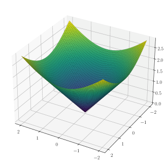
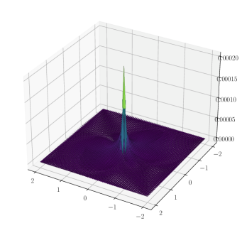
Figure 1. Plots of $\Uppi_{h_{4}}^{1}(|{\bf u}_{4}|)$ (left) and $\Uppi_{h_{4}}^{1}(|{\bf u}_{4}-{\bf u}|)$ (right) for ${p=4}$, ${\alpha=2.5}$.

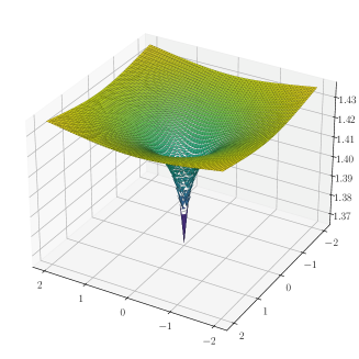
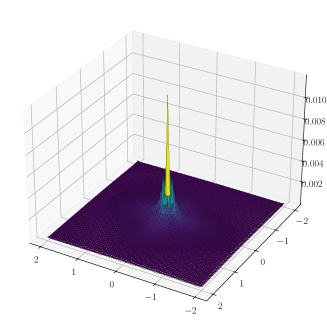
Figure 2. Plots of $\Uppi_{h_{4}}^{1}(|{\bf L}_{4}|)$ (left) and ${\Uppi_{h_{4}}^{1}(|{\bf L}_{4}-{\bf L}|)}$ (right) for ${p=4}$, ${\alpha=2.5}$.

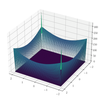
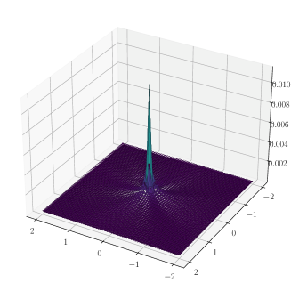
Figure 3. Plots of $\Uppi_{h_{4}}^{1}(|{\bf R}_{h_{4}}^{1}{\bf u}_{4}|)$ (left) and $\Uppi_{h_{4}}^{1}\!(|{\bf R}_{h_{4}}^{1}({\bf u}_{4}-{\bf u})|)$ (right) for ${p=4}$, ${\alpha=2.5}$.

Appendix A

This Appendix collects known results, used in the paper, and proves new results in the DG Orlicz-setting.

Lemma A.1.

Let $\psi:\mathbb{R}^{\geq 0}\to\mathbb{R}^{\geq 0}$ be an N-function satisfying the $\Delta_{2}$-condition and $k\in\mathbb{N}_{0}$. Then, for every ${\bf w}_{h}\in W^{1,\psi}(\mathcal{T}_{h})$, we have that

$$\begin{aligned} \int_{S_{\gamma}}\psi\big{(}\boldsymbol{\mathcal{R}}^{k}_{h,\gamma}{\bf w}_{h}\big{)}\,\textup{d}x&\leq c\,h\,\int_{\gamma}\psi(h^{-1}{\lvert{\llbracket{{\bf w}_{h}\otimes{\bf n}}\rrbracket}\rvert})\,\textup{d}s\,,\\ \rho_{\psi,\Omega}\big{(}\boldsymbol{\mathcal{R}}_{h}^{k}{\bf w}_{h}\big{)}&\leq c\,m_{\psi,h}({\bf w}_{h})\end{aligned}$$ (A.2)

with a constant $c>0$ depending only on $k\in\mathbb{N}_{0}$, $\Delta_{2}(\psi)>0$, and $\omega_{0}>0$.

Proof.

The assertions are proved in [17, (A.23), (A.25)]. ∎

Lemma A.3.

Let $\psi:\mathbb{R}^{\geq 0}\to\mathbb{R}^{\geq 0}$ be an N-function satisfying the $\Delta_{2}$-condition and $k\in\mathbb{N}_{0}$. Then, for every ${\bf w}_{h}\in W^{1,\psi}(\mathcal{T}_{h})$, we have that

$$c^{-1}\,M_{\psi,h}({\bf w}_{h})\leq\rho_{\psi,\Omega}\big{(}\boldsymbol{\mathcal{G}}_{h}^{k}{\bf w}_{h}\big{)}+m_{\psi,h}({\bf w}_{h})\leq c\,M_{\psi,h}({\bf w}_{h})$$ (A.4)

with a constant $c>0$ depending only on $k\in\mathbb{N}_{0}$, $\Delta_{2}(\psi)>0$, and $\omega_{0}>0$.

Proof.

The assertion follows from [17, (A.26), (A.28)] and Lemma A.1. ∎

Lemma A.5.

Let $\psi:\mathbb{R}^{\geq 0}\to\mathbb{R}^{\geq 0}$ be an N-function satisfying the $\Delta_{2}$-condition and $k\in\mathbb{N}_{0}$. Then, for every $K\in\mathcal{T}_{h}$, ${\bf u}\in W^{\ell,\psi}(K)$ and $0\leq j\leq\ell\leq k+1$, we have that

$$\mathop{\mathchoice{{\vbox{\hbox{$\textstyle-$}}\kern-4.86108pt}}{{\vbox{\hbox{$\scriptstyle-$}}\kern-3.25pt}}{{\vbox{\hbox{$\scriptscriptstyle-$}}\kern-2.29166pt}}{{\vbox{\hbox{$\scriptscriptstyle-$}}\kern-1.875pt}}\!\int}_{K}\psi\big{(}h_{K}^{j}|\nabla^{j}({\bf u}-{\Uppi_{h}^{k}}{\bf u})|\big{)}\,\textup{d}x \leq c\,\mathop{\mathchoice{{\vbox{\hbox{$\textstyle-$}}\kern-4.86108pt}}{{\vbox{\hbox{$\scriptstyle-$}}\kern-3.25pt}}{{\vbox{\hbox{$\scriptscriptstyle-$}}\kern-2.29166pt}}{{\vbox{\hbox{$\scriptscriptstyle-$}}\kern-1.875pt}}\!\int}_{K}\psi\big{(}h_{K}^{\ell}|\nabla^{\ell}{\bf u}|\big{)}\,\textup{d}x\,,$$ (A.6)

$$\mathop{\mathchoice{{\vbox{\hbox{$\textstyle-$}}\kern-4.86108pt}}{{\vbox{\hbox{$\scriptstyle-$}}\kern-3.25pt}}{{\vbox{\hbox{$\scriptscriptstyle-$}}\kern-2.29166pt}}{{\vbox{\hbox{$\scriptscriptstyle-$}}\kern-1.875pt}}\!\int}_{K}\psi\big{(}h_{K}^{j}|\nabla^{j}{\Uppi_{h}^{k}}{\bf u}|\big{)}\,\textup{d}x \leq c\,\mathop{\mathchoice{{\vbox{\hbox{$\textstyle-$}}\kern-4.86108pt}}{{\vbox{\hbox{$\scriptstyle-$}}\kern-3.25pt}}{{\vbox{\hbox{$\scriptscriptstyle-$}}\kern-2.29166pt}}{{\vbox{\hbox{$\scriptscriptstyle-$}}\kern-1.875pt}}\!\int}_{K}\psi\big{(}h_{K}^{\ell}|\nabla^{\ell}{\bf u}|\big{)}\,\textup{d}x$$ (A.7)

with a constant $c>0$ depending only on $\ell,k\in\mathbb{N}_{0}$, $\Delta_{2}(\psi)>0$, and $\omega_{0}>0$.

Proof.

The first assertion is shown in [17, (A.7)], and the second one follows from the triangle inequality. ∎

Corollary A.8.

Let $\psi:\mathbb{R}^{\geq 0}\to\mathbb{R}^{\geq 0}$ be an N-function satisfying the $\Delta_{2}$-condition and $k\in\mathbb{N}_{0}$. Then, for every ${\bf u}\in L^{\psi}(\Omega)$ and ${\bf w}_{h}\in W^{1,\psi}(\mathcal{T}_{h})$, we have that

$$\rho_{\psi,\Omega}\big{(}{\bf u}-{\Uppi_{h}^{k}}{\bf u}\big{)} \leq c\,\rho_{\psi,\Omega}({\bf u})\,,$$ (A.9)

$$\rho_{\psi,\Omega}\big{(}{\bf w}_{h}-{\Uppi_{h}^{k}}{\bf w}_{h}\big{)} \leq c\,\rho_{\psi,\Omega}(h\,{\nabla_{h}{\bf w}_{h}})\,,$$ (A.10)

$$\rho_{\psi,\Omega}\big{(}\nabla_{h}{\bf w}_{h}-\nabla_{h}{\Uppi_{h}^{k}}{\bf w}_{h}\big{)} \leq c\,\rho_{\psi,\Omega}({\nabla_{h}{\bf w}_{h}})$$ (A.11)

with a constant $c>0$ depending only on $k\in\mathbb{N}_{0}$, $\Delta_{2}(\psi)>0$, and $\omega_{0}>0$. In particular, this implies for every $k\in\mathbb{N}_{0}$, ${\bf u}\in L^{\psi}(\Omega)$ and ${\bf w}_{h}\in W^{1,\psi}(\mathcal{T}_{h})$ that

$$\rho_{\psi,\Omega}\big{(}{\Uppi_{h}^{k}}{\bf u}\big{)} \leq c\,\rho_{\psi,\Omega}({\bf u})\,,$$ (A.12)

$$\rho_{\psi,\Omega}\big{(}\nabla_{h}{\Uppi_{h}^{k}}{\bf w}_{h}\big{)} \leq c\,\rho_{\psi,\Omega}(\nabla_{h}{\bf w}_{h})\,.$$ (A.13)

For every $k\in\mathbb{N}$ and ${\bf w}_{h}\in W^{2,\psi}(\mathcal{T}_{h})$, we have that

$$\rho_{\psi,\Omega}\big{(}\nabla_{h}{\bf w}_{h}-\nabla_{h}{\Uppi_{h}^{k}}{\bf w}_{h}\big{)} \leq c\,\rho_{\psi,\Omega}\big{(}{h\nabla^{2}_{h}{\bf w}_{h}}\big{)}$$ (A.14)

with a constant $c>0$ depending only on $k\in\mathbb{N}$, $\Delta_{2}(\psi)>0$, and $\omega_{0}>0$.

Lemma A.15.

Let $\boldsymbol{\mathcal{A}}$ satisfy Assumption 2.7 for a balanced N-function ${\varphi}$ and ${k\in\mathbb{N}}$. Let ${\bf F}(\nabla{\bf u})\in W^{1,2}(\Omega)$, then

$${\big{\lVert}{{\bf F}\big{(}\nabla_{h}{\Uppi_{h}^{k}}{\bf u}\big{)}-{\bf F}(\nabla{\bf u})}\big{\rVert}}_{2}^{2} \leq c\,h^{2}\,{\lVert{\nabla{\bf F}(\nabla{\bf u})}\rVert}_{2}^{2}$$

with $c\!>\!0$ depending only on the characteristics of $\boldsymbol{\mathcal{A}}$ and $\varphi$, and the chunkiness $\omega_{0}$. The same assertion also holds for the Scott–Zhang interpolation operator ${\Uppi^{k}_{{\rm SZ}}}$.

Proof.

The assertion is proved in [18, Corollary 5.8]. ∎

Lemma A.16.

Let $\psi$ be an N-function satisfying the $\Delta_{2}$-condition and $k\in\mathbb{N}_{0}$. Let $K\in\mathcal{T}_{h}$ and $\gamma$ be a face of $K$. Then, for every ${\bf u}\in W^{1,\psi}(K)$ and ${{\bf u}_{h}\in\mathcal{P}_{k}(K)}$, it holds

$$\mathop{\mathchoice{{\vbox{\hbox{$\textstyle-$}}\kern-4.86108pt}}{{\vbox{\hbox{$\scriptstyle-$}}\kern-3.25pt}}{{\vbox{\hbox{$\scriptscriptstyle-$}}\kern-2.29166pt}}{{\vbox{\hbox{$\scriptscriptstyle-$}}\kern-1.875pt}}\!\int}_{\gamma}\psi({\lvert{{\bf u}}\rvert})\,\textup{d}s \leq c\mathop{\mathchoice{{\vbox{\hbox{$\textstyle-$}}\kern-4.86108pt}}{{\vbox{\hbox{$\scriptstyle-$}}\kern-3.25pt}}{{\vbox{\hbox{$\scriptscriptstyle-$}}\kern-2.29166pt}}{{\vbox{\hbox{$\scriptscriptstyle-$}}\kern-1.875pt}}\!\int}_{K}\psi({\lvert{{\bf u}}\rvert})\,\textup{d}x+c\mathop{\mathchoice{{\vbox{\hbox{$\textstyle-$}}\kern-4.86108pt}}{{\vbox{\hbox{$\scriptstyle-$}}\kern-3.25pt}}{{\vbox{\hbox{$\scriptscriptstyle-$}}\kern-2.29166pt}}{{\vbox{\hbox{$\scriptscriptstyle-$}}\kern-1.875pt}}\!\int}_{K}\psi(h{\lvert{\nabla{\bf u}}\rvert})\,\textup{d}x\,,$$ (A.17)

$$\mathop{\mathchoice{{\vbox{\hbox{$\textstyle-$}}\kern-4.86108pt}}{{\vbox{\hbox{$\scriptstyle-$}}\kern-3.25pt}}{{\vbox{\hbox{$\scriptscriptstyle-$}}\kern-2.29166pt}}{{\vbox{\hbox{$\scriptscriptstyle-$}}\kern-1.875pt}}\!\int}_{\gamma}\psi({\lvert{{\bf u}_{h}}\rvert})\,\textup{d}s \leq c\,\mathop{\mathchoice{{\vbox{\hbox{$\textstyle-$}}\kern-4.86108pt}}{{\vbox{\hbox{$\scriptstyle-$}}\kern-3.25pt}}{{\vbox{\hbox{$\scriptscriptstyle-$}}\kern-2.29166pt}}{{\vbox{\hbox{$\scriptscriptstyle-$}}\kern-1.875pt}}\!\int}_{K}\psi({\lvert{{\bf u}_{h}}\rvert})\,\textup{d}x\,,$$ (A.18)

with constants $c>0$ depending only on $k\in\mathbb{N}_{0}$, $\Delta_{2}(\psi)>0$, and $\omega_{0}>0$.

Proof.

The assertions are proved in [17, (A.13), (A.14)]. ∎

Corollary A.19.

Let $\psi:\mathbb{R}^{\geq 0}\to\mathbb{R}^{\geq 0}$ be an N-function satisfying the $\Delta_{2}$-condition and $k\in\mathbb{N}_{0}$. Let $K\in\mathcal{T}_{h}$ and $\gamma$ be a face of $K$. Then, for every ${\bf u}\in W^{1,\psi}(K)$, ${\bf w}_{h}\in W^{1,\psi}(\mathcal{T}_{h})$ and ${\bf u}_{h}\in U_{h}^{k}$, we have that

$$h\int_{\gamma}\psi\big{(}h^{-1}{\big{\lvert}{{\bf u}-{\Uppi_{h}^{k}}{\bf u}}\big{\rvert}}\big{)}\,\textup{d}s \leq c\int_{K}\psi({\lvert{\nabla{\bf u}}\rvert})\,\textup{d}x\,,$$ (A.20)

$$m_{\psi,h}\big{(}{\bf w}_{h}-{\Uppi_{h}^{k}}{\bf w}_{h}\big{)} \leq c\,\rho_{\psi,\Omega}(\nabla_{h}{\bf w}_{h})\,,$$ (A.21)

$$m_{\psi,h}({\bf w}_{h}) \leq c\,\rho_{\psi,\Omega}\big{(}h^{-1}{\bf w}_{h}\big{)}+c\,\rho_{\psi,\Omega}(\nabla_{h}{\bf w}_{h})\,,$$ (A.22)

$$h\,\rho_{\psi,\smash{\Gamma_{h}^{i}}\cup\Gamma_{D}}(\{{{\bf u}_{h}}\}) \leq c\,\rho_{\psi,\Omega}({\bf u}_{h})\,,$$ (A.23)

$$h\,\rho_{\psi,\smash{\Gamma_{h}^{i}}\cup\Gamma_{D}}(\{{{\bf w}_{h}-{\Uppi_{h}^{k}}{\bf w}_{h}}\}) \leq c\,\rho_{\psi,\Omega}(h\nabla_{h}{\bf w}_{h})\,,$$ (A.24)

with constants $c>0$ depending only on $k\in\mathbb{N}_{0}$, $\Delta_{2}(\psi)$, and $\omega_{0}>0$.

Proof.

For the assertions (A.20) and (A.21), we refer to [17, (A.15) & (A.16)]. The assertions (A.22) and (A.23) follow from (A.17) and (A.18), resp., by summation, while (A.24) follows from (A.20) by summation. ∎

Corollary A.25.

Let $\boldsymbol{\mathcal{A}}$ satisfy Assumption 2.7 for a balanced N-function ${\varphi}$ and $k\in\mathbb{N}_{0}$. Moreover, let ${\bf u}\in W^{1,\varphi}(\Omega)$ satisfy ${\bf F}(\nabla{\bf u})\in W^{1,2}(\Omega)$. Then, for every ${\bf w}_{h}\in W^{1,\varphi}(\mathcal{T}_{h})$, it holds

$$m_{\varphi_{{\lvert{\nabla{\bf u}}\rvert}},h}\big{(}{\bf w}_{h}-{\Uppi_{h}^{k}}{\bf w}_{h}\big{)}\leq c\,\rho_{\varphi_{{\lvert{\nabla{\bf u}}\rvert}},\Omega}(\nabla_{h}{\bf w}_{h})+c\,h^{2}\,\|\nabla{\bf F}(\nabla{\bf u})\|_{2}^{2}\,,$$ (A.26)

with constants $c>0$ depending only on $k\in\mathbb{N}_{0}$, the characteristics of $\boldsymbol{\mathcal{A}}$ and $\varphi$, and $\omega_{0}>0$.

Proof.

Using the convexity of $\varphi_{{\lvert{\nabla{\bf u}}\rvert}}$, twice a change of shift (cf. Lemma 2.15), Proposition 2.17, the local trace inequalities (A.20) and (A.17) and Poincaré’s inequality on $K$ together with [6, Lemma A.12] we find that

$$h\int_{\gamma}\varphi_{{\lvert{\nabla{\bf u}}\rvert}}\big{(}h^{-1}{\lvert{\llbracket{({\bf w}_{h}-{\Uppi_{h}^{k}}{\bf w}_{h})\otimes{\bf n}}\rrbracket}\rvert}\big{)}\,\textup{d}s$$

$$\leq h\sum_{K\in\mathcal{T}_{h};K\subseteq S_{\gamma}}{\int_{\gamma}{\varphi_{{\lvert{\langle{\nabla{\bf u}}\rangle_{K}}\rvert}}\big{(}h^{-1}{\lvert{{\bf w}_{h}-({\Uppi_{h}^{k}}{\bf w}_{h})|_{K}}\rvert}\big{)}+{\lvert{{\bf F}(\nabla{\bf u})-{\bf F}(\langle{\nabla{\bf u}}\rangle_{K})}\rvert}^{2}\,\textup{d}s}}$$

$$\leq\sum_{K\in\mathcal{T}_{h};K\subseteq S_{\gamma}}{\int_{K}{\varphi_{{\lvert{\langle{\nabla{\bf u}}\rangle_{K}}\rvert}}\big{(}|\nabla{\bf w}_{h}|\big{)}\,\textup{d}s}}+h^{2}\sum_{K\in\mathcal{T}_{h};K\subseteq S_{\gamma}}{\int_{K}{{\lvert{\nabla{\bf F}(\nabla{\bf u})}\rvert}^{2}\,\textup{d}s}}$$

$$\leq\int_{S_{\gamma}}{\varphi_{{\lvert{\nabla{\bf u}}\rvert}}\big{(}|\nabla_{h}{\bf w}_{h}|\big{)}\,\textup{d}s}+h^{2}\int_{S_{\gamma}}{{\lvert{\nabla{\bf F}(\nabla{\bf u})}\rvert}^{2}\,\textup{d}s}\,.$$

Then, the assertion follows by summing with respect to $\gamma\in\smash{\Gamma_{h}^{i}}\cup\Gamma_{D}$. ∎

Lemma A.27.

Let $\psi:\mathbb{R}^{\geq 0}\to\mathbb{R}^{\geq 0}$ be an N-function satisfying the $\Delta_{2}$-condition and $k\in\mathbb{N}$. Then, for every ${\bf u}\in W^{1,\psi}(\Omega)$, we have that

$$\rho_{\psi,\Omega}\big{(}\nabla_{h}({\Uppi_{h}^{k}}{\bf u}-{\bf u})\big{)} \to 0 \quad(h\to 0)\,,$$ (A.28)

$$m_{\psi,\Omega}\big{(}{\Uppi_{h}^{k}}{\bf u}-{\bf u}\big{)} \to 0 \quad(h\to 0)\,,$$ (A.29)

$$\rho_{\psi,\Omega}\big{(}\boldsymbol{\mathcal{R}}_{h}^{k}({\Uppi_{h}^{k}}{\bf u}-{\bf u})\big{)} \to 0 \quad(h\to 0)\,,$$ (A.30)

$$\rho_{\psi,\Omega}\big{(}\boldsymbol{\mathcal{G}}_{h}^{k}({\Uppi_{h}^{k}}{\bf u}-{\bf u})\big{)} \to 0 \quad(h\to 0)\,.$$ (A.31)

Proof.

For every ${\bf u}\in W^{1,\psi}(\Omega)$, there exists a sequence $({\bf u}^{n})_{n\in\mathbb{N}}\subseteq C^{\infty}(\overline{\Omega})$ such that

$$\rho_{\psi,\Omega}\big{(}\nabla({\bf u}^{n}-{\bf u})\big{)}\to 0\quad(n\to\infty)\,.$$ (A.32)

Thus, using (A.13), (A.14) and the properties of the N-function $\psi$, we find that

$$\begin{aligned} \rho_{\psi,\Omega}\big{(}\nabla_{h}({\Uppi_{h}^{k}}{\bf u}-{\bf u})\big{)}&\leq c\,\rho_{\psi,\Omega}\big{(}\nabla_{h}{\Uppi_{h}^{k}}({\bf u}-{\bf u}^{n})\big{)}+c\,\rho_{\psi,\Omega}\big{(}\nabla_{h}({\Uppi_{h}^{k}}{\bf u}^{n}-{\bf u}^{n})\big{)}\\ &\quad+c\,\rho_{\psi,\Omega}\big{(}\nabla({\bf u}^{n}-{\bf u})\big{)}\\ &\leq c\,\rho_{\psi,\Omega}\big{(}\nabla({\bf u}^{n}-{\bf u})\big{)}+c\,\rho_{\psi,\Omega}\big{(}h\,\nabla^{2}{\bf u}^{n}\big{)}\,.\end{aligned}$$ (A.33)

Due to (A.32), for every ${\varepsilon}>0$, there exists $n_{0}\in\mathbb{N}$ such that ${c\rho_{\psi,\Omega}(\nabla({\bf u}^{n}-{\bf u}))\!\leq\!{\varepsilon}}$ for all $n\in\mathbb{N}$ with $n\geq n_{0}$. Therefore, choosing $n=n_{0}\in\mathbb{N}$ in (A.33), we conclude that $\lim_{h\to 0}\rho_{\psi,\Omega}(\nabla_{h}({\Uppi_{h}^{k}}{\bf u}-{\bf u}))\!\leq\!{\varepsilon}$, which yields (A.28), since ${\varepsilon}\!>\!0$ was chosen arbitrarily.

Choosing ${\Uppi_{h}^{k}}{\bf u}-{\bf u}={\Uppi_{h}^{k}}{\bf u}-{\bf u}-{\Uppi_{h}^{k}}({\Uppi_{h}^{k}}{\bf u}-{\bf u})$ in (A.21), since ${W^{1,\psi}(\Omega)\subseteq W^{1,\psi}(\mathcal{T}_{h})}$, also using (A.28), we find that $m_{\psi,\Omega}({\Uppi_{h}^{k}}{\bf u}-{\bf u})\leq c\,\rho_{\psi,\Omega}(\nabla_{h}({\Uppi_{h}^{k}}{\bf u}-{\bf u}))\to 0$ ${(h\to 0)}$, which is (A.29).

Next, (A.2) and (A.29) yield $\rho_{\psi,\Omega}(\boldsymbol{\mathcal{R}}_{h}^{k}({\Uppi_{h}^{k}}{\bf u}-{\bf u}))\leq c\,m_{\psi,\Omega}({\Uppi_{h}^{k}}{\bf u}-{\bf u})\to 0$ $(h\to 0)$, which is (A.30).

Finally, (A.31) follows from the definition of $\boldsymbol{\mathcal{G}}_{h}^{k}$ in (2.40), (A.28) and (A.30). ∎

Lemma A.34.

Let $\psi:\mathbb{R}^{\geq 0}\to\mathbb{R}^{\geq 0}$ be an N-function such that $\psi$ and $\psi^{*}$ satisfy the $\Delta_{2}$-condition. Then, for every ${\bf w}_{h}\in W^{1,\psi}(\mathcal{T}_{h})$, we have that

$$\rho_{\psi,\Omega}({\bf w}_{h}) \leq c\,M_{\psi,h}(\operatorname{diam}(\Omega)\,{\bf w}_{h})\,,$$ (A.35)

$$\rho_{\psi,\Gamma_{N}}({\bf w}_{h}) \leq c\,\operatorname{diam}(\Omega)^{-1}M_{\psi,h}(\operatorname{diam}(\Omega)\,{\bf w}_{h})\,,$$ (A.36)

where $c>0$ only depends on $\Omega,\Omega^{\prime}\subseteq\mathbb{R}^{n}$, $n\geq 2$, and $\Delta_{2}(\psi),\Delta_{2}(\psi^{*}),\omega_{0}>0$.

Proof.

This is proved in [17, Lemma A.9, Lemma A.10]. ∎

Lemma A.37.

Let $\psi:\mathbb{R}^{\geq 0}\to\mathbb{R}^{\geq 0}$ be an N-function such that $\psi$ and $\psi^{*}$ satisfy the $\Delta_{2}$-condition and $k\!\in\!\mathbb{N}$. Let ${\bf w}_{h}\!\in\!W^{1,\psi}(\mathcal{T}_{h})$, $h\!>\!0$, be such that ${\sup_{h>0}M_{\psi,h}({\bf w}_{h})\!\leq\!c}$. Then, for the sequence ${\bf w}_{n}\vcentcolon={\bf w}_{h_{n}}\in W^{1,\psi}(\mathcal{T}_{h_{n}})$, where $h_{n}\to 0$ $(n\to\infty)$, there exists a function ${\bf w}\in W^{1,\psi}_{\Gamma_{D}}(\Omega)$ such that, up to subsequences, we have that

$${\bf w}_{n} \rightharpoonup{\bf w} \quad\text{ in }L^{\psi}(\Omega) \quad(n\to\infty)\,,$$ (A.38)

$$\boldsymbol{\mathcal{G}}_{h_{n}}^{k}{\bf w}_{n} \rightharpoonup\nabla{\bf w} \quad\text{ in }L^{\psi}(\Omega) \quad(n\to\infty)\,,$$ (A.39)

$${\bf w}_{n} \rightharpoonup{\bf w} \quad\text{ in }L^{\psi}(\Gamma_{N}) \quad(n\to\infty)\,.$$ (A.40)

Proof.

The proof is a straightforward adaptation of the proof of [13, Theorem 5.7]. In fact, from Poincaré’s inequality (A.35) and the reflexivity of $L^{\psi}(\Omega)$, it follows that there exists ${\bf w}\in L^{\psi}(\Omega)$ such that for a not relabeled subsequence, it holds (A.38). We extend both ${\bf w}$ and ${\bf w}_{n}$ by zero to $\Omega^{\prime}\setminus\Omega$ and denote the extensions again by ${\bf w}$ and ${\bf w}_{n}$, respectively. Moreover, we extend $\smash{\boldsymbol{\mathcal{R}}_{h_{n}}^{k}{\bf w}_{n}}$ by zero to $\Omega^{\prime}\setminus\Omega$ and denote the extension again by $\smash{\boldsymbol{\mathcal{R}}_{h_{n}}^{k}{\bf w}_{n}}$. Using these extensions and (A.4), we obtain a not relabeled sub-sequence and a function ${\bf G}\in L^{\psi}(\Omega^{\prime})$ such that

$$\boldsymbol{\mathcal{G}}_{h_{n}}^{k}{\bf w}_{n} \rightharpoonup{\bf H}\quad\text{ in }L^{\psi}(\Omega^{\prime})\quad(n\to\infty)\,.$$ (A.41)

We have to show that ${\bf H}=\nabla{\bf w}$ holds in $L^{\psi}(\Omega^{\prime})$. To this end, we observe that for every ${\bf X}\in C^{\infty}_{0}(\Omega^{\prime})$, there holds

$$\begin{aligned} \big{(}\boldsymbol{\mathcal{G}}_{h_{n}}^{k}{\bf w}_{n},{\bf X}\big{)}_{\Omega^{\prime}}&=\big{(}\nabla_{h_{n}}{\bf w}_{n},{\bf X}\big{)}_{\Omega^{\prime}}-\big{(}\boldsymbol{\mathcal{R}}_{h_{n}}^{k}{\bf w}_{n},\Uppi_{h_{n}}^{k}{\bf X}\big{)}_{\Omega^{\prime}}\\ &=-({\bf w}_{n},\operatorname{div}{\bf X})_{\Omega^{\prime}}+\big{\langle}\llbracket{\bf w}_{n}\otimes{\bf n}\rrbracket,\big{\{}{\bf X}-\Uppi_{h_{n}}^{k}{\bf X}\big{\}}\big{\rangle}_{\smash{\smash{\Gamma_{h}^{i}}^{\prime}\cup\Gamma_{D}^{\prime}}}\,.\end{aligned}$$ (A.42)

Using Young’s inequality, $\sup_{n\in\mathbb{N}}{m_{\psi,h_{n}}({\bf w}_{n})}\leq\sup_{n\in\mathbb{N}}{M_{\psi,h_{n}}({\bf w}_{n})}<\infty$ and (A.21) for $\psi^{*}$, by passing for $n\to\infty$, for every ${\bf X}\in C^{\infty}_{0}(\Omega^{\prime})$, we find that

$$\big{\langle}\llbracket{\bf w}_{n}\otimes{\bf n}\rrbracket,\big{\{}{\bf X}-\Uppi_{h_{n}}^{k}{\bf X}\big{\}}\big{\rangle}_{\smash{\smash{\Gamma_{h}^{i}}^{\prime}\cup\Gamma_{D}^{\prime}}}\leq h_{n}c\big{(}m_{\psi^{*},h_{n}}\big{(}{\bf X}-\Uppi_{h_{n}}^{k}{\bf X}\big{)}+m_{\psi,h_{n}}({\bf w}_{n})\big{)}\to 0\,.$$

Thus, by passing for $n\!\to\!\infty$ in (A.42), using (A.41) and (A.38), for any ${{\bf X}\in C^{\infty}_{0}(\Omega^{\prime})}$, we arrive at $({\bf H},{\bf X})_{\Omega^{\prime}}=-({\bf w},\operatorname{div}{\bf X})_{\Omega^{\prime}}$, i.e., ${\bf H}=\nabla{\bf w}$ in $\Omega^{\prime}$ and, thus, ${\bf w}\in W^{1,\psi}(\Omega^{\prime})$. Since ${\bf w}={\mathbf{0}}$ in $\Omega^{\prime}\setminus\Omega$, we get ${{\bf w}\in W^{1,\psi}_{\Gamma_{D}}(\Omega)}$.

Inequality (A.36) and the reflexivity of $L^{\psi}(\Gamma_{N})$ yield a not relabeled subsequence and a function ${\bf g}\in L^{\psi}(\Gamma_{N})$ such that

$${\bf w}_{n} \rightharpoonup{\bf h}\quad\text{ in }L^{\psi}(\Gamma_{N})\quad(n\to\infty)\,.$$ (A.43)

Similar arguments as above yield that for every ${\bf X}\in C^{\infty}(\overline{\Omega})$, we have that

$$\big{(}\boldsymbol{\mathcal{G}}_{h_{n}}^{k}{\bf w}_{n},{\bf X}\big{)}_{\smash{\Omega}} \!=\!-({\bf w}_{n},\operatorname{div}{\bf X})_{\Omega}\!+\!\big{\langle}\llbracket{\bf w}_{n}\otimes{\bf n}\rrbracket,\!\big{\{}{\bf X}-\Uppi_{h_{n}}^{k}{\bf X}\big{\}}\big{\rangle}_{\smash{\smash{\Gamma_{h}^{i}}\cup\Gamma_{D}}}\!+\!\langle{\bf w}_{n}\otimes{\bf n},{\bf X}\rangle_{\Gamma_{N}}.$$

Taking the limit with respect to $n\to\infty$ in this equality, we find that

$$(\nabla{\bf w},{\bf X})_{\Omega} =-\big{(}{\bf w},\operatorname{div}{\bf X})_{\Omega}+\langle{\bf h}\otimes{\bf n},{\bf X}\rangle_{\Gamma_{N}}$$

$$=(\nabla{\bf w},{\bf X})_{\Omega}+\langle({\bf h}-{\bf w})\otimes{\bf n},{\bf X}\rangle_{\Gamma_{N}}\,.$$

Choosing ${\bf X}={\bf z}\otimes{\bf n}$ for arbitrary ${\bf z}\in C^{\infty}_{0}(\Gamma_{N})$, we conclude that ${\bf h}={\bf w}$ in $L^{\psi}(\Gamma_{N})$, which together with (A.43) proves (A.40). ∎

References

- [1] E. Acerbi and N. Fusco, Regularity for minimizers of nonquadratic functionals: the case , J. Math. Anal. Appl. 140 (1989), no. 1, 115–135.
- [2] D. N. Arnold, F. Brezzi, B. Cockburn, and L. D. Marini, Unified analysis of discontinuous Galerkin methods for elliptic problems, SIAM J. Numer. Anal. 39 (2001/02), no. 5, 1749–1779.
- [3] S. Balay et al., PETSc Web page, https://www.mcs.anl.gov/petsc, 2019.
- [4] J. W. Barrett and W. B. Liu, Quasi-norm error bounds for the finite element approximation of a non-Newtonian flow, Numer. Math. 68 (1994), no. 4, 437–456.
- [5] S. Bartels, Nonconforming discretizations of convex minimization problems and precise relations to mixed methods, Comput. Math. Appl. 93 (2021), 214–229.
- [6] L. Belenki, L. C. Berselli, L. Diening, and M. Růžička, On the Finite Element Approximation of -Stokes Systems, SIAM J. Numer. Anal. 50 (2012), no. 2, 373–397.
- [7] L. Belenki, L. Diening, and C. Kreuzer, Optimality of an adaptive finite element method for the -Laplacian equation, IMA J. Numer. Anal. 32 (2012), no. 2, 484–510.
- [8] L. C. Berselli and M. Růžička, Natural second-order regularity for parabolic systems with operators having -structure and depending only on the symmetric gradient, Calc. Var. PDEs (2022), Paper No. 137.
- [9] D. Breit and A. Cianchi, Negative Orlicz-Sobolev norms and strongly nonlinear systems in fluid mechanics, J. Differential Equations 259 (2015), no. 1, 48–83.
- [10] A. Buffa and C. Ortner, Compact embeddings of broken Sobolev spaces and applications, IMA J. Numer. Anal. 29 (2009), no. 4, 827–855.
- [11] E. Burman and A. Ern, Discontinuous Galerkin approximation with discrete variational principle for the nonlinear Laplacian, C. R. Math. Acad. Sci. Paris 346 (2008), no. 17-18, 1013–1016.
- [12] B. Cockburn and J. Shen, A Hybridizable Discontinuous Galerkin Method for the -Laplacian, SIAM Journal on Scientific Computing 38 (2016), no. 1, A545–A566.
- [13] D.A. Di Pietro and A. Ern, Mathematical aspects of discontinuous Galerkin methods, Mathématiques & Applications, vol. 69, Springer, Berlin, 2012.
- [14] L. Diening and F. Ettwein, Fractional estimates for non-differentiable elliptic systems with general growth, Forum Math. 20 (2008), no. 3, 523–556.
- [15] L. Diening, M. Fornasier, R. Tomasi, and M. Wank, A relaxed Kačanov iteration for the -Poisson problem, Numer. Math. 145 (2020), no. 1, 1–34.
- [16] L. Diening, C. Kreuzer, and S. Schwarzacher, Convex hull property and maximum principle for finite element minimisers of general convex functionals, Numer. Math. 124 (2013), no. 4, 685–700.
- [17] L. Diening, D. Kröner, M. Růžička, and I. Toulopoulos, A Local Discontinuous Galerkin approximation for systems with -structure, IMA J. Num. Anal. 34 (2014), no. 4, 1447–1488.
- [18] L. Diening and M. Růžička, Interpolation Operators in Orlicz–Sobolev Spaces, Num. Math. 107 (2007), 107–129.
- [19] C. Ebmeyer and W. B. Liu, Quasi-Norm Interpolation Error Estimates for Finite Element Approximations of Problems with –Structure, Numer. Math. 100 (2005), 233–258.
- [20] E. Emmrich and A. Wróblewska-Kamińska, Convergence of a full discretization of quasi-linear parabolic equations in isotropic and anisotropic Orlicz spaces, SIAM J. Numer. Anal. 51 (2013), no. 2, 1163–1184.
- [21] J. D. Hunter, Matplotlib: A 2D graphics environment, Computing in Science & Engineering 9 (2007), no. 3, 90–95.
- [22] A. Logg and G. N. Wells, DOLFIN: Automated Finite Element Computing, ACM Transactions on Mathematical Software 37 (2010), no. 2, 1–28.
- [23] T. Malkmus, M. Růžička, S. Eckstein, and I. Toulopoulos, Generalizations of SIP methods to systems with -structure, IMA J. Numer. Anal. 38 (2018), no. 3, 1420–1451.
- [24] G. Palmieri, Some inequalities for intermediate derivatives in Orlicz-Sobolev spaces, and applications, Rend. Accad. Sci. Fis. Mat. Napoli (4) 46 (1979), 633–652 (1980).
- [25] W. Qiu and K. Shi, Analysis on an HDG method for the -Laplacian equations, J. Sci. Comput. 80 (2019), no. 2, 1019–1032.
- [26] M. M. Rao and Z. D. Ren, Theory of Orlicz spaces, Monographs and Textbooks in Pure and Applied Mathematics, vol. 146, Marcel Dekker Inc., New York, 1991.
- [27] A. M. Ruf, Convergence of a full discretization for a second-order nonlinear elastodynamic equation in isotropic and anisotropic Orlicz spaces, Z. Angew. Math. Phys. 68 (2017), no. 5, Paper No. 118, 24.
- [28] M. Růžička, Analysis of generalized Newtonian fluids, Topics in mathematical fluid mechanics, Lecture Notes in Math., vol. 2073, Springer, Heidelberg, 2013, pp. 199–238.
- [29] M. Růžička and L. Diening, Non–Newtonian Fluids and Function Spaces, Nonlinear Analysis, Function Spaces and Applications, Proceedings of NAFSA 2006 Prague, vol. 8, 2007, pp. 95–144.
- [30] L. R. Scott and S. Zhang, Finite element interpolation of nonsmooth functions satisfying boundary conditions, Math. Comp. 54 (1990), no. 190, 483–493.
- [31] E. Zeidler, Nonlinear functional analysis and its applications. II/B, Springer, New York, 1990, Nonlinear monotone operators.