Spectral functions of the half-filled 1D Hubbard chain within the exchange-correlation potential formalism

Abstract

The spectral functions of the one-band half-filled 1D Hubbard chain are calculated using the exchange-correlation potential formalism developed recently. The exchange-correlation potential is adopted from the exact potential derived from the Hubbard dimer. Within an approximation in which the full Green function is replaced by a non-interacting one, the spectral functions can be calculated analytically. Despite the simplicity of the approximation, the resulting spectra are in favorable agreement with the more accurate results obtained from the dynamic density-matrix renormalization group method. In particular, the calculated band gap as a function of $U$ is in close agreement with the exact gap obtained from the Bethe ansatz. In addition, the formal general solution to the equation of motion of the Green function is presented and the difference between the traditional self-energy approach and the exchange-correlation potential formalism is also discussed and elaborated. A simplified Holstein Hamiltonian is considered to further illustrate the general form of the exchange-correlation potential.

I Introduction

Very recently, a completely different route for calculating the Green function was proposed. The formalism replaces the traditional self-energy by a time-dependent exchange-correlation potential, $V_{\mathrm{xc}}(r,r^{\prime};t)$, which acts as a multiplicative potential on the Green function, in contrast to the self-energy which acts as a convolution in space and time aryasetiawan2022 .

In this previous work, the formalism was illustrated by deriving the exact $V_{\mathrm{xc}}$ of the Hubbard dimer expressed in the site orbitals. In this paper, the formalism is applied to calculate the Green function of the one-dimensional Hubbard chain at half filling by utilizing the $V_{\mathrm{xc}}$ derived from the Hubbard dimer, rewritten in the bonding and anti-bonding orbitals appropriate for extension to the one-dimensional chain. Under certain approximations, the Green function can be calculated analytically, providing explicit insights into the dependence of the spectra on the parameters of the model. Despite the simple appearance of the Hamiltonian of the one-dimensional Hubbard chain, it is actually a rather stringent test for a many-electron theory. It is well known that the exact solution based on the Bethe ansatz yields two branches of collective excitations corresponding to the holon and the spinon giamarchi2004 ; essler2005 . While the Bethe-ansatz solution provides the dispersion of the holon and the spinon, it does not contain information about the spectral distribution. The spectral functions, however, have been calculated within the dynamical density-matrix renormalization group method benthien2007 and furnish comparison with the present work. Earlier calculations are limited to the large $U$ limit sorella1992 ; penc1996 and there are also related investigations on Luttinger liquid meden1992 ; voit1993 . The 1D Hubbard model is physically relevant as shown, for example, in the case of SrCuO₂, which has been found to exhibit the spinon and holon excitations kim1996 ; kim1997 .

Apart from application to the 1D Hubbard chain, a formal solution of the equation of motion of the Green function is derived, which provides an iterative scheme in practical calculations.

To contrast the traditional self-energy approach and the exchange-correlation formalism, comparison between the two is made and discussed from a historical perspective and the differences are emphasized and elaborated.

In addition, the exchange-correlation potential of a simplified Holstein Hamiltonian, describing a coupling between a core electron and a set of bosons (e.g., plasmons or phonons) is derived analytically and serves as a further illustration of the exchange-correlation potential formalism. This sheds lights on the form of $V_{\mathrm{xc}}$, which offers a very simple physical interpretation.

II Theory

The exchange-correlation potential formalism developed in the previous work aryasetiawan2022 is summarized and the main results are presented.

II.1 Equation of motion of the Green function

The zero-temperature time-ordered Green function is defined as fetter

$$iG(rt,r^{\prime}t^{\prime})=\left\langle T[\hat{\psi}(rt)\hat{\psi}^{{\dagger}}(r^{\prime}t^{\prime})]\right\rangle,$$ (1)

where $r=(\mathbf{r},\sigma)$ labels both space and spin variables, $\hat{\psi}(rt)$ is the Heisenberg field operator, $T$ is the time-ordering symbol, and $\left\langle...\right\rangle$ denotes expectation value in the ground state. Extension to finite temperature is quite straightforward. The many-electron Hamiltonian defining the Heisenberg operator is given by

$$\hat{H} =\int dr\;\hat{\psi}^{{\dagger}}(r)h_{0}(r)\hat{\psi}(r)$$

$$+\frac{1}{2}\int drdr^{\prime}\;\hat{\psi}^{{\dagger}}(r)\hat{\psi}^{{\dagger}}(r^{\prime})v(r-r^{\prime})\hat{\psi}(r^{\prime})\hat{\psi}(r),$$ (2)

where $h_{0}=-\frac{1}{2}\nabla^{2}+V_{\mathrm{ext}}(r)$ and $v(r-r^{\prime})=1/|\mathbf{r-r}^{\prime}|$. In our notation, $\int dr=\sum_{\sigma}\int d^{3}r$ and atomic units are used throughout, in which the Bohr radius $a_{0}$, the electron mass $m_{e}$, the electronic charge $e$, and $\hbar$ are set to unity. For a system in equilibrium, the Hamiltonian is time independent and $t^{\prime}$ may be set to zero. The equation of motion of the Green function is given by

$$\left(i\frac{\partial}{\partial t}-h_{0}(r)\right)G(r,r^{\prime};t)$$

$$+i\int dr^{\prime\prime}v(r-r^{\prime\prime})\left\langle T[\hat{\rho}(r^{\prime\prime}t)\hat{\psi}(rt)\hat{\psi}^{{\dagger}}(r^{\prime})]\right\rangle$$

$$=\delta(t)\delta(r-r^{\prime}).$$ (3)

Since the Green function was conceived in the 1950’s, the traditional approach is to introduce the self-energy $\Sigma$ and truncate the hierarchy of higher-order Green functions such that fetter

$$-i\int dr^{\prime\prime}v(r-r^{\prime\prime})\left\langle T[\hat{\rho}(r^{\prime\prime}t)\hat{\psi}(rt)\hat{\psi}^{{\dagger}}(r^{\prime})]\right\rangle$$

$$=V_{\mathrm{H}}(r)G(r,r^{\prime};t)+\int dr^{\prime\prime}dt^{\prime\prime}\Sigma(r,r^{\prime\prime};t-t^{\prime\prime})G(r^{\prime\prime},r^{\prime};t^{\prime\prime}).$$ (4)

The equation of motion then becomes

$$\left(i\frac{\partial}{\partial t}-h(r)\right)G(r,r^{\prime};t)$$

$$-\int dr^{\prime\prime}dt^{\prime\prime}\Sigma(r,r^{\prime\prime};t-t^{\prime\prime})G(r^{\prime\prime},r^{\prime};t^{\prime\prime})$$

$$=\delta(r-r^{\prime})\delta(t),$$ (5)

where $h=h_{0}+V_{\mathrm{H}}$ with $V_{\mathrm{H}}$ being the Hartree potential.

As shown in the previous work aryasetiawan2022 , it is possible to define an exchange-correlation potential $V_{\mathrm{xc}}$ so that the Green function fulfills the following equation of motion:

$$\left(i\frac{\partial}{\partial t}-h(r)-V_{\mathrm{xc}}(r,r^{\prime};t)\right)G(r,r^{\prime};t)=\delta(r-r^{\prime})\delta(t),$$ (6)

where $V_{\mathrm{xc}}$ is the Coulomb potential of the time-dependent exchange-correlation hole, $\rho_{\mathrm{xc}}$:

$$V_{\mathrm{xc}}(r,r^{\prime};t)=\int dr^{\prime\prime}v(r-r^{\prime\prime})\rho_{\mathrm{xc}}(r,r^{\prime},r^{\prime\prime};t).$$ (7)

and $\rho_{\mathrm{xc}}$ is given by

$$\rho_{\mathrm{xc}}(r,r^{\prime},r^{\prime\prime};t)=[g(r,r^{\prime},r^{\prime\prime};t)-1]\rho(r^{\prime\prime}),$$ (8)

in which the correlator $g$ is defined according to

$$\left\langle T[\hat{\rho}(r^{\prime\prime}t)\hat{\psi}(rt)\hat{\psi}^{{\dagger}}(r^{\prime})]\right\rangle$$

$$=iG(r,r^{\prime};t)g(r,r^{\prime},r^{\prime\prime};t)\rho(r^{\prime\prime})$$

$$=iG(r,r^{\prime};t)[\rho(r^{\prime\prime})+\rho_{\mathrm{xc}}(r,r^{\prime},r^{\prime\prime};t)].$$ (9)

The exchange-correlation hole fulfills the sum rule

$$\int d^{3}r^{\prime\prime}\rho_{\mathrm{xc}}(r,r^{\prime},r^{\prime\prime};t)=-\delta_{\sigma\sigma^{\prime\prime}}\theta(-t)$$ (10)

and it has the property

$$\rho_{\mathrm{xc}}(r,r^{\prime},r;t)=-\rho(r)$$ (11)

for any $r,r^{\prime}$, and $t$. The sum-rule and the above property may be seen as the dynamic version of the corresponding properties of the static exchange-correlation hole becke2014 originating from the seminal work of Slater on the exchange hole slater1951 ; slater1968 . For a given $r^{\prime}$, $V_{\mathrm{xc}}(r,r^{\prime};t)$ may be interpreted as a local time-dependent one-particle potential in which the added hole/electron moves.

In the language of functional derivative technique, the exchange-correlation hole can be related to the functional derivative of the Green function with respect to a probing field $\varphi$ hedin1965 ; aryasetiawan1998 . Since

$$\left\langle T[\hat{\rho}(3)\hat{\psi}(1)\hat{\psi}^{{\dagger}}(2)]\right\rangle =i\rho(3)G(1,2)-\frac{\delta G(1,2)}{\delta\varphi(3)}$$ (12)

it follows that

$$i\rho_{\mathrm{xc}}(1,2,3)G(1,2)=-\frac{\delta G(1,2)}{\delta\varphi(3)},$$ (13)

where $1=(r_{1},t_{1})$ etc.

II.2 General iterative solution

From the equations of motion for $G$ and $G^{\mathrm{H}}$ of the Hartree approximation, a Dyson-like equation can be constructed as follows

$$G(r,r^{\prime};t)=G^{\mathrm{H}}(r,r^{\prime};t)$$

$$+\int dr^{\prime\prime}dt^{\prime}G^{\mathrm{H}}(r,r^{\prime\prime};t-t^{\prime})V_{\mathrm{xc}}(r^{\prime\prime},r^{\prime};t^{\prime})G(r^{\prime\prime},r^{\prime};t^{\prime}).$$ (14)

By operating $i\partial/\partial t-h(r)$ on both sides of the equation, it can be verified that the above $G$ fulfills the equation of motion. This Dyson-like equation can be used as an iterative scheme for solving for $G$. The iteration is started by setting $G=G^{\mathrm{H}}$ on the right-hand side and continued until self-consistency is achieved. One may choose a different starting point, such as the Kohn-Sham kohn1965 Green function $G^{\mathrm{KS}}$, in which case $V_{\mathrm{xc}}$ must be replaced with $V_{\mathrm{xc}}-V^{\mathrm{KS}}_{\mathrm{xc}}$.

In practice, it is convenient to express the equation of motion in a set of base orbitals $\{\varphi_{i}\}$:

$$i\frac{\partial}{\partial t}G_{ij}(t)-\sum_{k}h_{ik}G_{kj}(t)-\sum_{kl}V_{ik,lj}^{\mathrm{xc}}(t)G_{kl}(t)=\delta_{ij}\delta(t),$$ (15)

where $G_{ij}$ and $h_{ik}$ are the matrix elements of $G$ and $h$ in the orbitals and

$$V_{ik,lj}^{\mathrm{xc}}(t)=\int d^{3}rd^{3}r^{\prime}\;\varphi_{i}^{\ast}(r)\varphi_{k}(r)V_{\mathrm{xc}}(r,r^{\prime};t)\varphi_{l}^{\ast}(r^{\prime})\varphi_{j}(r^{\prime}).$$ (16)

The Dyson-like equation becomes

$$G_{ij}(t)=G^{\mathrm{H}}_{ij}(t)+\sum_{k}\int dt^{\prime}G^{\mathrm{H}}_{ik}(t-t^{\prime})F_{kj}(t^{\prime}),$$ (17)

in which

$$F_{kj}(t^{\prime})=\sum_{lm}V_{kl,mj}^{\mathrm{xc}}(t^{\prime})G_{lm}(t^{\prime}).$$ (18)

Fourier transformation leads to

$$G_{ij}(\omega)=G^{\mathrm{H}}_{ij}(\omega)+\sum_{k}G^{\mathrm{H}}_{ik}(\omega)F_{kj}(\omega),$$ (19)

and

$$F_{kj}(\omega)=\sum_{lm}\int\frac{d\omega^{\prime}}{2\pi}V_{kl,mj}^{\mathrm{xc}}(\omega-\omega^{\prime})G_{lm}(\omega^{\prime}).$$ (20)

This yields an integral equation for $F(\omega)$:

$$F_{kj}(\omega) =\sum_{lm}\int\frac{d\omega^{\prime}}{2\pi}V_{kl,mj}^{\mathrm{xc}}(\omega-\omega^{\prime})$$

$$\times\left[G^{\mathrm{H}}_{lm}(\omega^{\prime})+\sum_{n}G^{\mathrm{H}}_{ln}(\omega^{\prime})F_{nm}(\omega^{\prime})\right].$$ (21)

Since $G^{\mathrm{H}}$ is a non-interacting Green function, the integrals over $\omega^{\prime}$ can be performed analytically.

Alternatively, by isolating the terms containing $G_{ij}$, the equation of motion can be rewritten as follows:

$$\left\{i\frac{\partial}{\partial t}-h_{ii}-V_{ii,jj}^{\mathrm{xc}}(t)-D_{ij}(t)\right\}G_{ij}(t)=\delta_{ij}\delta(t),$$ (22)

where

$$D_{ij}(t)=\frac{1}{G_{ij}(t)}$$

$$\times\left\{\sum_{k\neq i}h_{ik}G_{kj}(t)+\sum_{k\neq i,l\neq j}V_{ik,lj}^{\mathrm{xc}}(t)G_{kl}(t)\right\}.$$ (23)

The formal iterative solution is given by

$$G_{ij}(t)=\left[G_{ij}(0^{-})\theta(-t)+G_{ij}(0^{+})\theta(t)\right]$$

$$\times\exp\left\{-i\int_{0}^{t}dt^{\prime}\left[h_{ii}+V_{ii,jj}^{\mathrm{xc}}(t^{\prime})+D_{ij}(t^{\prime})\right]\right\},$$ (24)

where

$$iG_{ij}(0^{+})-iG_{ij}(0^{-})=\delta_{ij},$$ (25)

which is obtained by integrating the equation of motion from $0^{-}$ to $0^{+}$. Since the Green function to be solved appears on the right-hand side of the equation, the formal solution in Eq. (24) facilitates an iterative scheme for solving the Green function.

II.3 Self-energy $vs.$ exchange-correlation potential

A fundamental difference between the traditional self-energy and the exchange-correlation potential approaches is that the former acts on the Green function as a convolution in space and time whereas the latter acts multiplicatively. The multiplicative property of $V_{\mathrm{xc}}$ has consequences. One of these is that the equation of motion in Eq. (6) separates into the equation for the hole Green function $(t<0)$ and for the electron Green function $(t>0)$. In contrast, due to the convolution in time in the self-energy term, solving for the hole Green function using the equation of motion in Eq. (5) requires explicit knowledge of the electron Green function and vice versa. On the other hand, the self-energy formalism is advantageous when expressed in frequency space since the Dyson equation can be solved for each frequency whereas the exchange-correlation potential formalism involves a convolution in frequency. Thus, the two approaches complement one another.

It was recently shown for the half-filled one-band Hubbard model in a square lattice that the use of the self-energy, calculated to a finite order of expansion in the interaction, to determine the Green function via the Dyson equation can lead to incorrect physics mcniven2021 . While a direct expansion of the Green function to the same order yields an insulating behavior, the Green function obtained from the Dyson equation results in a metallic behavior. This discrepancy can be traced back to the reducible diagrams implicitly summed when solving the Dyson equation, which generally differ from those in the direct expansion of the Green function at each order. This finding raises questions on the appropriateness of using the Dyson equation. The exchange-correlation potential formalism, on the other hand, is not meant to rely upon many-body perturbation theory but rather on direct construction based on known exact or accurate results of model systems and on exact properties of the exchange-correlation hole.

The choice of the self-energy as a truncation scheme may be understandable from historical perspective. In the 1950’s and early 1960’s it was presumably inconceivable to even consider many-body calculations on real materials. The commonly used model of solids at that time was the electron gas. For the electron gas, the definition of the self-energy acting on the Green function as a convolution in space and time has a great advantage in that it allows for a simple expression for the equation of motion or the Dyson equation when Fourier transformed:

$$G(k,\omega)=G_{0}(k,\omega)+G_{0}(k,\omega)\Sigma(k,\omega)G(k,\omega),$$ (26)

where $G_{0}$ is the Green function of the free-electron gas. The self-energy has since then been synonymous with the Green function and become the accepted route for calculating the Green function to this day.

The important role that the self-energy has played in electronic structure theory is not to be undermined. In the self-energy formalism an iterative equation for the self-energy can be derived yielding hedin1965 ; aryasetiawan1998

$$\Sigma(1,2) =i\int d3d4v(1-3)G(1,4)$$

$$\times\left[\left\{\delta(4-3)+\frac{\delta V_{\mathrm{H}}(4)}{\delta\phi(3)}\right\}\delta(4-2)+\frac{\delta\Sigma(4,2)}{\delta\phi(3)}\right].$$ (27)

Here, $1=(r_{1}t_{1})$ etc. and $\phi$ is a probing field which is set to zero after the derivative is taken. Neglecting the term $\delta\Sigma/\delta\phi$ leads to the well-known $GW$ approximation. This kind of iterative or perturbative equation is more difficult to establish for $V_{\mathrm{xc}}$ since the equation of motion in Eq. (6) cannot be easily inverted to obtain $G^{-1}$.

From the definition of the self-energy in Eq. (4), it can be seen that the Coulomb interaction has been lumped into the self-energy. While it is formally and mathematically correct, the definition makes no use of the fact that the Coulomb interaction is known explicitly. The definition of the correlator $g$ in Eq. (9), on the other hand, is independent of the Coulomb interaction. The special property of the Coulomb interaction being dependent only on the distance between two electrons can be exploited leading to the conclusion that only the spherical average of the exchange-correlation hole is relevant gunnarsson1976 ; jones1989 . This should greatly simplify the search for a good approximation for the exchange-correlation hole or potential.

III Model systems

To illustrate the form of the time-dependent exchange-correlation potential, the half-filled Hubbard dimer is considered. The exchange-correlation potential extracted from the Hubbard dimer is then used as an approximate $V_{\mathrm{xc}}$ for the 1D Hubbard chain.

Another example is a simplified Holstein model, describing a core electron coupled to a set of bosons such as plasmons or phonons. This Hamiltonian is appropriate to model solids in which the valence electrons are relatively delocalized, resembling electron gas. The alkalis and $s$-$p$ semiconductors and insulators are examples of such systems.

The fourth example is the hydrogen atom. Although it is not a many-electron system it illustrates explicitly the sum rule and condition fulfilled by the exchange-correlation hole.

III.1 Hubbard dimer

In the previous paper aryasetiawan2022 , the exchange-correlation potential of the half-filled Hubbard dimer was worked out analytically. The Hamiltonian of the Hubbard dimer in standard notation is given by

$$\hat{H}=-\Delta\sum_{i\neq j}\hat{c}_{i\sigma}^{{\dagger}}\hat{c}_{j\sigma}+U\sum_{i}\hat{n}_{i\uparrow}\hat{n}_{i\downarrow},$$ (28)

where $i,j=1,2$. The results are given by

$$V_{11,11}^{\mathrm{xc}}(t>0)=\frac{\alpha U}{2}\frac{1+e^{-i2\Delta t}}{1+\alpha^{2}e^{-i2\Delta t}}.$$ (29)

$$V_{11,22}^{\mathrm{xc}}(t>0)=\frac{\alpha U}{2}\frac{1-e^{-i2\Delta t}}{1-\alpha^{2}e^{-i2\Delta t}},$$ (30)

where

$$\alpha=\frac{1-x}{1+x},$$ (31)

$$x=\frac{1}{4\Delta}\left(\sqrt{U^{2}+16\Delta^{2}}-U\right)$$ (32)

is the relative weight of double-occupancy configurations in the ground state and

$$2\Delta=E_{1}^{-}-E_{0}^{-}=E_{1}^{+}-E_{0}^{+}>0,$$ (33)

are the excitation energies of the $(N\pm 1)$-systems. From symmetry,

$$V_{22,22}^{\mathrm{xc}}=V_{11,11}^{\mathrm{xc}},\;\;V_{22,11}^{\mathrm{xc}}=V_{11,22}^{\mathrm{xc}},$$ (34)

$$V_{\mathrm{xc}}(-t)=-V_{\mathrm{xc}}(t).$$ (35)

For convenience and for comparison, the results expressed in the site orbitals shown in the previous article aryasetiawan2022 are shown in Figs. 1 and 2 but with different values of $U$.

It is perhaps more insightful to express $V_{\mathrm{xc}}$ in the bonding and anti-bonding orbitals, $V^{\mathrm{xc}}_{\mathrm{AA,AA}}$ and $V^{\mathrm{xc}}_{\mathrm{BB,BB}}$. In these orbitals, the Green function is diagonal and $V_{\mathrm{xc}}$ in the bonding state is identical to that in the anti-bonding one:

$$V^{\mathrm{xc}}(t>0)= =\frac{1}{2}\left(V^{\mathrm{xc}}_{11,11}+V^{\mathrm{xc}}_{11,22}\right)$$

$$=\frac{\alpha U}{2}\frac{1-\alpha^{2}e^{-i4\Delta t}}{1-\alpha^{4}e^{-i4\Delta t}}.$$ (36)

The other matrix element, $V^{\mathrm{xc}}_{\mathrm{AB,BA}}=V^{\mathrm{xc}}_{\mathrm{BA,AB}}$, is given by

$$\Delta V^{\mathrm{xc}}(t>0) =\frac{1}{2}\left(V^{\mathrm{xc}}_{11,11}-V^{\mathrm{xc}}_{11,22}\right)$$

$$=\frac{\alpha U}{2}\frac{(1-\alpha^{2})e^{-i2\Delta t}}{1-\alpha^{4}e^{-i4\Delta t}}.$$ (37)

The results are shown in Fig. 3 for the real parts and in Fig. 4 for the imaginary parts. The dependence of the correlation strength on time is revealed clearly, the stronger $U$ the more pronounced the variation of $V_{\mathrm{xc}}$ with time.

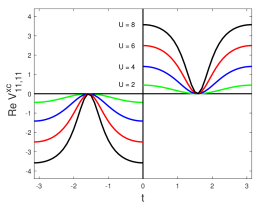
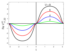
Figure 1: The real parts of the exchange-correlation potentials $V^{\mathrm{xc}}_{11,11}$ and $V^{\mathrm{xc}}_{11,22}$ of the Hubbard dimer as a function of time for $U=2,4,6,$ and $8$ with $\Delta=1$. Due to the particle-hole symmetry, $V_{\mathrm{xc}}(-t)=-V_{\mathrm{xc}}(t)$.

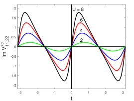
Figure 2: The imaginary parts of the exchange-correlation potentials $V^{\mathrm{xc}}_{11,11}$ and $V^{\mathrm{xc}}_{11,22}$ of the Hubbard dimer as a function of time for $U=2,4,6,$ and $8$ with $\Delta=1$. Due to the particle-hole symmetry, $V_{\mathrm{xc}}(-t)=-V_{\mathrm{xc}}(t)$.

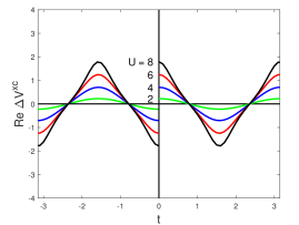
Figure 3: The real parts of the exchange-correlation potential in the bonding state $\phi_{\mathrm{B}}=\frac{1}{\sqrt{2}}(\varphi_{1}+\varphi_{2})$ and anti-bonding state $\phi_{\mathrm{A}}=\frac{1}{\sqrt{2}}(\varphi_{1}-\varphi_{2})$ as a function of time for $U=2,4,6,$ and $8$ with $\Delta=1$.

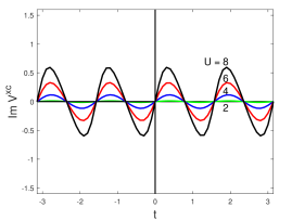
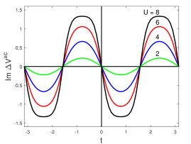
Figure 4: The imaginary parts of the exchange-correlation potential in the bonding and anti-bonding states as a function of time for $U=2,4,6,$ and $8$ with $\Delta=1$.

An interesting feature is the discontinuity of $V^{\mathrm{xc}}$ at $t=0$, which is the difference between the particle ($t=0^{+}$) and the hole ($t=0^{-}$) values, reminiscent of the discontinuity in the exchange-correlation potential in density functional theory perdew1982 .

One also notices that the time dependence is dictated by the excitation energies of the $(N\pm 1)$ systems and in general, these excitations include collective ones. For example, for solids one expects a time-dependent term of the form $\exp(-i\omega_{p}t)$ where $\omega_{p}$ is the plasmon energy. $V_{\mathrm{xc}}$ acts then as an effective external field, exchanging an energy $\omega_{p}$ with the system, as illustrated more explicitly later in the example on the Holstein Hamiltonian.

III.2 1D Hubbard chain

To calculate the Green function for the 1D Hubbard chain with the same Hamiltonian as in Eq. (28) but with $i,j=1,\dots,\infty$, the $V_{\mathrm{xc}}$ of the Hubbard dimer will be used as a model. This approximation neglects components of $V_{\mathrm{xc}}$ beyond nearest neighbors. Due to translational lattice symmetry it is convenient to introduce Bloch base functions,

$$\varphi_{k}(r)=\frac{1}{\sqrt{N}}\sum_{T}e^{ikT}\varphi(r-T),$$ (38)

where $T$ denotes a lattice site. The Green function expressed in these Bloch functions takes the form

$$G(r,r^{\prime};t)=\sum_{k}\varphi_{k}(r)G(k,t)\varphi_{k}^{\ast}(r^{\prime}),$$ (39)

where

$$G(k,t)=\int drdr^{\prime}\varphi_{k}^{\ast}(r)G(r,r^{\prime};t)\varphi_{k}(r^{\prime}).$$ (40)

The equation of motion in the Bloch base functions is given by

$$(i\partial_{t}-\varepsilon_{q})G(q,t)-F(q,t)=\delta(t),$$ (41)

where

$$\varepsilon_{q} =\int dr\varphi^{*}_{q}(r)h(r)\varphi_{q}(r)$$

$$=\frac{1}{N}\sum_{TT^{\prime}}e^{-ik(T-T^{\prime})}\varphi^{*}(r-T)h(r)\varphi(r-T^{\prime})$$

$$=-2\Delta\cos{q}$$ (42)

and

$$F(q,t)=\sum_{k}\int drdr^{\prime}$$

$$\times\varphi_{q}^{*}(r)\varphi_{k}(r)V_{\mathrm{xc}}(r,r^{\prime};t)\varphi_{k}^{*}(r^{\prime})\varphi_{q}(r^{\prime})\times G(k,t).$$ (43)

Since the Hartree potential is a constant it can be absorbed into the chemical potential.

To solve the equation of motion, one makes use of the $V^{\mathrm{xc}}$ deduced for the Hubbard dimer. The equations of motion of the Green function in the bonding and anti-bonding orbitals are given by

$$\left[i\partial_{t}-\varepsilon_{\mathrm{A}}-V^{\mathrm{xc}}(t)\right]G_{\mathrm{A}}(t)-\Delta V^{\mathrm{xc}}(t)G_{\mathrm{B}}(t)=\delta(t),$$ (44)

$$\left[i\partial_{t}-\varepsilon_{\mathrm{B}}-V^{\mathrm{xc}}(t)\right]G_{\mathrm{B}}(t)-\Delta V^{\mathrm{xc}}(t)G_{\mathrm{A}}(t)=\delta(t),$$ (45)

where

$$\varepsilon_{\mathrm{A}}=\Delta,\;\;\;\varepsilon_{\mathrm{B}}=-\Delta.$$ (46)

are the one-particle anti-bonding and bonding energies. $V^{\mathrm{xc}}$ and $\Delta V^{\mathrm{xc}}$ are given, respectively, in Eqs. (36) and (37).

With respect to the Hubbard chain, the bonding and anti-bonding states correspond to the centers of the occupied and unoccupied bands. A physically motivated approximation is to replace $G_{\mathrm{A}}(G_{\mathrm{B}})$ by $G(q,t)$ and $G_{\mathrm{B}}(G_{\mathrm{A}})$ by the average $\frac{1}{N}\sum_{k}G(k,t)$:

$$\left[i\partial_{t}-\varepsilon_{q}-V^{\mathrm{xc}}(t)\right]G(q,t)-\frac{1}{N}\sum_{k}\Delta V^{\mathrm{xc}}(t)G(k,t)=\delta(t).$$ (47)

One may rewrite the above equation as follows:

$$\left[i\partial_{t}-\varepsilon_{q}-V^{\mathrm{xc}}(t)-\Delta{V}^{\mathrm{xc}}(q,t)\right]G(q,t)=\delta(t),$$ (48)

where

$$\Delta{V}^{\mathrm{xc}}(q,t)=\frac{1}{N}\sum_{k}\Delta V^{\mathrm{xc}}(t)\frac{G(k,t)}{G(q,t)}.$$ (49)

The solution for the electron case is assumed to be given by

$$G^{e}(q,t)=-i\theta(t)e^{-i\varepsilon_{q}t-i\int_{0}^{t}dt^{\prime}\left[V^{\mathrm{xc}}(t^{\prime})+\Delta V^{\mathrm{xc}}(q,t^{\prime})\right]}.$$ (50)

A similar result can be readily derived for the hole Green function, keeping in mind that $V^{\mathrm{xc}}(-t)=-V^{\mathrm{xc}}(t)$.

To proceed further, the following approximation is proposed:

$$\Delta V^{\mathrm{xc}}(q,t)\approx\frac{1}{N}\sum_{k}\Delta V^{\mathrm{xc}}(t)e^{-i(\varepsilon_{k}-\varepsilon_{q})t},$$ (51)

which corresponds to replacing $G$ by the non-interacting $G^{0}$. Furthermore, to facilitate analytical calculations $V^{\mathrm{xc}}$ and $\Delta V^{\mathrm{xc}}$ in Eqs. (36) and (37) are expanded as follows:

$$V^{\mathrm{xc}}(t)\approx\frac{\alpha U}{2},$$ (52)

$$\Delta V^{\mathrm{xc}}(t)\approx\frac{\alpha U}{2}(1-\alpha^{2})e^{-i2\Delta t}.$$ (53)

In the above approximation the constant term that shifts the one-particle energy and the main excitation term $\exp{(-i2\Delta t)}$ that generates the main satellites are kept whereas the higher excitation term $\exp{(-i4\Delta t)}$ is neglected. One obtains to first order in $\Delta V^{\mathrm{xc}}$

$$G^{e}(q,t)=-i\theta(t)e^{-i(\varepsilon_{q}+\frac{\alpha U}{2})t}$$

$$\times\left\{1-i\frac{\alpha U}{2}(1-\alpha^{2})\frac{1}{N}\sum_{k}\int_{0}^{t}dt^{\prime}e^{-i(\varepsilon_{k}-\varepsilon_{q}+2\Delta)t^{\prime}}\right\}.$$ (54)

Performing the time integral one finds

$$G^{e}(q,t)=-i\theta(t)e^{-i(\varepsilon_{q}+\frac{\alpha U}{2})t}$$

$$\times\left\{1+\frac{\alpha U}{2}(1-\alpha^{2})\frac{1}{N}\sum_{k}\frac{e^{-i(\varepsilon_{k}-\varepsilon_{q}+2\Delta)t}-1}{\varepsilon_{k}-\varepsilon_{q}+2\Delta}\right\}.$$ (55)

Fourier transformation to the frequency domain yields

$$G^{e}(q,\omega) =\frac{A^{e}_{0}}{\omega-\left(\varepsilon_{q}+\frac{\alpha U}{2}\right)+i\eta}$$

$$+\frac{1}{N}\sum_{k}\frac{A^{e}(k)}{\omega-(\varepsilon_{k}+\frac{\alpha U}{2}+2\Delta)+i\eta},$$ (56)

where

$$A^{e}_{0}=1-\frac{\alpha U}{2}(1-\alpha^{2})\frac{1}{N}\sum_{k}\frac{1}{\varepsilon_{k}-\varepsilon_{q}+2\Delta},$$ (57)

$$A^{e}(k)=\frac{\alpha U}{2}(1-\alpha^{2})\frac{1}{\varepsilon_{k}-\varepsilon_{q}+2\Delta}.$$ (58)

A similar derivation can be carried out for the hole Green function and the result is given by

$$G^{h}(q,t)=i\theta(-t)e^{-i(\varepsilon_{q}-\frac{\alpha U}{2})t}$$

$$\times\left\{1-\frac{\alpha U}{2}(1-\alpha^{2})\frac{1}{N}\sum_{k}\frac{e^{-i(\varepsilon_{k}-\varepsilon_{q}-2\Delta)t}-1}{\varepsilon_{k}-\varepsilon_{q}-2\Delta}\right\},$$ (59)

$$G^{h}(q,\omega) =\frac{A^{h}_{0}}{\omega-\left(\varepsilon_{q}-\frac{\alpha U}{2}\right)-i\eta}$$

$$-\frac{1}{N}\sum_{k}\frac{A^{h}(k)}{\omega-(\varepsilon_{k}-\frac{\alpha U}{2}-2\Delta)-i\eta},$$ (60)

where

$$A^{h}_{0}=1+\frac{\alpha U}{2}(1-\alpha^{2})\frac{1}{N}\sum_{k}\frac{1}{\varepsilon_{k}-\varepsilon_{q}-2\Delta},$$ (61)

$$A^{h}(k)=\frac{\alpha U}{2}(1-\alpha^{2})\frac{1}{\varepsilon_{k}-\varepsilon_{q}-2\Delta}.$$ (62)

For the electron/hole case it is understood that both $\varepsilon_{k}$ and $\varepsilon_{q}$ correspond to unoccupied/occupied states.

Figure 5: The total spectral functions of the 1D Hubbard chain for $U=0,4,6,$ and $8$. A broadening of $0.1$ has been used.

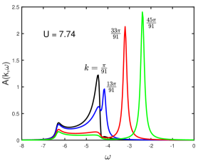
Figure 6: The $k$-resolved spectral functions of the 1D Hubbard chain for $U=7.74$. The $U$ and $k$ values have been chosen to facilitate comparison with Fig. 11 of Ref. benthien2007 . Within the approximation used, there is no spectral weight for $k=\frac{75\pi}{91}$ and $\frac{90\pi}{91}$ below the chemical potential, as explained in the text. A broadening of $0.1$ has been used.

Figure 7: The calculated band gap, $\alpha U$, compared with the exact gap obtained from the Bethe ansatz as a function of $U$. The calculated gap approaches the exact result as $U$ increases.

The calculated total spectral functions for $U=2,4,6,$ and $8$ are shown in Fig. 5 and the $k$-resolved spectra are illustrated in Fig. 6 for a few $k$-points corresponding to $U=7.74$. This value has been chosen in order to make comparison with the results obtained using the dynamical density-matrix renormalization group method benthien2007 . Due to the approximation made in replacing $G$ with $G^{0}$ in Eq. (49), there is no spectral weight below the chemical potential arising from the electron Green function and similarly, there is no spectral weight above the chemical potential arising from the hole Green function. For this reason, there is no spectral weight below the chemical potential for $k=\frac{75\pi}{91}$ and $k=\frac{90\pi}{91}$ when compared with the results shown in Fig. 11 of Benthien and Jeckelmann benthien2007 . Furthermore, the peaks are sharp $\delta$-functions but with some weight transferred to higher or lower energy. It is known that for a one-dimensional interacting system, a removal/addition of an electron results in two branches consisting of a spinless holon/antiholon dispersion with a hole/electron charge and a charge-neutral spinon dispersion of spin $\frac{1}{2}$.

Although the approximation used is very simple, the $k$-resolved spectra shown in Fig. 6 is in favorable agreement with those calculated using the dynamical density-matrix renormalization group method benthien2007 . A notable discrepancy is the dispersion widths for both the spinon and the holon branches. Thus, the peak positions at small $k$ are lower in energy compared with those in Ref. benthien2007 . This is understandable since within the approximation used, the dispersion is pinned down by the non-interacting $G^{0}$ and the use of the Hubbard dimer $V^{\mathrm{xc}}$ neglects long-range correlations, which tend to narrow the band dispersion.

The structure of the calculated $k$-resolved hole spectra in Fig. 6 can be understood from the explicit expression for the hole Green function in Eq. (60). The imaginary part of the first term is the main peak centered at $\omega=\varepsilon_{q}-\frac{\alpha U}{2}$, which is interpreted as the spinon excitation. The imaginary part of the second term with the weight $A^{h}(k)$ set to unity is the non-interacting occupied density of states shifted by $-(\frac{\alpha U}{2}+2\Delta)$. For $q=\frac{45\pi}{91}$ (green curve), the one-particle energy, $\varepsilon_{q}$, is approximately zero and the main peak is located at the top of the band edge at $\omega=-\frac{\alpha U}{2}$. The remaining spectra stretching approximately from $-6.5$ to $-4.5$ is the shifted occupied density of states weighted by $A^{h}(k)$. The peak feature at the lower edge at $-6.5$ reflects the same feature present in the shifted non-interacting occupied density of states ($U=0$ in Fig. 5) and may be interpreted as the holon excitation. The structure at the upper edge at around $-4.5$, on the other hand, arises from the enhanced weight of $A^{h}(k)$ which is largest for $q$ around the bottom of the non-interacting band, giving rise to a step-like structure benthien2007 . For $q=\frac{\pi}{91}$ (black curve), the main peak is centered at $\omega=-\frac{\alpha U}{2}-2\Delta$ and it merges with the shifted density of states. For $q=\frac{13\pi}{91}$ the main peak still lies outside the shifted density of states and a three-peak structure is then observed, as also found in the calculated spectra using the dynamical density-matrix renormalization group method benthien2007 . It is not immediately evident from the expressions for the Green function is Eqs. (56) and (59) how to interpret the two branches as spinon and holon excitations. Such interpretation would probably require analysis in terms of state vectors.

The calculated band gap, which is given by $\alpha U$, is displayed in Fig. 7 and compared with the exact result ovchinnikov1970 ,

$$E_{\mathrm{gap}}=\frac{16\Delta^{2}}{U}\int_{1}^{\infty}dy\frac{\sqrt{y^{2}-1}}{\sinh{\left(\frac{2\pi\Delta y}{U}\right)}},$$ (63)

obtained from the Bethe ansatz. The agreement between the analytically calculated gap and the exact gap is very close, despite the simplicity of the approximation. The calculated gap approaches the exact gap in the limit of large $U$ and a gap opens as soon as $U$ is finite, as in the exact case. The discrepancy is largest at small values of $U$, which may be understood from the lack of long-range screening effects in $V^{\mathrm{xc}}$ of the Hubbard dimer. It should be noted that in the widely used dynamical mean-field theory (DMFT) georges1996 within the single-site approximation, the gap is not opened up until $U>6$. Only within the cluster DMFT with an even number of sites does the gap form for any finite $U$ whereas with an odd number of sites a metallic region remains until $U$ exceeds a certain value before entering the Mott insulating phase through a coexistence region go2009 .

III.3 Holstein Hamiltonian

A simplified Holstein Hamiltonian describing a coupling between a core electron and a set of bosons, such as plasmons or phonons, is given by langreth1970

$$\hat{H}=\varepsilon\hat{c}^{\dagger}\hat{c}+\sum_{q}\hat{c}\hat{c}^{\dagger}g_{q}(\hat{b}_{q}+\hat{b}_{q}^{\dagger})+\sum_{q}\omega_{q}\hat{b}_{q}^{\dagger}\hat{b}_{q},$$ (64)

where $\varepsilon$ is the core electron energy, $\omega_{q}$ is the boson energy of wave vector $q$, and $\hat{c}$ and $\hat{b}_{q}$ are respectively the core electron and the boson operators. This Hamiltonian can be solved analytically and the algebra is simplified if it is assumed that the boson is dispersionless with an average energy $\omega_{p}$. Under this assumption, the exact solution for the core-electron removal spectra yields langreth1970

$$A(\omega)=\sum_{n=0}^{\infty}f_{n}\delta(\omega-\varepsilon-\Delta\varepsilon+n\omega_{p}),$$ (65)

where

$$f_{n}=\frac{e^{-a}a^{n}}{n!},\;\;a=\sum_{q}\left(\frac{g_{q}}{\omega_{p}}\right)^{2},\;\;\Delta\varepsilon=a\omega_{p}.$$ (66)

This exact solution can also be obtained using the cumulant expansion bergersen1973 ; hedin1980 ; almbladh1983 . The hole Green function corresponding to the above spectra is given by

$$G(t<0)=i\sum_{n=0}^{\infty}f_{n}e^{-i(\varepsilon+\Delta\varepsilon-n\omega_{p})t}\theta(-t).$$ (67)

It can be verified that the time-dependent exchange-correlation potential corresponding to the Holstein Hamiltonian reads

$$V_{\mathrm{xc}}(t<0)=\Delta\varepsilon\left(1-e^{i\omega_{p}t}\right).$$ (68)

This expression provides a very simple interpretation: the first term corrects the non-interacting core-electron energy whereas the second term describes the bosonic mode interacting with the core electron, which can exchange not only one but multiple quanta of $\omega_{p}$ with the field. This is precisely what is accomplished by the cumulant expansion bergersen1973 ; hedin1980 ; almbladh1983 within the self-energy formulation but in an ad hoc and complicated manner.

III.4 Hydrogen atom

It may seem trivial to consider the hydrogen atom since it is not a many-electron system. Nevertheless, it illustrates a number of exact results such as the sum rule in Eq. (10) and the condition in Eq. (11). For the hydrogen atom, the hole Green function is given by

$$G(r,r^{\prime};t<0)=i\varphi_{s}(r)\varphi_{s}(r^{\prime})\exp(-i\varepsilon_{s}t)\theta(-t),$$ (69)

where $\varphi_{s}$ and $\varepsilon_{s}$ are the $1s$-orbital and its energy. The exchange-correlation potential for $t<0$ can be readily deduced yielding

$$V_{\mathrm{xc}}(r,r^{\prime};t<0)=-V_{\mathrm{H}}(r)=-\int dr^{\prime\prime}v(r-r^{\prime\prime})|\varphi_{s}(r^{\prime\prime})|^{2},$$ (70)

independent of $r^{\prime}$ and $t$, cancelling the spurious Hartree potential. The corresponding exchange-correlation hole is then given by

$$\rho_{\mathrm{xc}}(r,r^{\prime},r^{\prime\prime};t<0)=-|\varphi_{s}(r^{\prime\prime})|^{2}.$$ (71)

It can also be seen that the condition in Eq. (11),

$$\rho_{\mathrm{xc}}(r,r^{\prime},r;t<0)=-\rho(r),$$ (72)

as well as the sum rule in Eq. (10),

$$\int dr^{\prime\prime}\rho_{\mathrm{xc}}(r,r^{\prime},r^{\prime\prime};t<0)=-\int dr^{\prime\prime}|\varphi_{s}(r^{\prime\prime})|^{2}=-1,$$ (73)

are both fulfilled, as they should be.

IV Conclusion

The exchange-correlation formalism has been applied to determine the Green function of the 1D Hubbard chain by utilizing the exchange-correlation potential derived from the Hubbard dimer. Under the approximation corresponding to replacing the full Green function by a non-interacting Green function in the first iteration, the spectral functions can be calculated analytically. Despite the very simple approximation, the results compare favorably with the more accurate results calculated using the dynamical density-matrix renormalization group method. Peak structures corresponding to the holon and spinon collective excitations are correctly reproduced, although the positions are too low for small $k$, due to the use of a non-interacting Green function and the neglect of long-range correlations in the exchange-correlation potential of the Hubbard dimer. The calculated gap agrees very well with the exact result obtained from the Bethe ansatz. These very encouraging results may indicate the robustness of the exchange-correlation potential, insensitive to the system size, allowing for extrapolation from a small to a large system. By using the exact $V^{\mathrm{xc}}$ of the Hubbard dimer, it is ensured that the sum-rule is fulfilled.

An example from the Holstein Hamiltonian further illustrates the potential of the exchange-correlation formalism. The exact $V^{\mathrm{xc}}$ has a very simple form, offering a clear physical interpretation. The main collective charge excitation (plasmon) determines the characteristic energy of the time-dependent part of $V^{\mathrm{xc}}$ while the constant term provides a correction to the one-particle energy. One may speculate that a generic structure of the exchange-correlation potential consists of a constant term and a series of time-dependent terms of exponential form with energies characteristic of the excitations of the $(N\pm 1)$-systems.

An example of the hydrogen atom illustrates the exact properties of the exchange-correlation hole.

References

• (1) F. Aryasetiawan, Phys. Rev. B 105, 075106 (2022).
• (2) T. Giamarchi, Quantum Physics in One Dimension (Clarendon Press, Oxford, 2004).
• (3) F. H. L. Essler, H. Frahm, F. GΓΆhmann, A. KlΓΌmper, and V. E. Korepin, The One-Dimensional Hubbard Model (Cambridge University Press, Cambridge, 2005).
• (4) H. Benthien and E. Jeckelmann, Phys. Rev. B 75, 205128 (2007).
• (5) S. Sorella and A. Parola, J. Phys.: Condens. Matter 4, 3589 (1992).
• (6) K. Penc, K. Hallberg, F. Mila, and H. Shiba, Phys. Rev. Lett. 77, 1390 (1996).
• (7) V. Meden and K. SchΓΆnhammer, Phys. Rev. B 46, 15753 (1992).
• (8) J. Voit, Phys. Rev. B 47, 6740 (1993).
• (9) C. Kim, A. Y. Matsuura, Z.-X. Shen, N. Motoyama, H. Eisaki, S. Uchida, T. Tohyama, and S. Maekawa, Phys. Rev. Lett. 77, 4054 (1996).
• (10) C. Kim, Z.-X. Shen, N. Motoyama, H. Eisaki, S. Uchida, T. Tohyama, and S. Maekawa, Phys. Rev. B 56, 15589 (1997).
• (11) See, for example, A. L Fetter and J. D Walecka, Quantum Theory of Many-Particle Systems, (Dover, Mineola, New York, 2003).
• (12) A. D. Becke, J. Chem. Phys. 140, 18A301 (2014).
• (13) J. C. Slater, Phys. Rev. 81, 385 (1951).
• (14) J. C. Slater, Phys. Rev. 165, 658 (1968).
• (15) L. Hedin, Phys. Rev. 139, A796 (1965).
• (16) F. Aryasetiawan and O. Gunnarsson, Rep. Prog. Phys. 61, 237 (1998).
• (17) W. Kohn and L. J. Sham, Phys. Rev. 140, A1133 (1965).
• (18) B. D. E. McNiven, G. T. Andrews, J. P. F. LeBlanc, Phys. Rev. B 104, 125114 (2021).
• (19) O. Gunnarsson and B. I. Lundqvist, Phys. Rev. B 13, 4274 (1976).
• (20) R. O. Jones and O. Gunnarsson, Rev. Mod. Phys. 61, 689 (1989).
• (21) J. P. Perdew, R. G. Parr, M. Levy, and J. L. Balduz, Phys. Rev. Lett. 49, 1691 (1982).
• (22) A. A. Ovchinnikov, Sov. Phys. JETP 30, 1160 (1970).
• (23) A. Georges, G. Kotliar, W. Krauth, and M. J. Rozenberg, Rev. Mod. Phys. 68, 13 (1996).
• (24) A. Go and G. S. Jeon, J. Phys.: Condens. Matter 21, 485602 (2009).
• (25) D. C. Langreth, Phys. Rev. B 1, 471 (1970).
• (26) B. Bergersen, F. W. Klus, and C. Blomberg, Can. J. Phys. 51, 102 (1973).
• (27) L. Hedin, Phys. Scr. 21, 477 (1980).
• (28) C.-O. Almbladh and L. Hedin, in Handbook on Synchroton Radiation, edited by E. E. Koch (North-Holland, Amsterdam, 1983) Vol. 1, p.686.