The pion in the graviton soft-wall model: phenomenological applications

Abstract

The holographic graviton soft-wall model, introduced to describe the spectrum of scalar and tensor glueballs, is improved to incorporate the realization of chiral-symmetry as in QCD. Such a goal is achieved by including the longitudinal dynamics of QCD into the scheme. Using the relation between AdS/QCD and Light-Front dynamics, we construct the appropriate wave function for the pion which is used to calculate several pion observables. The comparison of our results with phenomenology is remarkably successful.

1 Introduction

In the last few years, hadronic models, inspired by the holographic conjecture [1, 2], have been vastly used and developed in order to investigate non-perturbative features of glueballs and mesons, thus trying to grasp fundamental features of QCD [3, 4]. Recently we have used the so called AdS/QCD models to study the meson and glueball spectrum spectrum [5, 6, 7, 8]. The holographic principle relies in a correspondence between a five dimensional classical theory with an AdS metric and a supersymmetric conformal quantum field theory with $N_{C}\rightarrow\infty$. This theory, different from QCD, is taken as a starting point to construct a 5 dimensional holographic dual of it. This is the so called bottom-up approach  [9, 10, 11, 12, 13]. The relation of this approach established with QCD is at the level of the leading order in the number of colors expansion.

In our previous investigation, we could successfully describe the pseudo-scalar spectrum, identified with the $\eta$ system, without any free parameter [8] within the GSW model. However, we found that the conventional model was not able to distinguish between the spectrum of the $\eta$ and the $\pi$ [8]. One of the differences between the $\eta$ and the $\pi$ is the isospin, however since the GSW does not take into account Coulomb corrections, the pions behave very much like the $\eta$ from the point of view of quantum numbers and therefore the spectrum would be the same, but certainly not in nature. In order to characterize the pion we proposed at that time a modification of the dilaton in analogy with previous investigations [13, 14, 15]. Such a procedure was able to describe correctly the pion spectrum, however we found out that the wave function derivable from the mode function was not precise enough to explain many of the data that follow. Other authors have also studied chiral symmetry breaking within holographic models in the Hard Wall approach in an aim to match the high and the low energy behavior or QCD [16, 11, 17, 18].

In here we will proceed in a way which follows closer QCD by matching our AdS/QCD model with Light Front holography. The pion is the Goldstone boson of SU(2) x SU(2) chiral symmetry and this fact is instrumental in giving the lightest pion its low mass. We should therefore implement the spontaneous broken realization of chiral symmetry in the GSW holographic model to reproduce the low mass of the ground state of the pion. To do so we will modify the dilaton of the GSW model to get a zero mass pion. To implement chiral symmetry breaking we will include the QCD longitudinal dynamics [19, 20, 21, 22, 23]. In this way we will obtain a pion at the physical mass. We also obtain the corresponding mode function.

In order to establish to what extent the mechanism is phenomenologically successful, we calculate several pion observables comparing the outcomes with data. To this aim, a correspondence between the mode function and a light cone wave functions is introduced [24, 25, 26]. The comparison between our calculations and the phenomenological results is quite reasonable despite the low number of parameters.

The contents of this presentation go as follows. In Section 2 we describe the $\eta$ Equation of Motion (EoM) of the GSW model and its solution. We proceed in Section 3 to show the description of the Goldstone pion in the GSW model. In Section 4 we establish the relation between the pion mode function and the pion light cone wave function (wf). In order to effectively describe the chiral symmetry breaking, the longitudinal dynamics is introduced in Section 5. Having completed the description of the pion model, in Section 6 we calculate various pion observables: the spectrum, the form factor, the mean square radius, the effective form factor, the mean transverse distance between two partons, the decay constant, the distribution amplitude, the photon transition form factor and the parton distribution function (PDF). Results are compared with the phenomenology. We end by some concluding remarks.

2 The pseudo-scalar wave equation within the GSW model

In this section, details on the application of the GSW model to the study of the pseudo-scalar meson spectrum are presented. Our approach is based on the usual Soft Wall (SW) AdS/QCD model [26, 12] modified by a deformation of the $AdS_{5}$ space. These type of changes have been proposed in several analyses to improve the prediction power of the holographic models within the bottom-up framework  [27, 28, 29, 30, 31]. In particular, the GSW model has been specifically introduced to describe the scalar and tensor glueball spectrum [5]. Previously it was shown that the conventional field approach was hardly capable to describe the glueball spectra [28, 32]. Therefore, in Ref. [5] the glueball masses have been calculated from the mode function of gravitons propagating on a deformed $AdS_{5}$ space. The wrap metric of the model effectively encodes complex dilatonic effects. In particular the metric used was

$$ds^{2}=\frac{R^{2}}{z^{2}}e^{\alpha k^{2}z^{2}}(dz^{2}+\eta_{\mu\nu}dx^{\mu}dx^{\nu})=e^{\alpha{k^{2}z^{2}}}g_{MN}dx^{M}dx^{N}=\bar{g}_{MN}dx^{M}dx^{N}.$$ (1)

Recently, in Refs. [6, 7, 8] the GSW has been applied to describe also the spectrum of various mesons and high spin glueballs. The parameters entering the GSW model are $\alpha=0.55\pm 0.04$ and the energy scale $k=0.37/\sqrt{\alpha}$ GeV. Within these values the model is able to reproduce quite accurately the meson and glueball spectra, except for the pion which requires proper modifications to include the chiral symmetry breaking mechanism [8]. In this case however, the pion spectrum comes out close to the experimental data although the calculation predicts the existence of up to now not found additional states.

Let us proceed now to build up the model for the pion, which is closer to the phenomenology than that of Ref. [8]. We start from the pseudo-scalar action,

$$S=\int d^{5}x~{}e^{-\varphi_{0}(z)}\sqrt{-g}\Big{[}g^{MN}\partial_{M}\Phi(x)\partial_{N}\Phi(x)-4e^{\alpha k^{2}z^{2}}\Phi(x)^{2}\Big{]}~{},$$ (2)

where $\varphi_{0}(z)=k^{2}z^{2}$ and we have explicitly used the five dimensional pseudo-scalar mass $M_{5}R^{2}=-4$ [33]. The EoM for the pseudo-scalar system can be recast in a Schrödinger type equation by scaling the field,

$$\Phi(x,z)=e^{iP\cdot x}e^{\varphi_{0}(z)/2}\chi(z)z^{3/2},$$ (3)

where $P^{2}=M^{2}$, $M$ being the mass of the pseudo-scalar meson. The final equation has the form

$$-\frac{d^{2}\chi(z)}{dz^{2}}+V(z)\chi(z)=M^{2}\chi(z).$$ (4)

where the potential is

$$V(z)=k^{4}z^{2}+2k^{2}+\frac{15}{4z^{2}}-\frac{4}{z^{2}}e^{\alpha k^{2}z^{2}}.$$ (5)

However, since the potential Eq.(5) is not binding, an additional dilaton $\varphi_{n}(z)$ has been added to the action Eq. (2) so that the exponential $exp[\alpha k^{2}z^{2}]$ in Eq. (5) can be truncated so that the final potential binds. Details on this procedure have been described in detail in Ref. [8]. The Schrödinger equation is now obtained by imposing the following re-scale:

$$\Phi(x,z)=e^{iP\cdot x}e^{(\varphi_{0}(z)+\varphi_{n}(z))/2}~{}\chi(z)z^{3/2},$$ (6)

then, the truncated phenomenological potential becomes:

$$V(z)=k^{4}z^{2}(1-2\alpha^{2})+2k^{2}(1-2\alpha)-\frac{1}{4z^{2}}$$ (7)

The regular solution to the above differential equation, for the $n$th mode is,

$$\chi_{n}(z) =N_{n}z^{\frac{1}{2}}e^{-\frac{\sqrt{1-2\alpha^{2}}}{2}k^{2}z^{2}}~{}_{1}F_{1}\left(-n,1,\sqrt{1-2\alpha^{2}}k^{2}z^{2}\right)~{},$$ (8)

where $N_{n}$ is a normalization constant and the pseudo-scalar mass comes out,

$$M(n)^{2}=\Big{[}(2-4\alpha)+2\sqrt{1-2\alpha^{2}}(1+2n)\Big{]}k^{2}.$$ (9)

It is immediate that, $M(0)\neq 0$, a consequence of the fact that the model does not incorporate chiral symmetry. We identify this state with the dual of $\eta$ meson. The spectrum, shown in Ref. [8] is in good agreement with data.

3 The pion in the GSW model

In QCD if the quark masses are zero, chiral symmetry is spontaneously broken and the pion is the corresponding Goldstone boson. Therefore if we want an AdS/QCD model which represents this QCD behaviour we have to obtain an EoM for a massless pion. In this holographic framework the dilaton must describe much the essence of the confinement mechanism together with the chiral symmetry breaking. Therefore, our formalism, connecting the pseudo-scalar spectrum to that of the $\eta$, requires a modification of the dilaton to generate the exact chiral limit. From a phenomenological point of view, it is necessary to get a massless pion and an energy scale bigger then that of the $\eta$, as signaled by pion mass hierarchy. For this purpose, we propose a straightforward modification of the additional dilaton $\varphi_{n}(z)$ used for the $\eta$ [8]. It will be sufficient to introduce two additional constants in the cut off potential. Therefore, for the pion within the GSW model we propose the following action:

$$S=\int d^{5}x~{}e^{-\varphi_{0}(z)-\varphi_{n}(z)}\sqrt{-g}\Big{[}g^{MN}\partial_{M}\Phi(x)\partial_{N}\Phi(x)-4e^{\alpha k^{2}z^{2}}\Phi(x)^{2}\Big{]}.$$ (10)

If the additional dilaton satisfies the following differential equation (see Ref. [8] for details):

$$-\frac{\varphi_{n}^{{}^{\prime\prime}}(z)}{2}+\varphi_{n}^{{}^{\prime}}(z)\left(\frac{3}{2z}+k^{2}z\right)+\frac{\varphi_{n}^{{}^{\prime}}(z)^{2}}{4}-\frac{4}{z^{2}}\left[e^{\alpha k^{2}z^{2}}-1-(\alpha+\xi_{\pi})k^{2}z^{2}-\frac{1}{2}(\alpha^{2}+\gamma_{\pi})k^{4}z^{4}\right]=0~{},$$ (11)

where the parameters $\xi_{\pi}$ and $\gamma_{\pi}$ have been included at variance of the $\eta$ case [8]. The relative potential in the Schrödinger representation will be:

$$V_{\pi}(z)=\frac{15}{4z^{2}}+2k^{2}+k^{4}z^{2}-\frac{4}{z^{2}}\left[1+(\alpha+\xi_{\pi})k^{2}z^{2}+\frac{1}{2}(\alpha^{2}+\gamma_{\pi})k^{4}z^{4}\right]=V_{\eta}(z)-4k^{2}\xi_{\pi}-2\gamma_{\pi}k^{4}z^{2}~{}.$$ (12)

For this potential the mass equation becomes

$$M_{\pi}^{2}(n)=\big{[}2-4(\alpha+\xi_{\pi})+2\sqrt{1-2(\alpha^{2}+\gamma_{\pi})}(1+2n)\big{]}k^{2}.$$ (13)

If one imposes $M_{\pi}(0)=0$ then:

$$\xi_{\pi}=\dfrac{1-2\alpha+\sqrt{1-2\alpha^{2}-2\gamma_{\pi}}}{2}.$$ (14)

This relation ensures that the lightest pion is a Goldstone boson. The mass spectrum then becomes

$$M^{2}_{\pi}(n)=4\sqrt{1-2(\alpha^{2}+\gamma_{\pi})}~{}k^{2}n~{}.$$ (15)

Thus, the parameter $\gamma_{\pi}$ modifies the $\eta$ slope of the spectrum to reproduce the pion excitations. This freedom relaxes the energy scale from the GSW scale $\sqrt{\alpha}k$. The $n$th solution to the relative Schrödinger equation is:

$$\chi_{n}(z) =N_{n}z^{\frac{1}{2}}~{}exp\left(-\frac{\sqrt{(1-2(\alpha^{2}-\gamma_{\pi})}}{2}k^{2}z^{2}\right)~{}_{1}F_{1}\left(-n,1,\sqrt{(1-2(\alpha^{2}+\gamma_{\pi})}k^{2}z^{2}\right)~{}.$$ (16)

where the difference with respect to Eq.(8) is characterized by the presence of $\gamma_{\pi}$.

A caveat is in place. The experimental status for the pion excitations is not well established and therefore possible intermediate states between $\pi$, $\pi^{\prime}$ and $\pi^{\prime\prime}$ could be observed in the future as discussed in Ref. [8]. However, if one tries to describe the present experimental spectrum as described in Ref. [34, 35], different energy scales for the scalar, the $\eta$ and the pion spectra are necessary. The modification proposed here preserves entirely the GSW description of the pseudo-scalar structure but incorporates a new scale and a massless pion ground state. In the future other different possibilities will be investigated. In the present study we mainly focus on this strategy which preserves as much as possible the GSW structure of the model. In the next sections phenomenological predictions and comparisons with observable will be provided.

4 Pseudo-scalar Light Front wave function

In order to test the proposed approach, let us take advantage of the correspondence between the AdS/QCD approach and the Light-Front formalism that characterizes the non perturbative structure of hadrons [24, 36]. Such a strategy is fundamental to use the AdS/QCD model to evaluate other observables and learn new information on the inner structure of the hadrons. Here we recall how to translate the mode function derived from the AdS EoM, e.g. from Eq. (16) for the pion, in terms of the corresponding Light-Front (LF) wave function [25, 37, 38]. This procedure is extremely convenient for calculating observables to test the proposed models. In particular, we follow the formalism presented in Ref. [26] where such a procedure has been applied to the hard-wall (HW) and SW models in order to describe the pion and the bulk-to-boundary propagator (the dual to the electromagnetic conserved current).

4.1 The light front formalism

Let us first recall the main essence of the LF Fock representation of hadronic systems. As shown in Ref.  [24] the QCD quantization at fixed LF time $\tau=t+x_{3}/c$ allows to describe the hadron spectrum from a Lorentz-invariant hamiltonian: $\hat{H}_{LFQCD}=P^{-}P^{+}-\mathbf{P}_{\perp}^{2}$, where the hadron four momentum, described with LF coordinates, has been introduced: $P^{\mu}=(P^{+},P^{-},\mathbf{P}_{\perp})$ and $P^{\pm}=P_{0}\pm P^{3}$. The plus and transverse components are kinematical operators. $P^{-}=id/d\tau$ is responsible for the LF time evolution of the system. The mass equation can be then introduced as

$$\hat{H}_{LFQCD}|\psi_{h}\rangle=M^{2}_{h}|\psi_{h}\rangle~{},$$ (17)

where $|\psi_{h}\rangle$ represents the hadron state. Remarkably, the LF quantization, if the $A^{+}=0$ gauge is considered, leads to a suppression of all intermediate gluon degrees of freedom justifying a Fock expansion of the hadron state in terms of free partons. Therefore:

$$|\psi_{h}(P^{+},\mathbf{P}_{\perp},S_{z})\rangle =\sum_{n,\lambda_{i}}\prod_{i=1}^{n}\int\dfrac{dx_{i}d^{2}\mathbf{k}_{\perp i}}{2\sqrt{x_{i}}(2\pi)^{3}}(16\pi)^{3}\delta\left(1-\sum_{j=1}^{n}x_{j}\right)\delta^{(2)}\left(\sum_{j=1}^{n}\mathbf{k}_{\perp i}\right)$$ (18)

$$=\psi_{n/h}(x_{i},\mathbf{k}_{\perp i},\lambda_{i})|x_{i}P^{+},x_{i}\mathbf{{P}_{\perp}}+\mathbf{k}_{\perp i},\lambda_{i}\rangle_{n};$$

where here $\mathbf{k}_{\perp i}$ is the intrinsic transverse momentum of the $i$ parton, $\lambda_{i}$ is the helicity, $n$ the number of Fock states taken in the sum, e.g. for mesons $n\geq 2$. $\psi_{n/h}$ is the frame independent LF wf which incorporates the probability that the hadronic system can be described by $n$ constituents. $|k^{+}_{i},\mathbf{K}_{\perp i},\lambda_{i}\rangle_{n}$ represents the Fock state of $n$ free partons, which is an eigenstate of the free LF Hamiltonian. The normalization condition reads,

$$\langle\psi_{h}(P^{+},\mathbf{P}_{\perp},S_{z})|\psi_{h}(P^{\prime+},\mathbf{P^{\prime}}_{\perp},S^{\prime}_{z})\rangle=2P^{+}(2\pi)^{3}\delta_{S_{z}~{}S^{\prime}_{z}}\delta(P^{+}-P^{\prime+})\delta^{(2)}(\mathbf{P}_{\perp}-\mathbf{P^{\prime}}_{\perp}),$$ (19)

and leads to,

$$\sum_{n=2}^{\infty}\prod_{i=1}^{n}\int\dfrac{dx_{i}\mathbf{k}_{\perp i}}{2(2\pi)^{3}}(16\pi^{3})\delta\left(1-\sum_{j=1}^{n}x_{j}\right)\delta^{(2)}\left(\sum_{j=1}^{n}\mathbf{k}_{\perp i}\right)|\psi_{n/h}(x_{i},\mathbf{k}_{\perp i})|^{2}=1~{}.$$ (20)

Since in the present analysis we shall not investigate polarization effects, i.e. we will evaluate unpolarized distributions, we omit here the helicity dependence. Moreover, the AdS mode functions are obtained in terms of the coordinates of a $5$-dimensional space, therefore it is useful to rewrite the above condition in terms of $\tilde{\psi}_{n/h}(x_{i},\mathbf{b}_{\perp i})$, i.e. the Fourier Transform (FT) of $\psi_{n/h}(x_{i},\mathbf{k}_{\perp i})$, which results in

$$\psi_{n/h}(x_{j},\mathbf{k}_{\perp j})=(4\pi)^{(n-1)/2}\prod_{i=1}^{n-1}d^{2}\mathbf{b}_{\perp i}exp{\left(\displaystyle i\sum_{u=1}^{n-1}\mathbf{b}_{\perp i}\cdot\mathbf{k}_{\perp i}\right)}\tilde{\psi}_{n/h}(x_{i},\mathbf{b}_{\perp i})~{},$$ (21)

where $\mathbf{b}_{\perp i}$ is the conjugate variable to $\mathbf{k}_{\perp i}$ and represents the frame independent intrinsic coordinate. The normalization for the LF wf in coordinate space reads,

$$\sum_{n=2}^{\infty}\prod_{i=1}^{n}\int dx_{i}d^{2}\mathbf{b}_{\perp i}|\tilde{\psi}_{n/h}(x_{i},\mathbf{b}_{\perp i})|^{2}=1~{}.$$ (22)

4.2 The pion LF wave function

The procedure to relate the mode functions and the LF wf can obtained by comparing the Drell-Yan-West form factor [39] with the AdS one, see Ref. [26]. The AdS ff can be written from the overlap of the normalizable modes of the outgoing and incoming hadrons, $\Phi_{out}(z)$ and $\Phi_{in}(z)$ with the mode dual to the external electromagnetic source $J(Q^{2},z)$,

$$F(Q^{2})=\int\frac{dz}{z^{3}}~{}e^{-\varphi_{0}(z)-\varphi_{n}(z)}\Phi_{out}(z)J(Q^{2},z)\Phi_{in}(z),$$ (23)

where $J(Q^{2},z)$ is the bulk-to-boundary propagator. As it will be also discussed in the form factor section of this study, the Green’s function of a vector field equation, which has $M_{5}^{2}=0$, is the same for the GSW model as for the SW one [26] as shown in Refs. [29, 8]. Moreover, for large momenta the SW result coincides with that obtained within the HW model, and therefore we can apply the relation obtained in Ref. [26]. This last statement is because for large momenta the two form factors coincide since the dilaton dependence dies out.

To establish the connection between the two form factors, the mode-function, solution of the Schrödinger equation, is normalized as follows:

$$\int dz~{}\chi(z)^{2}=1~{}.$$ (24)

Moreover from Eq. (23) one gets the normalization of the mode function:

$$\int dz~{}\dfrac{e^{-\varphi_{0}(z)-\varphi_{n}(z)}}{z^{3}}\Phi(z)^{2}=1~{}.$$ (25)

The “density”distribution for the pion can be obtained from the mode functions and is related to the FT of the pion form factor [26],

$$\tilde{\rho}(x,z)=\dfrac{e^{-\varphi_{0}(z)-\varphi_{n}(z)}}{2\pi}\dfrac{x}{1-x}\dfrac{|\Phi(z)|^{2}}{z^{4}}=\dfrac{x}{1-x}\dfrac{|\chi(z)|^{2}}{2\pi z}=\dfrac{|\tilde{\psi}_{LF}(x,\vec{b}_{\perp})|^{2}}{(1-x)^{2}}~{},$$ (26)

where in the intermediate step use has been made of Eq. (6) for $z$ dependence. Furthermore, $x$ represents the longitudinal momentum fraction carried by a parton in the pion and $\mathbf{b}_{\perp}$ represents the transverse distance between the quark and the anti-quark. Finally, the relation between the pion LF wf and the mode function becomes:

$$\tilde{\psi}_{LF}(x,\mathbf{b}_{\perp})\equiv\tilde{\psi}_{2/\pi}(x,\mathbf{b}_{\perp})=\sqrt{\dfrac{x(1-x)}{2\pi z}}\chi(z)~{},$$ (27)

where $z=\sqrt{x(1-x)}|\mathbf{b}_{\perp}|$ [26]. This equation allows us to obtain the LF wf from the solution of our mode equation, namely the Schrödinger equation associated to potential $V_{\pi}(z)$ which appears in Eq.(12).

5 The longitudinal dynamics

A promising procedure to incorporate the chiral symmetry breaking in those models that have zero mass ground state pions, like that developed in Section 3, is to include longitudinal dynamics  [19, 20, 21, 22, 23]. To this aim we incorporate in our scheme the procedure developed in Ref. [22] and also applied to the SW model of Ref. [26]. In the LF AdS/QCD framework, the QCD hamiltonian for the pion is effectively described by equations such as Eqs.(7) and (12), which depend only on the transverse coordinates $\mathbf{z}=\sqrt{x(1-x)}\mathbf{b}_{\perp}$,

$$-\frac{d^{2}}{dz^{2}}+V_{\perp}(z)\phi(z)=M^{2}_{\perp}\phi(z)~{}.$$ (28)

Now we specify the perpendicular index, since the solution to the above equation represents the underlying transverse dynamics of the meson. However, the full description of pion structure and its spectroscopy requires an effective way to include the chiral symmetry breaking mechanism. To this aim we include longitudinal degrees of freedom in the GSW model, by following the line of thought of Ref. [22]. Such a goal can be reached by assuming that the full potential is a combination of two potentials, a transverse and a longitudinal, $V_{eff}=V_{\perp}+V_{||}$, and therefore the spectrum is given by two contributions to the mass $M_{\pi}^{2}=M^{2}_{\perp}+M_{||}^{2}$, determined by the equation,

$$\left[-\dfrac{d^{2}}{dz^{2}}+\dfrac{m_{q}^{2}}{x}+\dfrac{m_{\bar{q}}^{2}}{1-x}+V_{eff}\right]\bar{\Phi}(z,x)=M^{2}\bar{\Phi}(x,z)~{}.$$ (29)

The transverse quantities can be evaluated from holographic models, and the longitudinal wf, and its corresponding spectrum component, can be obtained from the Schrödinger equation,

$$\left[\dfrac{m_{q}^{2}}{x}+\dfrac{m_{\bar{q}}^{2}}{1-x}+V_{||}(x)\right]\Xi(x) =M^{2}_{||}~{}\Xi(x)~{},$$ (30)

where he $\Xi(x)$ is the longitudinal wf. In this approach the overall wf is given by

$$\bar{\Phi}(x,\mathbf{b}_{\perp})=\tilde{\psi}_{LF}(x,\mathbf{b}_{\perp})~{}\Xi(x)~{}.$$ (31)

From now on, $\tilde{\psi}_{2/h}(x,\mathbf{b}_{\perp})$ in Eq. (21) will be used for the transverse part of the above expression in order to evaluate the observables. In order to obtain a suitable $\Xi(x)$ several longitudinal potentials have been proposed  [22, 20, 40]. In this analysis we use

$$V_{||}(x)=-\sigma^{2}\partial_{x}\big{[}x(1-x)\partial_{x}\big{]}~{},$$ (32)

due to its remarkable predicting power. Here $\sigma$ characterizes the strength of confinement [22]. From this potential, a solution to Eq. (30) and consequently to Eq. (29), can be found. The global mass spectrum is given by,

$$M^{2}=M^{2}_{\perp\pi}+\sigma(m_{q}+m_{\bar{q}})(2l+1)+(m_{q}+m_{\bar{q}})^{2}+\sigma^{2}l(l+1)~{},$$ (33)

and the longitudinal wf by,

$$\Xi(x)=N_{2}x^{\beta/2}(1-x)^{\alpha/2}P_{l}^{(\alpha,\beta)}(2x-1)~{},$$ (34)

where $M^{2}_{\perp\pi}=M^{2}_{\pi}$ in Eq. (15), $\alpha=2m_{q}/\sigma$ and $\beta=2m_{\bar{q}}/\sigma$  [22].

In the present framework, leading order in the $N_{C}$ expansion, the quarks are essentially constituent quarks and therefore their masses does not have to correspond to the current quark masses [26, 22]. For the moment being, we assume all the light quarks to have the same mass and therefore $m_{q}=m_{\bar{q}}$ for any pion. Moreover $l$ is a quantum number related to the longitudinal direction [22] and $P_{l}^{(\alpha,\beta)}(x)$ is a Jacobi polynomial.

Fitting the pion spectrum one finds that ground state is obtained for $n=l=0$, the first excitation results from the superposition of the $(n=0,l=2)$ and $n=1,l=0$ states, while the second excitation is a superposition of the $(n=0,l=4)$, $(n=2,l=0)$ and $(n=1,l=2)$ states [22] . From this fit a relation between $\sigma$ and $m_{q}$ arises. If one requires that the pion ground state mass is $\sim 0.14$ GeV, then from Eq. (33),

$$\sigma=\frac{0.0196-4m_{q}^{2}}{2m_{q}}~{}.$$ (35)

An important achievement of this approach is that the relative parton distribution function (PDF) has the correct power behavior $x^{\alpha}(1-x)^{\beta}$, see for example the recent Ref. [41]. We will test this behavior in the next section by using the parameters that reproduce other pion observables.

Although for the moment being the longitudinal dynamics is implemented to build up a realistic model for the structure of the pion, this approach leads to remarkable description of meson spectroscopy [22]. In the present analysis, we mainly focus on the pion spectrum and structure.

6 Pion observables

Having described the model and found its mode function, and having established a connection between the AdS/QCD formalism and the Light Cone one, we proceed now to calculate various observables and to compare with the corresponding data. We recall that the only remaining free parameters are $\gamma_{\pi}$ and $m_{q}$. Indeed, $\sigma$ is determined from $m_{q}$, see Eq. (35). In particular, $\gamma_{\pi}$ is responsible for the energy scale difference between the pion and the $\eta$ meson and has been added to the GSW model to be able to describe the pion from the pseudo-scalar EoM. The main motivation of the present investigation is to show that with only these two additional parameters the model is able to describe a large amount of data and phenomenological results. In fact, as it will be clear in the next section, the observables we evaluate depend only on the two parameters in a highly non linear manner. In order to highlight the prediction power of the model, we propose two different, but close, parametrizations. In both cases, the essential features of the observables we analyse are qualitatively well described. In particular let us denote GSWL1 the set: $m_{q}=45$ MeV and $\gamma_{\pi}=-0.6$ and GSWL2 the set: $m_{q}=52$ MeV and $\gamma_{\pi}=-0.17$. As one can see, the value of $m_{q}$ is similar to that of Ref. [22]. Let us remark that since our model formally relies in the leading $N_{C}$ physics, we expect that the quark masses are constituent quark masses. In the following we call the GSW model, including the longitudinal dynamics, the GSWL model.

6.1 The pion spectrum

As discussed in the previous sections, thanks to some modifications of of dilaton function in the GSW model it is possible to recover chiral symmetry to describe the pion ground state. Moreover, the longitudinal dynamics will be added to realize the explicit breaking of chiral symmetry. In Tab. 1 the results of the calculations of the pion spectrum are shown in comparison with the PDG data [34, 35]. We also compare the same quantity with predictions of other approaches, e.g. in Ref. [8], where the chiral symmetry breaking has been effectively described by a complicated dilaton profile function. In the present analysis, once the longitudinal dynamics is considered, the pion excitations have been obtained by including the contribution from the states with longitudinal quantum number $l>0$. In fact, as discussed in Ref. [22], the $\pi(1300)$ can be described as a superposition of the $|n=1,l=0\rangle$ and $|n=0,l=2\rangle$ excited states, and the $\pi(1800)$ as a superposition of the $|n=2,l=0\rangle$, $|n=1,l=2\rangle$ and $|n=0,l=2\rangle$ excited states. If intermediate unobserved states are not allowed, the GSWL1 parametrization of the model leads to a very good description of the data. Also the GSWL2 one predicts a pion spectrum very close to the experimental scenario. Only the $\pi^{\prime}$ is underestimated. Nevertheless, as discussed in Ref. [8], from the present experimental scenario one cannot exclude the presence of hidden states. However, in any case holographic models could reproduce well the spectrum by predicting the existence of new states.

	$\pi^{0}$		$\pi(1300)$			$\pi(1800)$
PDG	$134.9768\pm 0.0005$		$1300\pm 100$			$1819\pm 10$
SW [26]	$0$		$1080$	$1527$		$1870$
Ref. [8]	$135$	$943\pm 111$	$1231\pm 133$	$1463\pm 151$	$1663\pm 168$	$1842\pm 183$
GSWL1	$140$		$1199\pm 41$			$1800\pm 6$
GSWL2	$140$		$1019\pm 27$			$1793\pm 16$
Ref. [22]	$140$		1520			2120

Table 1: We show the experimental result for the $\pi$ masses given by the PDG particle listings [34, 35] together with the results of our calculations with the GSWL1 and GSWL2 parametrizations. The error source in the GSWL scenarios is associated to $\alpha=0.55\pm 0.04$. The empty cells stand for the absent intermediate states. Masses are in MeV.

6.2 The pion form factor

As previously discussed the pion form factor is an essential quantity to investigate the pion inner structure. Moreover, its study allows to build up a correspondence between the mode function of the pseudo-scalar meson and its LF wf in coordinate space [26, 37]. The pion form factor (ff) in the GSW can be defined as a generalization of the ff in the SW obtained by assuming minimal coupling for the photon [26, 42, 43] and it leads to

$$ig_{5}\int d^{5}x\sqrt{g}e^{-\varphi_{0}(z)-\varphi_{n}(z)}A^{l}\Phi^{*}_{P^{\prime}}(x)\overset{\leftrightarrow}{\partial}_{l}\Phi_{P}(x)~{},$$ (36)

where the $\Phi_{P}$ represents the mode function representing a field propagating with momentum $P^{\mu}$, $P^{2}=M^{2}$ and conventionally $\Phi_{P}(x)\sim exp[iP\cdot x]\Phi(z)$. Moreover, $A^{l}$ represents the mode of an electromagnetic probe propagating in this space with the Minkowskian virtuality vector $q^{\mu}$ so that $Q^{2}=-q^{2}>0$ and is given by $A_{l}(z)=\varepsilon_{l}exp[-iQ\cdot x]J(Q^{2},z)$, where $J(Q^{2},z)$ is the bulk-to-boundary propagator [44, 45]. The solution for $J$ in the SW model is [26, 46]:

$$J(Q^{2},z)=\Gamma\left(1+\dfrac{Q^{2}}{4k^{2}}\right)U\left(\dfrac{Q^{2}}{4k^{2}},0,k^{2}z^{2}\right)~{},$$ (37)

where $U(a,b,c)$ is the confluent hypergeometric function. In addition, the function can be obtained from the 5th dimensional lagrangian of a vector field strength [46],

$$S_{V}=-\dfrac{1}{2}\int d^{5}x\sqrt{-\bar{g}}e^{-\beta_{V}k^{2}z^{2}}\bar{g}^{MP}\bar{g}^{NQ}F_{MN}F_{PQ} =-\dfrac{1}{2}\int d^{5}x\sqrt{-g}e^{k^{2}z^{2}(-\beta_{V}+\alpha/2)}g^{MP}g^{NQ}F_{MN}F_{PQ}$$ (38)

$$=\dfrac{1}{2}\int d^{5}x\sqrt{-g}e^{-k^{2}z^{2}}g^{MP}g^{NQ}F_{MN}F_{PQ}~{}.$$

The last line is obtained since $\beta_{V}=1+\alpha/2$  [29, 8]. Therefore, the photon mode obtained for the SW model is the same as that of the GSW model. We recall that such a result is due to the fact that the conformal mass for the vector field is $M_{5}^{2}=0$ and therefore no dependence on the GSW warped metric appears. Thus, the pion form factor within the the GSW model has the form

$$F_{\pi}(Q^{2})=\int dz~{}\dfrac{e^{-\varphi_{0}(z)-\varphi_{n}(z)}}{z^{3}}\Phi(z)^{2}J(Q^{2},z)~{},$$ (39)

where $J(Q^{2},z)$ is the bulk-to-boundary propagator whose solution in the SW model is given by Eq. (37). The ff can also be described in terms of the LF wf [39, 47]:

$$F_{\pi}(Q^{2})=\int dx\dfrac{d\mathbf{k}_{\perp 1}}{16\pi^{3}}~{}\psi_{2/\pi}(x,\mathbf{k}_{\perp 1})\psi^{*}_{2/\pi}(x,\mathbf{k}_{\perp 1}+(1-x)\mathbf{q}_{\perp})~{},$$ (40)

where the photon 4 momentum $q^{\mu}=(q^{+},q^{-},\mathbf{q}_{\perp})$ is chosen to have $q^{+}=0$ and $q^{2}=-Q^{2}=-\mathbf{q}_{\perp}^{2}$.

In Fig. 1 the pion ff evaluated within the GSWL1 and GSWL2 parametrizations is shown. In the left panel the quantity $Q^{2}F_{\pi}(Q^{2})$ is displayed. As one can see the GSWL2 model is able to reproduce quite well the ff in a wide range of $Q^{2}$. On the contrary, the GSWL1 parametrization matches the data in the low $Q^{2}$ region. In order to better appreciate the comparison between the two, in the right panel of the figure, we show the quantity $|F_{\pi}(Q^{2})|^{2}$ for $Q^{2}\leq 0.2$ GeV². In this case, both models are able to describe the data. We remark that the error band is due to the theoretical uncertainty in the parameter $\alpha=0.55\pm 0.04$ describing the scalar meson spectrum within the GSW model [7]. Let us stress that the main difference between the GSWL1 and GSWL2 characterizations are due to the distinct values of $\gamma_{\pi}$ which determine the energy scale of the pion spectrum. Fitting simultaneously the pion spectrum including the excitations and the ff is difficult for most models. However, the GSW model is able to do so with the two parametrizations in the low $Q^{2}$ square region.

In the future the GSW model could be improved by considering other deformations of the metric and/or modifications of the bulk-to-boundary propagator in order to achieve better fits. For example, in Ref. [30] the authors proposed a dilaton profile function for the bulk-to-boundary propagator that is proportional to the photon virtuality.

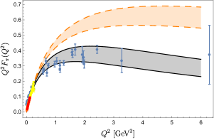
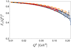
Figure 1: The pion ff Eq. (40). Full lines for the GSWL2 model and dashed lines for the GSWL1 model. Data from Refs. [48, 49, 50, 51, 52, 53, 54]. Left panel for $Q^{2}F_{\pi}(Q^{2})$. Right panel for $|F_{\pi}(Q^{2})|^{2}$. Bands stand for the error in $\alpha$.

6.3 The pion mean radius

A crucial quantity encoding the non perturtbative structure of the pion is the charge radius. This quantity can be extracted from the ff or directly from the LF wave function. In general one defines the mean square radius by,

$$\langle r^{2}\rangle_{\pi}=-6\dfrac{dF_{\pi}(Q^{2})}{dQ^{2}}\Big{|}_{Q^{2}=0}~{}.$$ (41)

As one can see in Tab. 2, both GSWL models are able to reproduce, within the uncertainty on $\alpha$, the data and the most recent extractions of the mean pion radius [55, 56]. The two parametrization are almost equivalent for this observable.

	Ref.	Ref.	Ref.	GSWL1	GSWL2	Experiment	Work of Ref.
	[26]	[57]	[58]			[55]	[56]
$\sqrt{\langle r^{2}\rangle}$ [fm]	0.524	0.673-0.684	0.644	$0.67\pm 0.03$	$0.70\pm 0.05$	0.67 $\pm 0.01$	$0.640\pm 0.007$

Table 2: Values of the pion mean radius obtained within different holographic models. Experimental data are from Ref. [55]. In the last column we report the recent analysis of Ref. [56].

6.4 The pion effective form factor

The pion effective form factor (eff) has been considered lately as a test for models [59]. Such a quantity has been introduced for the first time in the context of double parton scattering (DPS) processes in proton-proton collisions and double parton distribution functions (dPDFs) [60]. An overview about the study of DPS processes can be found in the seminal book Ref. [61]. In DPS two partons of an hadron interact with two partons of the other colliding hadron. For a long time, in order to estimate the DPS cross-section without any phenomenological information on dPDFs, a factorization ansatz of these quantities have been assumed for these quantity. Thanks to this strategy the DPS cross-section could be estimated from the the product of the two single parton scattering (SPS) cross-sections scaled by an almost theoretical unknown quantity called effective cross-section [62]:

$$\sigma^{A+B}_{DPS}\propto\dfrac{\sigma^{A}_{SPS}\sigma^{B}_{SPS}}{\sigma_{eff}}~{},$$ (42)

where $\sigma^{A+B}_{DPS}$ is the DPS cross-section for the production of two final states $A$ and $B$ respectively, and $\sigma^{A(B)}_{SPS}$ is the SPS cross-section for the production of the final state $A(B)$. Within this scheme, the effective cross-section, $\sigma_{eff}$, can be evaluated as follows:

$$\sigma_{eff}=\dfrac{1}{\displaystyle\int\dfrac{d\mathbf{k}_{\perp}}{(2\pi)^{2}}F_{2\pi}(k_{\perp}^{2})^{2}}~{},$$ (43)

where $F_{2\pi}(k_{\perp})$ is the eff and $\mathbf{k}_{\perp}$ is the conjugate variable to the transverse distance between two partons in the hadron. The eff can be obtained as the first moment of the dPDF [63], analogously to the form factor that can be obtained from the moments of the generalized parton distribution function [64]. In terms of the LF wf of the pion, the eff is defined as follows,

$$F_{2\pi}(k_{\perp}) =\int_{0}^{1}dx~{}\int{d^{2}{\bf k}_{\perp 1}\over 16\pi^{3}}~{}\psi_{2/h}^{*}(x,{\bf k}_{\perp 1})\psi_{2/h}(x,{\bf k}_{\perp 1}+{\bf k_{\perp}})$$ (44)

$$=\int_{0}^{1}dx~{}\int{d^{2}{\bf b_{\perp}}}~{}|\tilde{\psi}_{LF}(x,\mathbf{b}_{\perp})|^{2}e^{i\mathbf{k}_{\perp}\cdot\mathbf{b}_{\perp}}~{}.$$

In Ref. [63], the connection between the eff and the geometrical properties of the parent hadron have been established. In fact, the eff of the pion can be related to the mean transverse distance between two partons:

$$\langle b^{2}_{\perp}\rangle\simeq-4{dF_{2\pi}(k_{\perp})\over dk_{\perp}^{2}}\Bigg{|}_{k_{\perp}=0}~{},$$ (45)

where $k_{\perp}$ is the conjugate variable to $b_{\perp}$ and represents the momentum unbalance between the first and the second parton in the initial and final states in DPS processes. One of the first calculations of the pion dPDF is that of Ref. [65] where the SW model of Ref. [26] has been used. Thereafter a first evaluation of two-current correlations in the pion within lattice QCD [66] was carried out. Other studies of the pion eff and $\sigma_{eff}$ have been discussed in Refs. [59, 67, 68, 69].

Let us mention in particular the study of Ref. [59], where the pion effs evaluated with different holographic models have been compared with lattice QCD predictions in the allowed regions of $k_{\perp}^{2}$. Indeed, lattice calculations were performed in the pion rest frame [66] and the eff has been parametrized as follows:

$$F_{2\pi}(k_{\perp})=\dfrac{1}{\left[1+\langle b^{2}\rangle\dfrac{k_{\perp}^{2}}{6n}\right]^{n}}~{}.$$ (46)

A good fit to lattice data was obtained for $n=1.173$ and the extraction of the mean distance between two partons in the pion is $\sqrt{\langle b^{2}\rangle}=\sqrt{3/2\langle b_{\perp}^{2}\rangle}=1.046\pm 0.049$ fm [66]. This important result has been used to test holographic models of the pion [59]. As stressed in Ref. [59], lattice outcomes have been obtained in the pion rest frame. However, the comparison with holographic LF calculations is allowed in the Infinite Momentum Frame (IMF) which can be emulated by the kinematic condition: $k_{\perp}^{2}<<m_{\pi}^{2}\sim 0.3^{2}$ GeV².

In Ref. [59] it has been thoroughly discussed the difficulties in describing the ff and the eff with the same parameters in a given model. Such a result led to the conclusion that more sophisticated models are necessary to reproduce the ff and the eff. In the present analysis, the GSWL1 and GSWL2 parametrization were used to evaluate Eqs. (44, 45). In Fig. 2 the square of the pion eff is displayed showing the comparison between lattice data and our model calculations. Let us stress that since the DPS cross-section, even in the simplified description of Eq. (42) depends on the square of the eff, in Fig. 2 we report such a quantity, instead of the eff, in order to highlight the relevant differences that could affect the evaluation of experimental observables, such as $\sigma_{eff}$. As one can see, in this case the GSWL1 model is able to reproduce the lattice data with impressive accuracy. On the other hand the GSWL2, although it provides a reasonable agreement, it underestimates slightly this quantity. We show in Fig. 3, extracted from Ref. [59], the results of other model calculations. It can be noted, that despite the limited success of the SW model in describing the pion ff, such a model is capable of describing the eff lattice data. Such feature is shared with the GSWL1 parametrization, where the ff is not overall well reproduced but the eff is close to lattice data. On the contrary the GSWL2 model, which describes well the experimental data of the ff, underestimates the eff lattice data. Finally, in Tab. 3 we compare the mean distance between two partons in the pion evaluated in different models with the lattice predictions. In this case, the pion GSWL1 parametrization, without any dedicated parameter, is the only model that reproduces the lattice data within error. Also the GSWL2 predicts a value for this quantity close to the data.

The calculation of the eff confirms again the difficulty in reproducing the mean pion charge radius and the mean distance between two partons in the pion with the same parameters, . However, at variance with the SW model which leads to a good value for this distance but fails in evaluating $\sqrt{\langle r^{2}\rangle}$, the GSWL1 is able to reproduce simultaneously $\sqrt{\langle r^{2}\rangle}$ and $\sqrt{\langle b^{2}\rangle}$. Coherently with the eff analysis, the GSWL2 is not able to reproduce the mean distance with an error very close to that of the SW calculation. However, the GSWL2 model calculation of the pion charge radius matches the data.

In closing this section the analysis of the data so far of all the holographic models allows us to conclude that the GSWL1 and GSWL2 parametrizations are capable of describing reasonably well the one-body and two-body ffs simultaneously. From this point of view the graviton soft-wall model including the longitudinal dynamics is very promising in describing the DPS pion physics.

	Model of Ref.	Model of Ref.	Model of Ref.	Lattice	GSWL1	GSWL2
	[26]	[57]	[58]	[66]
$\sqrt{\langle b^{2}\rangle}$ [fm]	0.968	1.207	0.767	1.046 $\pm 0.049$	$1.13\pm 0.06$	$1.24\pm 0.08$

Table 3: Values of the mean partonic distance in the pion, Eq. (45), obtained in lattice QCD [66] and in models based on the AdS/QCD approach [26, 57, 58].

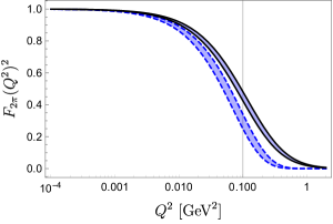
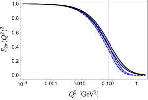
Figure 2: The square of the eff Eq. (44). Full lines represent lattice data [66] and the band stands for the error in the mean distance entering the lattice pasteurization, see Eq. (46). Left panel the same observable for the GSWL2. Right panel the same for the GSWL1.

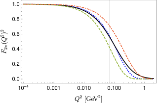
Figure 3: Same of Fig. 2 from Ref. [59]. Full line the lattice calculation. Dot-dashed line calculation for the model of Ref. [58]. Dotted line for the model of Ref. [26] and dashed line for that of Ref. [57].

6.5 The pion decay constant

In this section results for the calculation of the pion decay constant are presented and discussed. This quantity can be defined from the parametrization of the Lorentz structure of the following amplitude:

$$\langle 0|\bar{\psi}\gamma^{+}\dfrac{1}{2}(1-\gamma_{5})\psi|\pi\rangle=i\dfrac{P^{+}f_{\pi}}{\sqrt{2}}~{}.$$ (47)

Thanks to the LF wf representation of the pion state, leading to the Fock expansion previously described, one can relate the pion decay constant to its LF wf [70, 26]:

$$f_{\pi}=2\sqrt{N_{C}}\int_{0}^{1}dx~{}\int\dfrac{d\mathbf{k}_{\perp 1}}{16\pi^{3}}\psi_{2/h}(x,\mathbf{k}_{\perp 1})~{}.$$ (48)

In order to avoid confusion with other definitions, used in e.g. Ref. [71], let us specify that within the present formalism we consider the experimental data [34] $(130\pm 5)/\sqrt{2}=91.92\pm 3.54$ MeV. Comparisons with data and other model calculations [22, 26, 57] are displayed in Tab. 4. We stress again that the quoted value in that references might be rescaled by a factor $1/\sqrt{2}$ when needed. As one can see, holographic approaches are qualitatively able to describe the decay constant. In order to highlight the discrepancy with the data and model predictions, the quantity $\Delta_{\pi}=|f_{\pi}^{holo}-f_{\pi}^{exp}|$ is shown in Tab. 4. As one can see the GSWL2 parametrization and the model of Ref. [57] is quite close to the data. In this case, a bigger discrepancy is found for the GSWL1 case, although the result is not too distant from the data.

	Data [34]	GSWL1	GSWL2	Work of Ref. [22]	SW [26]	Work of Ref. [57]
$f_{\pi}$ [MeV]	$91.92\pm 3.54$	$126\pm 6$	$104\pm 7$	129	81.2	95.5-97.6
$\Delta_{\pi}$ [MeV]		$34\pm 7$	$12\pm 8$	$37.1\pm 3.5$	$11\pm 4$	$3.1\pm 3.5-5.7\pm 3.5$

Table 4: Comparison of the pion decay constant between holographic models [26, 57] and data [34]. The difference in modulus between the experimental value and the model predictions is display in the last line.

6.6 The pion distribution amplitude

In this section we provide the calculation of the pion distribution amplitude (DA) with the Light-Front formalism for the GSWL models. There are many for DA and we choose the one of Ref.  [26, 70]

$$\phi(x;Q)=\int_{0}^{Q^{2}}\dfrac{d^{2}\mathbf{k}_{\perp 1}}{16\pi^{3}}\psi_{2/\pi}(x,\mathbf{k}_{\perp 1})~{}.$$ (49)

We stress that, in analogy with the SW results, also in the GSWL models the soft $Q^{2}$ dependence, due to the wf dependence on the transverse momentum, can be safely neglected for $Q^{2}>1$ GeV². Thanks to this choice, the present evaluation can be compared to the asymptotic expression for the DA [70, 72, 73]:

$$\phi^{asy}_{pQCD}=\sqrt{3}f_{\pi}x(1-x)~{}.$$ (50)

We also display the DA obtained within the SW model of Ref. [26],

$$\phi_{AdS}^{asy}(x)=4f_{\pi}\sqrt{x(1-x)}/(\sqrt{3}\pi)$$ (51)

One should notice that in the asymptotic regime, the scale dependence of the model disappears. Therefore the DA evaluated with the SW model of Ref. [26] and discussed in Ref. [74], is the same as that obtained with the GSW model not including the longitudinal dynamics. On the other hand, the GSWL prediction for the DA, in the mentioned region is

$$\phi^{asy}_{GSWL}\propto\big{[}x(1-x)\big{]}^{\frac{1}{2}+\frac{m_{q}}{\sigma}~{},}$$ (52)

where for the GSWL1 parametrization the exponential is 0.852 while for the GSWL2 parametrization is 1.12. The models which incorporate longitudinal dynamics produce an $x$ dependence of the DA in closer agreement with the pQCD asymptotic behaviour than the SW model of Ref. [26]. Such features can be observed in the left panel of Fig. 4.

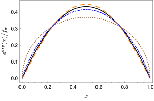
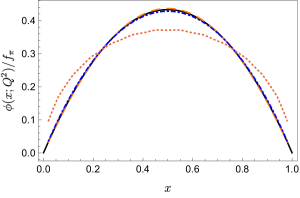
Figure 4: The pion DA. Full lines represent the asymptotic pQCD prediction whose expression is in Eq. (50). Dashed lines for the GSWL2 parametrization. Dot-Dashed line for GSWL1 and dotted lines for the GSW and SW [74] models, see Eq. (51). Left panel: calculations of the DA in the asymptotic limit without evolution. Right panel the same as the left panel but including the ERBL evolution for $Q^{2}=1.5$ GeV².

6.6.1 Evolution of the DA

As discussed in Ref. [74], the $Q^{2}$ dependence of the DA has two sources: $i)$ the soft one, due to the integration of the wf up to the scale $Q^{2}$, see Eq. (49), and $ii)$ the hard one, due to the ERBL evolution of the DA [70, 75]. In fact, within the SW and GSW models, in general one could write the DA, including the soft $Q^{2}$ dependence as follows:

$$\phi(x;Q^{2})=\phi^{asy}(x)\phi_{soft}(x,Q^{2})=\phi^{asy}(x)\left[1-exp\left(-\dfrac{Q^{2}}{\kappa^{2}\sqrt{-2+\dfrac{1-2\gamma}{\alpha^{2}}}x(1-x)}\right)\right]~{},$$ (53)

where, in the case of the GSW model, $\kappa^{2}=0.37^{2}/\sqrt{\alpha}$ GeV². From the above equation it is clear that from the model calculation of $\phi$ one gets $\phi^{asy}$ by considering that $\phi^{asy}(x)=\phi(x,Q^{2}\rightarrow\infty)$. In this case, this soft dependence is almost negligible for $Q>$1 GeV. In order to properly take into account also the perturbative QCD effects, the distribution $\phi^{asy}(x)=\phi^{asy}(x,\mu_{0})$ appearing in Eq. (53) must be evolved by using the ERBL evolution of the DA.

We recall that due to ERBL evolution at a given final momentum scale the DA reads,

$$\phi^{asy}(x;Q)=x(1-x)\sum_{n=0,2,4...}^{\infty}a_{n}(Q)C^{3/2}_{n}(2x-1)~{},$$ (54)

where here $C_{n}^{\alpha}(x)$ are Gegenbauer polynomials and

$$a_{n}(Q)=\left[\dfrac{\alpha_{s}(\mu_{0}^{2})}{\alpha_{s}(Q^{2})}\right]^{\gamma_{n}/\beta_{0}}a_{n}(\mu_{0})~{}.$$ (55)

In the above expressions the following quantities appear

$$\beta_{0}=11-\dfrac{2}{3}n_{f}$$ (56)

$$\alpha_{s}(Q^{2})=\dfrac{4\pi}{\beta_{0}\ln(Q^{2}/\Lambda_{QCD}^{2})}$$ (57)

$$\gamma_{n}=\dfrac{4}{3}\left[3+\dfrac{2}{(n+1)(n+2)}-4\sum_{j=1}^{n+1}\dfrac{1}{j}\right]~{},$$ (58)

$$a_{n}(\mu_{0})=\dfrac{4(2n+3)}{(n+2)(n+1)}\int_{0}^{1}dx~{}\phi^{asy}(x,\mu_{0})C_{n}^{3/2}(1-2x)~{},$$ (59)

where $n_{f}=3$ and $\Lambda_{QCD}\sim 0.225$ GeV. Finally, once the the soft and hard $Q^{2}$ parts are separated, the total evolved DA is given by

$$\phi(x;Q^{2})=\phi^{asy}(x;Q^{2})\phi_{soft}(x;Q^{2})~{}.$$ (60)

In analogy with Refs. [71, 74], we fix the initial scale of the model by comparing the evolution of parton distribution functions with the corresponding data. In particular, as will be properly discussed in a next subsection, we consider $0.07\leq\mu_{0}^{2}\leq 0.11$ GeV². In the left panel of Fig. 4, the asymptotic DA evaluated with the SW model [74] and the GSWL models, is compared with the pQCD predictions. Effects of ERBL evolution of the DA are shown in the right panel of Fig. 4. Here we display the DA evolved to $Q^{2}=1.5$ GeV² from $\mu_{0}^{2}=0.07$ GeV² for the GSWL1 and GSWL2 parametrizations. The evolution brings the DA towards the pQCD asymptotic limit. This feature is due to the power of the exponential which, in the GSWL models, is close to the pQCD prediction already at the initial scale. In Fig. 5 we compare the normalized DA with the data of Ref. [76]. As one can see good agreement is obtained. Let us specify that the DA appearing in Fig. 5 can be obtained from that satisfying Eq. (49) with a simple re-scaling so that:

$$\int dx~{}\phi(x;Q^{2})_{norm}=1~{}.$$ (61)

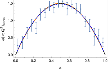
Figure 5: Comparison between the normalized DA, see Eq. (61) and the data from Ref. [76]. The final scale is $Q=3.16$ GeV. The full line shows the pQCD prediction. The dashed line corresponds to the GSWL2 parametrization and the dot-dashed line is related to the GSWL1 one.

An important test for the DA is represented by the moments of the DA:

	$\langle z^{2}\rangle$	$\langle z^{4}\rangle$	$\langle z^{6}\rangle$	$\langle z^{-1}\rangle$
Asymptotic	0.200	0.086	0.048	3.000
Ref. [71]	0.217	0.097	0.055	3.170
Ref. [77]	$0.24\pm 0.22$	$0.11\pm 0.09$	$0.07\pm 0.05$
Ref. [74]	0.25	0.125	0.078	3.98
Ref. [57]	0.185	0.071		2.85
Ref. [57]	0.200	0.085		2.95
Lattice
Ref. [78]	$0.28^{+0.01}_{-0.01}$
Ref. [79]	$0.2361^{+0.0041}_{-0.0039}$
Ref. [80]	$0.27\pm 0.04$
Ref. [81]	$0.2077\pm 0.0043$
Ref. [82]	$0.234\pm 0.006$
Ref. [83]	$0.244\pm 0.030$
GSWL1	$0.2033\pm 0.0007$	$0.0880\pm 0.0005$	$0.0493\pm 0.0004$	$3.0349\pm 0.0087$
GSWL2	$0.19770\pm 0.0005$	$0.0841\pm 0.0004$	$0.0465\pm 0.0002$	$2.9770\pm 0.0055$

Table 5: Comparison between the moments of the DA evaluated with the GSWL models and other approaches. The error in the GSWL1 and GSWL2 models is due to the uncertainty of the initial scale $0.07\leq\mu_{0}^{2}\leq 0.1$.

$$\langle z^{p}\rangle=\dfrac{\displaystyle\int_{0}^{1}dx~{}z^{p}\phi(x,Q^{2})}{\displaystyle\int_{0}^{1}dx~{}\phi(x,Q^{2})}~{}$$ (62)

where $z=2x-1$ for $p\geq 1$ and $z=x$ for $p=-1$. As one can see in Tab. 5, the GSWL models produce results close to the pQCD predictions, as expected from the power behaviour of the DA, Eq. (52), as compared to that of Eq. (50). In all cases, the results are close to the other phenomenological models. Let us mention that numerically, results displayed in Tab. 5, obtained within the GSWL models, are consistent with the alternative expression of the DA moments [77] (see Appendix A):

$$\langle z^{2}\rangle =\dfrac{6}{a_{0}(Q)}\left(\dfrac{2}{35}a_{2}(Q)+\dfrac{1}{30}a_{0}(Q)\right)$$ (63)

$$\langle z^{4}\rangle =\dfrac{6}{a_{0}(Q)}\left(\dfrac{4}{231}a_{4}(Q)+\dfrac{4}{105}a_{2}(Q)+\dfrac{1}{70}a_{0}(Q)\right)$$

$$\langle z^{6}\rangle =\dfrac{6}{a_{0}(Q)}\left(\dfrac{32}{6435}a_{6}(Q)+\dfrac{20}{1001}a_{4}(Q)+\dfrac{2}{77}a_{2}(Q)+\dfrac{1}{1260}a_{0}(Q)\right)~{}.$$

6.7 Pion-photon transition form factor

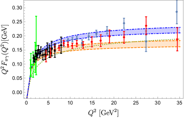
Figure 6: The pion to photon transition form factor, Eq. (65) evaluated within the GSWL2 (dashed) and GSWL1 (dot-dashed) parametrizations. The dotted line stands for the SW prediction. Data are collected from Refs. [84, 85, 86, 87]. The initial scale is $\mu_{0}^{2}=0.07$ GeV².

In this section we discuss the calculation of the pion-photon transition form factor. Such a quantity is relevant for processes, e.g., $\gamma^{*}(q)\gamma\rightarrow\pi^{0}$ and can be defined through the matrix element of the following electromagnetic current [70]:

$$\langle\gamma(P-q)|J^{\mu}|\pi(P)\rangle=ie^{2}F_{\gamma\pi}(Q^{2})\varepsilon^{\mu\nu\rho\sigma}P_{\nu}\varepsilon_{\rho}q_{\sigma}~{},$$ (64)

where $P$ is the pion 4-momentum, $q=-Q$ is the photon virtuality and $\varepsilon_{\rho}$ is the polarization vector. At LO, the transition ff can be evaluated from the DA convoluted with a specific kernel [88, 89, 74]:

$$Q^{2}F_{\gamma\pi}(Q^{2}) =\dfrac{4}{\sqrt{3}}\int_{0}^{1}dx~{}T_{H}(x,Q^{2})\int_{0}^{\bar{Q}}\dfrac{d\mathbf{k}_{\perp 1}}{16\pi^{3}}\psi_{2/\pi}(x,\mathbf{k}_{\perp 1})$$ (65)

$$=\dfrac{4}{\sqrt{3}}\int_{0}^{1}dx~{}T_{H}(x,Q^{2})\phi(x,\bar{Q})~{}$$

where here $\bar{Q}=(1-x)Q$ and at LO

$$T^{LO}_{H}(x,Q^{2})=\dfrac{1}{1-x}$$ (66)

while at NLO

$$T^{NLO}_{H}(x,Q^{2})=T_{H}^{LO}(x,Q^{2})\left[1-\dfrac{\alpha(Q^{2})}{4\pi}C_{f}\left(9+\dfrac{1-x}{x}\log(1-x)-\log(1-x)^{2}\right)\right]~{},$$ (67)

where further logarithms are neglected by setting the regularization scale to be equal to $Q$ [74, 71]. In the asymptotic limit one should approach the pQCD prediction: $Q^{2}F_{\gamma\pi}(Q^{2})\rightarrow 2f_{\pi}$ [74]. Deviation from the latter condition are expected from model calculations that differ from the well known DA $\phi(x)\sim x(1-x)$ in the asymptotic region. In Fig. 6 the transition ff, Eq. (65), is shown for both the GSWL reparametrizations. To this aim the DA has been evolved by properly taking into account the soft and hard $Q^{2}$ dependences. Such an approach has been investigated in detail in Ref. [74]. The above quantity has been obtained for $\mu_{0}^{2}=0.07$ GeV². No relevant differences are found for $0.07\leq\mu_{0}^{2}\leq 0.11$ GeV². As one can see in Fig. 6 the data [84, 85, 86, 87] are well reproduced. From a numerical point of view, in order to guarantee the convergence of the integral Eq. (65), we need to impose that for $(1-x)Q<\mu_{0}$ then $\bar{Q}=\mu_{0}$  [74, 71]. While the SW model is not able to describe the data the GSWL models do well.

6.8 Virtual photon transition form-factor

We present also the calculation of the transition ff for a pion which decays in two virtual photons: $\pi^{0}\rightarrow\gamma^{*}\gamma^{*}$. This quantity now depends on the virtualities of the two photons $Q_{1},Q_{2}$ [70, 90],

$$F_{\pi\gamma^{*}}(Q_{1}^{2},Q^{2}_{2})=\dfrac{2}{\sqrt{3}}\int_{0}^{1}dx~{}\bar{T}_{H}(x,Q_{1}^{2},Q^{2}_{2})\phi(x,W)~{},$$ (68)

where $\bar{T}_{H}(x,Q_{1}^{2},Q^{2}_{2})$ is the hard-scattering amplitude for the present process. At LO:

$$\bar{T}_{H}^{LO}(x,Q_{1}^{2},Q^{2}_{2})=\dfrac{1}{(1-x)Q_{1}^{2}+xQ_{2}^{2}}~{},$$ (69)

while at NLO the kernel has been derived in Ref. [91] and we show it in appendix A. One should notice that the transition ff with a real photon is obtained for $Q_{1}=0$ or $Q_{2}=0$. In addition, at LO, for $Q_{1}=Q_{2}$, the amplitude does not depend on $x$, and therefore one gets $Q^{2}F_{\pi\gamma^{*}}(Q^{2},Q^{2})\rightarrow\sqrt{2}/3f_{\pi}$. In Fig. 7 the results with the GSWL parametrizations are compared with NLO pQCD calculations. As one can see the second parametrization GSWL2 provides the expected results within the theoretical error in $\alpha$. On the other hand GSWL1 overestimates the pQCD result. Nevertheless, since in the asymptotic regions, for $Q_{1}=Q_{2}$, this ff is proportional to the decay constant, in order to exclude from the calculations the error related to this quantity, in Fig. 8 we plot $F_{\pi\gamma^{*}}/f_{\pi}$. As one can see, for both the GSWL parametrizations, the model is able to reproduce the pQCD predictions which are determined by both the NLO correction to the kernel Eq. (69) and the ERBL evolution of the DA. The scaling behavior $F_{\pi\gamma^{*}}(Q_{1}^{2},Q_{2}^{2})\sim 1/(Q_{1}^{2}+Q_{2}^{2})$ is verified.

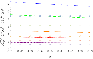
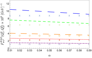
Figure 7: The pion virtual photon transition form factor evaluated at NLO as a function of the parameter $\alpha$. Lines stand for the GSWL calculations and markers for the pQCD predictions [71]. Long dashed blue line and blue crossed points for $(Q_{1}^{2}=Q_{2}^{2}=6.48)$ GeV². Middle dashed orange line and orange circle points for $(Q_{1}^{2}=Q_{2}^{2}=16.85)$ GeV². Small dashed green line and green square points for $(Q_{1}^{2}=14.83;~{}Q_{2}^{2}=4.27)$ GeV². Dotted red line and red star points for $(Q_{1}^{2}=38.11;~{}Q_{2}^{2}=14.95)$ GeV². Dot-Dashed purple line and purple triangle points for $(Q_{1}^{2}=Q_{2}^{2}=45.63)$ GeV². Left panel for GSWL1. Right panel for GSWL2.

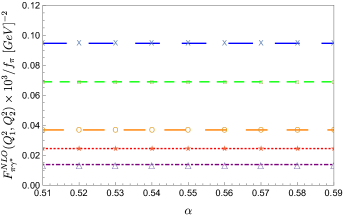
Figure 8: Same of fig. 7 but for $F_{\pi\gamma^{*}}/f_{\pi}$.

6.9 The pion parton distribution function

In this last section we present the calculation of the parton distribution function of the pion. These quantities can be defined in terms of the LF wf,

$$f(x;\mu_{0}^{2})=\int\dfrac{d\mathbf{k}_{\perp 1}}{16\pi^{3}}|\psi_{2/\pi}(x,\mathbf{k}_{\perp})|^{2}=[(1-x)x]^{2m_{q}/\sigma}\dfrac{\Gamma\left[2+\dfrac{4m_{q}}{\sigma}\right]}{\Gamma\left[1+\dfrac{2m_{q}}{\sigma}\right]^{2}}~{}.$$ (70)

Several analyses have been performed within holographic models, see e.g. Refs. [58, 57, 92, 93]. Let us also mention predictions from QFT based models such those of, e.g. Refs. [94, 95].

Let us recall that, if only the LF wf determined by the modes of the pseudo-scalar field, propagating in the modified metric, are considered, the PDF will be constant, as discussed for the SW model of Ref. [74]. Therefore, in this investigation, we take advantages of the longitudinal dynamics introduced in order to describe the chiral symmetry breaking. Such feature leads to a complex structure of the pion already appreciated in the study of the ff. In this case the GSWL1 parametrization leads to the following PDF

$$f(x;\mu_{0}^{2})=3.63798[(1-x)x]^{0.704348}~{}$$ (71)

while the GSWL2 parametrization to the following

$$f(x;\mu_{0}^{2})=8.7889[(1-x)x]^{1.23133}~{}.$$ (72)

Let us remark that the GSWL2 parametrization predicts that $f(x\rightarrow 1)\sim(1-x)^{1.23133}$, such an exponent is close to that found in e.g. Refs. [93, 94] and in phenomenological studies such as in Ref. [96].

As already discussed, the initial scale is fixed by fitting the data of Ref. [97] obtained at the final scale $\mu^{2}=27$ GeV². We consider here leading order (LO) pQCD evolution of the pion PDF. In Fig. 9 one can see that both parametrizations are almost able to describe the data in the valence region for small initial scales, as expected for a LO calculation. However, in order to describe the data, higher values of $\mu_{0}^{2}$ are needed. In Fig. 9 we display the results for $0.07\leq\mu_{0}^{2}\leq 0.15$ GeV². One should notice that the allowed range of initial scales here considered are similar to those usually adopted by constituent quark models, namely when only the constituent quarks carry all the momentum of the parent hadron. Thus, to conclude, we can safely state that the GSW model, including the longitudinal dynamics, is a very promising model to investigate the pion structure functions.

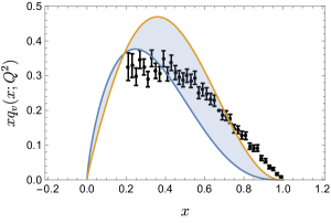
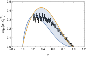
Figure 9: The pion PDF evaluated at LO to the final scale $\mu^{2}=27$ GeV². The band stands for the uncertainty related to initial scale $0.07\leq\mu_{0}^{2}\leq 0.15$ GeV². Data are from Ref. [97]. Left panel for the GSWL1 reparametrization. Right panel for the GSWL2 parametrization.

7 Conclusion

The GSW model was born to describe the scalar and tensor glueballs in $AdS_{5}$ space. It is characterized by a warped metric and the description of these glueballs as gravitons in five dimensions  [5, 6, 7]. The model has been improved and extended to describe all mesons and glueballs [8]. In the latter study we appreciated that the ground state of the pion was very peculiar and required a special dilaton in order to achieve its low mass. This feature is associated with the realization of chiral symmetry in QCD and certainly our previous procedure, describing this mechanism with a sophisticated dilaton, produced a pion spectrum which had many intermediate states [8], which in some sense was contradicting the data, although one must be aware that the data have a complicated structure which could hide these intermediate states. Moreover, the wave function we could derive from its mode function is not able to provide many observables with precision.

In this work we have adopted a different approach closer to the realization of chiral symmetry in QCD. For that purpose we have introduced via dilatons the appropriate scales to generate a massless pion. Thereafter we break explicitly chiral symmetry by introducing massive quarks via longitudinal dynamics, as proposed in Refs. [22, 23]. With this modification we successfully reproduced the spectrum with the addition of a well known longitudinal potential with only two additional parameters, a constituent quark mass $m_{q}$ and a correction to the energy scale $\gamma_{\pi}$ to generate the adequate mass gaps of the excitations.

Having this model for the pion we have proceeded to calculate many pion observables with only these two parameters. We discussed two different characterizations which have almost the same quark mass but quite different $\gamma_{\pi}$. The relation between the observables and the parametrizations is highly non linear. The studied observables comprise low energy as well as high energy properties. We have implemented evolution, using the model calculations at a low momentum scale, in order to be able to compare with perturbative QCD results.

The main conclusion of our investigation is that, although each parametrization does better in some observables than the other, on the overall, both parametrizations lead to a good qualitative description of all the observables.

Appendix A

Here we explicitly show how to derive the relations between th moments of the DA, see Eq. (62) and the coefficients of the ERBL evolution expansion, see Eqs. (55-59). The result of this procedure is described in Eq. (63). We remark that since we are interested in moments at high energy scales, the soft part of the DA can be neglected, see Eq. (50). In order to fulfill this properties, already discussed in Ref. [77], we consider that,

$$\int_{0}^{1}dx~{}\phi(x;Q^{2}) =\sum_{n}a_{n}(Q^{2})\int_{0}^{1}x(1-x)C_{n}^{3/2}(2x-1)$$ (73)

$$=\sum_{n}a_{n}(Q^{2})\dfrac{1}{6}\delta_{n0}=\dfrac{a_{0}(\mu_{0}^{2})}{6}$$

$$=\int_{0}^{1}dx~{}\phi^{asi}(x;\mu_{0}^{2})=\dfrac{f_{\pi}}{2\sqrt{3}}~{}.$$

Then for $\langle z^{2}\rangle$ we have:

$$\int_{0}^{1}dx~{}(2x-1)^{2}\phi(x;Q^{2}) =\sum_{n}a_{n}(Q^{2})\int_{0}^{1}(2x-1)^{2}x(1-x)C_{n}^{3/2}(2x-1)$$ (74)

$$=\sum_{n}a_{n}(Q^{2})\left[\dfrac{2}{35}\delta_{n2}+\dfrac{1}{30}\delta_{n0}\right]$$

$$=\dfrac{2}{35}a_{2}(Q^{2})+\dfrac{1}{30}a_{0}(Q^{2})~{}.$$

Recursively one would get:

$$\dfrac{\displaystyle\int_{0}^{1}dx~{}(2x-1)^{2l}\phi(x;Q^{2})}{\displaystyle\int_{0}^{1}dx~{}\phi(x;Q^{2})}=6\sum_{n}^{2l}\dfrac{a_{n}(Q^{2})}{a_{0}(Q^{2})}\int_{0}^{1}(2x-1)^{2l}x(1-x)C_{n}^{3/2}(2x-1)~{}.$$ (75)

Appendix A

In this section we show the the kernel of the transition form factor for two virtual photon produced of momenta $q_{1}^{2}=-Q_{1}^{2}$ and $q_{2}^{2}=-Q_{2}^{2}$, respectively. In particular we consider the NLO calculation discussed in Ref. [91] and used in Refs. [71, 98]. To this aim let us define $Q^{2}=Q_{1}^{2}+Q_{2}^{2}$, $w=Q_{1}^{2}/Q^{2}$ and $z=(1-x)w+x(1-w)x$. The kernel $\bar{T}^{NLO}_{H}$ is obtained from:

$$t(x,w) =\left[\dfrac{w-x}{2x-1}-\left(\dfrac{z}{2w-1}\right)^{2}\right]\left[\dfrac{L_{1}L_{3}}{x}+\dfrac{L_{2}L_{3}}{1-x}-\dfrac{L_{1}^{2}}{2x}-\dfrac{L_{2}^{2}}{2(1-x)}\right]$$ (76)

$$+\dfrac{1-z}{2(2w-1)}(L_{1}-L_{2})(2L_{3}-L_{1}-L_{2})+\dfrac{3}{2}(L_{3}-3)$$

$$-\left[\dfrac{3}{2}\dfrac{w-x}{2w-1}-\left(\dfrac{z}{2w-1}\right)^{2}\right]\left[\dfrac{L_{1}}{x}+\dfrac{L_{2}}{1-x}\right]-\dfrac{1}{2}\dfrac{3-2z}{2w-1}(L_{1}-L_{2})~{},$$

where:

$$L_{1} =\log\left(\dfrac{z}{w}\right)$$ (77)

$$L_{2} =\log\left(\dfrac{z}{1-w}\right)$$ (78)

$$L_{3} =\log\left(z\right)~{}.$$ (79)

Then one can build

$$T(Q,w,x)=\dfrac{1}{Q^{2}}\dfrac{}{(1-x)w+x(1-w)}\left[1+C_{F}\dfrac{\alpha_{s}(Q^{2})}{2\pi}t(x,w)\right]$$ (80)

from which the NLO kernel is obtained via symmetrization:

$$\bar{T}_{H}^{NLO}(x;Q_{1}^{2},Q_{2}^{2})=\dfrac{T(Q,w,x)+T(Q,w,1-x)}{2}~{}.$$ (81)

We recall that also in this case other logarithms are neglected by setting $Q$ equal to the regularization scale.

References

- [1] Juan Martin Maldacena. The Large N limit of superconformal field theories and supergravity. Int. J. Theor. Phys., 38:1113–1133, 1999. [Adv. Theor. Math. Phys.2,231(1998)].
- [2] Edward Witten. Anti-de Sitter space, thermal phase transition, and confinement in gauge theories. Adv. Theor. Math. Phys., 2:505–532, 1998.
- [3] H. Fritzsch, Murray Gell-Mann, and H. Leutwyler. Advantages of the Color Octet Gluon Picture. Phys. Lett., 47B:365–368, 1973.
- [4] Harald Fritzsch and Peter Minkowski. Heavy Elementary Fermions and Proton Stability in Unified Theories. Phys. Lett., 56B:69–72, 1975.
- [5] Matteo Rinaldi and Vicente Vento. Scalar and Tensor Glueballs as Gravitons. Eur. Phys. J., A54:151, 2018.
- [6] Matteo Rinaldi and Vicente Vento. Pure glueball states in a Light-Front holographic approach. J. Phys., G47(5):055104, 2020.
- [7] Matteo Rinaldi and Vicente Vento. Scalar spectrum in a graviton soft wall model. J. Phys., G47(12):125003, 2020.
- [8] Matteo Rinaldi and Vicente Vento. Meson and glueball spectroscopy within the graviton soft wall model. Phys. Rev. D, 104(3):034016, 2021.
- [9] Joseph Polchinski and Matthew J. Strassler. The String dual of a confining four-dimensional gauge theory. 2000.
- [10] Stanley J. Brodsky and Guy F. de Teramond. Light-front hadron dynamics and AdS/CFT correspondence. Phys. Lett., B582:211–221, 2004.
- [11] Leandro Da Rold and Alex Pomarol. Chiral symmetry breaking from five dimensional spaces. Nucl. Phys., B721:79–97, 2005.
- [12] Andreas Karch, Emanuel Katz, Dam T. Son, and Mikhail A. Stephanov. Linear confinement and AdS/QCD. Phys. Rev., D74:015005, 2006.
- [13] Joshua Erlich, Emanuel Katz, Dam T. Son, and Mikhail A. Stephanov. QCD and a holographic model of hadrons. Phys. Rev. Lett., 95:261602, 2005.
- [14] Tony Gherghetta, Joseph I. Kapusta, and Thomas M. Kelley. Chiral symmetry breaking in the soft-wall AdS/QCD model. Phys. Rev., D79:076003, 2009.
- [15] Alfredo Vega and Paulina Cabrera. Family of dilatons and metrics for AdS/QCD models. Phys. Rev., D93(11):114026, 2016.
- [16] Tadakatsu Sakai and Shigeki Sugimoto. Low energy hadron physics in holographic QCD. Prog. Theor. Phys., 113:843–882, 2005.
- [17] Johannes Hirn and Veronica Sanz. Interpolating between low and high energy QCD via a 5-D Yang-Mills model. JHEP, 12:030, 2005.
- [18] Johannes Hirn and Veronica Sanz. The A(5) and the pion field. Nucl. Phys. B Proc. Suppl., 164:273–276, 2007.
- [19] Gerard ’t Hooft. A Two-Dimensional Model for Mesons. Nucl. Phys. B, 75:461–470, 1974.
- [20] Yang Li, Pieter Maris, Xingbo Zhao, and James P. Vary. Heavy Quarkonium in a Holographic Basis. Phys. Lett. B, 758:118–124, 2016.
- [21] M. Burkardt. Mesons in a collinear QCD model. Phys. Rev. D, 56:7105–7118, 1997.
- [22] Yang Li and James P. Vary. Light-front holography with chiral symmetry breaking. Phys. Lett. B, 825:136860, 2022.
- [23] Guy F. de Teramond and Stanley J. Brodsky. Longitudinal dynamics and chiral symmetry breaking in holographic light-front QCD. Phys. Rev. D, 104(11):116009, 2021.
- [24] Stanley J. Brodsky, Hans-Christian Pauli, and Stephen S. Pinsky. Quantum chromodynamics and other field theories on the light cone. Phys. Rept., 301:299–486, 1998.
- [25] Stanley J. Brodsky and Guy F. de Teramond. Hadronic spectra and light-front wavefunctions in holographic QCD. Phys. Rev. Lett., 96:201601, 2006.
- [26] Stanley J. Brodsky and Guy F. de Teramond. Light-Front Dynamics and AdS/QCD Correspondence: The Pion Form Factor in the Space- and Time-Like Regions. Phys. Rev., D77:056007, 2008.
- [27] Oleg Andreev. 1/q**2 corrections and gauge/string duality. Phys. Rev. D, 73:107901, 2006.
- [28] Eduardo Folco Capossoli and Henrique Boschi-Filho. Glueball spectra and Regge trajectories from a modified holographic softwall model. Phys. Lett., B753:419–423, 2016.
- [29] Eduardo Folco Capossoli, Miguel Angel Martin Contreras, Danning Li, Alfredo Vega, and Henrique Boschi-Filho. Hadronic spectra from deformed AdS backgrounds. Chin. Phys., C44(6):064104, 2020.
- [30] Miguel Angel Martin Contreras, Eduardo Folco Capossoli, Danning Li, Alfredo Vega, and Henrique Boschi-Filho. Pion form factor from an AdS deformed background. Nucl. Phys. B, 977:115726, 2022.
- [31] Kazuo Ghoroku, Nobuhito Maru, Motoi Tachibana, and Masanobu Yahiro. Holographic model for hadrons in deformed AdS(5) background. Phys. Lett. B, 633:602–606, 2006.
- [32] P. Colangelo, F. De Fazio, F. Jugeau, and S. Nicotri. On the light glueball spectrum in a holographic description of QCD. Phys. Lett., B652:73–78, 2007.
- [33] Miguel Angel Martin Contreras, Alfredo Vega, and Santiago Cortes. Light pseudoscalar and axial spectroscopy using AdS/QCD modified soft wall model. Chin. J. Phys., 66:715–723, 2020.
- [34] M. Tanabashi et al. Review of Particle Physics. Phys. Rev., D98(3):030001, 2018.
- [35] P. A. Zyla et al. Review of Particle Physics. PTEP, 2020(8):083C01, 2020.
- [36] M. Diehl, T. Feldmann, R. Jakob, and P. Kroll. The overlap representation of skewed quark and gluon distributions. Nucl. Phys. B, 596:33–65, 2001. [Erratum: Nucl.Phys.B 605, 647–647 (2001)].
- [37] Stanley J. Brodsky and Guy F. de Teramond. Light-Front Dynamics and AdS/QCD Correspondence: Gravitational Form Factors of Composite Hadrons. Phys. Rev., D78:025032, 2008.
- [38] Guy F. de Teramond and Stanley J. Brodsky. Light-Front Holography: A First Approximation to QCD. Phys. Rev. Lett., 102:081601, 2009.
- [39] S. D. Drell and Tung-Mow Yan. Connection of Elastic Electromagnetic Nucleon Form-Factors at Large Q**2 and Deep Inelastic Structure Functions Near Threshold. Phys. Rev. Lett., 24:181–185, 1970.
- [40] Yang Li and James P. Vary. Longitudinal dynamics for mesons on the light cone. 2 2022.
- [41] P. C. Barry et al. Complementarity of experimental and lattice QCD data on pion parton distributions. 4 2022.
- [42] Joseph Polchinski and Matthew J. Strassler. Deep inelastic scattering and gauge / string duality. JHEP, 05:012, 2003.
- [43] Sungho Hong, Sukjin Yoon, and Matthew J. Strassler. On the couplings of vector mesons in AdS / QCD. JHEP, 04:003, 2006.
- [44] Joshua Erlich, Emanuel Katz, Dam T. Son, and Mikhail A. Stephanov. QCD and a holographic model of hadrons. Phys. Rev. Lett., 95:261602, 2005.
- [45] Song He, Mei Huang, Qi-Shu Yan, and Yi Yang. Confront Holographic QCD with Regge Trajectories. Eur. Phys. J., C66:187–196, 2010.
- [46] Liping Zou and H. G. Dosch. A very Practical Guide to Light Front Holographic QCD. 2018.
- [47] Geoffrey B. West. Phenomenological model for the electromagnetic structure of the proton. Phys. Rev. Lett., 24:1206–1209, 1970.
- [48] S. R. Amendolia et al. A Measurement of the Space - Like Pion Electromagnetic Form-Factor. Nucl. Phys. B, 277:168, 1986.
- [49] H. Ackermann, T. Azemoon, W. Gabriel, H. D. Mertiens, H. D. Reich, G. Specht, F. Janata, and D. Schmidt. Determination of the Longitudinal and the Transverse Part in pi+ Electroproduction. Nucl. Phys. B, 137:294–300, 1978.
- [50] C. J. Bebek et al. Electroproduction of single pions at low epsilon and a measurement of the pion form-factor up to = 10-GeV2. Phys. Rev. D, 17:1693, 1978.
- [51] V. Tadevosyan et al. Determination of the pion charge form-factor for Q**2 = 0.60-GeV**2 - 1.60-GeV**2. Phys. Rev. C, 75:055205, 2007.
- [52] P. Brauel, T. Canzler, D. Cords, R. Felst, Guenter Grindhammer, M. Helm, W. D. Kollmann, H. Krehbiel, and M. Schadlich. Z. Phys. C, 3:101, 1979.
- [53] T. Horn et al. Determination of the Charged Pion Form Factor at Q**2 = 1.60 and 2.45-(GeV/c)**2. Phys. Rev. Lett., 97:192001, 2006.
- [54] S. R. Amendolia et al. A Measurement of the Pion Charge Radius. Phys. Lett. B, 146:116–120, 1984.
- [55] K. A. Olive et al. Review of Particle Physics. Chin. Phys. C, 38:090001, 2014.
- [56] Zhu-Fang Cui, Daniele Binosi, Craig D. Roberts, and Sebastian M. Schmidt. Pion charge radius from pion+electron elastic scattering data. Phys. Lett. B, 822:136631, 2021.
- [57] Mohammad Ahmady, Chandan Mondal, and Ruben Sandapen. Dynamical spin effects in the holographic light-front wavefunctions of light pseudoscalar mesons. Phys. Rev. D, 98(3):034010, 2018.
- [58] Guy F. de Teramond, Tianbo Liu, Raza Sabbir Sufian, Hans Günter Dosch, Stanley J. Brodsky, and Alexandre Deur. Universality of Generalized Parton Distributions in Light-Front Holographic QCD. Phys. Rev. Lett., 120(18):182001, 2018.
- [59] Matteo Rinaldi. Double parton correlations in mesons within AdS/QCD soft-wall models: a first comparison with lattice data. Eur. Phys. J. C, 80(7):678, 2020.
- [60] Matteo Rinaldi, Sergio Scopetta, Mareo Traini, and Vicente Vento. Double parton scattering: a study of the effective cross section within a Light-Front quark model. Phys. Lett. B, 752:40–45, 2016.
- [61] Paolo Bartalini and Jonathan Richard Gaunt, editors. Multiple Parton Interactions at the LHC, volume 29. WSP, 2019.
- [62] G. Calucci and D. Treleani. Proton structure in transverse space and the effective cross-section. Phys. Rev. D, 60:054023, 1999.
- [63] Matteo Rinaldi and Federico Alberto Ceccopieri. Hadronic structure from double parton scattering. Phys. Rev. D, 97(7):071501, 2018.
- [64] M. Diehl. Generalized parton distributions. Phys. Rept., 388:41–277, 2003.
- [65] Matteo Rinaldi, Sergio Scopetta, Marco Traini, and Vicente Vento. A model calculation of double parton distribution functions of the pion. Eur. Phys. J. C, 78(9):781, 2018.
- [66] Gunnar S. Bali, Peter C. Bruns, Luca Castagnini, Markus Diehl, Jonathan R. Gaunt, Benjamin Gläßle, Andreas Schäfer, André Sternbeck, and Christian Zimmermann. Two-current correlations in the pion on the lattice. JHEP, 12:061, 2018.
- [67] Aurore Courtoy, Santiago Noguera, and Sergio Scopetta. Two-current correlations in the pion in the Nambu and Jona-Lasinio model. Eur. Phys. J. C, 80(10):909, 2020.
- [68] Aurore Courtoy, Santiago Noguera, and Sergio Scopetta. Double parton distributions in the pion in the Nambu–Jona-Lasinio model. JHEP, 12:045, 2019.
- [69] Wojciech Broniowski and Enrique Ruiz Arriola. Double parton distribution of valence quarks in the pion in chiral quark models. Phys. Rev. D, 101(1):014019, 2020.
- [70] G. Peter Lepage and Stanley J. Brodsky. Exclusive Processes in Perturbative Quantum Chromodynamics. Phys. Rev. D, 22:2157, 1980.
- [71] Chandan Mondal, Sreeraj Nair, Shaoyang Jia, Xingbo Zhao, and James P. Vary. Pion to photon transition form factors with basis light-front quantization. Phys. Rev. D, 104(9):094034, 2021.
- [72] Stanley J. Brodsky, P. Damgaard, Y. Frishman, and G. Peter Lepage. CONFORMAL SYMMETRY: EXCLUSIVE PROCESSES BEYOND LEADING ORDER. Phys. Rev. D, 33:1881, 1986.
- [73] A. V. Radyushkin. Deep Elastic Processes of Composite Particles in Field Theory and Asymptotic Freedom. 6 1977.
- [74] Stanley J. Brodsky, Fu-Guang Cao, and Guy F. de Teramond. Evolved QCD predictions for the meson-photon transition form factors. Phys. Rev. D, 84:033001, 2011.
- [75] A. V. Efremov and A. V. Radyushkin. Factorization and Asymptotical Behavior of Pion Form-Factor in QCD. Phys. Lett. B, 94:245–250, 1980.
- [76] E. M. Aitala et al. Direct measurement of the pion valence quark momentum distribution, the pion light cone wave function squared. Phys. Rev. Lett., 86:4768–4772, 2001.
- [77] Ho-Meoyng Choi and Chueng-Ryong Ji. Distribution amplitudes and decay constants for (pi, K, rho, K*) mesons in light-front quark model. Phys. Rev. D, 75:034019, 2007.
- [78] R. Arthur, P. A. Boyle, D. Brommel, M. A. Donnellan, J. M. Flynn, A. Juttner, T. D. Rae, and C. T. C. Sachrajda. Lattice Results for Low Moments of Light Meson Distribution Amplitudes. Phys. Rev. D, 83:074505, 2011.
- [79] V. M. Braun, S. Collins, M. Göckeler, P. Pérez-Rubio, A. Schäfer, R. W. Schiel, and A. Sternbeck. Second Moment of the Pion Light-cone Distribution Amplitude from Lattice QCD. Phys. Rev. D, 92(1):014504, 2015.
- [80] V. M. Braun et al. Moments of pseudoscalar meson distribution amplitudes from the lattice. Phys. Rev. D, 74:074501, 2006.
- [81] G. S. Bali, V. M. Braun, M. Göckeler, M. Gruber, F. Hutzler, P. Korcyl, B. Lang, and A. Schäfer. Second moment of the pion distribution amplitude with the momentum smearing technique. Phys. Lett. B, 774:91–97, 2017.
- [82] Gunnar S. Bali, Vladimir M. Braun, Simon Bürger, Meinulf Göckeler, Michael Gruber, Fabian Hutzler, Piotr Korcyl, Andreas Schäfer, André Sternbeck, and Philipp Wein. Light-cone distribution amplitudes of pseudoscalar mesons from lattice QCD. JHEP, 08:065, 2019. [Addendum: JHEP 11, 037 (2020)].
- [83] Rui Zhang, Carson Honkala, Huey-Wen Lin, and Jiunn-Wei Chen. Pion and kaon distribution amplitudes in the continuum limit. Phys. Rev. D, 102(9):094519, 2020.
- [84] S. Uehara et al. Measurement of transition form factor at Belle. Phys. Rev. D, 86:092007, 2012.
- [85] Bernard Aubert et al. Measurement of the gamma gamma* — pi0 transition form factor. Phys. Rev. D, 80:052002, 2009.
- [86] J. Gronberg et al. Measurements of the meson - photon transition form-factors of light pseudoscalar mesons at large momentum transfer. Phys. Rev. D, 57:33–54, 1998.
- [87] H. J. Behrend et al. A Measurement of the pi0, eta and eta-prime electromagnetic form-factors. Z. Phys. C, 49:401–410, 1991.
- [88] Fu-Guang Cao, Tao Huang, and Bo-Qiang Ma. The Perturbative pion - photon transition form-factors with transverse momentum corrections. Phys. Rev. D, 53:6582–6585, 1996.
- [89] I. V. Musatov and A. V. Radyushkin. Transverse momentum and Sudakov effects in exclusive QCD processes: Gamma* gamma pi0 form-factor. Phys. Rev. D, 56:2713–2735, 1997.
- [90] Stanley J. Brodsky and G. Peter Lepage. Large Angle Two Photon Exclusive Channels in Quantum Chromodynamics. Phys. Rev. D, 24:1808, 1981.
- [91] Eric Braaten. QCD CORRECTIONS TO MESON - PHOTON TRANSITION FORM-FACTORS. Phys. Rev. D, 28:524, 1983.
- [92] Lei Chang, Khépani Raya, and Xiaobin Wang. Pion Parton Distribution Function in Light-Front Holographic QCD. Chin. Phys. C, 44(11):114105, 2020.
- [93] Jiangshan Lan, Chandan Mondal, Shaoyang Jia, Xingbo Zhao, and James P. Vary. Pion and kaon parton distribution functions from basis light front quantization and QCD evolution. Phys. Rev. D, 101(3):034024, 2020.
- [94] W. de Paula, E. Ydrefors, J. H. Nogueira Alvarenga, T. Frederico, and G. Salmè. Parton distribution function in a pion with Minkowskian dynamics. Phys. Rev. D, 105(7):L071505, 2022.
- [95] Santiago Noguera and Sergio Scopetta. Pion transverse momentum dependent parton distributions in the Nambu and Jona-Lasinio model. JHEP, 11:102, 2015.
- [96] Aurore Courtoy and Pavel M. Nadolsky. Testing momentum dependence of the nonperturbative hadron structure in a global QCD analysis. Phys. Rev. D, 103(5):054029, 2021.
- [97] J. S. Conway et al. Experimental Study of Muon Pairs Produced by 252-GeV Pions on Tungsten. Phys. Rev. D, 39:92–122, 1989.
- [98] Ho-Meoyng Choi, Hui-Young Ryu, and Chueng-Ryong Ji. Doubly virtual transition form factors in the light-front quark model. Phys. Rev. D, 99(7):076012, 2019.