Planning for Temporally Extended Goals in Pure-Past Linear Temporal Logic: A Polynomial Reduction to Standard Planning

Abstract

We study temporally extended goals expressed in Pure-Past ltl (ppltl). ppltl is particularly interesting for expressing goals since it allows to express sophisticated tasks as in the Formal Methods literature, while the worst-case computational complexity of Planning in both deterministic and nondeterministic domains (FOND) remains the same as for classical reachability goals. However, while the theory of planning for ppltl goals is well understood, practical tools have not been specifically investigated. In this paper, we make a significant leap forward in the construction of actual tools to handle ppltl goals. We devise a technique to polynomially translate planning for ppltl goals into standard planning. We show the formal correctness of the translation, its complexity, and its practical effectiveness through some comparative experiments. As a result, our translation enables state-of-the-art tools, such as $\mathsf{FD}$ or $\mathsf{MyND}$, to handle ppltl goals seamlessly, maintaining the impressive performances they have for classical reachability goals.

1 Introduction

Planning for temporally extended goals has a long tradition in AI Planning, since the pioneering work in the late 90’s [Bacchus et al., 1996, 1997, Bacchus & Kabanza, 1998, 2000], the work on planning via Model Checking [Cimatti et al., 1997, 1998, De Giacomo & Vardi, 1999, Giunchiglia & Traverso, 1999, Pistore & Traverso, 2001], and the work on declarative and procedural constraints [Baier & McIlraith, 2006a, b, Baier et al., 2008b] just to mention a few research directions. Moreover, the inclusion of trajectory constraints in PDDL3 [Gerevini et al., 2009] witnesses the importance of temporally extended goals.

In fact, it is quite compelling to specify agent’s tasks (goals) by means of formalisms as Linear-time Temporal Logic (ltl) that have been advocated as excellent tools to express property of processes by the Formal Methods community [Baier et al., 2008a]. On the other hand, in AI Planning tasks need to terminate, thus a finite trace variant of ltl, namely ltl_f, is often more appropriate to specify agent’s tasks [Baier & McIlraith, 2006a, De Giacomo & Vardi, 2013, 2015]. Planning for ltl_f goals has been studied in, e.g., [Baier & McIlraith, 2006b, De Giacomo & Vardi, 2013, Torres & Baier, 2015] for deterministic domains and in [De Giacomo & Vardi, 2015, Camacho et al., 2017, De Giacomo & Rubin, 2018] for nondeterministic domains. By now, we have a clear picture. Planning for ltl_f goals is PSPACE-complete for deterministic domain, just like for classical reachability goals [Bylander, 1994]. Whereas, if we turn to nondeterministic domains (FOND), it is EXPTIME-complete in the domain as for classical reachability goals [Rintanen, 2004] and 2EXPTIME-complete in the goal.

In deterministic domains, the added expressiveness of ltl_f goals is payed in terms of algorithmic sophistication, but not in worst-case complexity [Torres & Baier, 2015]. While, in nondeterministic domains, the worst-case goal complexity also increases from poly to 2EXPTIME [De Giacomo & Rubin, 2018]. Additional difficulties come from the fact that ltl_f goals can express properties that are non-Markovian [Gabaldon, 2011] and they require to translate the ltl_f formulas into an exponential Nondeterministic Finite-state Automaton (nfa) and a double-exponential Deterministic Finite-state Automaton (dfa), respectively in the case of deterministic and nondeterministic domains.

Interestingly, an alternative to ltl_f is the Pure-Past Linear Temporal Logic, or ppltl [Lichtenstein et al., 1985, De Giacomo et al., 2020]. This logic looks at the trace backward and expresses non-Markovian properties on traces using past operators. ppltl has the same expressive power of ltl_f (although translating ltl_f into ppltl and viceversa is in general unfeasible, since the best algorithms known are 3EXPTIME) [De Giacomo et al., 2020]. However, because of a property of reverse languages [Chandra et al., 1981], the dfa corresponding to a ppltl formula is single exponential, and can be computed directly from the formula, or better, its corresponding Alternating Finite-state Automaton (afa) [De Giacomo et al., 2020].

In Planning, temporally extended goals expressed in ppltl require to reach a state of affairs, where a desired ppltl formula $\varphi$ holds, i.e. the trace produced to reach such a state of affairs is such that it satisfies the ppltl formula $\varphi$.

Our aim is to develop an approach to solve both classical and FOND planning for ppltl goals that sidesteps altogether the construction of dfa for ppltl formula as done, e.g., in De Giacomo & Rubin [2018] for ltl_f. Instead, exploits the key intuitive difference between ltl_f and ppltl that given the prefix of the trace computed so far, the ltl_f formula has to consider all possible extensions, while a ppltl can simply be evaluated on the history (the prefix of the trace) produced so far. This intuition is at the base of the results in this paper. We propose a technique that during the computation of the plan, for each node, the planner also keeps track of the satisfaction of some key subformulas of the goal. In particular, we get inspiration from the classical temporal logic formula progression techniques proposed in Bacchus et al. [1997], Bacchus & Kabanza [1998, 2000], however this time looking at the trace backward in order to evaluate the goal formula over just the current search node, instead of the entire history produced. A similar approach was followed to tackle solving MDP with non Markovian rewards expressed in ppltl [Bacchus et al., 1996, 1997]. The resulting technique we get is impressive. We can polynomially translate planning in deterministic domain into classical planning with only a minimal overhead, thus enabling the use of state-of-the art planning, such as $\mathsf{FastDownward}$ [Helmert, 2006] used in our experiments. Moreover, exactly the same translation technique allows for solving FOND for ppltl goals by polynomially reducing it to FOND for classical reachability goals, again with minimal overhead, thus enabling the seamlessly use of state-of-the-art FOND planning tools, such as $\mathsf{MyND}$ [Mattmüller et al., 2010] used in our experiments.

The rest of the paper is organized as follows. In Section 2, we give some preliminary notions of ppltl. In Section 3, we introduce the framework of interest in this paper: classical and FOND planning for temporally extended goals expressed in ppltl. In Section 4, we give the key mathematical construction for planning for ppltl goals. In Section 5, we present our reduction technique and we show how to implement it in PDDL. In Section 6, we compare handling ppltl goals and classical reachability goals, as well as some comparison with handling ltl_f goals. In Section 7, we discuss previous related work highlighting similarities and differences. Finally, in Section 8, we conclude the paper.

2 Pure-Past Linear Temporal Logic

In this section, we introduce the Pure-Past Linear Temporal Logic (ppltl). We refer to the survey De Giacomo et al. [2020] for a more detailed presentation.

Given a set $\mathcal{P}$ of propositions, ppltl is defined by:

$$\begin{array}[]{rcl}\varphi&::=&p\mid\lnot\varphi_{1}\mid\varphi_{1}\land\varphi_{2}\mid{\mathsf{Y}}\varphi_{1}\mid\varphi_{1}\,{\mathsf{S}}\,\varphi_{2}\end{array}$$

where $p\in\mathcal{P}$, ${\mathsf{Y}}$ is the yesterday operator and $\,{\mathsf{S}}\,$ is the since operator. We define the following common abbreviations: $\varphi_{1}\lor\varphi_{2}\equiv\lnot(\lnot\varphi_{1}\land\lnot\varphi_{2})$, the once operator ${\mathsf{O}}\varphi\equiv\mathit{true}\,{\mathsf{S}}\,\varphi$, the historically operator ${\mathsf{H}}\varphi\equiv\lnot{\mathsf{O}}\lnot\varphi$, and the propositional boolean constants $\mathit{true}\equiv p\lor\lnot p$, $\mathit{false}\equiv\lnot true$. Also, $\mathsf{start}=\lnot{\mathsf{Y}}(\mathit{true})$ expresses that the trace has started.

ppltl formulas are interpreted on finite non-empty traces, also called histories, ${\tau}={s}_{0}\cdots{s}_{n}$ where ${s}_{i}$ at instant $i$ is a propositional interpretation over the alphabet $2^{\mathcal{P}}$. We denote by $\mathsf{length}({\tau})$ the length $n+1$ of ${\tau}$, and by $\mathsf{last}({\tau})$ the last element of the trace. Given a trace ${\tau}={s}_{0}\cdots{s}_{n}$, we denote by ${\tau}_{i,j}$, with $0\leq i\leq j\leq n$, the sub-trace ${s}_{i}\dots s_{j}$ obtained from ${\tau}$ starting from position $i$ and ending in position $j$. We define the satisfaction relation ${\tau},i\models\varphi$, stating that $\varphi$ holds at instant $i$, as follows:

• ${\tau},i\models p$ iff $\mathsf{length}({\tau})\geq 1$ and $p\in{s}_{i}$ (for $p\in\mathcal{P})$;

• ${\tau},i\models\lnot\varphi$ iff ${\tau},i\not\models\varphi$;

• ${\tau},i\models\varphi_{1}\wedge\varphi_{2}$ iff ${\tau},i\models\varphi_{1}$ and ${\tau},i\models\varphi_{2}$

• ${\tau},i\models{\mathsf{Y}}\varphi$   iff  $i\geq 1$ and ${\tau},{i-1}\models\varphi$;

• ${\tau},i\models\varphi_{1}\,{\mathsf{S}}\,\varphi_{2}$   iff  there exists $k$, with $0\leq k\leq i<\mathsf{length}({\tau})$ such that ${\tau},k\models\varphi_{2}$ and for all $j$, with $k<j\leq i$, we have that ${\tau},j\models\varphi_{1}$.

A ppltl formula $\varphi$ is true in ${\tau}$, denoted ${\tau}\models\varphi$, if ${\tau},\mathsf{length}({\tau}){-}1\models\varphi$.

2.1 Examples of ppltl Formulas

We now give several examples of ppltl formulas, including the two kinds of formulas that we will later use in our experiments, to demonstrate that ppltl is an appropriate and helpful formalism to specify goals in planning.

In many cases, we want the agent to achieve a goal g after some condition c has been met. In this setting, we identify the Immendiate-Response pattern as $g\land{\mathsf{Y}}(c)$ and the Bounded-Response pattern $g\land{\mathsf{Y}}^{i}(c)$ for $1\leq i\leq n$, where $n$ is the time bound within which the agent achieves the goal $g$. These and other patterns have been employed in the context of MDP rewards in Bacchus et al. [1996]. Other interesting ppltl formulas are $t\land(\lnot a\,{\mathsf{S}}\,s)$ and ${\mathsf{H}}(b\rightarrow{\mathsf{Y}}(\lnot b\,{\mathsf{S}}\,f)$ [De Giacomo et al., 2020]. For instance, the former may state that before achieving task $t$, the agent was not in area $a$ anymore since the area was sanitized (s). Whereas, the latter may enforce scenarios such as the one in which the agent has always paid the ticket fee f before getting the bus b.

Then, among common formulas, we also find the Strict-Sequence pattern as ${\mathsf{O}}(a\land{\mathsf{Y}}({\mathsf{O}}(b\land{\mathsf{Y}}({\mathsf{O}}(\dots)))))$ forcing the agent to achieve tasks $a,b,\dots$ sequencially, and the Eventually-All pattern as $\bigwedge_{i=1}^{n}{\mathsf{O}}(a_{i})$ requiring to eventually achieve all tasks $a_{i}$. We use the Strict-Sequence and the Eventually-All patterns in our experiments later as they easily translate into their corresponding pure-future formulas.

Furthermore, widely used formula patterns can be found in PDDL3 (Table 1) that standardized certain modal operators [Gerevini et al., 2009] and in declare (Table 2) that is the de-facto stardard encoding language for Business Processes behaviors [van der Aalst et al., 2009]. Table 1 and Table 2 are both a non-exhaustive list of such common patterns including their translation to equivalent ltl_f formulas [De Giacomo et al., 2014, Camacho et al., 2019a]. Here, we also provide the translation to their equivalent ppltl formula. Notably, many, but not all formulas, have a straightforward translation to the corresponding pure-future ltl_f formula.

PDDL3 Operators	Equiv. ppltl Formula	Equiv. ltlf Formula
$(\textsf{at-end }\theta)$	$\theta$	${\mathsf{F}}(\theta\land\textsf{end})$
$(\textsf{always }\theta)$	${\mathsf{H}}\theta$	${\mathsf{G}}\theta$
$(\textsf{sometime }\theta)$	${\mathsf{O}}\theta$	${\mathsf{F}}\theta$
$(\textsf{sometime-after }\theta_{1}\text{ }\theta_{2})$	$\lnot(\lnot\theta_{2}\,{\mathsf{S}}\,(\theta_{1}\land\lnot\theta_{2}))$	${\mathsf{G}}(\theta_{1}\rightarrow{\mathsf{F}}\theta_{2})$
$(\textsf{sometime-before }\theta_{1}\text{ }\theta_{2})$	${\mathsf{H}}({\mathsf{O}}(a\land{\mathsf{H}}(a\lor\lnot b))\rightarrow{\mathsf{Y}}b)$	$\theta_{2}\,{\mathsf{R}}\,\lnot\theta_{1}$
$(\textsf{hold-during }n_{1}\text{ }n_{2}\text{ }\theta)$	$\bigvee_{0\leq i\leq n_{1}}(\theta\land{\mathsf{Y}}^{i}(\mathsf{start}))\lor$ $\bigwedge_{n_{1}<i\leq n_{2}}{\mathsf{H}}(\theta\lor{\mathsf{WY}}^{i}({\mathsf{Y}}(\mathit{true})))$	$\bigvee_{0\leq i\leq n_{1}}{\mathsf{X}}^{i}(\theta\land\textsf{end})$ $\lor\bigwedge_{n_{1}<i\leq n_{2}}{\mathsf{WX}}^{i}(\theta)$
$(\textsf{hold-after }n\text{ }\theta)$	$\bigvee_{0\leq i\leq{n+1}}(\theta\land{\mathsf{Y}}^{i}(\mathsf{start}))$	$\bigvee_{0\leq i\leq{n+1}}{\mathsf{X}}^{i}(\theta\land\textsf{end})$

Table 1: PDDL3 operators with their equivalent ppltl and ltl_f formulas. Superscripts abbreviate nested temporal operators. $\theta$ is a propositional formula on fluents, ${\mathsf{WY}}\phi\equiv\lnot{\mathsf{Y}}\lnot\phi$, $\phi_{1}\,{\mathsf{R}}\,\phi_{2}\equiv\lnot(\lnot\phi_{1}\,{\mathsf{U}}\,\lnot\phi_{2})$, and end denotes the end of the trace in ltl_f.

declare Templates	Equiv. ppltl Formula	Equiv. ltlf Formula
$\textsf{init}(a)$	${\mathsf{O}}(a\land\lnot{\mathsf{Y}}(\mathit{true}))$	$a$
$\textsf{existence}(a)$	${\mathsf{O}}a$	${\mathsf{F}}a$
$\textsf{absence}(a)$	$\lnot{\mathsf{O}}a$	$\lnot{\mathsf{F}}a$
$\textsf{responded-existence}(a,b)$	${\mathsf{O}}a\rightarrow{\mathsf{O}}b$	${\mathsf{F}}a\rightarrow{\mathsf{F}}b$
$\textsf{response}(a,b)$	$\lnot(\lnot b\,{\mathsf{S}}\,(a\land\lnot b))$	${\mathsf{G}}(a\rightarrow{\mathsf{F}}b)$
$\textsf{precedence}(a,b)$	${\mathsf{O}}(a\land{\mathsf{H}}(a\lor\lnot b)))\lor{\mathsf{H}}(\lnot b)$	$(\lnot b\,{\mathsf{U}}\,a)\lor{\mathsf{G}}(\lnot b)$
$\textsf{succession}(a,b)$	$\textsf{response}(a,b)\land\textsf{precendece}(a,b)$
$\textsf{chain-precedence}(a,b)$	${\mathsf{H}}(b\rightarrow{\mathsf{Y}}a)$	${\mathsf{G}}({\mathsf{X}}b\rightarrow a)\land\lnot b$
$\textsf{chain-succession}(a,b)$	$({\mathsf{H}}({\mathsf{Y}}a\rightarrow b)\land\lnot a)\land$ ${\mathsf{H}}({\mathsf{Y}}(\lnot a)\rightarrow\lnot b)$	${\mathsf{G}}(a\leftrightarrow{\mathsf{X}}b)$
$\textsf{not-co-existence}(a,b)$	${\mathsf{O}}a\rightarrow\lnot{\mathsf{O}}b$	${\mathsf{F}}a\rightarrow\lnot{\mathsf{F}}b$
$\textsf{not-succession}(a,b)$	${\mathsf{H}}(b\rightarrow\lnot{\mathsf{O}}a)$	${\mathsf{G}}(a\rightarrow\lnot{\mathsf{F}}b)$
$\textsf{not-chain-succession}(a,b)$	${\mathsf{H}}(b\rightarrow\lnot{\mathsf{Y}}a)$	${\mathsf{G}}(a\rightarrow\lnot{\mathsf{X}}b)$
$\textsf{choice}(a,b)$	${\mathsf{O}}a\lor{\mathsf{O}}b$	${\mathsf{F}}a\lor{\mathsf{F}}b$
$\textsf{exclusive-choice}(a,b)$	$({\mathsf{O}}a\lor{\mathsf{O}}b)\land\lnot({\mathsf{O}}a\land{\mathsf{O}}b)$	$({\mathsf{F}}a\lor{\mathsf{F}}b)\land\lnot({\mathsf{F}}a\land{\mathsf{F}}b)$

Table 2: declare templates with their equivalent ppltl and ltl_f formulas. $a,b$ are atomic formulas.

Further examples of ppltl formulas can be found in the literature of various areas of AI. For instance, in Bacchus et al. [1996] ppltl was used in to express non-Markovian rewards in decision processes, whereas in Fisher & Wooldridge [2005], Gabaldon [2011], Knobbout et al. [2016], Alechina et al. [2018] ppltl is used to express norms in multi-agent systems.

2.2 Computational Advantage of ppltl over ltl_f

ppltl has the same expressive power of ltl_f. However, compared to ltl_f, ppltl gives an exponential (worst-case) computational advantage in several contexts. Both ltl_f and ppltl can be translated into an equivalent Alternating Finite-state Automaton (afa), in linear time. Here, equivalent means that if a formula is true in a trace, then the trace can be seen as a string recognized by the afa. The ppltl computational advantage stems from a well-known language theoretic property of regular languages, for which the afa corresponding to the ppltl formula, can be transformed, in single exponential time, into a dfa recognizing the reverse language [Chandra et al., 1981]. Note that, in general, the dfa for the language itself (not its reverse) can be double-exponentially larger than the afa. Hence, the conversion of ppltl formulas to their corresponding dfas is worst-case single exponential time (vs. double exponential time for ltl_f formulas) [De Giacomo et al., 2020]. Consequently, the computational complexity of many problems involving temporal logics on finite traces, which explicitly or implicitly require to compute the corresponding dfa, is affected by the exponential savings of ppltl. For instance, this is the case for planning in non-deterministic domains (FOND) [Camacho et al., 2017, De Giacomo & Rubin, 2018], reactive synthesis [De Giacomo & Vardi, 2015, Camacho et al., 2018], MDPs with non-Markovian rewards [Bacchus et al., 1996, Brafman et al., 2018], reinforcement learning [De Giacomo et al., 2019, Camacho et al., 2019b], and non-Markovian planning and decision problems [Brafman & De Giacomo, 2019a, b]. Instead, note that this is not the case for planning in deterministic domains, where it is sufficient to reduce the temporal logic formula describing the goal into an nfa [De Giacomo & Rubin, 2018].

Finally, we observe that, although there is often a computational advantage in using ppltl wrt ltl_f, transforming one into the other (and vice versa) can be triply exponential in the worst-case, and these are the best-known bounds [De Giacomo et al., 2020]. Therefore, the property of interest should be succinctly expressible directly in ppltl to exploit the computational advantage, as is often the case when the specifications naturally talk about the past. Certainly, if a property can be naturally expressed with ppltl, theoretical and practical evidence indicates that ppltl should be the language to go with.

3 Planning for PPLTL Goals

In this paper, we consider both classical and FOND planning for ppltl goals. Following Geffner & Bonet [2013], a planning domain model is a tuple $\mathcal{D}=\langle 2^{\mathcal{F}},A,\alpha,tr\rangle$, where $2^{\mathcal{F}}$ is the set of possible states and $\mathcal{F}$ is a set of fluents (atomic propositions); $A$ is the set of actions; $\alpha(s)\subseteq A$ represents the set of applicable actions in state $s$; and $tr(s,a)$ represents the non-empty set of successor states that follow action $a$ in state $s$. Such a domain model $\mathcal{D}$ is assumed to be compactly represented (e.g., in PDDL [McDermott et al., 1998]), hence its size is $|\mathcal{F}|$. Given the set of literals of $\mathcal{F}$ as $\mathit{Lits}(\mathcal{F}):=\mathcal{F}\cup\{\lnot f\mid f\in\mathcal{F}\}$, every action $a\in A$ is usually characterized by $\langle{\mathit{Pre}}_{a},{\mathit{Eff}}_{a}\rangle$, where ${\mathit{Pre}}_{a}\subseteq\mathit{Lits}(\mathcal{F})$ represents action preconditions and ${\mathit{Eff}}_{a}$ represents action effects. An action $a$ can be applied in a state $s$ if the set of literals in ${\mathit{Pre}}_{a}$ holds true in $s$.

In Classical Planning, the result of applying $a$ in $s$ is a successor state $s^{\prime}$ determined by ${\mathit{Eff}}_{a}$ (i.e., actions have deterministic effects: $|tr(s,a)|=1$ in all states $s$ in which $a$ is applicable). On the other hand, in Fully Observable Nondeterministic Domain (FOND) planning, the successor state $s^{\prime}$ is nondeterministically drawn from one of the ${\mathit{Eff}}^{i}_{a}$ in ${\mathit{Eff}}_{a}=\{{\mathit{Eff}}^{1}_{a},\dots,{\mathit{Eff}}^{n}_{a}\}$. That is, some action effects have an uncertain outcome and cannot be predicted in advance (i.e., $|tr(s,a)|\geq 1$ in all states $s$ in which $a$ is applicable). In PDDL, the uncertain outcomes are expressed using the oneof [Bryce & Buffet, 2008] keyword, as widely used by several FOND planners. Intuitively, a nondeterministic domain evolves as follows: from a given state $s$, the agent chooses a possible action $a\in A$, after which the environment chooses a successor state $s^{\prime}$ such that $(s,a,s^{\prime})\in tr$. In choosing its actions the agent can consider the whole trace (i.e., sequence of states) produced so far since the domain is fully observable.

Formally, a planning problem for ppltl goals is defined as follows.

Definition 1.

A planning problem is a tuple $\Gamma=\langle\mathcal{D},s_{0},\varphi\rangle$, where $\mathcal{D}$ is a domain model, $s_{0}$ is the initial state, i.e., an initial assignment to fluents in $\mathcal{F}$, and $\varphi$ is a ppltl goal formula over $\mathcal{F}$.

A solution to planning problem $\Gamma$, when the domain model $\mathcal{D}$ is deterministic, is a plan $\pi=a_{0}\dots a_{n}$, which is a sequence of actions $a\in A$ such that, when executed, induces a finite trace (i.e., a finite sequence of states) $s_{0},\dots,s_{n}$, where $s_{i+1}\in tr(s_{i},a_{i})$ and $a_{i}\in\alpha(s_{i})$ for $i=0,\dots,{n-1}$, which satisfies the ppltl goal formula $\varphi$, i.e., $(s_{0},\dots,s_{n})\models\varphi$. To solve $\Gamma$ for ppltl goals, we can build the deterministic automata for the domain and the nondeterministic automaton for the goal formula, compute their product, and then check non-emptiness on the resulting automaton returning a plan, if exists [De Giacomo & Vardi, 2013, De Giacomo & Rubin, 2018].

Theorem 1 (De Giacomo & Vardi, 2013).

Classical Planning for ppltl goals is PSPACE-complete in both the domain and the goal formula.

Instead, when $\Gamma$ is a FOND planning problem, solutions to $\Gamma$, i.e., plans, are strategies (or policies). A strategy is defined as a partial function $\pi:(2^{\mathcal{F}})^{+}\to A$ mapping traces into applicable actions. Note that when the strategy needs only finite memory, then it can be represented as a finite-state transducer, and this is the case for ltl_f and ppltl goals [De Giacomo & Rubin, 2018]. A strategy $\pi$ for $\Gamma$, starting from the initial state ${s}_{0}$, induces a set of generated executions $\Lambda$, each of which is a possibly infinite trace $s_{0},s_{1},\dots$ where $s_{0}$ is the initial state, $(s_{i},a_{i},s_{i+1})\in tr$, $a_{i}=\pi(s_{0},\dots,s_{i})$ (hence $\pi(s_{0},\dots,s_{i})$ is not undefined), and $a_{i}\in\alpha(s_{i})$, for $i=1,2,\dots$. If for a certain state $s_{n}$ we have that $\pi(s_{0},\dots,s_{n})$ is undefined, then the generated execution $s_{0},\dots,s_{n}$ is a finite trace.

As usual, we consider two kinds of solutions to FOND planning problems: strong solutions and strong-cyclic solutions [Cimatti et al., 2003]. A strategy $\pi$ is a strong solution to $\Gamma$ with ppltl goal $\varphi$, if every generated execution is a finite trace ${\tau}$ such that $\mathsf{last}({\tau})\models\varphi$. A strategy is a strong-cyclic solution to $\Gamma$ with ppltl goal $\varphi$, if every generated execution that is a stochastic fair trace is also a finite trace such that $\mathsf{last}({\tau})\models\varphi$, cf. Aminof et al. [2020]. When a strategy $\pi$ is a solution (either strong or strong-cyclic, depending on the kind of solution we are interested in), we say that $\pi$ is winning.

Theorem 2 (De Giacomo et al., 2020).

FOND Planning (strong or strong-cyclic) for ppltl goals is EXPTIME-complete in both the domain and the goal formula.

In general, to solve FOND planning for ppltl goals, one can build the deterministic automata for the domain and for the goal formula, compute their product, and finally solve a dfa game (with or without stochastic fairness) on the resulting automaton [De Giacomo & Rubin, 2018]. The EXPTIME-complete in the ppltl goal formula contrasts with the 2EXPTIME-complete result for ltl_f goals. The EXPTIME upper-bound in the size of the ppltl goal formula can be obtained using the above-mentioned automata technique [De Giacomo & Rubin, 2018], with the additional observation that computing the dfa corresponding to the ppltl goal is EXPTIME, instead of 2EXPTIME as for ltl_f [De Giacomo et al., 2020].

4 Theoretical Bases to Handle PPLTL Goals

In this section, we develop the bases for our technique. First, we observe that any sequence of actions produces a trace on which ppltl formulas can be evaluated. Therefore, while the planning process goes on, sequences of actions are produced, traces are generated, and over them ppltl goals can be evaluated. The difficulty is that evaluating ppltl formulas requires a trace, and searching through traces is quite demanding. Instead, our technique does not consider traces at all. In particular, it makes and exploits the following observations: (i) to evaluate the ppltl goal formula only the truth value of its subformulas is needed; (ii) every ppltl formula can be put in a form where its evaluation depends on the current propositional evaluation and the evaluation of a key set of ppltl subformulas at the previous instant; (iii) one can recursively compute and keep the value of such a small set of formulas as additional propositional variables in the state of the planning domain.

We start by denoting with ${\mathsf{sub}}(\varphi)$ the set of all subformulas of $\varphi$ [De Giacomo & Vardi, 2013]. For instance, if $\varphi=a\land\lnot{\mathsf{Y}}(b\lor c)$, where $a,b,c$ are atomic, then ${\mathsf{sub}}(\varphi)=\{a,b,c,(b\lor c),\lnot{\mathsf{Y}}(b\lor c),{\mathsf{Y}}(b\lor c),a\land{\mathsf{Y}}(b\lor c)\}$.

In general, modalities in ltl, and therefore in ltl_f, can be decomposed into present and future components [Emerson, 1990, Bacchus et al., 1996]. Analogously, ppltl formulas can be decomposed into present and past components, by recursively applying the following transformation function ${\mathsf{pnf}}(\cdot)$:

• ${\mathsf{pnf}}(a)=a$;

• ${\mathsf{pnf}}({\mathsf{Y}}\phi)={\mathsf{Y}}\phi$;

• ${\mathsf{pnf}}(\phi_{1}\,{\mathsf{S}}\,\phi_{2})={\mathsf{pnf}}(\phi_{2})\lor({\mathsf{pnf}}(\phi_{1})\land{\mathsf{Y}}(\phi_{1}\,{\mathsf{S}}\,\phi_{2}))$.

• ${\mathsf{pnf}}(\phi_{1}\land\phi_{2})={\mathsf{pnf}}(\phi_{1})\land{\mathsf{pnf}}(\phi_{2})$;

• ${\mathsf{pnf}}(\lnot\phi)=\lnot{\mathsf{pnf}}(\phi)$;

For convenience, we extend the definition of ${\mathsf{pnf}}(\cdot)$ to ${\mathsf{O}}\phi$ and ${\mathsf{H}}\phi$ as follows: ${\mathsf{pnf}}({\mathsf{O}}\phi)={\mathsf{pnf}}(\phi)\lor{\mathsf{Y}}({\mathsf{O}}\phi)$; and ${\mathsf{pnf}}({\mathsf{H}}\phi)={\mathsf{pnf}}(\phi)\land{\mathsf{Y}}({\mathsf{H}}\phi)$. We say that a formula resulting from the application of ${\mathsf{pnf}}(\cdot)$ is in Previous Normal Form (pnf). Note that formulas in pnf have proper temporal subformulas (i.e., subformulas whose main construct is a temporal operator) appearing only in the scope of the ${\mathsf{Y}}$ operator. Note also that the formulas of the form ${\mathsf{Y}}\phi$ in ${\mathsf{pnf}}(\varphi)$ are such that $\phi\in{\mathsf{sub}}(\varphi)$.

Theorem 3.

Every ppltl formula $\varphi$ can be converted to its pnf form ${\mathsf{pnf}}(\varphi)$ in linear-time in the size of the formula. Moreover, ${\mathsf{pnf}}(\varphi)$ is equivalent to $\varphi$.

Proof.

Immediate from the definition of ${\mathsf{pnf}}(\cdot)$ and the semantics of ppltl formulas. ∎

Now, we show that to evaluate a ppltl formula $\varphi$, we only need to keep track of the truth values of some key subformulas of $\varphi$. To do so, we introduce ${\mathsf{\Sigma_{\varphi}}}\subseteq{\mathsf{sub}}(\varphi)$ as the set of propositions of the form $``{{\mathsf{Y}}\phi}"$ containing:

• $``{{\mathsf{Y}}\phi}"$ for each subformula of $\varphi$ of the form ${\mathsf{Y}}\phi$;

• $``{{\mathsf{Y}}(\phi_{1}\,{\mathsf{S}}\,\phi_{2})}"$ for each subformula of $\varphi$ of the form $\phi_{1}\,{\mathsf{S}}\,\phi_{2}$.

To keep track of the truth of each proposition in ${\mathsf{\Sigma_{\varphi}}}$, we define a specific interpretation ${\sigma}$:

$${\sigma}:{\mathsf{\Sigma_{\varphi}}}\to\{\top,\bot\}$$

Intuitively, given an instant $i$, ${\sigma_{i}}$ tells us which propositions in ${\mathsf{\Sigma_{\varphi}}}$ are true at instant $i$. By suitably maintaining the value of propositions in ${\mathsf{\Sigma_{\varphi}}}$ in ${\sigma_{i}}$, we can evaluate a ppltl formula just by using the propositional interpretation in the current instant $i$ and the truth value assigned at the previous instant by ${\sigma_{i}}$ to the subformulas involving the ${\mathsf{Y}}$ operator.

Definition 2.

Let ${s}_{i}$ be a propositional interpretation over $\mathcal{P}$, ${\sigma_{i}}$ a propositional interpretation over ${\mathsf{\Sigma_{\varphi}}}$, and $\phi$ a ppltl subformula in ${\mathsf{sub}}(\varphi)$, we define the predicate ${\mathsf{val}}(\phi,{\sigma_{i}},{s}_{i})$, recursively as follows:

• ${\mathsf{val}}(a,{\sigma_{i}},{s}_{i})\;\text{ iff }\;{s}_{i}\models a$;

• ${\mathsf{val}}({\mathsf{Y}}\phi^{\prime},{\sigma_{i}},{s}_{i})\;\text{ iff }\;{\sigma_{i}}\models``{{\mathsf{Y}}\phi^{\prime}}"$;

• ${\mathsf{val}}(\phi_{1}\,{\mathsf{S}}\,\phi_{2},{\sigma_{i}},{s}_{i})\;\text{ iff }\;{\mathsf{val}}(\phi_{2},{\sigma_{i}},{s}_{i})\lor({\mathsf{val}}(\phi_{1},{\sigma_{i}},{s}_{i})\land{\sigma_{i}}\models``{{\mathsf{Y}}(\phi_{1}\,{\mathsf{S}}\,\phi_{2})}");$

• ${\mathsf{val}}(\phi_{1}\,\land\,\phi_{2},{\sigma_{i}},{s}_{i})\;\text{ iff }\;{\mathsf{val}}(\phi_{1},{\sigma_{i}},{s}_{i})\land{\mathsf{val}}(\phi_{2},{\sigma_{i}},{s}_{i});$

• ${\mathsf{val}}(\lnot\phi^{\prime},{\sigma_{i}},{s}_{i})\;\text{ iff }\;\lnot{\mathsf{val}}(\phi^{\prime},{\sigma_{i}},{s}_{i})$.

Intuitively, the ${\mathsf{val}}(\phi,{\sigma_{i}},{s}_{i})$ predicate allows us to determine what is the truth value of any ppltl formula $\phi\in{\mathsf{sub}}(\varphi)$ by reading a propositional interpretation ${s}_{i}$ from trace ${\tau}$ and keeping track of the truth value of the subformulas of the form ${\mathsf{Y}}\phi^{\prime}\in{\mathsf{sub}}(\varphi)$ by means of ${\sigma_{i}}$.

Now, given a trace ${\tau}={s}_{0}\cdots{s}_{n}$ over $\mathcal{P}$, we compute a corresponding trace ${\tau^{[\varphi]}}={\sigma_{0}}\cdots{\sigma_{n}}$ over ${\mathsf{\Sigma_{\varphi}}}$ where:

• ${\sigma_{0}}$ is such that ${\sigma_{0}}(``{{\mathsf{Y}}\phi}")\doteq\bot$ for each $``{{\mathsf{Y}}\phi}"\in{\mathsf{\Sigma_{\varphi}}}$;

• ${\sigma_{i}}$ is such that ${\sigma_{i}}(``{{\mathsf{Y}}\phi}")\doteq{\mathsf{val}}(\phi,{\sigma_{i{-}1}},{s}_{i{-}1})$, for all $i$ with $0<i\leq{n}$.

First, we show that for traces of length $1$ the following result holds.

Lemma 1.

Let $\varphi$ be ppltl formula over $\mathcal{P}$, $\phi\in{\mathsf{sub}}(\varphi)$ a subformula of $\varphi$, and ${\tau}={s}_{0}$ a trace over $\mathcal{P}$ of length 1. Then, ${s}_{0}\models\phi\;\text{ iff }\;{\mathsf{val}}(\phi,{\sigma_{0}},{s}_{0})$.

Proof.

. By structural induction on the formula $\phi$.

• $\phi=p$. By definition of ${\mathsf{val}}(\cdot)$, ${\mathsf{val}}(p,{\sigma_{0}},{s}_{0})\;\text{ iff }\;{s}_{0}\models p$.

• $\phi={\mathsf{Y}}\phi^{\prime}$. By definition of ${\sigma_{0}}$, ${\sigma_{0}}(``{{\mathsf{Y}}\phi^{\prime}}")=\bot$, and by the semantics, ${s}_{0}\not\models{\mathsf{Y}}\phi^{\prime}$. Therefore, the thesis holds.

• $\phi=\phi_{1}\,{\mathsf{S}}\,\phi_{2}$. ${\mathsf{val}}(\phi_{1}\,{\mathsf{S}}\,\phi_{2},{\sigma_{i}},{s}_{i})\;\text{ iff }\;{\mathsf{val}}(\phi_{2},{\sigma_{i}},{s}_{i})\lor({\mathsf{val}}(\phi_{1},{\sigma_{i}},{s}_{i})\land{\sigma_{i}}\models``{{\mathsf{Y}}(\phi_{1}\,{\mathsf{S}}\,\phi_{2})}")$. By definition of ${\sigma_{0}}$, ${\sigma_{0}}(``{{\mathsf{Y}}(\phi_{1}\,{\mathsf{S}}\,\phi_{2}}"))=\bot$, hence the formula above simplifies to ${\mathsf{val}}(\phi_{2},{\sigma_{i}},{s}_{i})$. On the other hand, by the semantics, ${s}_{0}\models\phi_{1}\,{\mathsf{S}}\,\phi_{2}\;\text{ iff }\;s_{0}\models\phi_{2}$. Hence, by induction the thesis holds.

• $\phi=\phi_{1}\land\phi_{2}$ or $\phi=\lnot\phi^{\prime}$. The thesis holds by structural induction.

∎

Next, we extend the previous result to all traces of any length.

Theorem 4.

Let ppltl formula $\varphi$ over $\mathcal{P}$, $\phi\in{\mathsf{sub}}(\varphi)$ a subformula of $\varphi$, ${\tau}$ a trace over $\mathcal{P}$, and ${\tau^{[\varphi]}}$ the corresponding trace over ${\mathsf{\Sigma_{\varphi}}}$. Then

$${\tau}\models\phi\;\text{ iff }\;{\mathsf{val}}(\phi,\mathsf{last}({\tau^{[\varphi]}}),\mathsf{last}({\tau})).$$

Proof.

We prove the thesis by double induction on the length of the trace ${\tau}$ and on the structure of the formula $\phi$.

• Base case: ${\tau}={s}_{0}$. By Lemma 1, the thesis holds.

• Inductive step: Let ${\tau}={\tau_{n{-}1}{\cdot}{s}_{n}}$. By inductive hypothesis, the thesis holds for the trace ${\tau}_{n-1}$ of length $n-1$:

  $${\tau}_{n-1}\models\phi\;\text{ iff }\;{\mathsf{val}}(\phi,\mathsf{last}({\tau}_{n-1}^{[\varphi]}),\mathsf{last}({\tau}_{n-1}))$$

  Now, we prove that the thesis holds also for ${\tau_{n{-}1}{\cdot}{s}_{n}}$:

  $${\tau_{n{-}1}{\cdot}{s}_{n}}\models\phi\;\text{ iff }\;{\mathsf{val}}(\phi,\mathsf{last}(({\tau_{n{-}1}{\cdot}{s}_{n}})^{[\varphi]}),\mathsf{last}({\tau_{n{-}1}{\cdot}{s}_{n}}))$$

  To prove the claim, we now proceed by structural induction on the formula, knowing that $\mathsf{last}(({\tau_{n{-}1}{\cdot}{s}_{n}})^{[\varphi]})={\sigma_{n}}$ and $\mathsf{last}({\tau_{n{-}1}{\cdot}{s}_{n}})={s}_{n}$:

  • $\phi=p$. We have that ${\tau_{n{-}1}{\cdot}{s}_{n}}\models p\;\text{ iff }\;{s}_{n}\models p$. For the ${\mathsf{val}}(\cdot)$ predicate we have that ${s}_{n}\models p\;\text{ iff }\;{\mathsf{val}}(p,{\sigma_{n}},{s}_{n})$. Therefore, the thesis holds.

  • $\phi={\mathsf{Y}}\phi^{\prime}$. We have that $\mathsf{last}({\tau_{n{-}1}{\cdot}{s}_{n}})\models{\mathsf{Y}}\phi^{\prime}\;\text{ iff }\;\mathsf{last}({\tau}_{n-1})\models\phi^{\prime}$. By inductive hypothesis, ${\tau}_{n-1}\models\phi^{\prime}\;\text{ iff }\;{\mathsf{val}}(\phi^{\prime},\mathsf{last}({\tau}_{n-1}^{[\varphi]}),\mathsf{last}({\tau}_{n-1}))$. For the ${\mathsf{val}}(\cdot)$ predicate ${\mathsf{val}}({\mathsf{Y}}\phi^{\prime},\sigma_{n},s_{n})\;\text{ iff }\;\sigma_{n}\models``{{\mathsf{Y}}\phi^{\prime}}"$, which in turn is defined as ${\mathsf{val}}(\phi^{\prime},\mathsf{last}({\tau}_{n-1}^{[\varphi]}),\mathsf{last}({\tau}_{n{-}1}))$. Hence the thesis holds.

  • $\phi=\phi_{1}\,{\mathsf{S}}\,\phi_{2}$. In this case it suffices to remember that $s_{n}\models\phi_{1}\,{\mathsf{S}}\,\phi_{2}$ iff $s_{n}\models\phi_{2}\lor(\phi_{1}\land{\mathsf{Y}}(\phi_{1}\,{\mathsf{S}}\,\phi_{2}))$. On the other hand, ${\mathsf{val}}(\phi_{1}\,{\mathsf{S}}\,\phi_{2},{\sigma_{n}},{s}_{n})$ iff ${\mathsf{val}}(\phi_{2},{\sigma_{n}},{s}_{n})\lor({\mathsf{val}}(\phi_{1},{\sigma_{n}},{s}_{n})\land{\sigma_{n}}\models``{{\mathsf{Y}}(\phi_{1}\,{\mathsf{S}}\,\phi_{2})}")$. By structural induction we have that $s_{n}\models\phi_{1}\;\text{ iff }\;{\mathsf{val}}(\phi_{1},{\sigma_{n}},{s}_{n})$, and $s_{n}\models\phi_{2}\;\text{ iff }\;{\mathsf{val}}(\phi_{2},{\sigma_{n}},{s}_{n})$. Moreover $s_{n}\models{\mathsf{Y}}(\phi_{1}\,{\mathsf{S}}\,\phi_{2})$ iff $\mathsf{last}({\tau}_{n{-}1})\models\phi_{1}\,{\mathsf{S}}\,\phi_{2}$, and $\sigma_{n}\models``{{\mathsf{Y}}(\phi_{1}\,{\mathsf{S}}\,\phi_{2})}"$ iff ${\mathsf{val}}(\phi_{1}\,{\mathsf{S}}\,\phi_{2},\mathsf{last}({\tau}_{n{-}1}^{[\varphi]}),\mathsf{last}({\tau}_{n{-}1}))$. Finally, $\mathsf{last}({\tau}_{n{-}1})\models\phi_{1}\,{\mathsf{S}}\,\phi_{2}$ iff ${\mathsf{val}}(\phi_{1}\,{\mathsf{S}}\,\phi_{2},\mathsf{last}({\tau}_{n{-}1}^{[\varphi]}),\mathsf{last}({\tau}_{n{-}1}))$ holds by induction on the length of the trace.

  • $\phi=\phi_{1}\land\phi_{2}$ or $\phi=\lnot\phi^{\prime}$. The thesis holds by structural induction.

∎

Theorem 4 gives us the bases of our technique. Specifically, it guarantees that by keeping suitably updated ${\sigma}$, we can evaluate our ppltl goal only using the propositional interpretation in the current instant and the truth value of the (quoted) yesterday formulas in ${\sigma}$, instead of considering the entire trace.

5 Handling PPLTL Goals in PDDL

In this section, we exploit Theorem 4 above to devise a new approach for classical and FOND planning for ppltl goals. The key idea behind our approach is that, given a ppltl formula and a planning domain, instead of computing the automaton for the ppltl goal $\varphi$ and then building the cross-product between such an automaton and the automaton corresponding to the domain, as done, e.g., in Baier & McIlraith [2006a], Torres & Baier [2015], Camacho et al. [2017, 2018], De Giacomo & Rubin [2018], we simply keep track of the values of the formulas in ${\sigma}$ during the search process for a plan/strategy.

We present a compilation of ppltl goal formulas in PDDL that works for both classical and FOND planning (with and without stochastic fairness). Hence, in this section we generically refer to planning problems, possibly with nondeterministic actions effects.

In the planning literature, e.g., [Baier & McIlraith, 2006a, Torres & Baier, 2015, Camacho et al., 2017, Camacho & McIlraith, 2019], solving planning for temporally extended goals is done in three steps. The first step consists in the compilation of the original planning problem $\Gamma$ involving the temporally extended goal into a planning problem $\Gamma^{\prime}$ for standard reachability goals. Step two concerns the invocation of a sound and complete planner, as, e.g., $\mathsf{FastDownward}$ [Helmert, 2006] and $\mathsf{MyND}$ [Mattmüller et al., 2010], to compute a plan/strategy solving the compiled problem $\Gamma^{\prime}$. Finally, in the third step, the computed plan/strategy is reworked (in a polynomial way) to get the solution for the original problem $\Gamma$. The advantage of such an approach is that once temporal goals have been compiled away, one can leverage any off-the-shelf planner to actually solve the task. Here, we follow a similar process. However, instead of encoding the dynamics of the automata corresponding to the temporally extended goals into PDDL, as in the aforementioned works, we exploit Theorem 4 to do the compilation in the first step. Furthermore, we will not introduce any extra control action, thus our step three trivializes.

Given a planning problem $\Gamma=\langle\mathcal{D},s_{0},\varphi\rangle$, where $\mathcal{D}=\langle 2^{\mathcal{F}},A,\alpha,tr\rangle$ is a planning domain, $s_{0}$ the initial state and $\varphi$ a ppltl goal, the compiled planning problem is $\Gamma^{\prime}=\langle\mathcal{D}^{\prime},s^{\prime}_{0},G^{\prime}\rangle$, where $\mathcal{D}^{\prime}=\langle 2^{\mathcal{F}^{\prime}},A,\alpha^{\prime},tr^{\prime}\rangle$ is compiled planning domain, $s^{\prime}_{0}$ the new initial state and $G^{\prime}$ is new reachability goal. Specifically, $\Gamma^{\prime}$ is composed by the following components.

Fluents

$\mathcal{F}^{\prime}$ contains the same fluents of $\mathcal{F}$ and it is augmented with one fluent for each proposition $``{{\mathsf{Y}}\phi}"$ in ${\mathsf{\Sigma_{\varphi}}}$ to keep track of propositional interpretations ${\sigma_{i}}$. Formally, $\mathcal{F}^{\prime}=\mathcal{F}\cup\{``{{\mathsf{Y}}\phi}"\mid``{{\mathsf{Y}}\phi}"\in{\mathsf{\Sigma_{\varphi}}}\}$.

Initial State

The initial state is the same of the original problem $\Gamma$ for the original fluents in $\mathcal{F}$, whereas the new fluents $``{{\mathsf{Y}}\phi}"\in{\mathsf{\Sigma_{\varphi}}}$ are assigned to the truth value given by ${\sigma_{0}}$. That is $s^{\prime}_{0}=({\sigma_{0}},s_{0})$.

Derived Predicates

We make use of derived predicates (aka axioms) [Hoffmann & Edelkamp, 2005], which are nowadays natively supported by most state-of-the-art planners. In particular, we include a derived predicate ${\mathsf{val}}_{\phi}$ for every subformula $\phi\in{\mathsf{sub}}(\varphi)$. These predicates are intended to be such that the current state $({\sigma_{i}},{s}_{i})\models{\mathsf{val}}_{\phi}$ iff ${\mathsf{val}}(\phi,{\sigma_{i}},s_{i})$. To do so, mimicking the rules in Definition 2, we define the following derivation rules:

• ${\mathsf{val}}_{a}\leftarrow a$;

• ${\mathsf{val}}_{{\mathsf{Y}}\phi}\leftarrow``{{\mathsf{Y}}\phi}"$;

• ${\mathsf{val}}_{\phi_{1}\,{\mathsf{S}}\,\phi_{2}}\leftarrow({\mathsf{val}}_{\phi_{2}}\lor({\mathsf{val}}_{\phi_{1}}\land``{{\mathsf{Y}}(\phi_{1}\,{\mathsf{S}}\,\phi_{2})}"))$;

• ${\mathsf{val}}_{\phi_{1}\land\phi_{2}}\leftarrow({\mathsf{val}}_{\phi_{1}}\land{\mathsf{val}}_{\phi_{2}})$;

• ${\mathsf{val}}_{\lnot\phi}\leftarrow\lnot{\mathsf{val}}_{\phi}$.

It is immediate to see that indeed we have that $({\sigma_{i}},s_{i})\models{\mathsf{val}}_{\phi}$ iff ${\mathsf{val}}(\phi,{\sigma_{i}},s_{i})$.

As a result, the set of derived predicates in $\Gamma^{\prime}$, denoted as $\mathcal{F}^{\prime}_{der}$, comprises the set of derived predicates $\mathcal{F}_{der}$ in the original problem $\Gamma$ plus a new derived predicates ${\mathsf{val}}_{\phi}$ for every subformula $\phi$ in ${\mathsf{sub}}(\varphi)$, i.e., $\mathcal{F}^{\prime}_{der}=\mathcal{F}_{der}\cup\{{\mathsf{val}}_{\phi}\mid\phi\in{\mathsf{sub}}(\varphi)\}$.

We highlight that the use of derived predicates allows us to elegantly model the mathematics of Section 4 (i.e., the ${\mathsf{val}}(\phi,{\sigma_{i}},{s}_{i})$) and are often convenient when dealing with more sophisticated forms of planning (see, e.g., Borgwardt et al. [2022]). They also simplify the action schema and the goal descriptions, without introducing control predicates among the fluents, and hence without affecting the search too much, as shown in Thiébaux et al. [2005].

Domain Actions

Every domain’s action in $A$ is modified on its effects by adding a way to update the assignments of propositions in ${\mathsf{\Sigma_{\varphi}}}$. The update of assignments can be modeled by a set of conditional effects (for each $``{{\mathsf{Y}}\phi}"\in{\mathsf{\Sigma_{\varphi}}}$) of the form:

$$\begin{array}[]{lcl}{\mathsf{val}}_{\phi}&\to&``{{\mathsf{Y}}\phi}"\\ \lnot{\mathsf{val}}_{\phi}&\to&\lnot``{{\mathsf{Y}}\phi}"\end{array}$$

Note that these effects are exactly the same for every action $a\in A$. Also, since ${\sigma_{i}}$ maintains values of $``{{\mathsf{Y}}\phi}"$ in ${\mathsf{\Sigma_{\varphi}}}$ they are independent of the effect of the action on the original fluents, which, instead, is maintained in the propositional interpretation ${s}_{i}$. This means that we can compute the next value of ${\sigma}$ without knowing neither which action has been executed nor which effect such an action has had on the original fluents.

Formally, let ${\mathsf{Val}_{\varphi}}=\{{\mathsf{val}}_{\phi}\to``{{\mathsf{Y}}\phi}",\lnot{\mathsf{val}}_{\phi}\to\lnot``{{\mathsf{Y}}\phi}"\mid``{{\mathsf{Y}}\phi}"\in{\mathsf{\Sigma_{\varphi}}}\}.$ The set of actions $A$ in $\Gamma^{\prime}$ remains the same, as in the original problem $\Gamma$. For all $a\in A$, we have that the precondition in $\Gamma^{\prime}$ are ${\mathit{Pre}}^{\prime}_{a}={\mathit{Pre}}_{a}$ and the effect in $\Gamma^{\prime}$ are ${\mathit{Eff}}^{\prime}_{a}={\mathit{Eff}}_{a}\cup~{}{\mathsf{Val}_{\varphi}}$. Note that, the auxiliary part ${\mathsf{Val}_{\varphi}}$ in ${\mathit{Eff}}^{\prime}_{a}$ deterministically updates subformulas values in ${\mathsf{\Sigma_{\varphi}}}$, without affecting any fluent $f\in\mathcal{F}$ of the original domain model. This is crucial to the encoding correctness.

Goal

The goal in $\Gamma^{\prime}$ is specified as $G^{\prime}=\{{\mathsf{val}}_{\varphi}\}$. That is, we want that the ${\mathsf{val}}(\varphi,{\sigma_{n}},{s}_{n})$, corresponding to the original ppltl goal formula $\varphi$, holds true at the last instant, so as to exploit Theorem 4.

It is easy to see that our compilation is polynomially related to the original problem.

Theorem 5.

The size of the compiled planning problem $\Gamma^{\prime}$ is polynomial in the size of the original problem $\Gamma$. In particular, the additional fluents introduced are linear in the size of the temporally extended ppltl goal $\varphi$ of $\Gamma$ (in fact, in the number of $\varphi$’s subformulas of the form ${\mathsf{Y}}\phi$ and $\phi_{1}\,{\mathsf{S}}\,\phi_{2}$).

Proof.

Immediate, by analyzing the construction. ∎

Next, we turn to correctness. Let $\Gamma=(\mathcal{D},s_{0},\varphi)$ be a planning problem, where $\mathcal{D}$ is a (possibly nondeterministic) domain, $s_{0}$ is the initial state, and $\varphi$ is a ppltl goal formula, and let $\Gamma^{\prime}=(\mathcal{D}^{\prime},s^{\prime}_{0},G^{\prime})$ be the corresponding compiled planning problem as previously defined.

Any trace ${\tau}^{\prime}=s^{\prime}_{0},\ldots,s^{\prime}_{n}$ on $\mathcal{D}^{\prime}$ can be seen as ${\tau}^{\prime}=zip({\tau^{[\varphi]}},{\tau})$, where ${\tau}={s}_{0},\dots,{s}_{n}\in(2^{\mathcal{F}})^{+}$, ${\tau^{[\varphi]}}={\sigma_{0}},\ldots,{\sigma_{n}}\in(2^{\mathsf{\Sigma_{\varphi}}})^{+}$, where each element of ${\tau}^{\prime}$ is of the form ${s}^{\prime}_{i}=(\sigma_{i},{s}_{i})$ for all $i\geq 0$. Given a trace ${\tau}^{\prime}=s^{\prime}_{0},\ldots,s^{\prime}_{n}$ on the compiled planning domain $\mathcal{D}^{\prime}$, there exist a single trace ${\tau}^{\prime}\mid_{\mathcal{F}}={\tau}={s}_{0},\dots,{s}_{n}$ on the original planning domain $\mathcal{D}$. Conversely, given a trace ${\tau}={s}_{0},\dots,{s}_{n}$ on the original planning domain $\mathcal{D}$, there exists a unique corresponding trace ${\tau^{[\varphi]}}$, and hence a single ${\tau}^{\prime}=zip({\tau^{[\varphi]}},{\tau})$ on the compiled domain $\mathcal{D}^{\prime}$.

For every strategy $\pi:(2^{\mathcal{F}})^{+}\to A$ for the planning problem $\Gamma$ with ppltl goal $\varphi$, we can build the strategy $\pi^{\prime}:(2^{\mathcal{F}^{\prime}})^{+}\to A$ for $\Gamma^{\prime}$ as follows:

$$\begin{array}[]{lcl}\pi^{\prime}({\tau}^{\prime})=a&\;\text{ iff }&\pi({\tau}^{\prime}\mid_{\mathcal{F}})=a\\ \pi^{\prime}({\tau}^{\prime})\mbox{ is undefined}&\;\text{ iff }&\pi({\tau}^{\prime}\mid_{\mathcal{F}})\mbox{ is undefined}.\\ \end{array}$$

Lemma 2.

If $\pi:(2^{\mathcal{F}})^{+}\to A$ is a winning strategy for the FOND planning problem $\Gamma$ with ppltl goal $\varphi$, then $\pi^{\prime}:(2^{\mathcal{F}^{\prime}})^{+}\to A$, defined as above, is a winning strategy for compiled planning problem $\Gamma^{\prime}$.

Proof.

Strategy $\pi$ is winning if every generated execution ${\tau}$ (that is stochastic fair, for strong-cyclic solutions) is finite, i.e., $\pi({\tau})$ is undefined, and such that $\mathsf{last}({\tau})\models\varphi$. Correspondingly, the strategy $\pi^{\prime}$ induces the finite generated execution ${\tau}^{\prime}=zip({\tau^{[\varphi]}},{\tau})$. Then, ${\mathsf{val}}(\varphi,\mathsf{last}({\tau^{[\varphi]}}),\mathsf{last}({\tau}))$ holds by Theorem 4, so we have that $\mathsf{last}({\tau}^{\prime})\models{\mathsf{val}}_{\varphi}$. On the other hand, if a generated execution ${\tau}^{\prime}$ is finite, i.e., such that $\pi^{\prime}({\tau}^{\prime})$ is undefined, then $\pi$ induces a corresponding finite generated execution ${\tau}={\tau}^{\prime}\mid_{\mathcal{F}}$. Being $\pi$ winning, it must be the case that $\mathsf{last}({\tau})\models\varphi$. Hence, by Theorem 4, $\mathsf{last}({\tau}^{\prime})\models{\mathsf{val}}_{\varphi}$. Thus, if $\pi$ is winning for $\Gamma$, then $\pi^{\prime}$ is winning for $\Gamma^{\prime}$. ∎

Now we consider the converse. For every strategy $\pi^{\prime}:(2^{\mathcal{F}^{\prime}})^{+}\to A$ for the compiled planning problem $\Gamma^{\prime}$, we can build the strategy $\pi:(2^{\mathcal{F}})^{+}\to A$ for the original problem $\Gamma$ with ppltl goal $\varphi$ as follows (where ${\tau}^{\prime}=zip({\tau^{[\varphi]}},{\tau})$):

$$\begin{array}[]{lcl}\pi({\tau})=a&\;\text{ iff }&\pi^{\prime}({\tau}^{\prime})=a\\ \pi({\tau})\mbox{ is undefined}&\;\text{ iff }&\pi^{\prime}({\tau}^{\prime})\mbox{ is undefined}.\end{array}$$

Lemma 3.

If $\pi^{\prime}:(2^{\mathcal{F}^{\prime}})^{+}\to A$ is a winning strategy for compiled planning problem $\Gamma^{\prime}$, then $\pi:(2^{\mathcal{F}})^{+}\to A$, defined as above, is a winning strategy for the FOND planning problem $\Gamma$ with ppltl goal $\varphi$.

Proof.

Strategy $\pi^{\prime}$ is winning if every generated execution ${\tau}^{\prime}$ (that is stochastic fair, for strong-cyclic solutions) is finite, i.e., such that $\pi^{\prime}({\tau}^{\prime})$ is undefined, and such that $\mathsf{last}({\tau}^{\prime})\models{\mathsf{val}}_{\varphi}$. Correspondingly, the strategy $\pi$ induces the finite generated execution ${\tau}={\tau}^{\prime}\mid_{\mathcal{F}}$. Then, by Theorem 4, considering that ${\mathsf{val}}(\varphi,\mathsf{last}({\tau^{[\varphi]}}),\mathsf{last}({\tau}))$ holds, we have that $\mathsf{last}({\tau})\models\varphi$. On the other hand, if a generated execution ${\tau}$ is finite, i.e., such that $\pi({\tau})$ is undefined then $\pi^{\prime}$ induces a corresponding finite generated execution ${\tau}^{\prime}=zip({\tau^{[\varphi]}},{\tau})$. Being $\pi^{\prime}$ winning, we have that $\mathsf{last}({\tau}^{\prime})\models{\mathsf{val}}_{\varphi}$. Hence, by Theorem 4, $\mathsf{last}({\tau})\models\varphi$. Thus, if $\pi^{\prime}$ is winning for $\Gamma^{\prime}$, then $\pi$ is winning for $\Gamma$. ∎

By exploiting Lemma 2 and Lemma 3, we can show the correctness of our technique.

Theorem 6 (Correctness).

Let $\Gamma$ be a (classical, FOND strong or FOND strong-cyclic) planning problem with a ppltl goal $\varphi$, and $\Gamma^{\prime}$ be the corresponding compiled (classical, FOND strong or FOND strong-cyclic, resp.) planning problem with reachability goal $G^{\prime}$. Then, $\Gamma$ has a winning strategy $\pi:(2^{\mathcal{F}})^{+}\to A$ iff $\Gamma^{\prime}$ has a winning strategy $\pi^{\prime}:(2{{}^{\mathcal{F}}}^{\prime})^{+}\to A$.

Proof.

Direct consequences of Lemma 2 and Lemma 3. ∎

Corollary 1.

Let $\Gamma$ be a (classical, FOND strong or FOND strong-cyclic) planning problem with a ppltl goal $\varphi$, and $\Gamma^{\prime}$ be the corresponding compiled (classical, FOND strong or FOND strong-cyclic, resp.) planning problem with reachability goal $G^{\prime}$. Then, every sound and complete planner (classical, FOND strong or FOND strong-cyclic, resp.) returns a winning strategy $\pi^{\prime}$ for $\Gamma^{\prime}$ if a winning strategy $\pi$ for $\Gamma$ exists. If no solution exists for $\Gamma^{\prime}$, then there is no solution for $\Gamma$.

Proof.

If a winning strategy $\pi^{\prime}$ for $\Gamma^{\prime}$ exists, then for Theorem 6 there must be a winning strategy $\pi$ for $\Gamma$. For the second part, suppose a sound and complete planner returns no solution for $\Gamma^{\prime}$, but a solution $\pi$ for $\Gamma$ does exist. This means that there will be at least an execution of $\pi$ satisfying the ppltl goal formula $\varphi$. However, for the completeness of the planner and for Theorem 6 there must be a corresponding winning strategy $\pi^{\prime}$, which contradicts the hypothesis. Therefore, the thesis holds. ∎

It is important to observe that strategies returned by a FOND planner for $\Gamma^{\prime}$ are going to be “memory-less” policies of the form $\Pi^{\prime}(s^{\prime})=a$ or $\Pi^{\prime}(s^{\prime})$ undefined at the goal. These can be immediately transformed in trace-based strategies by defining:

$$\begin{array}[]{lcl}\pi({\tau}^{\prime})=a&\;\text{ iff }&\Pi^{\prime}(\mathsf{last}({\tau}^{\prime}))=a\\ \pi({\tau}^{\prime})\mbox{ is undefined}&\;\text{ iff }&\Pi^{\prime}(\mathsf{last}({\tau}^{\prime}))\mbox{ is undefined}.\end{array}$$

This possibility is essential, because the strategies for the original problem $\Gamma$ with a ppltl goal $\varphi$ cannot be memory-less policies, but must be memory-full strategies. In other words, they need to be finite-state controllers or transducers. We can use the component ${\sigma_{i}}$ of $s^{\prime}_{i}=({\sigma_{i}},s_{i})$ as the state of the transducer, ${\sigma_{i+1}}(``{{\mathsf{Y}}\phi}")={\mathsf{val}}(\phi,{\sigma_{i}},s_{i})$ (for each $``{{\mathsf{Y}}\phi}"\in{\mathsf{\Sigma_{\varphi}}}$) as the factorized transition function, and $\Pi^{\prime}(s^{\prime}_{i})$ as the output function of the transducer.

In the case of deterministic domains, we do not need these general forms of strategies and sequences of actions suffice, and these are in direct correspondence between the two domains.

6 Experiments

We implemented the approach presented in Section 5 in a tool called $\mathsf{Plan4Past}$ ($\mathsf{P4P}$). $\mathsf{Plan4Past}$ takes in input a PDDL domain, a PDDL problem and a ppltl formula, and gives as output a compiled version of the PDDL domain and the PDDL problem. Then, the planning task can be delegated to a state-of-the-art (SOTA) planner. In our experiments, we considered $\mathsf{FastDownward}$ ($\mathsf{FD}$) [Helmert, 2006] and $\mathsf{MyND}$ [Mattmüller et al., 2010] as representative SOTA planners, which are sound and complete, for deterministic and nondeterministic domains, respectively. Combined with our compilation tool, they give the planners $\mathsf{{\mathsf{Plan4Past}}+{\mathsf{FastDownward}}}$ ($\mathsf{{\mathsf{P4P}}+{\mathsf{FD}}}$ for short) and $\mathsf{{\mathsf{Plan4Past}}+{\mathsf{MyND}}}$ ($\mathsf{{\mathsf{P4P}}+{\mathsf{MyND}}}$ for short), respectively. We used A^∗ as algorithm for $\mathsf{FastDownward}$ and LAO^∗ as algorithm for $\mathsf{MyND}$. On both we adopt the FF heuristic.

We chose $\mathsf{MyND}$ because it natively supports PDDL derived predicates and disjunctions in conditional effects. Note, however, that derived predicates and disjunctions in conditional effects can be compiled away into additional actions and predicates, though with some overhead [Thiébaux et al., 2005]. This allows for applying our techniques to other SOTA FOND planners like $\mathsf{PRP}$ [Muise et al., 2012].

We evaluated our compilation tool against existing compilation tools for temporally extended goals, by comparing metrics of the performances of the planners over the compiled domains and problems.

Baselines

We use the following baselines: $\mathsf{FOND4LTLf}$ ($\mathsf{F4LP}$ for short) [De Giacomo & Fuggitti, 2021] and $\mathsf{LTLFOND2FOND}$ ($\mathsf{LF2F}$ for short) [Camacho et al., 2017, Camacho & McIlraith, 2019], which are two compilers for FOND planning problems for temporally extended goals. $\mathsf{F4LP}$ supports both ltl_f and ppltl goals, whereas $\mathsf{LF2F}$ only ltl_f goals. Both tools are combined with $\mathsf{FD}$ and $\mathsf{MyND}$, along with $\mathsf{P4P}$, to do planning for temporal goals.

Experiment Setup

Experiments were run on a cloud-managed virtual machine, endowed with an Intel-Xeon processor running at 2.2 GHz, with 4GB of memory and 300 seconds of time limit. The correctness of $\mathsf{P4P}$ was also empirically verified by comparing the results with those from all baseline tools. No inconsistencies were encountered for all solved instances.

Experiment Types

We run two types of experiments, both on deterministic and nondeterministic domains.

1. Overhead. In this experiment, we aim to discover the overhead introduced by our compilation technique when using the same goal of the planning problem, considered as the reachability goal ${\mathsf{O}}(goal)$ expressed in ppltl. We compare the execution with a SOTA planner and the execution with the compiled version of the problem.

2. Scalability over ppltl goals. In this experiment, our aim is to measure the scalability of the planners over the compiled domain and problem computed by $\mathsf{P4P}$, and compare it with the other compilation techniques, i.e. $\mathsf{F4LP}$ and $\mathsf{LF2F}$, using the same ppltl goal across planners. In particular, we performed two variants:

   1. We fix the size of the ppltl goal, while scaling the size of the problem;

   2. We scale the size of the ppltl goal (together with the problem, when needed).

The ppltl goal formulas employed are quite common (see e.g., [Sohrabi et al., 2011], p. 264, col. 2): (1) one requires a set of conditions in order to occur; (2) the other requires that certain conditions were previously true in some arbitrary order (this generates a dfa that is exponential in the number of conditions). These formulas have the advantage of being compactly translatable into the corresponding ltl_f formulas.

For the nondeterministic part, we focus on strong-cyclic solutions since there are better tools for this kind of solution. Nevertheless, our approach applies to both strong-cyclic and strong solutions seamlessly. We also assume unitary cost for every domain’s action $a\in A$.

Benchmarks

For the deterministic part, we chose the BlocksWorld (deterministic) and the Elevator from the IPC-00, whereas for the nondeterministic part we chose TriangleTireworld and BlocksWorld (nondeterministic) from IPC-06 and IPC-08, respectively. For experiment 1, we used the problems from the planning competition from which we took the domain. For experiment 2, we observe that there are no planning benchmarks with general ppltl goals, and using the existing ltl_f goals from the literature would have been prohibitive as the best algorithm to translate from ltl_f to ppltl, and vice versa, is 3EXPTIME [De Giacomo et al., 2020]. Therefore, we generated our own problems and ppltl goals over both deterministic and nondeterministic domains, and where the equivalent ltl_f counterpart was easy to obtain, in order to use $\mathsf{LF2F}$.

Moreover, it would have been interesting to make some benchmarks with the compilation tools presented in Baier & McIlraith [2006b], Torres & Baier [2015] for the deterministic setting. Unfortunately, such tools are not publicly available online anymore, so we cannot fairly compare our implementation with them. Anyway, given that the compilation technique in Camacho et al. [2017] builds upon Baier & McIlraith [2006b], Torres & Baier [2015], we find it reasonable to assume that the performances of Baier & McIlraith [2006b], Torres & Baier [2015] are analogous to the ones of Camacho et al. [2017].

BlocksWorld (deterministic)

We run Experiment 1 over the 102 problems available from the planning competition. In Figure 1(a), we plot the running time of $\mathsf{FD}$ versus $\mathsf{{\mathsf{P4P}}+{\mathsf{FD}}}$. As one can notice, the overhead introduced by our compilation technique, wrt the running time of the standard planner over the original problem, does not diverge when the problem gets harder, and the running time of the compiled planning task follows very closely the running time of the original planning task. Regarding experiments of type 2, we considered the number of blocks as the size of the problem, and chose a sequence goal formula parametrized with $n\geq 2$: $\varphi_{n}={\mathsf{O}}(on(b_{1},b_{2})\wedge{\mathsf{Y}}{\mathsf{O}}(on(b_{2},b_{3})\wedge\cdots{\mathsf{Y}}{\mathsf{O}}(on(b_{n-1},b_{n}))))$. Its ltl_f counterpart for $\mathsf{LF2F}$ is simply $\varphi_{n}^{f}={\mathsf{F}}(on(b_{n-1},\\ b_{n})\wedge{\mathsf{X}}{\mathsf{F}}(on(b_{n-2},b_{n})\wedge\cdots{\mathsf{X}}{\mathsf{F}}on(b_{1},b_{2}))))$. The initial condition is that all the blocks are on the table and clear. For Experiment 2, we fixed the formula parameter $n=3$ and increased the number of blocks from $3$ to $20$. The results are shown in Figure 1(b). For Experiment 2, we increased the parameter $n$ from $2$ to $20$, and the results are in Figure 1(c). In the former case, we note that the size of the problem does not affect the performances of our tool $\mathsf{{\mathsf{P4P}}+{\mathsf{FD}}}$ and $\mathsf{{\mathsf{F4LP}}+{\mathsf{FD}}}$, except for $\mathsf{{{\mathsf{LF2F}}+{\mathsf{FD}}}}$; and in the latter case, our tool largely outperforms its competitors, which timeout far earlier.

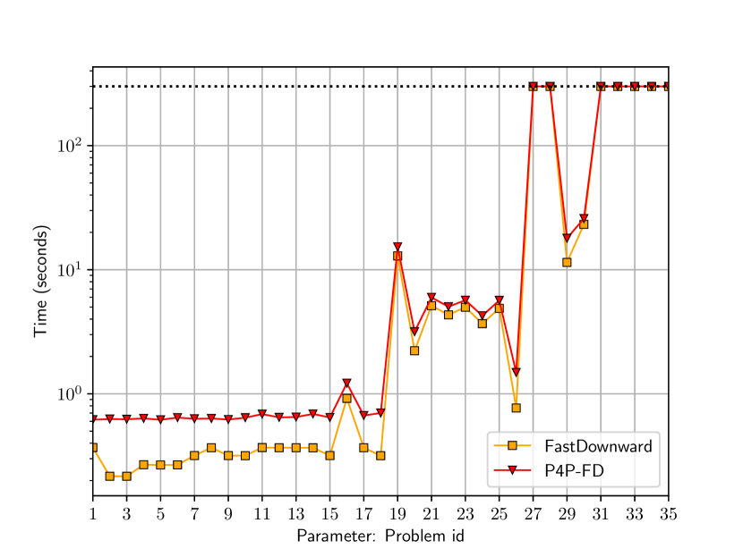
(a) BlocksWorld deterministic, experiment 1 (35 instances).

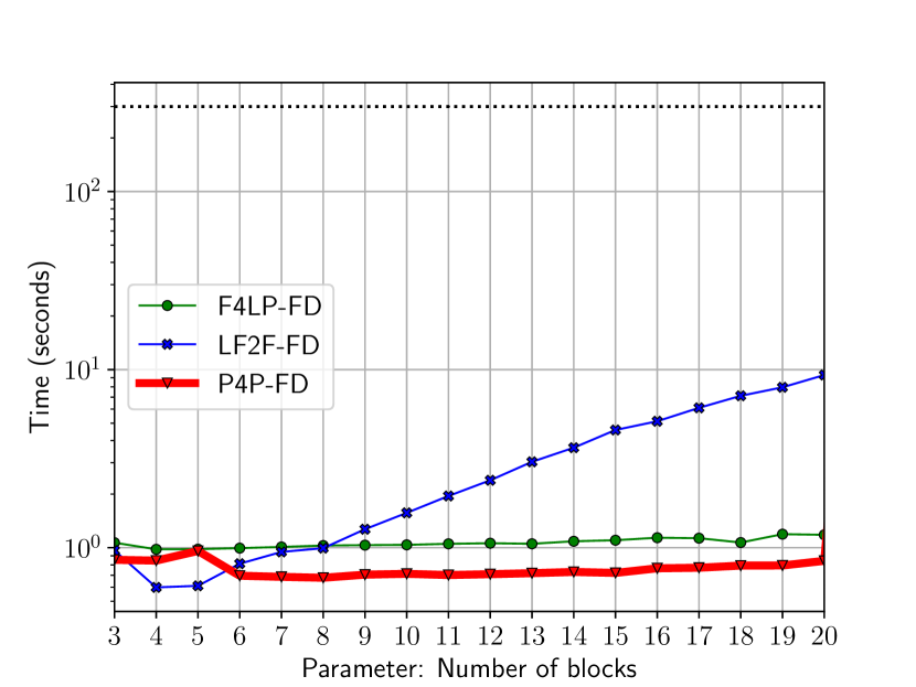
(b) BlocksWorld deterministic, experiment 2.

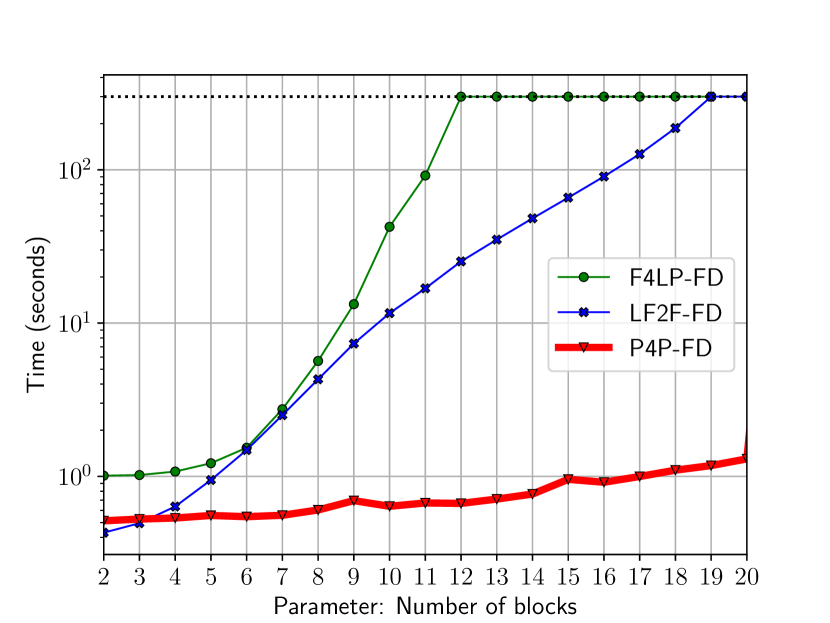
(c) BlocksWorld deterministic, experiment 2.

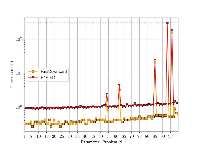
(d) Elevator, experiment 1 (100 instances)

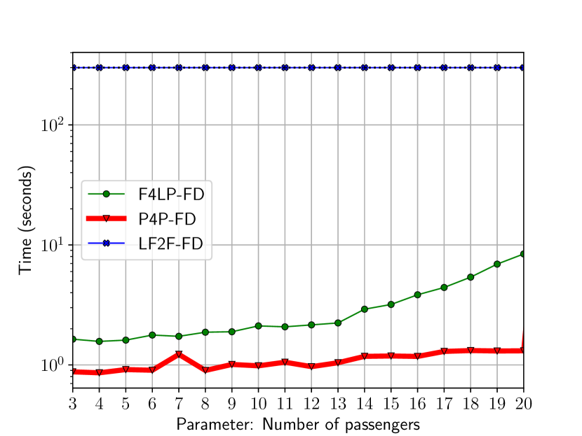
(e) Elevator, experiment 2.

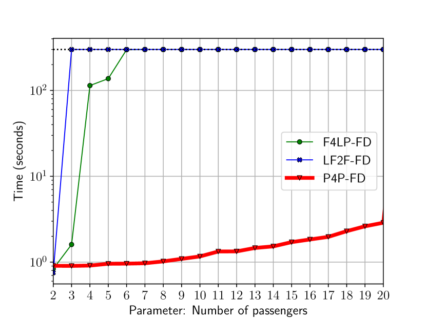
(f) Elevator, experiment 2.

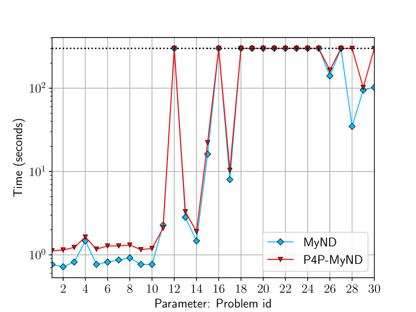
(g) BlocksWorldND, experiment 1.

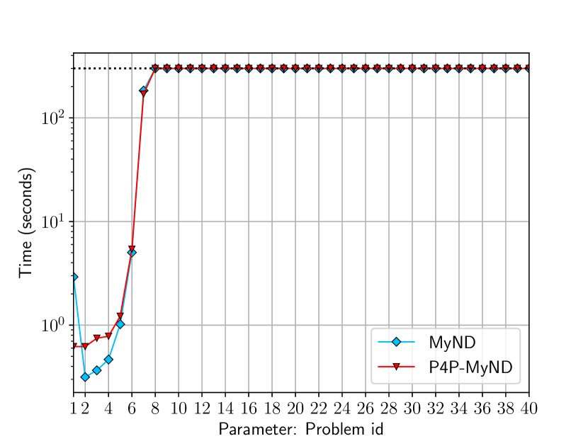
(h) TriangleTireworld, experiment 1.

Figure 1: Comparison results on all benchmarks.

Elevator

We run Experiment 1 over the 150 problems available from the planning competition. Figure 1(d) shows the running time of $\mathsf{FD}$ versus $\mathsf{{\mathsf{P4P}}+{\mathsf{FD}}}$, where we observe that we get a similar result as in BlocksWorld (deterministic). Regarding experiments of type 2, we considered as size of the problem the number of passengers $n$, with $2n$ floors, all passengers starting from floor $0$ with destination for a passenger $i$ the floor $2i$. The goal formula is to serve all the passengers, i.e. $\varphi_{n}={\mathsf{O}}(served(p_{1}))\wedge\cdots{\mathsf{O}}(served(p_{n}))$. Its ltl_f counterpart is $\varphi^{f}_{n}={\mathsf{F}}(served(p_{1}))\wedge\cdots{\mathsf{F}}(served(p_{n}))$. For Experiment 2, we fixed the formula parameter $n=3$ and increased the number of passengers from $3$ to $20$. The results are shown in Figure 1(e). For Experiment 2, we increased the parameter $n$ from $3$ to $20$, and the results are in Figure 1(f). In the former case, we note that the size of the problem does not affect the performances of our tool $\mathsf{{\mathsf{P4P}}+{\mathsf{FD}}}$, instead of what happens for $\mathsf{{\mathsf{F4LP}}+{\mathsf{FD}}}$ and $\mathsf{{{\mathsf{LF2F}}+{\mathsf{FD}}}}$; and in the latter case, our tool largely outperforms its competitors, which timeout far earlier. In fact, the planner $\mathsf{{{\mathsf{LF2F}}+{\mathsf{FD}}}}$ gets stuck in the translation step, and we conjecture it is due to the high bookkeeping machinery introduced to produce the compiled domain and problem.

BlocksWorld (nondeterministic)

The experimental setup is very similar to the deterministic case with the same goal description, except that the problems are taken from a different planning competition. In Figure 1(g), we show the results for the experiment 1, run over 30 problems. We note that, also in the nondeterministic case, the overhead is quite small wrt the running time of the original task. We also run the experiments of type 2 and 2, and we observed that our tool, backed by $\mathsf{MyND}$, scales much better than $\mathsf{{\mathsf{LF2F}}+{\mathsf{MyND}}}$, and it is competitive with $\mathsf{{{\mathsf{F4LP}}+{\mathsf{MyND}}}}$, and sometimes better (especially in 2). Due to lack of space, we do not report these results here, but they can be found in the supplementary material.

TriangleTireworld

We run experiment 1 over the 40 problem instances from the planning competition. The results are shown in Figure 1(h). We can see that the running time overhead is very small also in this case. Regarding experiments of type 2, we consider as size of the problem the length $n$ of a side of the triangle, and a spare tire in every location. The temporal goal is to visit $m$ locations in the following order: $l11,l12,l22,l23,\dots$. E.g. the past formula for $m=3$ is: $\varphi_{m}={\mathsf{O}}(vehicle\_at(l22)\wedge{\mathsf{Y}}({\mathsf{O}}(vehicle\_at(l21)\wedge{\mathsf{Y}}({\mathsf{O}}(vehicle\_at(l11))))))$. The fixed goal for experiment 2 is: ${\mathsf{O}}(vehicle\_at(l31)\wedge{\mathsf{Y}}({\mathsf{O}}(vehicle\_at(l21)\wedge{\mathsf{Y}}({\mathsf{O}}(vehicle\_at(l12))))))$. These domain and goals turned out to be tough for all the approaches under study, with few solved instances. These results can be found in the supplementary material.

Discussion

These experiments show that in virtually all cases our tool performs significantly better than its competitors, in both the deterministic and nondeterministic case. We attribute this to the rather different nature of our approach and the competitors’ approach: whilst $\mathsf{F4LP}$ and $\mathsf{LTLFOND2FOND}$ compute the explicit dfa of the goal formula (whose size is worst-case doubly-exponential for ltl_f and worst-case exponential for ppltl wrt the size of the formula) and then compile it into the new domain and problem, the compilation of our tool processes the formula directly generating only a minimal number of additional fluents, and uses them to delegate the semantic evaluation of the ppltl goal to the planner. Another important point is that our technique does not introduce auxiliary actions, hence allowing the planner to work more efficiently in searching for a solution. This is confirmed by the fact that in the experiments the number of expanded nodes is often the same of the original task, whereas for the other tools that is not the case.

7 Discussion

Our research shows that ppltl is a sweet spot in expressing temporally extended goals since it only introduces minimal overhead. Handling ppltl is particularly simple and elegant. A single compilation that works for deterministic and nondeterministic planning domains (and, in fact, it also works for MDPs, but this is out of the scope of the paper). Section 4 gives the mathematics behind it; Section 5 gives an implementation directly based on the mathematics (for this elegance we need derived predicates); Section 6 shows the practical effectiveness of the approach.

These nice results hold for ppltl only. Indeed, (1) it is crucial to work with a dfa in order not to introduce forms of decision that would impact planning (crucial in nondeterministic domains). (2) iterated progression can be thought of as an implicit form of dfa construction (every formula has a single progression), meaning that the iterated progression must be able to create doubly-exponentially-many non-equivalent annotations to be complete in the case of ltl_f, whereas only exponentially-many (the truth-value of linearly many new fluents) for ppltl. Even if we do not use automata explicitly, the connection with automata remains important in understanding how to deal with ltl_f/ppltl because it gives the essential information needed in order to be able to check if a trace satisfies an ltl_f/ppltl formula.

Specifically, ppltl translates into an exponential dfa, while ltl_f translates into an exponential nfa. If we consider a deterministic domain, with both dfa and nfa we can do the Cartesian product with the domain on-the-fly while searching for the solution (PSPACE). For FOND, we first need to compute the nfa and then transform it into a dfa on-the-fly (2EXPTIME). Instead, ppltl remains EXPTIME.

Although not always crisply stated, these observations are at the base of much of the related research.

Bacchus et al. [1997] does something very similar to us. The similarity comes from the fact that both approaches are based on progression (i.e. regression) of ppltl, i.e. on the “fixpoint equivalences” based on “now” and “next” (“previously”), see e.g. the survey [Emerson, 1990]. In fact, we can use our Section 4 to formally justify the correctness of the approach in that paper (where correctness is not proved). Also, our translation could be used to implement their decision tree based transitions and rewards. This is something to investigate in future works related to non-Markovian Decision Processes.

Sohrabi et al. [2011] uses ppltl for $\phi_{expl}$. However, (cf. p. 265, col. 2), they handle them in a naïve way, in view of recent understanding [De Giacomo et al., 2020]. They consider ppltl formulas as ltl_f formulas on the reverse trace (const), compute the nfa for the ltl_f (exp), reverse it (poly), so the trace is in the correct direction, build the planning domain and solve the problem (PSPACE). The resulting technique is worst-case EXPSPACE, whereas it could be PSPACE. Moreover, they do not exploit the fact that one can obtain the dfa of the reverse language in single exponential [De Giacomo et al., 2020] and on-the-fly while planning (this paper).

Mallett et al. [2021] considers a probabilistic variant of ltl_f (without the past). Their construction is based on progression. Since the progression is deterministic, it needs to mimic a dfa to be complete. Given that the minimal dfa corresponding to an ltl_f formula may contain doubly-exponential states in the worst-case, correspondingly the iterated progression needs to create doubly-exponential non-equivalent formulas to be complete. Additionally, here we cannot use nfas because they would interfere with probabilities. It would be interesting to use ppltl instead of ltl_f, since this would simplify their algorithmic part.

Bienvenu et al. [2011] introduces a very advanced language to talk about preferences based on ltl_f. The setting is on deterministic domains, so planning with this basic component remains PSPACE. Progression can be effectively used (as witnessed by TLPlan). However, as discussed above, iterated progression can explode in the worst-case, being deterministic, and hence does not take advantage of the fact that for this problem the nfa would suffice, see Camacho et al. [2017], Camacho & McIlraith [2019].

Zhu et al. [2019], (cf. Sec. 4), studies ppltl and uses it to solve ltl_f through mso. Note that if we use fol/mso to express temporal properties on finite traces, moving from properties as pure-past to pure-future (and vice versa) is poly (though checking fol/mso temporal properties is non-elementary). Unfortunately, if we use ppltl/ltl_f, although they have the same expressive power and the same expressive power of fol in expressing temporal properties on finite traces, moving from one to the other is in 3EXPTIME (matching lower bound is unknown).

We should note that bad complexity results on translations to dfas are not always mirrored as reduced performance of the systems. This is actually not often the case, e.g., the best ltl_f to dfa translators are first based on the translation to fol (poly) and then use fol in MONA [Henriksen et al., 1995] to obtain the dfa (non-elementary). However, the simplicity and elegance of ppltl treatment stand out.

We close the section by observing that ppltl has a special role in the ltl literature. For instance, the Manna & Pnueli [1990]’s temporal hierarchy is based on ppltl “atoms” $\alpha$ that are in the context of very simple future ltl formulas: Safety, G $\alpha$; Co-Safety F $\alpha$; Liveness GF $\alpha$; Persistence FG $\alpha$; and so on. Also, an important result is the separation of temporal formulas with both past and future into a boolean combination of pure-future and pure-past formulas [Gabbay et al., 1994]. Finally, recent proposals of an ltl fragment with both future and past operators are of interest. These new fragments, with atoms of arbitrary ppltl formulas within the scope of future operators, behave well on synthesis (related to planning) [Cimatti et al., 2020].

8 Conclusion

In this paper, we have studied planning for temporally extended goals expressed in ppltl. ppltl is particularly interesting for expressing goals since it allows to express sophisticated tasks as in the Formal Methods literature, while the worst-case computational complexity of Planning in both deterministic and nondeterministic domains (FOND) remains the same as for classical reachability goals. Note that, this is not the case for planning in nondeterministic domains for ltl_f goals, even though ppltl and ltl_f share the same formal expressiveness [De Giacomo et al., 2020].

We exploit this nice feature of ppltl to devise a direct technique for translating planning for ppltl goals into planning for standard reachability goals with only a minimal overhead. Experiments confirm the effectiveness of such a technique in practice. As a result, our technique enables state-of-the-art tools for classical, FOND strong and FOND strong-cyclic planning to handle ppltl goals seamlessly, essentially maintaining the performances they have for classical reachability goals.

In this paper, we have focused on ppltl. How to extend our results to goals given in ppldl, which is a strictly more expressive variant of ppltl [De Giacomo et al., 2020], remains for further studies.

References

- van der Aalst et al. [2009] van der Aalst, W., Pesic, M., & Schonenberg, H. (2009). Declarative Workflows: Balancing Between Flexibility and Support. Computer Science - R&D, 23, 99–113.
- Alechina et al. [2018] Alechina, N., Logan, B., & Dastani, M. (2018). Modeling norm specification and verification in multiagent systems. FLAP, 5.
- Aminof et al. [2020] Aminof, B., De Giacomo, G., & Rubin, S. (2020). Stochastic fairness and language-theoretic fairness in planning in nondeterministic domains. In ICAPS (pp. 20–28). AAAI Press.
- Bacchus et al. [1996] Bacchus, F., Boutilier, C., & Grove, A. (1996). Rewarding behaviors. In AAAI (pp. 1160–1167).
- Bacchus et al. [1997] Bacchus, F., Boutilier, C., & Grove, A. (1997). Structured solution methods for non-markovian decision processes. In AAAI (pp. 112–117). Citeseer.
- Bacchus & Kabanza [1998] Bacchus, F., & Kabanza, F. (1998). Planning for temporally extended goals. Ann. Math. Artif. Intell., 22, 5–27.
- Bacchus & Kabanza [2000] Bacchus, F., & Kabanza, F. (2000). Using temporal logics to express search control knowledge for planning. Artif. Intell., 116, 123–191.
- Baier et al. [2008a] Baier, C., Katoen, J.-P., & Guldstrand Larsen, K. (2008a). Principles of Model Checking.
- Baier et al. [2008b] Baier, J. A., Fritz, C., Bienvenu, M., & McIlraith, S. A. (2008b). Beyond classical planning: Procedural control knowledge and preferences in state-of-the-art planners. In AAAI (pp. 1509–1512). AAAI.
- Baier & McIlraith [2006a] Baier, J. A., & McIlraith, S. A. (2006a). Planning with first-order temporally extended goals using heuristic search. In AAAI (pp. 788–795). AAAI.
- Baier & McIlraith [2006b] Baier, J. A., & McIlraith, S. A. (2006b). Planning with temporally extended goals using heuristic search. In ICAPS (pp. 342–345). AAAI.
- Bienvenu et al. [2011] Bienvenu, M., Fritz, C., & McIlraith, S. A. (2011). Specifying and computing preferred plans. Artificial Intelligence, 175, 1308–1345.
- Borgwardt et al. [2022] Borgwardt, S., Hoffmann, J., Kovtunova, A., Krötzsch, M., Nebel, B., & Steinmetz, M. (2022). Expressivity of planning with horn description logic ontologies (technical report). In AAAI.
- Brafman & De Giacomo [2019a] Brafman, R. I., & De Giacomo, G. (2019a). Planning for LTLf/LDLf goals in non-markovian fully observable nondeterministic domains. In IJCAI (pp. 1602–1608). ijcai.org.
- Brafman & De Giacomo [2019b] Brafman, R. I., & De Giacomo, G. (2019b). Regular decision processes: A model for non-markovian domains. In IJCAI (pp. 5516–5522). ijcai.org.
- Brafman et al. [2018] Brafman, R. I., De Giacomo, G., & Patrizi, F. (2018). LTLf/LDLf non-markovian rewards. In AAAI (pp. 1771–1778). AAAI Press.
- Bryce & Buffet [2008] Bryce, D., & Buffet, O. (2008). 6th international planning competition: Uncertainty part. IPC’08, .
- Bylander [1994] Bylander, T. (1994). The computational complexity of propositional strips planning. Artif. Intell., 69, 165–204.
- Camacho et al. [2018] Camacho, A., Baier, J. A., Muise, C. J., & McIlraith, S. A. (2018). Finite LTL synthesis as planning. In ICAPS (pp. 29–38). AAAI Press.
- Camacho et al. [2019a] Camacho, A., Bienvenu, M., & McIlraith, S. A. (2019a). Towards a unified view of ai planning and reactive synthesis. In ICAPS (pp. 58–67). volume 29.
- Camacho & McIlraith [2019] Camacho, A., & McIlraith, S. A. (2019). Strong fully observable non-deterministic planning with ltl and ltl-f goals. In IJCAI (pp. 5523–5531).
- Camacho et al. [2019b] Camacho, A., Toro Icarte, R., Klassen, T. Q., Valenzano, R. A., & McIlraith, S. A. (2019b). LTL and beyond: Formal languages for reward function specification in reinforcement learning. In IJCAI (pp. 6065–6073). ijcai.org.
- Camacho et al. [2017] Camacho, A., Triantafillou, E., Muise, C. J., Baier, J. A., & McIlraith, S. A. (2017). Non-deterministic planning with temporally extended goals: LTL over finite and infinite traces. In AAAI (pp. 3716–3724). AAAI Press.
- Chandra et al. [1981] Chandra, A., Kozen, D., & Stockmeyer, L. (1981). Alternation. J. of the ACM, 28.
- Cimatti et al. [2020] Cimatti, A., Geatti, L., Gigante, N., Montanari, A., & Tonetta, S. (2020). Reactive synthesis from extended bounded response LTL specifications. In FMCAD (pp. 83–92). IEEE.
- Cimatti et al. [1997] Cimatti, A., Giunchiglia, F., Giunchiglia, E., & Traverso, P. (1997). Planning via model checking: A decision procedure for AR. In ECP (pp. 130–142). Springer volume 1348 of Lect. Notes Comput. Sci..
- Cimatti et al. [2003] Cimatti, A., Pistore, M., Roveri, M., & Traverso, P. (2003). Weak, strong, and strong cyclic planning via symbolic model checking. Artif. Intell., 147, 35–84.
- Cimatti et al. [1998] Cimatti, A., Roveri, M., & Traverso, P. (1998). Strong planning in non-deterministic domains via model checking. In AIPS (pp. 36–43). AAAI.
- De Giacomo et al. [2014] De Giacomo, G., De Masellis, R., & Montali, M. (2014). Reasoning on ltl on finite traces: Insensitivity to infiniteness. In AAAI. volume 28.
- De Giacomo et al. [2020] De Giacomo, G., Di Stasio, A., Fuggitti, F., & Rubin, S. (2020). Pure-past linear temporal and dynamic logic on finite traces. In IJCAI. volume 20.
- De Giacomo & Fuggitti [2021] De Giacomo, G., & Fuggitti, F. (2021). Fond4ltlf: Fond planning for ltlf/pltlf goals as a service. In ICAPS, demo track.
- De Giacomo et al. [2019] De Giacomo, G., Iocchi, L., Favorito, M., & Patrizi, F. (2019). Foundations for restraining bolts: Reinforcement learning with LTLf/LDLf restraining specifications. In ICAPS (pp. 128–136). AAAI Press.
- De Giacomo & Rubin [2018] De Giacomo, G., & Rubin, S. (2018). Automata-theoretic foundations of FOND planning for ltlf and ldlf goals. In IJCAI (pp. 4729–4735).
- De Giacomo & Vardi [2013] De Giacomo, G., & Vardi, M. (2013). Linear temporal logic and linear dynamic logic on finite traces. In IJCAI.
- De Giacomo & Vardi [2015] De Giacomo, G., & Vardi, M. (2015). Synthesis for LTL and LDL on finite traces. In IJCAI.
- De Giacomo & Vardi [1999] De Giacomo, G., & Vardi, M. Y. (1999). Automata-theoretic approach to planning for temporally extended goals. In ECP (pp. 226–238). Springer volume 1809 of Lect. Notes Comput. Sci..
- Emerson [1990] Emerson, E. A. (1990). Temporal and modal logic. In Handbook of Theoretical Computer Science, Volume B: Formal Models and Sematics.
- Fisher & Wooldridge [2005] Fisher, M., & Wooldridge, M. (2005). Temporal reasoning in agent-based systems. In H. of Temporal Reasoning in AI.
- Gabaldon [2011] Gabaldon, A. (2011). Non-Markovian control in the situation calculus. Artif. Intell., 175, 25–48.
- Gabbay et al. [1994] Gabbay, D. M., Hodkinson, I., & Reynolds, M. (1994). Temporal logic: mathematical foundations and computational aspects.
- Geffner & Bonet [2013] Geffner, H., & Bonet, B. (2013). A Concise Introduction to Models and Methods for Automated Planning.
- Gerevini et al. [2009] Gerevini, A., Haslum, P., Long, D., Saetti, A., & Dimopoulos, Y. (2009). Deterministic planning in the fifth international planning competition: PDDL3 and experimental evaluation of the planners. Artif. Intell., 173, 619–668.
- Giunchiglia & Traverso [1999] Giunchiglia, F., & Traverso, P. (1999). Planning as model checking. In ECP. volume 1809 of Lect. Notes Comput. Sci..
- Helmert [2006] Helmert, M. (2006). The fast downward planning system. J. Artif. Int. Res., 26, 191–246.
- Henriksen et al. [1995] Henriksen, J., Jensen, J., Jørgensen, M., Klarlund, N., Paige, B., Rauhe, T., & Sandholm, A. (1995). Mona: Monadic second-order logic in practice. In Tools and Algorithms for the Construction and Analysis of Systems, First International Workshop, TACAS ’95, LNCS 1019.
- Hoffmann & Edelkamp [2005] Hoffmann, J., & Edelkamp, S. (2005). The deterministic part of IPC-4: An overview. J. Artif. Int. Res., 24, 519–579.
- Knobbout et al. [2016] Knobbout, M., Dastani, M., & Meyer, J. (2016). A dynamic logic of norm change. In ECAI.
- Lichtenstein et al. [1985] Lichtenstein, O., Pnueli, A., & Zuck, L. D. (1985). The glory of the past. In Logic of Programs (pp. 196–218). Springer volume 193 of Lect. Notes Comput. Sci..
- Mallett et al. [2021] Mallett, I., Thiébaux, S., & Trevizan, F. (2021). Progression heuristics for planning with probabilistic ltl constraints. In AAAI (pp. 11870–11879). volume 35.
- Manna & Pnueli [1990] Manna, Z., & Pnueli, A. (1990). A hierarchy of temporal properties. In PODC (pp. 377–410). ACM.
- Mattmüller et al. [2010] Mattmüller, R., Ortlieb, M., Helmert, M., & Bercher, P. (2010). Pattern database heuristics for fully observable nondeterministic planning. ICAPS, 20, 105–112.
- McDermott et al. [1998] McDermott, D., Ghallab, M., Howe, A., Knoblock, C., Ram, A., Veloso, M., Weld, D., & Wilkins, D. (1998). PDDL – the planning domain definition language. Technical Report ICAPS.
- Muise et al. [2012] Muise, C., McIlraith, S., & Beck, C. (2012). Improved non-deterministic planning by exploiting state relevance. In ICAPS. volume 22.
- Pistore & Traverso [2001] Pistore, M., & Traverso, P. (2001). Planning as model checking for extended goals in non-deterministic domains. In IJCAI (pp. 479–486). Morgan Kaufmann.
- Rintanen [2004] Rintanen, J. (2004). Complexity of planning with partial observability. In ICAPS (pp. 345–354).
- Sohrabi et al. [2011] Sohrabi, S., Baier, J., & McIlraith, S. (2011). Preferred explanations: Theory and generation via planning. In AAAI (pp. 261–267). volume 25.
- Thiébaux et al. [2005] Thiébaux, S., Hoffmann, J., & Nebel, B. (2005). In defense of pddl axioms. Artificial Intelligence, 168, 38–69.
- Torres & Baier [2015] Torres, J., & Baier, J. A. (2015). Polynomial-time reformulations of LTL temporally extended goals into final-state goals. In ICAPS.
- Zhu et al. [2019] Zhu, S., Pu, G., & Vardi, M. Y. (2019). First-order vs. second-order encodings for ltlf-to-automata translation. In TAMC (pp. 684–705).