Domain Invariant Model with Graph Convolutional Network for Mammogram Classification

Abstract

Due to its safety-critical property, the image-based diagnosis is desired to achieve robustness on out-of-distribution (OOD) samples. A natural way towards this goal is capturing only clinically disease-related features, which is composed of macroscopic attributes (e.g., margins, shapes) and microscopic image-based features (e.g., textures) of lesion-related areas. However, such disease-related features are often interweaved with data-dependent (but disease irrelevant) biases during learning, disabling the OOD generalization. To resolve this problem, we propose a novel framework, namely Domain Invariant Model with Graph Convolutional Network (DIM-GCN), which only exploits invariant disease-related features from multiple domains. Specifically, we first propose a Bayesian network, which explicitly decomposes the latent variables into disease-related and other disease-irrelevant parts that are provable to be disentangled from each other. Guided by this, we reformulate the objective function based on Variational Auto-Encoder, in which the encoder in each domain has two branches: the domain-independent and -dependent ones, which respectively encode disease-related and -irrelevant features. To better capture the macroscopic features, we leverage the observed clinical attributes as a goal for reconstruction, via Graph Convolutional Network (GCN). Finally, we only implement the disease-related features for prediction. The effectiveness and utility of our method are demonstrated by the superior OOD generalization performance over others on mammogram benign/malignant diagnosis.

Methodology	test on InH1		test on InH2
	train on InH2 +InH3 +DDSM	train on InH1	train on InH1 +InH3 +DDSM	train on InH2
ERM [10]	0.822	0.888	0.758	0.847
Ours	0.948	0.952	0.874	0.898
Methodology	test on InH3		test on DDSM
	train on InH1 +InH2 +DDSM	train on InH3	train on InH1 +InH2 +InH3	train on DDSM
ERM [10]	0.735	0.776	0.779	0.847
Ours	0.858	0.864	0.892	0.919

TABLE I: AUC evaluation under out-of-distribution (OOD) and the same distribution (in-distribution). ERM defines training by Empirical Risk Minimization. For each testing set, the results on the left are under OOD circumstance, and the results on the right are under the same distribution.

I Introduction

In medical diagnosis, a realistic issue that may hamper the clinical practice is: the distribution of data can vary greatly across healthcare facilities (e.g., hospitals), due to inconsistent imaging and preprocessing methods such as staining and scanning. This can fail the traditional Empirical Risk Minimization (ERM), as ERM heavily relies on independent and identically distributed (i.i.d) assumption and can exploit spurious correlation during the data-fitting process. Such a spurious correlation may not generalize on unseen domains. This can be manifested by nearly 9% AUC drop of ERM, as shown in Tab. I. To satisfy the high safety requirements for medical diagnosis, it is desired to develop a model that can generalize well on out-of-distribution samples (i.e., distribute differently with training samples).

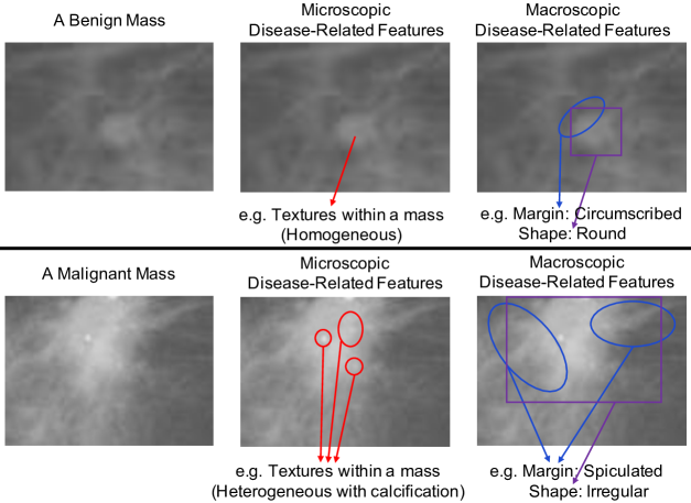
Figure 1: The macroscopic and microscopic features of benign/malignant masses. The features behave differently between benign and malignant masses. Microscopic features are homogeneous for benign and heterogeneous for malignant (red arrow). For macroscopic features, the margin is clear and circumscribed in benign mass while spiculated in malignant mass (blue arrow). The shape is regular (e.g., round) in benign mass while irregular in malignant mass (purple arrow).

Recently, there is increasing attention for OOD generalization, such as [1, 9, 18]. Given data from multiple domains, the above methods are proposed to learn the invariant representations for prediction. Such invariant learning can improve the generalization ability on general tasks. However, these methods fail to incorporate the medical priors about disease-related features and the underlying generating processes of them, which can limit the utility in medical diagnosis.

In clinical diagnosis, the disease-related features that doctors often employ for prediction are mainly composed of two parts: macroscopic and microscopic features. Specifically, the macroscopic features encode morphology-related attributes [22] of lesion areas, as summarized in American College of Radiology (ACR) [20]; the microscopic features, which reflect subtle patterns of lesions, are hard to observe but helpful for classifying the disease. Taking the mammogram in Fig. 1 as an illustration, the macroscopic features, e.g., can refer to the margins, shapes, spiculations of the masses; while the microscopic features, e.g., can refer to the textures, and the curvatures of contours [7]. As these disease-related features can expose abnormalities (e.g., irregular shapes or textures) for malignancy compared to benign ones, they are determined by the disease status and provide invariant evidence for diagnosis. However, they are often mixed with other domain-dependent but disease-irrelevant noise, such as imaging and preprocessing biases, making them difficult to be identified during learning.

We encapsulate these priors into a latent generative model in Fig. 2, in which the latent variables are explicitly split into three parts: the macroscopic features $a$, the microscopic features $s$ and other disease irrelevant features $z$. These three parts are modeled differently, such that i) as disease-related features, the $a$ and $s$ are invariantly related to the disease label, with $a$ additionally generating the observed attributes; while ii) other disease-irrelevant features $z$ are domain-dependent. We then prove that the disease-related features can be disentangled from others. Under this guarantee, we propose a disentangling learning framework, dubbed as Domain Invariant Model with Graph Convolutional Network (DIM-GCN), to only exploit disease-related features for prediction. Specifically, we design two-branch encoders for each domain: Relevant Enc that is shared by all domains to learn disease-related features, and a domain-specific Irrelevant Enc to extract disease-irrelevant features. To impose the disentanglement of invariant diseased-related features, among all latent features that participate in the reconstruction of the image, we only use the disease-related features for disease prediction. To additionally capture the macroscopic features, we enforce them to reconstruct the clinical attributes via Graph Convolutional Network (GCN).

To verify the utility and effectiveness of domain generalization, we perform our method on mammogram mass benign/malignant classification. Here the clinical attributes are those related to the masses, which are summarized in ACR [20] and easy to obtain. We consider four datasets (one public and three in-house) that are collected from different sources. In each time’s evaluation, we train our method on three datasets and test on the remaining one. The results show that our method can outperform others by 6.2%. Besides, our learned disease-related features can successfully encode the information on the lesion areas.

As a summary, our contributions are mainly three-fold:

1. We propose a novel generative model, which incorporates medical priors regarding disease-related features;

2. We propose a novel DIM-GCN that can disentangle the disease-related features from others to prompt medical diagnosis on an unseen domain;

3. Our model can achieve state-of-the-art OOD generalization performance for mass benign/malignant diagnosis.

II Related Work

Patch-Level Mammogram Mass Classification. Previous approaches that can be used to address patch-level mammogram mass benign/malignant classification without ROI annotations are roughly categorized into three classes: (i) the GAN-based methods, e.g., Li et al. [19]; (ii) the disentangling-based methods, e.g., Guided-VAE [8]; (iii) the attribute-guided methods, e.g., Chen et al. [6], ICADx [13]. For class (i), they propose an adversarial generation to augment training data for better prediction. However, lacking the guidance of medical knowledge descents their performance. For class (ii), the disentangling mechanism can provide better disease-related representation learning but lacking the guidance of the prior of attributes limits their performance. For class (iii), the prior of attributes is considered into their methods. Insufficient utilization of attributes descents their effectiveness. Besides, above all methods do not consider domain bias while training. Changing the domain of data will directly cause drops on their results. Motivated by the above, we use the disentangling mechanism and domain knowledge with Graph Convolutional Network(GCN) for better learning invariant disease-related features and improving the ability of generalization in unseen domains.

Domain Generalization. Domain generalization considers multiple domains and aims to improve the generalization performance in an unseen domain. For domain generalization, previous methods will lead to a dramatic performance decrease when testing on data from a different distribution with a different bias [11]. Thus such previous models are not robust enough to the actual task [2]. Progress has been made on domain generalization which can be roughly divided into three classes: (i) Learning the domain-specific constraints, e.g., [5] aims to learn domain-specific masks to characterize different domains(e.g., clipart, sketch, and painting). They fail in medical images for masks are not suitable to distinguish different domains. (ii) Disentangle-based, e.g., [11] proposes a generative model with three independent latent subspaces for the domain, the class and the residual variations respectively. They did not make use of the medical attribute knowledge which is important in our mammogram classification. (iii) Design invariant constrains, e.g., [1] aims to learn invariant representation across environments by minimizing the Invariant Risk Minimization term. [9] and [18] use adversarial way with the former performs domain-adversarial training to ensure a closer match between the source and the target distributions and the latter trains an Adversarial Autoencoder. Lack of disentanglement and the guidance of medical prior knowledge limits their performance on generalization.

III Methodology

Problem Setup $\&$ Notations. Denote $x\in\mathcal{X},y\in\mathcal{Y},A\in\mathcal{A}$ respectively as the image, benign/malignant label, and clinical attributes (e.g., margins, lobulations). We collect datasets $\{x^{d}_{i},y^{d}_{i},A^{d}_{i}\}$ from multiple domains (i.e., healthcare facilities in our scenario) $d\in\mathcal{D}$. Our goal is learning a disease-prediction model $f:\mathcal{X}\to\mathcal{Y}$ from training domains $\mathcal{D}_{\mathrm{train}}$, that generalizes well on all domains $\mathcal{D}\supset\mathcal{D}_{\mathrm{train}}$, especially out-of-distribution domains $\mathcal{D}_{\mathrm{test}}:=\mathcal{D}\setminus\mathcal{D}_{\mathrm{train}}$. Denote $m:=|\mathcal{D}_{\mathrm{train}}|$.

This section is organized as follows: in Sec. III-A, we first introduce our Bayesian network that encodes the medical prior knowledge of our problem. We prove that the disease-related features can be disentangled from others. With this theoretical guarantee, we in Sec. III-B introduce our learning method dubbed as Domain Invariant Model with Graph Convolutional Network. Specifically, we reformulate the Variational Auto-Encoder (VAE) in Sec. III-B1; then, we introduce our inference (encoder) model with disentanglement learning and generative (decoder) model with GCN in Sec. III-B2; finally, we introduce a variance regularizer to further prompt the learning of invariant disease-related features in Sec. III-B3.

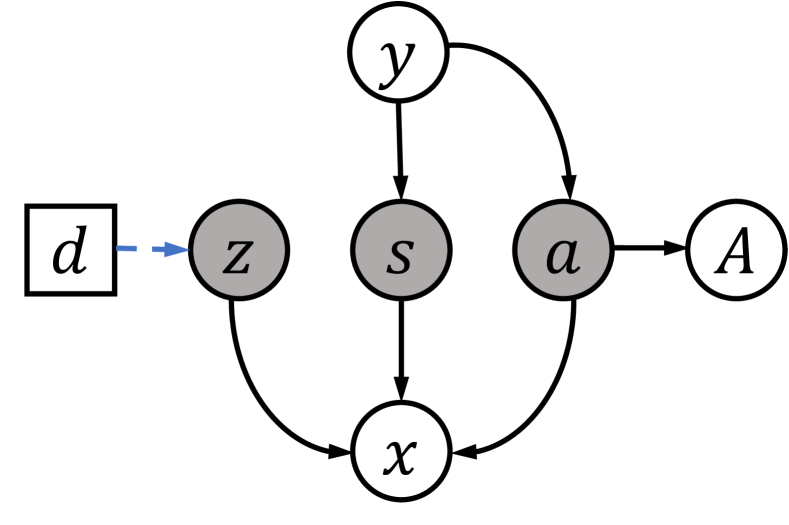
Figure 2: Our Bayesian Network. The Bayesian network depicts the underlying generation process of the medical disease. The edges represent the probabilistic relationships between images, attributes, disease labels and domains in our problem.

III-A Bayesian Network with Latent Variables

Our Bayesian Network is illustrated in Fig. 2, which encodes the medical priors of disease diagnosis into the generating processes. Specifically, among all latent components that generate the image $x$, we split them into three parts: $a$, $s$ and $z$ that respectively encodes the information of macroscopic (such as shapes, margins [20]), microscopic (textures, curvatures of contours [7]) and disease-irrelevant features. As disease-related features that provide stable evidence for diagnosis, the $a$ and $s$ are assumed to generate from the disease status $y$ via an invariant mechanism ($p(s,a|y)$ is invariant across domains). Such features are often mixed with other variations, a.k.a. $z$, which encodes the domain-dependent information such as imaging and pre-processing biases. This mixture can lead to the difficulty of identifying the $s,a$ for prediction. To further differentiate $a$ from $s$, we additionally assume that the $a$ generates the clinical attributes $A$, which are often employed by clinicians for prediction due to its explainability and easiness to observe. Such disease-related macroscopic attributes $A$ are objectively existing properties of the lesion area. These properties and their corresponding lesion area, are generated concurrently from the disease status $y$, via the latent component $a$ [4]. Our Fig. 2 depicts the underlying generation process of the medical image and clinical attributes, instead of the disease inference process on the observational data. The microscopic features $s$, which is hard to observe, can provide additional information for prediction. We assume the generating processes from $a\to A$ and $z,s,a\to X$, as they follow from physical laws, to be invariant across domains [21].

A natural identifiability question towards robust prediction imposes: will the disease-related features (that estimated from $x$) can be possibly identified, without mixing the information of others? The following theorem provides a positive answer, which provides a guarantee for us to propose the learning method that can learn the $p^{d}(x,y,A)$ well.

Theorem III.1 (Informal).

Suppose that multiple environments are diverse enough, then there exist functions $h_{s},h_{z},h_{a}$ such that, for any latent variables $(\tilde{s},\tilde{a},\tilde{z})$ and $(s^{\star},a^{\star},z^{\star})$ giving rise to the same observational distribution (i.e., $p(x,y,A)$), we have that the

$$\tilde{s}=h_{s}(s^{\star}),\ \tilde{z}=h_{z}(z^{\star}),\ \tilde{a}=h_{a}(a^{\star}).$$

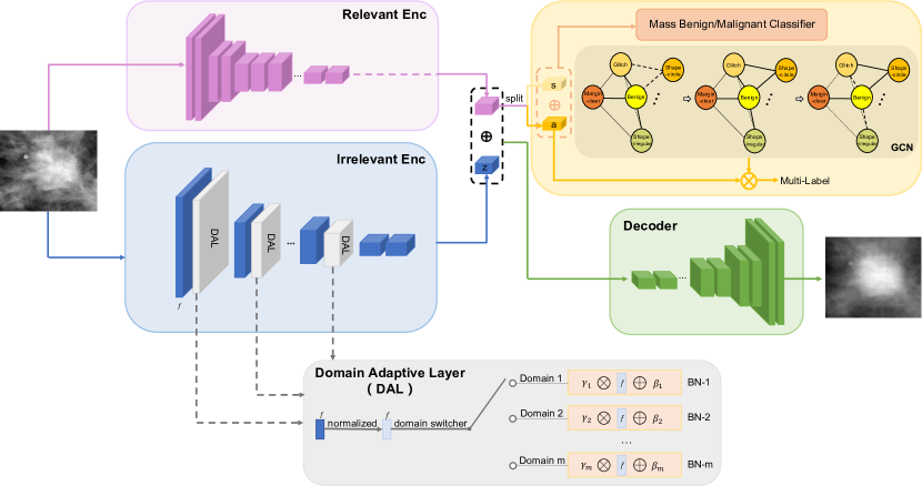
Figure 3: Domain Invariant Model with Graph Convolutional Network (DIM-GCN). In the training phase, the input image is fed into Relevant Enc and Irrelevant Enc. In Irrelevant Enc, images from different domains are fed into corresponding domain adaptive layer respectively. We optimize the overall network on multiple training domains. In the test phase, an image from an unseen domain is only fed into Relevant Enc to get the disease-related factors $s$ and $a$. The final prediction result is obtained by the classifier.

Remark 1.

It can be easily seen from Theorem III.1 that if $(s^{\star},a^{\star},z^{\star})$ denote the ground-truth latent variables that generate $p(x,y,A)$, then the learned latent variables $\tilde{s}$, $\tilde{a}$ and $\tilde{z}$ do not mix information of others. The diversity condition, which requires that the extent of dependency of $y$ on $z$ varies across domains, is almost necessary to ensure the invariance disease-related features to be identified, and is thus similarly assumed in the literature [21].

III-B Domain Invariant Model with Graph Convolutional Neural Network

Guided by Theorem III.1, to achieve disentanglement, it is sufficient to learn $\{p^{d}(x,y,A)\}$ well. To achieve this goal, we first reformulate the Evidence Lower BOund (ELBO) of VAE based on Fig. 2 in Sec. III-B1, followed by inference (a.k.a Encoder) and generative (a.k.a Decoder) models in Sec. III-B2 and finally the variance regularizer in Sec. III-B3.

III-B1 ELBO Reformulation

The VAE [14] was proposed to learn $p(x)$ with $Z\to X$. To resolve the intractability for high-dimensional data $x$, it introduced the variational distribution $q(z|x)$ and to maximize the Evidence Lower BOund (ELBO) defined as $\max_{q,p_{\theta}}\mathbb{E}_{p(x)}\left(\mathbb{E}_{q(z|x)}\left(\log{\frac{p_{\theta}(x,z)}{q(z|x)}}\right)\right)\leq\mathbb{E}_{p(x)}\left(\log{p_{\theta}(x)}\right)$. The “=” can be achieved as long as $q(z|x)=p_{\theta}(z|x)$. In other words, the variational distribution can learn the behavior of the posterior distribution during optimization.

To learn $p^{d}(x,y,A)$ following from Fig. 2 for each domain $d$, we similarly derive the ELBO for

$$\log p_{\theta}^{d}(x,y,A) =\log p_{\theta}^{d}(x)+\log p_{\theta}^{d}(A|x)+\log p_{\theta}^{d}(y|x,A),$$

according to the Bayesian formula. We introduce the variational distribution $q^{d}(v|x)$ ($v:=(z,s,a)$). The corresponding ELBO for the first term, i.e., $\log p^{d}_{\theta}(x)$ can be derived as:

$$\mathbb{E}_{p^{d}(x,y,A)}\left(\mathbb{E}_{q^{d}(v|x)}\left(\log{\frac{p^{d}_{\theta}(x,v)}{q^{d}(v|x)}}\right)\right)$$ (1)

$$= \mathbb{E}_{p^{d}(x,y,A)}\left(\mathbb{E}_{q^{d}(v|x)}\left(\log{p_{\theta}(x|v)}\right)\right)$$

$$\ \ \ \ \ -\mathbb{E}_{p^{d}(x,y,A)}\left(\mathrm{KL}(q^{d}(v|x),p_{\theta}^{d}(v))\right),$$

which is $\leq\mathbb{E}_{p^{d}(x,y,A)}\left(\log{p^{d}_{\theta}(x)}\right)$ and the equality can only be achieved once $q^{d}(v|x)=p_{\theta}^{d}(v|x)$. Combined with $\log p^{d}_{\theta}(A|x)$ and $\log p^{d}_{\theta}(y|x,A)$, the loss function for domain $d$ is:

$$\ \ell^{d}(q^{d},p_{\theta}^{d})=-\frac{1}{n_{d}}\sum_{i=1}^{n_{d}}\left(\log p^{d}_{\theta}(A_{i}|x_{i})+\log p^{d}_{\theta}(y_{i}|x_{i},A_{i})+\right.$$

$$\ \ \ \ \ \ \left.\mathbb{E}_{q^{d}(v|x_{i})}\left(\log{p_{\theta}(x_{i}|v)}\right)-\mathrm{KL}(q^{d}(v|x_{i}),p_{\theta}^{d}(v))\right).$$

With $q^{d}(v|x)$ learned to approximate $p^{d}_{\theta}(v|x)$, the $p^{d}_{\theta}(A|x)$ and $p^{d}_{\theta}(y|x,A)$ can be approximated via:

$$p^{d}_{\theta}(A|x) \approx\int p_{\theta}(A|a)q(a|x)da,$$ (2)

$$p^{d}_{\theta}(y|A,x) \approx\int p_{\theta}(y|s,a)q(s,a|x)dads.$$ (3)

The $p_{\theta}(x|v)$ in Eq. (1) and $p_{\theta}(A|a)$, $p_{\theta}(y|s,a)=p_{\theta}(s,a|y)p_{\theta}(y)/p_{\theta}(s,a)$ in Eq. (2), (3), which are invariant across domains, have their parameters $\theta$ shared by all domains $d$. To optimize the loss, we need to respectively parameterize the prior models $p^{d}_{\theta}(z,s,a)$, inference models $q^{d}(z,s,a|x)$ and generative models $p_{\theta}(x|z,s,a),p_{\theta}(A|a),p_{\theta}(y|s,a)$.

Following the graph in Fig. 2, the $p_{\theta}^{d}(z,s,a)$ can be factorized as $p_{\theta}^{d}(z,s,a)=p(s,a)p_{\theta}(z|d)$, where the $p(s,a)$ can be modeled as isotropic Gaussian while $p_{\theta}(z|d)$ can be learned via Multilayer Perceptron (MLP) with one-hot encoded vector $d\in\mathbb{R}^{m}$ as input.

Inference models. We adopt the mean-field approximation to factorize $q(z,s,a|x,d)$ as $q(s,a|x)*q(z|x,d)$. This motivates us to implement a two-branch encoder, a domain-invariant (a.k.a, relevant encoder) one $q(s,a|x)$ and a domain-specific one $q(z|x,d)$ (a.k.a, irrelevant encoder), as shown in Fig. 3 and the subsequent section. Together with prior models, the inference models are the inputs of KL-divergence term.

Generative models. We optimize to reconstruct $x,A$ and predict $y$ via $p_{\theta}(x|z,s,a),p_{\theta}(A|a)$ and $p_{\theta}(y|s,a)$. Particularly, to model the correlation among attributes, we implement Graph Convolutional Network (GCN) to learn $p_{\theta}(A|a)$.

As illustrated in Fig. 3, all models are optimized following a variational Auto-Encoder scheme. In the next subsection, we will introduce the architectures of the encoder, decoder to implement the inference models and the generative models.

III-B2 Encoder-Decoder Architecture

As shown in Fig. 3, our DIM-GCN contains the following components: two-branch encoders dubbed as Relevant Enc for $q(s,a|x)$ and Irrelevant Enc for $q(z|x,d)$ to respectively encode the disease-related (i.e., $s,a$) and -irrelevant features (i.e., $z$), a decoder for $p_{\theta}(x|v)$ to reconstruct the image $x$, a GCN for $p_{\theta}(A|a)$ to reconstruct the attributes, and finally a disease classifier for $p_{\theta}(y|s,a)$ for final disease classification. Each component is introduced in details below.

Two-Branch Encoders for $q(s,a|x)$ and $q^{d}(z|x)$. Motivated by the factorization of $q^{d}(z,s,a|x)$ into $q(s,a|x)*q(z|x,d)$ in Sec. III-A, we propose two-branch encoders, namely Relevant Enc for $q(s,a|x)$ and Irrelevant Enc for $q(z|x,d)$. For the disease classification $p(y|s,a)$, the Relevant Enc encodes the disease-related features $(s,a)$ from $x$, with the macroscopic features $a$ additionally enforced to reconstruct the attributes $A$ well. The Irrelevant Enc encodes other disease-irrelevant features $z$ from $x$. As such features are domain-specific, we incorporate a domain adaptive layer into the encoder. Specifically, the domain adaptive layer that following the convolutional layer contains m batch normalization (BN) layers, as shown in Fig. 3. The scaling and shifting parameters in each BN are learned adaptively with the domain in the training.

Denote the features from the convolutional layer as $f$, then we get the output features of the domain adaptive layer for each domain $d$ ($d\in\{1,...,m\}$) by:

$$f_{1}=BN_{\gamma_{1},\beta_{1}}(f) =\gamma_{1}*\hat{f}+\beta_{1}$$ (4)

$$\vdots$$

$$f_{m}=BN_{\gamma_{m},\beta_{m}}(f) =\gamma_{m}*\hat{f}+\beta_{m}$$

with $\hat{f}=\frac{f-\mu_{B}}{\sqrt{\delta_{B}^{2}+\epsilon}}$ is the normalized features by the mini-batch mean $\mu_{B}$ and variance $\delta_{B}$. Each domain has a set of learning parameters $\gamma_{d},\beta_{d}$.

Such a two-branch encoder is trained by a KL-divergence term:

$$\mathbb{E}_{p^{d}(x)}\left(\mathrm{KL}(q^{d}(z,s,a|x),p^{d}(z,s,a)\right)$$

$$\approx \frac{1}{n_{d}}\sum_{n}\left(\mathrm{KL}(q(s,a|x_{n}),p(s,a))\right.$$

$$\ \ \ \left.+\mathrm{KL}(q(z|x_{n},d)),p(z|d))\right)\overset{\Delta}{=}\mathcal{L}_{\mathrm{kl}}^{d},$$ (5)

with prior models $p(s,a)$ modeled as isotropic Gaussian and $p(z|d)$ as a two-layer MLP that takes the word embedding of $d\in\mathbb{R}^{m}$ as input.

The disentanglement of $z,s,a$ lies in their asymmetric roles in the generating processes. Specifically, among all latent variables $z,s,a$ that reconstructs $x$ via decoder for $p_{\theta}(x|z,s,a)$, only $s,a$ are used in the classifier for $p_{\theta}(y|s,a)$ and only $a$ is used in GCN for $p_{\theta}(A|a)$ to reconstruct attributes $A$.

Decoder for $p_{\theta}(x|z,s,a)$. The decoder, that outputs $\hat{x}:=\mathrm{Dec}(z,s,a)$, is trained to reconstruct the original image $x$ well by minimizing

$$\mathbb{E}_{p^{d}(x)}\left(\mathbb{E}_{q^{d}(v|x)}(\log{p_{\theta}(x|v)})\right)$$ (6)

$$\approx \frac{1}{n_{d}}\sum_{n}\|x_{n}-\hat{x}_{n}\|_{2}^{2}\overset{\Delta}{=}\mathcal{L}_{\mathrm{rec}}^{d}.$$

Graph Convolutional Network for $p_{\theta}(A|a)$. The correlations between attributes in lesions are strongly related and helpful to the cancer diagnosis. To make full use of this prior knowledge and further promote the disentanglement of the invariant disease-related features, we parameterize $p_{\theta}(A|a)$ by a Graph Convolutional Network (GCN) which is a flexible way to capture the topological structure in the label space.

Along with [6], we build a graph $G=(U,E)$ with twelve nodes and consider each attribute as a node, e.g., Shape-circle, Margin-clear. Each node $u\in U$ represents the word embedding of the attributes. Each edge $e\in E$ represents the inter-relevance between attributes. The inputs of the graph are features representations $H^{l}$ and corresponding correlation matrix $B$ which is calculated in the same as [6]. For the first layer, $H^{0}\in{\mathbb{R}}^{c\times c^{\prime}}$ denotes the one-hot embedding matrix of each attribute node where $c$ is the number of attributes, $c^{\prime}$ is the length of embeddings. Then, the feature representation of the graph at every layer [15] can be calculated as follow:

$$H^{l+1}=\delta(BH^{l}W^{l}),$$ (7)

where $\delta(\cdot)$ is LeakyRelu, $W^{l}$ is the transformation matrix which is the parameter to be learned in the $l$th layer. The output $\{\hat{g}^{k}\}_{k}$ (with $\hat{g}^{k}:=\mathrm{GCN}([\text{Relevant-Enc}(x)]_{\mathcal{A}})$) is learned to approximate attributes $\{g^{k}\}_{k}$ (with each $g^{k}\in\{0,1\}$) to train the GCN:

$$-\mathbb{E}_{p^{d}(A|x)}\left(\log{p_{\theta}(A|x)}\right)$$ (8)

$$\approx -\frac{1}{n_{d}}\sum_{n}\left(\sum_{k=1}^{C}g_{n}^{k}\log\hat{g}_{n}^{k}+(1-g_{n}^{k})\log(1-\hat{g}_{n}^{k})\right)\overset{\Delta}{=}\mathcal{L}_{\mathrm{gcn}}^{d}.$$

Disease Classifier for $p_{\theta}(y|s,a)$. Finally, the classification network for $p_{\theta}(y|s,a)$ is trained via

$$-\mathbb{E}_{p^{d}(A|x)}\left(\log{p_{\theta}(y|A,x)}\right)$$ (9)

$$\approx -\frac{1}{n_{d}}\sum_{n}\left(y_{n}\log\hat{y}_{n}+(1-y_{n})\log(1-\hat{y}_{n})\right)\overset{\Delta}{=}\mathcal{L}_{\mathrm{cls}}^{d},$$ (10)

where $\hat{y}:=\mathrm{Cls}(\text{Relevant-Enc}(x))$ is the predicted label for $y$. Combined with Eq. (5), (6), (8), (9), the loss for domain $d$ is:

$$\mathcal{L}^{d}=\mathcal{L}_{\mathrm{kl}}^{d}+\mathcal{L}_{\mathrm{rec}}^{d}+\mathcal{L}^{d}_{\mathrm{gcn}}+\mathcal{L}_{\mathrm{cls}}^{d}.$$ (11)

III-B3 Variance Regularizer

To further prompt the invariance for encoded $s,a$ across multiple domains, we leverage an additional variance regularizer [16],

$$\mathcal{L}_{\mathrm{var}}=\underset{d}{Var}\{\mathcal{L}^{d}_{\mathrm{gcn}}\}+\underset{d}{Var}\{\mathcal{L}^{d}_{\mathrm{cls}}\},$$ (12)

where $\underset{d}{Var}\{\mathcal{L}^{d}_{\mathrm{gcn}}\}$ and $\underset{d}{Var}\{\mathcal{L}^{d}_{\mathrm{cls}}\}$ respectively denotes the variance of $\mathcal{L}^{d}_{\mathrm{gcn}}$ and $\mathcal{L}^{d}_{\mathrm{cls}}$ across $\mathcal{D}_{\mathrm{train}}$. This is motivated by our expectation to learn $s,a$ that can stably predict disease and reconstruct the clinical attributes. Combined with the loss for domain $d$ in Eq. (11), the final loss is

$$\mathcal{L}=\sum_{d}\mathcal{L}^{d}+\beta\mathcal{L}_{\mathrm{var}}$$ (13)

where $\beta>0$ trades off the losses and the variance regularizer.

IV Experiments

Datasets. To evaluate the effectiveness of our model, we apply our model on patch-level mammogram mass benign/malignant classification, which drives increasing attention recently [23, 17] due to its clinical use. We consider both the public dataset DDSM [3] and three in-house datasets: InH1, InH2 and InH3. These datasets are collected from different hospitals with different types of imaging devices (e.g., X-ray devices). For each dataset, the region of interests (ROIs) (malignant/benign masses) are cropped based on the annotations of radiologists the same as [13]. For each dataset, we randomly split it into training, validation, and testing sets with 8:1:1 patient-wise ratio. The training/valid/testing samples we use contain 1165 ROIs from 571 patients/143 ROIs from 68 patients/147 ROIs from 75 patients in DDSM [3], 684 ROIs from 292 patients/87 ROIs from 38 patients/83 ROIs from 33 patients in InH1, 840 ROIs from 410 patients/104 ROIs from 50 patients/105 ROIs from 52 patients in InH2, and 565 ROIs from 271 patients/70 ROIs from 33 patients/70 ROIs from 34 patients in InH3.

Implementation Details. For a fair comparison, all methods are conducted under the same setting and share the same encoder backbone, i.e., ResNet34 [10]. Meanwhile, the decoder is the deconvolution network of the encoder. For attribute annotations, in DDSM [3] annotations can be parsed from the ”.OVERLAY” file. The third line in the ”.OVERLAY” file has annotations for types, shapes, and margins of masses. And in our in-house datasets, we obtain attribute annotations from the verify of one director doctor based on the annotations of three senior doctors. The inputs are resized into 224 × 224 with random horizontal flips and fed into networks. We implement all models with PyTorch. We implement Adam for optimization. The weight hyperparameter in variance regularizer $\beta$ is 1 in our experiments. The clinical attributes contain circle, oval, irregular, circumscribed, obscured, ill-defined, is-lobulated, not-lobulated, is-spiculated, not-spiculated. We add additional benign and malignant nodes to learn the correlation between the combination of attributes and benign/malignant. To verify the effectiveness of domain generalization, we test on all four datasets under OOD settings, i.e., every dataset is used as the testing set respectively while the other three are used as the training sets. To remove the randomness, we run for 10 times and report the average value of them. To further validate our effectiveness, we also give in-distribution results of each dataset which can be seen as the upper bounds of each dataset, i.e., using the training set with the same domain as the testing set. For a fair comparison, the number of above all training sets all keep the same. Area Under the Curve (AUC) is used as the evaluation metric in image-wise. For implementation of compared baselines, we directly load the published codes of ERM [10], Chen et al. [6], DANN [9], MMD-AAE [18], DIVA [11], IRM [1] and Prithvijit et al.[5] during test; while we re-implement methods of Guided-VAE [8], ICADx [13] and Li et al. [19] for lacking published source codes.

Methodology	train on InH2 +InH3 +DDSM	train on InH1 +InH3 +DDSM	train on InH1 +InH2 +DDSM	train on InH1 +InH2 +InH3
	test on InH1	test on InH2	test on InH3	test on DDSM
ERM [10]	0.822	0.758	0.735	0.779
Chen et al. [6]	0.877	0.827	0.804	0.830
Guided-VAE [8]	0.872	0.811	0.779	0.811
ICADx [13]	0.882	0.802	0.777	0.826
Li et al. [19]	0.848	0.794	0.769	0.815
DANN [9]	0.857	0.811	0.781	0.813
MMD-AAE [18]	0.860	0.783	0.770	0.786
DIVA [11]	0.865	0.809	0.784	0.813
IRM [1]	0.889	0.830	0.795	0.829
Prithvijit et al.[5]	0.851	0.796	0.772	0.797
Ours	0.948	0.874	0.858	0.892

TABLE II: AUC evaluation of Domain Generalization on public DDSM [3] and three in-house datasets. (OOD settings: training and testing are from different domains)

IV-A Results

Compared Baselines. We compare our model with following methods: a) ERM [10] directly trains the classifier via ResNet34 by Empirical Risk Minimization; b) Chen et al. [6] achieves multi-label classification with GCN for attributes prediction; c) Guided-VAE [8] also implements disentangle network but lacks the medical prior knowledge of attributes during learning; d) Li et al. [19] improve performance by generating more benign/malignant images via adversarial training; e) ICADx [13] also proposes the adversarial learning method but additionally introduces shape/margins information for reconstruction; f) DANN [9] uses adversarial way to ensure a closer match between the source and the target distributions; g) MMD-AAE [18] extends adversarial autoencoders by imposing the Maximum Mean Discrepancy (MMD) measure; h) DIVA [11] proposes a generative model with three independent latent subspaces; i) IRM [1] designs Invariant Risk Minimization term to learn invariant representation across environments; j) Prithvijit et al.[5] add domain specific masks learning for better domain generalization.

Methodology	train on InH1	train on InH2	train on InH3	train on DDSM [3]
	test on InH1	test on InH2	test on InH3	test on DDSM [3]
ERM [10]	0.888	0.847	0.776	0.847
Chen et al. [6]	0.924	0.878	0.827	0.871
Guided-VAE [8]	0.921	0.867	0.809	0.869
ICADx [13]	0.911	0.871	0.816	0.879
Li et al. [19]	0.908	0.859	0.828	0.875
Ours-single	0.952	0.898	0.864	0.919

TABLE III: In-distribution AUC results on public DDSM [3] and three in-house datasets (training and testing on the same single dataset.)

Irrelevant Encoder	Attribute Learning	$s$	$\mathcal{L}_{rec}$	Var	AUC(InH1)	AUC(InH2)	AUC(InH3)	AUC(DDSM)
$\times$	$\times$	$\times$	$\times$	$\times$	0.822	0.758	0.735	0.779
$\times$	$\times$	$\times$	$\times$	$\checkmark$	0.829	0.768	0.746	0.788
$\times$	multi-task	$\times$	$\times$	$\times$	0.851	0.793	0.775	0.801
$\times$	$\mathcal{L}_{gcn}$	$\times$	$\times$	$\times$	0.877	0.827	0.804	0.830
$\times$	$\mathcal{L}_{gcn}$	$\times$	$\times$	$\checkmark$	0.884	0.835	0.808	0.835
$\times$	$\mathcal{L}_{gcn}$	$\times$	$\checkmark$	$\times$	0.911	0.846	0.816	0.844
DAL	$\mathcal{L}_{gcn}$	$\times$	$\checkmark$	$\times$	0.931	0.862	0.841	0.878
DAL	$\times$	$\times$	$\checkmark$	$\times$	0.913	0.840	0.823	0.852
$\times$	$\mathcal{L}_{gcn}$	$\checkmark$	$\checkmark$	$\times$	0.916	0.851	0.821	0.859
one branch	$\mathcal{L}_{gcn}$	$\checkmark$	$\checkmark$	$\times$	0.926	0.856	0.830	0.863
DAL	$\mathcal{L}_{gcn}$	$\checkmark$	$\checkmark$	$\times$	0.941	0.867	0.849	0.887
DAL	$\mathcal{L}_{gcn}$	$\checkmark$	$\checkmark$	$\checkmark$	0.948	0.874	0.858	0.892

TABLE IV: Ablation Studies Testing on InH1/InH2/InH3/DDSM [3] while Training on the Other Three Datasets. (OOD settings)

train on InH(1,2)	train on InH(1,3)	train on InH(3,2)	train on InH(1,2,3)
0.885	0.881	0.887	0.892

TABLE V: Ablation study on the combination of training data sets. Take testing on pubilic dataset DDSM [3] as an example. (OOD settings)

test on InH1	test on InH2	test on InH3	test on DDSM [3]
0.939	0.874	0.852	0.892

TABLE VI: AUC of testing on data set InH1/InH2/InH3/DDSM [3] while training on InH1+InH2+InH3.

Results & Analysis on Domain Generalization. To verify the effectiveness of our learning method on out-of-distribution (OOD) samples, we train our model on the combination of three datasets from three different hospitals and test on the other unseen dataset from the other hospital which is the different domain from all training sets.

As shown in Table II, our methods can achieve state-of-the-art results in all settings. Specifically, the first five lines are the methods based on different representation learning and we extend them to our domain generalization task. The next five lines are the methods aiming at domain generalization. Li et al. [19] generate more data under the current domain, the larger number of data improves the performance compared with ERM [10] but the augmentation for the current domain greatly limits its ability of domain generalization. Prithvijit et al.[5] learn domain-specific mask (Clipart, Sketch, Painting), however, the gap exists in medical images can not balance through mask learning. DANN [9] and MMD-AAE [18] design distance constraints between the source and the target distributions. However, the key to achieving great classification performance in medical diagnosis is to explore the disease-related features which are invariant in multiple domains. Simply distance-constrain is not robust enough and limits the performance. The advantage of Guided-VAE [8] and DIVA [11] over mentioned methods above may be due to the disentanglement learning in the former methods. IRM [1] learns invariant representation across environments by Invariant Risk Minimization term which improves their results to a certain extent. However, lacking the guidance of attribute and disentanglement learning limits their performance. Guided-VAE [8] introduces the attribute prediction which improves their performance than DIVA [11]. The improvements in ICADx [13], Guided-VAE [8] prove the importance of the guidance of attribute learning. Although ICADx [13] uses the attributes during learning, it fails to model correlations between attributes and benign/malignant diagnosis, which limits their performance. With further exploration of attributes via GCN, our method can outperform ICADx [13], Guided-VAE [8]. Compared to Chen et al. [6] that also implement GCN to learn attributes, we additionally employ disentanglement learning with variance regularizer which can help to identify invariant disease-related features during prediction.

Comparison with In-distribution results. In addition, to further validate our effectiveness, we compute the in-distribution AUC performance of every single dataset. We implement the methods which aim at representation learning on each single dataset, i.e., training and testing on the data from the same hospital(domain). Such in-distribution results can serve as the upper bounds of our generalization method since their training and testing data come from the same domain distribution. To adapt our proposed mechanism to the in-distribution situation, we change our network with two branches to only one branch accordingly for extracting features into $a,s,z$ since training data is only from one hospital(Ours-single), i.e., one domain without domain influence. As shown in Table III, based on disentanglement mechanism and the guidance of attribute learning, Ours-single still get the state-of-art performance. We argue that the disentangling mechanism with the guidance of attributes helps effective learning of disease-related features under a single domain. Results in Table III can be seen as the upper bound results of each setting in Table II. Our results in Table II are slightly lower than results in Table III by 0.4% to 2.7%. We argue that based on our mechanism for domain generalization, our method training under OOD can get the evenly matched effect with the training mode of the in-distribution that training and testing on the same domain. For example, as shown when testing on DDSM [3], performances of our model training on InH1+InH2+InH3 and training on DDSM itself are comparable.

IV-B Ablation Study

Ablation study on each components. To verify the effectiveness of each component in our model, we evaluate some variant models. Table IV shows the ablation study results (under OOD settings: testing on InH1/InH2/InH3/DDSM respectively, training on the other three datasets).

Here are some interpretations for the variants:

1. Irrelevant Encoder denotes whether using irrelevant encoder during the reconstructing phase, with One branch denotes only using one branch for the irrelevant encoder without distinguishing multiple domains and DAL denotes using domain adaptive layer for distinguishing multiple domains in irrelevant encoder;

2. Attribute Learning denotes the way to use attributes: $\times$ means not using any attributes for learning, multi-task means using a fully connected layer to predict the multiple attributes, and $\mathcal{L}_{gcn}$ means using our GCN network for learning attributes;

3. $s$ denotes whether split the latent factor $s$ out for disentanglement in training;

4. $\mathcal{L}_{rec}$ denotes whether use the reconstruction loss in training;

5. $Var$ denotes whether use the Variance Regularizer in training.

ratio of ADL	train on InH2 +InH3 +DDSM	train on InH1 +InH3 +DDSM	train on InH1 +InH2 +DDSM	train on InH1 +InH2 +InH3
	test on InH1	test on InH2	test on InH3	test on DDSM
one layer	0.926	0.857	0.835	0.864
1/3	0.930	0.863	0.842	0.871
1/2	0.942	0.871	0.847	0.883
2/3	0.946	0.874	0.853	0.889
all	0.948	0.874	0.858	0.892

TABLE VII: Effectiveness of the ratio of domain adaptive layers on public DDSM [3] and three in-house datasets.

Methodology	train on InH2 +InH3 +DDSM	train on InH1 +InH3 +DDSM	train on InH1 +InH2 +DDSM	train on InH1 +InH2 +InH3
	test on InH1	test on InH2	test on InH3	test on DDSM
ME	0.946	0.873	0.855	0.891
GL	0.947	0.872	0.854	0.887
DAL	0.948	0.874	0.858	0.892

TABLE VIII: AUC evaluation of Domain Generalization on public DDSM [3] and three in-house datasets under different domain adaptive mechanisms.

As shown, every component is effective for classification performance. It is worth noting that using naive GCN also leads to a boosting of around 6% in average. Such a result can demonstrate that the attributes can guide the learning of disease-related features. Meanwhile, disentanglement learning also causes a noticeable promotion, which may be due to that the disease-related features can be easier identified through disentanglement learning without mixing information with others. Moreover, Line7-8 in Table IV validate disease-related features can be disentangled better with the guidance of exploring attributes. Line 2-3 from the bottom in Table IV validates that distinguishing multiple domains improves the generalization performance. Comparing the last two lines, the regularizer we used is also helpful to disentangle invariant disease-related features. Besides Line2, 5 and 12 of Table IV show that GCN and other components in our model are still well effective under variance constraints.

To abate the impact of the combination of training domains, we train our model under different training combinations. Take testing on DDSM [3] as an example. As shown in Table V, the more types of domains the better effect of our model. Due to the different correlations between different domains, the effect will be different under different combinations. But based on the inter mechanism of our model, influences between different domains are not obvious and three domains are sufficient to achieve comparable results.

Under the setting: testing on DDSM [3] (OOD) while training on InH1+InH2+InH3, we also list the results of our invariant model DIM-GCN (OOD model) under testing on the testing set of InH1/InH2/InH3 (in-distribution) as shown in Tab. VI. In addition, under the same setting, we also test our variant model Ours-single (in-distribution model). The result testing on unseen DDSM [3] (OOD) is 0.861, testing on InH1/InH2/InH3 (in-distribution) which are from the same training sets (InH1+InH2+InH3) are 0.944, 0.880, and 0.853 respectively. The variant model testing on InH1/InH2/InH3 (the same domain as the training set) behaves comparably with ours in Tab. VI and is slightly better since our DIM-GCN split some inter-domain correlation which can decent performance under domain generalization. Thus, the variant model faces a larger drop over our invariant model DIM-GCN when generalizing to the unseen DDSM dataset (0.892 vs 0.861).

Methodology	ACC -InH1	ACC -InH2	ACC -InH3	ACC -DDSM
ERM-multitask	0.618	0.560	0.596	0.662
Chen et al. [6]	0.827	0.795	0.748	0.842
ICADX [13]	0.743	0.647	0.612	0.739
Proposed Method	0.914	0.877	0.858	0.934

TABLE IX: Overall Prediction Accuracy of Multi Attributes (Mass shapes, Mass margins). Testing on InH1/InH2/InH3/DDSM [3] while Training on the Other Three Datasets. (OOD settings)

Ablation study on the ratio of using adaptive domain layers. To verify the effectiveness of the ratio of using adaptive domain layers, we replaced the original BN layer with DAL in different ratios in the Irrelevant Encoder. The results are shown in Tab. VII, specifically, $1/3$ means only $1/3$ BN layers in the network are replaced, others and so forth. As we can see, under the lower ratio, the performances are close to One branch in Tab. IV for poorer domain-interpretability. The higher ratio can get better performance with more robust domain-interpretability.

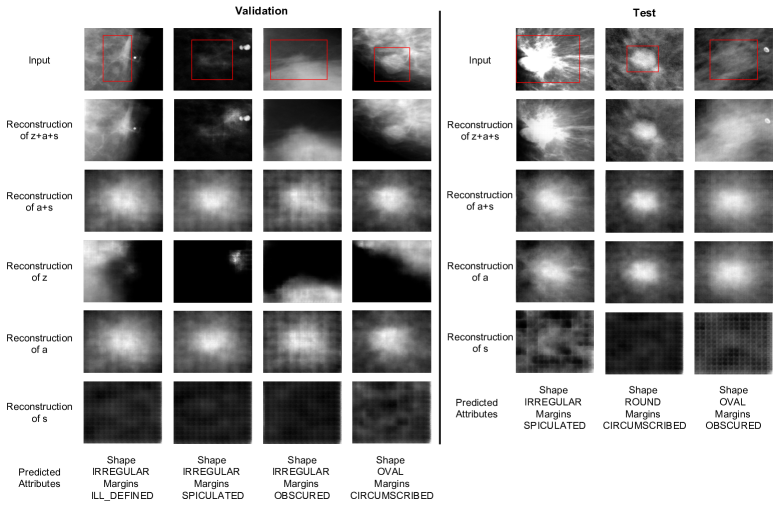
Figure 4: Visualization on validation and testing dataset under OOD settings. Lesion regions are marked by red rectangles. Each row represents the reconstruction of different latent variables. Each column represents different cases. Note that there is no reconstruction result of $z$ at the test stage because the test domain has no corresponding irrelevant encoder.

Ablation study on Domain Adaptive Mechanism To investigate the proposed adaptive domain layer in the Irrelevant Encoder sophisticatedly, we analyze various implementation forms of multiple domains as follows:

1. Multiple Encoders(ME). Since the irrelevant encoder contains the information of domain environments, an intuitive idea is using multiple irrelevant encoders so as to each domain has one irrelevant encoder directly.

2. Grouped Layer(GL). To reduce the parameter quantity of ME, we consider several groups of blocks with each group containing two blocks in the same structures. Each group only responds to one block each time, and different domains are different block combinations. The number of groups is set to $n$ that satisfies $2^{n}=m$ ($m$ denotes the number of domains, if $m$ is not the exponential power of 2, find $\hat{m}$ that is larger than $m$ and is the least number that satisfies $2^{n}=\hat{m}$). Thus each domain is a permutation combination based on each group choosing one block.

3. Domain Adaptive Layer(DAL). To further reduce the parameter quantity and achieve domain generalization, we propose the domain adaptive layer. For the batch normalization layers in the irrelevant encoder, each domain contains one specific batch normalization layer. The scaling and shifting parameters in each layer are learned adaptively.

We conduct experiments on the different implementation methods for modeling multiple domains. Results are shown in Table. VIII. Three different kinds of mechanisms have comparable performance. Since BN can usually be used as an effective measure for domain adaptation [12], DAL can be slightly better than the others with lighter computation, especially compared to ME.

IV-C Prediction Accuracy of Attributes

We argue that attributes can be the guidance of benign/malignant classification. In the current domain generalization task, we also calculate the OOD prediction accuracy of attributes in ours and other attribute-based representative methods in Table IX. The settings are: ACC-InH1: testing on InH1 while training on InH2+InH3+DDSM; ACC-InH2: testing on InH2 while training on InH1+InH3+DDSM; ACC-InH3: testing on InH3 while training on InH2+InH1+DDSM; ACC-DDSM [3]: testing on DDSM while training on InH2+InH3+InH1. Our method gets the best prediction accuracy on the attributes over other methods under OOD.

IV-D Visualization

We investigate the three latent factors $a$, $s$, and $z$ to see if our model is able to successfully disentangle them. We visualize different parts in Fig. 4 via the reconstruction effect and the predicted attributes of the current image. Since the Irrelevant Enc is partially domain-dependent, validating set is from the same domain as the training set but the testing set is from a different domain. We show reconstructions of all latent factors in validation (Left in Fig. 4) and reconstructions without $z$ in test (Right in Fig. 4). As we can see, the disease-related features $s+a$ mainly reflect the disease-related information since they mainly reconstruct the lesion regions without mixing others. The disease-irrelevant $z$ features mainly learn features such as the contour of the breasts, pectoralis, and other irrelevant glands without lesion information. It is worth noting that the white dots on the image which are caused by machine shooting are learned by $z$ as visualization. This means that through the ability of domain generalization our method can disentangle the irrelevant part successfully and prevent it from predicting the disease. Moreover, the macroscopic features $a$ capture the macroscopic attributes of the lesions, e.g., shape and density; while the microscopic features $s$ learn properties like global context, texture, or other invisible features but related to disease classification. These results further indicate the effectiveness and interpretability of our DIM-GCN.

V Conclusion

We propose a novel Domain Invariant Model with Graph Convolutional Network (DIM-GCN) on domain generalization for medical diagnosis, which is a multi-domain variational auto-encoder with the disentanglement mechanism equipped with a graph convolutional network. We evaluate our method on both public and in-house datasets for patch-level mammogram mass benign/malignant classification. Potential results demonstrate the effectiveness of our DIM-GCN, we will try to generalize this method to other medical imaging problems such as lung cancer, liver cancer, etc.

Appendix A Formal Description of Theorem 3.1

We assume that the $s,a|y$ and $z|d$ belong to the following exponential families:

$$p(z|d) :=p_{\mathbf{T}^{z},\bm{\Gamma}^{z}_{d}}(z|d),$$

$$p(s,a|y) :=p_{\mathbf{T}^{s},\bm{\Gamma}^{s}_{y}}(s|y)p_{\mathbf{T}^{a},\bm{\Gamma}^{a}_{y}}(a|y),$$

where

$$p_{\mathbf{T}^{u},\bm{\Gamma}^{u}_{o}}(u)={\small\prod_{i=1}^{q_{u}}}\exp\Big{(}{\small\sum_{j=1}^{k_{u}}}T^{u}_{i,j}(t_{i})\Gamma^{t}_{o,i,j}+B_{i}(u_{i})-C^{u}_{o,i}\Big{)},$$

for any $u\in\{s,a\}$ with $o=y$ and $u=z$ with $o=d$. The $\{T^{u}_{i,j}(u_{i})\}$, $\{\Gamma^{u}_{o,i,j}\}$ denote the sufficient statistics and natural parameters, $\{B_{i}\}$ and $\{C_{o,i}^{u}\}$ denote the base measures and normalizing constants to ensure the integral of distribution equals to 1. Let $\mathbf{T}^{u}(u)\!:=\![\mathbf{T}^{u}_{1}(u_{1}),...,\mathbf{T}^{u}_{q_{u}}(u_{q_{u}})]$ $\!\in\!\mathbb{R}^{k_{u}\times q_{u}}$ $\big{(}\mathbf{T}^{u}_{i}(u_{i})\!:=\![T^{u}_{i,1}(u_{i}),...,T^{u}_{i,k_{u}}(u_{i})],\forall i\in[q_{u}]\big{)}$, $\bm{\Gamma}^{u}_{o}\!:=\!\left[\bm{\Gamma}^{u}_{o,1},...,\bm{\Gamma}^{u}_{o,q_{u}}\right]$ $\!\in\!\mathbb{R}^{k_{u}\times q_{u}}$ $\big{(}\bm{\Gamma}^{u}_{o,i}\!:=\![\Gamma^{t}_{o,i,1},...,\Gamma^{t}_{o,i,k_{u}}],\forall i\in[q_{u}]\big{)}$. Further, we assume that the $s,a,z\to x$ and $a\to A$ follow the additive noise model (ANM):

$$x=f_{x}(s,a,z)+\epsilon_{x},A=f_{A}(a)+\epsilon_{A}.$$

Denote $\theta:=\{\mathbf{T}^{s},\mathbf{T}^{z},\mathbf{T}^{a},\bm{\Gamma}^{s}_{y},\bm{\Gamma}^{a}_{y},\bm{\Gamma}^{z}_{d},f_{x},f_{A}\}$, we define the disentanglement as follows:

Definition A.1.

We call the $s,a,z$ as disentangled under $\theta$, if for any $\tilde{\theta}:=\{\tilde{\mathbf{T}}^{s},\tilde{\mathbf{T}}^{z},\tilde{\mathbf{T}}^{a},\tilde{\bm{\Gamma}}^{s}_{y},\tilde{\bm{\Gamma}}^{a}_{y},\tilde{\bm{\Gamma}}^{z}_{d},\tilde{f}_{x},\tilde{f}_{A}\}$ that giving rise to the same observational distributions: $p_{\theta}(x,A,y|d)=p_{\tilde{\theta}}(x,A,y|d)$ for any $x,y,A$ and $d$, there exists invertible matrices $M_{s},M_{z},M_{a}$ and vectors $b_{z},b_{s},b_{a}$ such that:

$$\tilde{\mathbf{T}}([\tilde{f}_{x}^{-1}]_{\mathcal{S}}(x)) =M_{s}\mathbf{T}([f_{x}^{-1}]_{\mathcal{S}}(x))+b_{s},$$

$$\tilde{\mathbf{T}}([\tilde{f}_{x}^{-1}]_{\mathcal{Z}}(x)) =M_{z}\mathbf{T}([f_{x}^{-1}]_{\mathcal{Z}}(x))+b_{z},$$

$$\tilde{\mathbf{T}}([\tilde{f}_{x}^{-1}]_{\mathcal{A}}(x)) =M_{a}\mathbf{T}([f_{x}^{-1}]_{\mathcal{A}}(x))+b_{a},$$

where the $\mathcal{S},\mathcal{Z},\mathcal{A}$ denote the space of the latent variables $s,z,a$.

The theorem 3.1 is then mathematically formulated as:

Theorem A.2.

For any $\theta$, under following assumptions:

1. The characteristic functions of $\epsilon_{x},\epsilon_{A}$ are almost everywhere nonzero.

2. $f_{x},f_{A}$ are bijective;

3. The $\{T^{u}_{i,j}\}_{1\leq j\leq k_{u}}$ are linearly independent in $\mathcal{S}$, $\mathcal{Z}$ or $\mathcal{A}$ for each $i\in[q_{u}]$ for any $u=s,a,z$.

4. There exists $d_{1},...,d_{m}$ and $y_{1},...,y_{K}$ such that $\big{[}[\bm{\Gamma}^{z}_{d_{2}}-\bm{\Gamma}^{z}_{d_{1}}]^{\mathsf{T}},...,[\bm{\Gamma}^{z}_{d_{m}}-\bm{\Gamma}^{z}_{d_{1}}]^{\mathsf{T}}\big{]}^{\mathsf{T}}\in\mathbb{R}^{m\times(q_{z}\times k_{z})}$ and $\big{[}[\bm{\Gamma}^{u=s,a}_{y_{2}}-\bm{\Gamma}^{u=s,a}_{y_{1}}]^{\mathsf{T}},...,[\bm{\Gamma}^{u=s,a}_{y_{K}}-\bm{\Gamma}^{u=s,a}_{y_{1}}]^{\mathsf{T}}\big{]}^{\mathsf{T}}\in\mathbb{R}^{m\times(q_{u}\times k_{u})}$ have full column rank.

we have that $s,z,a$ are disentangled under $\theta$.

Proof.

For simplicity, we denote $\!\tilde{p}(u|o):=p_{\tilde{\mathbf{T}}^{u},\tilde{\bm{\Gamma}}^{u}_{o}}(u|o)$. Since $p_{\theta}(x|d,y)=p_{\tilde{\theta}}(x|d,y)$, then we have $\int p_{f_{x}}(x|s,a,z)p(s,a|y)p(z|d)dsdadz\!=\!\int p_{\tilde{f}_{x}}(x|s,a,z)\!\tilde{p}(s,a|y)\tilde{p}(z|d)dsdadz$. According to the chain rule of changing from $s,a,z$ to $\bar{x}\!:=\!f_{x}(s,a,z)$, we have that $\int p_{\varepsilon_{x}}(x-\bar{x})p(f_{x}^{-1}(\bar{x})|d,y)J_{f^{-1}}(\bar{x})d\bar{x}\!=\!\int p_{\varepsilon_{x}}(x-\bar{x})p(\tilde{f}_{x}^{-1}(\bar{x})|d,y)J_{\tilde{f}^{-1}}(\bar{x})d\bar{x}$, where $J_{f}(x)$ denotes the Jacobian matrix of $f$ on $x$. Denote $p^{\prime}(\bar{x}|d,y):=p(f_{x}^{-1}(\bar{x})|d,y)J_{f^{-1}}(\bar{x})$. Applying Fourier transformation to both sides, we have $F[p^{\prime}](\omega)\varphi_{\varepsilon_{x}}(\omega)=F[\tilde{p}^{\prime}](\omega)\varphi_{\varepsilon_{x}}(\omega)$, where $\varphi_{\varepsilon_{x}}$ denotes the characteristic function of $\varepsilon_{x}$. Since they are almost everywhere nonzero, we have that $F[p^{\prime}](\omega)=F[\tilde{p}^{\prime}]$, which means that $p^{\prime}(\bar{x}|d,y)=\tilde{p}^{\prime}(\bar{x}|d,y)$. This is equivalent to the following:

$$\log{\mathrm{vol}J_{f_{x}}(x)}+\sum_{u=s,a}\sum_{i=1}^{q_{u}}(\log{B_{i}([f_{x,i}^{-1}]_{\mathcal{U}}(x)})-\log{C_{i}(y)}$$

$$+\sum_{j=1}^{k_{u}}T^{u}_{i,j}(f_{x,i}^{-1}(x))\Gamma^{u}_{i,j}(x))+\sum_{i=1}^{q_{z}}(\log{B_{i}([f_{x,i}^{-1}]_{\mathcal{Z}}(x)})$$

$$-\log{C_{i}(d)}+\sum_{j=1}^{k_{z}}T^{z}_{i,j}(f_{x,i}^{-1}(x))\Gamma^{z}_{i,j}(x))$$

$$=\log{\mathrm{vol}J_{\tilde{f}_{x}}(x)}+\sum_{u=s,a}\sum_{i=1}^{q_{u}}(\log{\tilde{B}_{i}([\tilde{f}_{x,i}^{-1}]_{\mathcal{U}}(x)})-\log{\tilde{C}_{i}(y)}$$

$$+\sum_{j=1}^{k_{u}}\tilde{T}^{u}_{i,j}(\tilde{f}_{x,i}^{-1}(x))\tilde{\Gamma}^{u}_{i,j}(x))+\sum_{i=1}^{q_{z}}(\log{\tilde{B}_{i}([\tilde{f}_{x,i}^{-1}]_{\mathcal{Z}}(x)})$$

$$-\log{\tilde{C}_{i}(d)}+\sum_{j=1}^{k_{z}}\tilde{T}^{z}_{i,j}(\tilde{f}_{x,i}^{-1}(x))\tilde{\Gamma}^{z}_{i,j}(x)).$$ (14)

Subtract the Eq. (A) from the one with $y_{k}$, we have that

$$\sum_{u=s,a}\left(\langle\mathbf{T}^{u}([f_{x}^{-1}]_{\mathcal{U}}(x)),\bm{\overline{\Gamma}}^{u}(y_{k})\rangle+\sum_{i}\log{\frac{C_{i}(y_{1})}{C_{i}(y_{k})}}\right)$$

$$=\sum_{u=s,a}\left(\langle\tilde{\mathbf{T}}^{u}([\tilde{f}_{x}^{-1}]_{\mathcal{U}}(x)),\bm{\overline{\tilde{\Gamma}}}^{u}(y_{k})\rangle+\sum_{i}\log{\frac{\tilde{C}_{i}(y_{1})}{\tilde{A}_{i}(y_{k})}}\right),$$ (15)

for all $k\in[m]$, where $\bm{\bar{\Gamma}}(y)=\bm{\Gamma}(y)-\bm{\Gamma}(y_{1})$. Denote $\tilde{b}_{u}(k)=\sum_{u=s,a}\sum_{i}^{q_{u}}\frac{\tilde{A}^{u}_{i}(d_{k})A^{u}_{i}(d_{k})}{\tilde{C}^{u}_{i}(d_{k})A^{u}_{i}(d_{1})}$ for $k\in[K]$. Besides, by subtracting the Eq. (A) from the one with $d_{l}$, we have

$$\langle\mathbf{T}^{z}([f_{x}^{-1}]_{\mathcal{Z}}(x)),\bm{\overline{\Gamma}}^{z}(d_{l})\rangle+\sum_{i}\log{\frac{C_{i}(d_{1})}{C_{i}(d_{l})}}$$

$$=\langle\tilde{\mathbf{T}}^{z}([\tilde{f}_{x}^{-1}]_{\mathcal{Z}}(x)),\bm{\overline{\tilde{\Gamma}}}^{z}(d_{l})\rangle+\sum_{i}\log{\frac{\tilde{C}_{i}(d_{1})}{\tilde{A}_{i}(d_{l})}},$$ (16)

for all $k\in[m]$, where $\bm{\bar{\Gamma}}(d)=\bm{\Gamma}(d)-\bm{\Gamma}(d_{1})$. Denote $\tilde{b}_{z}(l)=\sum_{i}\frac{\tilde{A}^{z}_{i}(d_{l})A^{s}_{i}(d_{l})}{\tilde{A}^{z}_{i}(d_{l})A^{z}_{i}(d_{1})}$ for $l\in[m]$. According to assumption (4), we have that:

$$\bm{\overline{\Gamma}}^{z,\top}\mathbf{T}^{z}([f_{x}^{-1}]_{\mathcal{Z}}(x))=\bm{\overline{\tilde{\Gamma}}}^{z,\top}\tilde{\mathbf{T}}^{z}([\tilde{f}_{x}^{-1}]_{\mathcal{Z}}(x))+\tilde{b}_{z},$$ (17)

$$\bm{\overline{\Gamma}}^{s,\top}\mathbf{T}^{s}([f_{x}]_{\mathcal{S}}^{-1}(x))+\bm{\overline{\Gamma}}^{a,\top}\mathbf{T}^{a}([f_{x}]_{\mathcal{A}}^{-1}(x))$$

$$=\bm{\overline{\tilde{\Gamma}}}^{s,\top}\tilde{\mathbf{T}}^{s}([\tilde{f}_{x}]_{\mathcal{S}}^{-1}(x))+\bm{\overline{\tilde{\Gamma}}}^{a,\top}\tilde{\mathbf{T}}^{a}([\tilde{f}_{x}]_{\mathcal{A}}^{-1}(x))+\tilde{b}_{a}+\tilde{b}_{s}.$$ (18)

Similarly, we also have $p^{\prime}(\bar{A}|y)=\tilde{p}^{\prime}(\bar{A}|y)$, which means that

$$\log{\mathrm{vol}J_{f_{A}}(A)}+\sum_{i=1}^{q_{a}}(\log{B_{i}([f_{A,i}^{-1}]_{\mathcal{A}}(A)})-\log{C_{i}(d)}$$

$$+\sum_{j=1}^{k_{a}}T^{a}_{i,j}(f_{A,i}^{-1}(A))\Gamma^{a}_{i,j}(x))$$

$$=\log{\mathrm{vol}J_{\tilde{f}_{A}}(A)}+\sum_{i=1}^{q_{a}}(\log{B_{i}([\tilde{f}_{A,i}^{-1}]_{\mathcal{A}}(A)})-\log{C_{i}(d)}$$

$$+\sum_{j=1}^{k_{a}}\tilde{T}^{a}_{i,j}(\tilde{f}_{A,i}^{-1}(A))\tilde{\Gamma}^{a}_{i,j}(A)),$$ (19)

which implies that

$$\bm{\overline{\Gamma}}^{a,\top}\mathbf{T}^{a}([f_{A}^{-1}]_{\mathcal{A}}(A))=\bm{\overline{\tilde{\Gamma}}}^{a,\top}\tilde{\mathbf{T}}^{a}([\tilde{f}_{A}^{-1}]_{\mathcal{A}}(A))+\tilde{b}_{a}.$$ (20)

Denote $v:=[x^{\top},A^{\top}]^{\top}$, $\epsilon:=[\epsilon_{x}^{\top},\epsilon_{A}^{\top}]^{\top}$, $h(v)=[[f_{x}]_{\mathcal{S}}^{-1}(x)^{\top},f_{A}^{-1}(A)^{\top}]^{\top}$. Applying the same trick above, we have that

$$\bm{\overline{\Gamma}}^{a,\top}\mathbf{T}^{a}([f_{x}]_{\mathcal{A}}^{-1}(x))=\bm{\overline{\tilde{\Gamma}}}^{a,\top}\tilde{\mathbf{T}}^{a}([\tilde{f}_{x}]_{\mathcal{A}}^{-1}(x))+\tilde{b}_{a}.$$ (21)

Combining Eq. (17), (18), (21), we have that

$$\bm{\overline{\Gamma}}^{z,\top}\mathbf{T}^{z}([f_{x}^{-1}]_{\mathcal{Z}}(x))=\bm{\overline{\tilde{\Gamma}}}^{z,\top}\tilde{\mathbf{T}}^{z}([\tilde{f}_{x}^{-1}]_{\mathcal{Z}}(x))+\tilde{b}_{z},$$ (22)

$$\bm{\overline{\Gamma}}^{a,\top}\mathbf{T}^{a}([f_{x}]_{\mathcal{A}}^{-1}(x))=\bm{\overline{\tilde{\Gamma}}}^{a,\top}\tilde{\mathbf{T}}^{a}([\tilde{f}_{x}]_{\mathcal{A}}^{-1}(x))+\tilde{b}_{a}.$$ (23)

$$\bm{\overline{\Gamma}}^{s,\top}\mathbf{T}^{s}([f_{x}]_{\mathcal{S}}^{-1}(x))=\bm{\overline{\tilde{\Gamma}}}^{s,\top}\tilde{\mathbf{T}}^{s}([\tilde{f}_{x}]_{\mathcal{S}}^{-1}(x))+\tilde{b}_{s}.$$ (24)

Applying the same trick in [21, Theorem 7.9], we have that $(\bm{\overline{\Gamma}}^{u,\top})^{-1}\bm{\overline{\tilde{\Gamma}}}^{u,\top}$ are invertible for $u=s,a,z$. ∎

Appendix B Test Set of DDSM

To provide convenience for latter works, we publish the list of our test division on the public dataset DDSM [3].

⬇

benign_12_case1889 benign_04_case3357

cancer_01_case3084 benign_04_case0304

benign_09_case4060 benign_05_case1491

cancer_08_case1464 cancer_09_case0049

cancer_11_case1678 cancer_04_case1090

cancer_05_case0157 benign_06_case0366

benign_04_case0270 benign_02_case1321

cancer_05_case0142 cancer_05_case0127

benign_04_case3103 cancer_07_case1143

cancer_08_case1128 benign_11_case1792

benign_06_case0396 cancer_15_case3371

benign_07_case1686 benign_13_case0485

benign_09_case4085 cancer_02_case0112

cancer_15_case3398 benign_03_case1435

cancer_01_case3027 cancer_07_case1114

cancer_03_case1070 benign_03_case1432

cancer_06_case1182 cancer_05_case0140

benign_12_case1947 benign_12_case1922

cancer_05_case0210 cancer_08_case1403

cancer_05_case0173 benign_01_case0235

benign_02_case1317 benign_11_case1836

cancer_05_case0222 cancer_08_case1532

benign_06_case0372 cancer_02_case0077

benign_11_case1855 cancer_05_case0139

benign_08_case1786 cancer_07_case1159

cancer_10_case1573 cancer_05_case0181

benign_09_case4038 cancer_05_case0192

benign_06_case0363 cancer_06_case1122

benign_01_case3113 benign_09_case4003

benign_06_case0367 cancer_12_case4139

cancer_14_case1985 cancer_05_case0183

cancer_10_case1642 cancer_05_case0206

cancer_03_case1007 cancer_12_case4108

cancer_09_case0340 benign_07_case1412

cancer_05_case0085 benign_09_case4065

benign_03_case1363 benign_09_case4027

benign_10_case4016 benign_13_case3433

benign_09_case4090

References

- [1] Martin Arjovsky, Léon Bottou, Ishaan Gulrajani, and David Lopez-Paz. Invariant risk minimization. arXiv preprint arXiv:1907.02893, 2019.
- [2] Aharon Azulay and Yair Weiss. Why do deep convolutional networks generalize so poorly to small image transformations? arXiv preprint arXiv:1805.12177, 2018.
- [3] K Bowyer, D Kopans, WP Kegelmeyer, R Moore, M Sallam, K Chang, and K Woods. The digital database for screening mammography. In Third international workshop on digital mammography, volume 58, page 27, 1996.
- [4] K Bowyer et al. The digital database for screening mammography. In Third international workshop on digital mammography, volume 58, page 27, 1996.
- [5] Prithvijit Chattopadhyay, Yogesh Balaji, and Judy Hoffman. Learning to balance specificity and invariance for in and out of domain generalization. In European Conference on Computer Vision, pages 301–318. Springer, 2020.
- [6] Zhao-Min Chen, Xiu-Shen Wei, Peng Wang, and Yanwen Guo. Multi-label image recognition with graph convolutional networks. In Proceedings of the IEEE/CVF Conference on Computer Vision and Pattern Recognition, pages 5177–5186, 2019.
- [7] Jie Ding, Shenglan Chen, Mario Serrano Sosa, Renee Cattell, Lan Lei, Junqi Sun, Prateek Prasanna, Chunling Liu, and Chuan Huang. Optimizing the peritumoral region size in radiomics analysis for sentinel lymph node status prediction in breast cancer. Academic Radiology, 2020.
- [8] Zheng Ding, Yifan Xu, Weijian Xu, Gaurav Parmar, Yang Yang, Max Welling, and Zhuowen Tu. Guided variational autoencoder for disentanglement learning. In Proceedings of the IEEE/CVF Conference on Computer Vision and Pattern Recognition, pages 7920–7929, 2020.
- [9] Yaroslav Ganin, Evgeniya Ustinova, Hana Ajakan, Pascal Germain, Hugo Larochelle, François Laviolette, Mario Marchand, and Victor Lempitsky. Domain-adversarial training of neural networks. The journal of machine learning research, 17(1):2096–2030, 2016.
- [10] Kaiming He, Xiangyu Zhang, Shaoqing Ren, and Jian Sun. Deep residual learning for image recognition. In Proceedings of the IEEE conference on computer vision and pattern recognition, pages 770–778, 2016.
- [11] Maximilian Ilse, Jakub M Tomczak, Christos Louizos, and Max Welling. Diva: Domain invariant variational autoencoders. In Medical Imaging with Deep Learning, pages 322–348. PMLR, 2020.
- [12] Sergey Ioffe and Christian Szegedy. Batch normalization: Accelerating deep network training by reducing internal covariate shift. In International conference on machine learning, pages 448–456. PMLR, 2015.
- [13] Seong Tae Kim, Hakmin Lee, Hak Gu Kim, and Yong Man Ro. Icadx: interpretable computer aided diagnosis of breast masses. In Medical Imaging 2018: Computer-Aided Diagnosis, volume 10575, page 1057522. International Society for Optics and Photonics, 2018.
- [14] Diederik P Kingma and Max Welling. Auto-encoding variational bayes. arXiv preprint arXiv:1312.6114, 2013.
- [15] Thomas N Kipf and Max Welling. Semi-supervised classification with graph convolutional networks. arXiv preprint arXiv:1609.02907, 2016.
- [16] David Krueger, Ethan Caballero, Joern-Henrik Jacobsen, Amy Zhang, Jonathan Binas, Dinghuai Zhang, Remi Le Priol, and Aaron Courville. Out-of-distribution generalization via risk extrapolation (rex). arXiv preprint arXiv:2003.00688, 2020.
- [17] Yiming Lei et al. Shape and margin-aware lung nodule classification in low-dose ct images via soft activation mapping. Medical image analysis, 60:101628, 2020.
- [18] Haoliang Li, Sinno Jialin Pan, Shiqi Wang, and Alex C Kot. Domain generalization with adversarial feature learning. In Proceedings of the IEEE Conference on Computer Vision and Pattern Recognition, pages 5400–5409, 2018.
- [19] Heyi Li, Dongdong Chen, William H Nailon, Mike E Davies, and David I Laurenson. Signed laplacian deep learning with adversarial augmentation for improved mammography diagnosis. In International Conference on Medical Image Computing and Computer-Assisted Intervention, pages 486–494. Springer, 2019.
- [20] E Sickles, CJ D’Orsi, and LW Bassett. Acr bi-rads® mammography. acr bi-rads® atlas, breast imaging reporting and data system. american college of radiology 2013.
- [21] Xinwei Sun, Botong Wu, Chang Liu, Xiangyu Zheng, Wei Chen, Tao Qin, and Tie-yan Liu. Latent causal invariant model. arXiv preprint arXiv:2011.02203, 2020.
- [22] B Surendiran and A Vadivel. Mammogram mass classification using various geometric shape and margin features for early detection of breast cancer. International Journal of Medical Engineering and Informatics, 4(1):36–54, 2012.
- [23] Wei Zhao et al. 3d deep learning from ct scans predicts tumor invasiveness of subcentimeter pulmonary adenocarcinomas. Cancer research, 78(24):6881–6889, 2018.