Motif Cut Sparsifiers

Abstract

A motif is a frequently occurring subgraph of a given directed or undirected graph $G$ [MSOI⁺02]. Motifs capture higher order organizational structure of $G$ beyond edge relationships, and, therefore, have found wide applications such as in graph clustering, community detection, and analysis of biological and physical networks to name a few [BGL16, TPM17]. In these applications, the cut structure of motifs plays a crucial role as vertices are partitioned into clusters by cuts whose conductance is based on the number of instances of a particular motif, as opposed to just the number of edges, crossing the cuts.

In this paper, we introduce the concept of a motif cut sparsifier. We show that one can compute in polynomial time a sparse weighted subgraph $G^{\prime}$ with only $\widetilde{O}(n/\epsilon^{2})$ edges such that for every cut, the weighted number of copies of $M$ crossing the cut in $G^{\prime}$ is within a $1+\epsilon$ factor of the number of copies of $M$ crossing the cut in $G$, for every constant size motif $M$.

Our work carefully combines the viewpoints of both graph sparsification and hypergraph sparsification. We sample edges which requires us to extend and strengthen the concept of cut sparsifiers introduced in the seminal work of [Kar99] and [BK15] to the motif setting. The task of adapting the importance sampling framework common to efficient graph sparsification algorithms to the motif setting turns out to be nontrivial due to the fact that cut sizes in a random subgraph of $G$ depend non-linearly on the sampled edges. To overcome this, we adopt the viewpoint of hypergraph sparsification to define edge sampling probabilities which are derived from the strong connectivity values of a hypergraph whose hyperedges represent motif instances. Finally, an iterative sparsification primitive inspired by both viewpoints is used to reduce the number of edges in $G$ to nearly linear.

In addition, we present a strong lower bound ruling out a similar result for sparsification with respect to induced occurrences of motifs.

1 Introduction

A motif is a (connected) subgraph of a given directed or undirected graph $G=(V,E)$ that occurs more frequently than one would typically assume in a random graph; it has been observed empirically that motifs exist in many networks [MSOI⁺02, YMDD⁺14, BGL16, TPM17]. These higher order graph structures are crucial to the organization of complex networks as they capture richer structural information about the graph data and therefore carry important information that can be exploited in network data analysis. Indeed, in many application domains, such as in clustering and social network analysis [SPR11, BGL16, LM17, TPM17, YBLG17, LDPM17, LCM19], community detection [SPR11, BGL16, YBLG17, TPM17, PBL17, SSSG20, ST21], and analysis of biological or physical networks [MA03, WF07, WBQH11, BGL16], understanding higher order graph structures has become increasingly important. See Section 1.1 for further details on motif-based applications.

Graph clustering in particular is a prominent example where clustering algorithms have been developed to exploit the motifs structure of graphs [BGL16, TPM17]. These algorithms first compute a motif weighted graph where every edge is weighted by the number of copies of a given motif it is contained in, and then apply spectral clustering on this motif weighted graph (see Section 1.1 for more details). Such an approach may be viewed as partitioning the vertex set of a graph into subsets (called clusters) with high internal motif connectivity and low motif connectivity between the clusters.

Graph sparsification is an algorithmic technique for speeding up cut based graph algorithms that was introduced in the seminal work of [Kar99] and [BK15], with powerful generalization to spectral sparsifiers obtained in [ST11]. The main idea behind graph cut sparsification is to design a sparse weighted graph that approximates the cuts in the original graph to within a $1\pm\epsilon$ factor for small $\epsilon\in(0,1)$. Cut sparsifiers with $\widetilde{O}(n/\epsilon^{2})$ edges that approximate all cuts in $G$ have been constructed, with some constructions achieving an $O(n/\epsilon^{2})$ upper bound on the number of edges in nearly linear time [BK96]. The related concept of hypergraph sparsification has received a lot of attention in the literature recently, with nearly optimal size sparsifiers obtained in [CKN20]. In this paper we ask whether it is possible to sparsify a graph while preserving the motif cut structure:

Given an arbitrary input graph $G$, is it possible to compute a sparse weighted graph $G^{\prime}$ (a motif cut sparsifier) that approximates the motif cut structure of $G$?

Before we discuss how motif sparsification compares to graph and hypergraph sparsification, we first informally state our definition of a motif cut sparsifier. The main idea is very intuitive: a motif cut sparsifier approximates the number of motifs that cross a cut for every cut in the graph. In order to utilize sparse graphs, edges need to be weighted and we must define the weighted number of motifs crossing a cut. Here we follow the standard interpretation of integer edge weights as edge multiplicities, and therefore, define the motif weight as the product of its edge weights (which under the previous interpretation is simply the number of distinct unweighted motifs crossing the cut). The definition generalizes to non-integral edge weight in a straightforward manner.

Definition 1.1 (Motif cut sparsifier; informal).

For a connected motif $M$ and $\epsilon\in(0,1)$ we say that a (possibly directed) weighted graph $G^{\prime}=(V,E)$ is an $\epsilon$-motif-sparsifier of $G$ with respect to $M$ if for every $\emptyset\neq S\subset V$ the weighted number of copies of $M$ in $G$ crossing the cut $(S,V\setminus S)$ is $(1\pm\epsilon)$-close to the number of copies of $M$ crossing the same cut in $G^{\prime}$.

There is no consensus in the literature on whether these "copies" should be induced subgraphs of $G$ or arbitrary subgraphs – both seem to be useful concepts in applications. We consider both cases, and it turns out there is a fundamental difference between them: In the case of non-induced motifs powerful and small motif-cut sparsifiers can be constructed for any graph $G$ (as we’ll see below) while in the case of induced motifs this is not possible. Hence, below we focus on the non-induced case, and we state our result for the induced case at the end of the section.

Motif sparsifiers vs hypergraph sparsifiers.

It may seem at first sight that one can easily compute a motif cut sparsifier by first computing a motif hypergraph that contains an edge for every motif, and then by sparsifying this hypergraph. The issue with this approach is that although there exists a corresponding motif hypergraph for every graph and every motif (at least when we allow parallel hyperedges), the converse is not true. Thus, while we can compute a motif hypergraph sparsifier, we do not know how to transform it back into a graph while maintaining the fact that the number of motifs crossing every cut is preserved. Similar issues arise if we first sparsify a motif weighted graph. This is illustrated in Figure 2 and detailed in Section 2 .

Indeed, motif sparsifiers are quite different from graph and hypergraph cut sparsifiers. For example, graph and hypergraph cut sparsifiers have the property that when $G^{\prime}=(V,E^{\prime})$ is a sparsifier of $G(V,E)$ and $H^{\prime}=(V,F^{\prime})$ is a sparsifier for $H(V,F)$ then $(V,E^{\prime}\cup F^{\prime})$ is a sparsifier for $(V,E\cup F)$. This property can, for example, be used to obtain a semi-streaming algorithm for many cut problems using $O(n\cdot\text{poly}(\log n))$ space [AG09, KLM⁺14, RSW18, ACK19, MN20, AD21].

Unfortunately, motif sparsifiers in general do not have this property. Furthermore, even for a small motif like a triangle, it is not possible to compute a motif sparsifier in the semi-streaming model. This is because even counting the number of triangles in a stream can require $\Omega(|E|)$ space for $|E|=\Omega(n^{2})$ [BOV13] and computing a motif sparsifier, in particular when the motif is a triangle, easily allows us to recover the global triangle count by querying the sparsifer on the $n$ singleton cuts.

Importance sampling.

A common approach to different graph and hypergraph sparsification algorithms (see  [BK96, BK15, NR13, KK15a, SY19, KKTY21, FHHP19] and references within) is to define a sampling probability $p(e)$ and a weight $w(e)$ for each edge $e$ and then sample each edge independently with probability $p(e)$. If $e$ is sampled, it is also assigned weight $w(e)$; for appropriately defined probabilities and weights, the resulting graph is a sparsifier with a near linear number of edges.

For motif sparsifiers, such an approach cannot yield a cut sparsifier of near linear size, as the example of a clique on $n$ vertices with the motif being a triangle shows. Indeed, if we sample every edge with probability $o(1/n^{2/3})$, then the expected number of triangles incident to a given vertex is $o(1)$. Then, it is straightforward to show that the resulting graph is typically not a triangle sparsifier. However, for a sampling probability of $\Omega(1/n^{2/3})$, the expected number of sampled edges is $\Omega(n^{4/3})$, i.e. the resulting graph does not have near linear size. Since a clique is also completely symmetric, it is unclear how one could assign different probabilities to each edge. However, there is still a simple argument that a sampling probability of roughly $p=\log n/n^{2/3}$ results in a sparsifier such that w.h.p. no vertex is incident to more than $\log^{O(1)}n$ distinct triangles. Since every triangle has three edges, this implies that there are only $n\log^{O(1)}n$ edges that are involved in a triangle. Thus, removing the remaining edges yields a triangle sparsifier of near linear size.

While our construction still samples every edge with the same probability, in the special case of a clique, we can only obtain a sparsifier if we remove most of the unused edges in a cleaning step. It is unclear whether such an approach generalizes to other less structured graphs and motifs. Nevertheless, the main result of this paper is that there does exist an algorithm producing a motif sparsifier of nearly linear size from an arbitrary input graph:

Theorem 1.2 (follows from Corollary 4.2 and Theorem 4.3 in Section 4).

For every graph $G=(V,E)$, $|V|=n$, every constant integer $r\geq 2$, and $\epsilon\in(0,1)$, there exists an $\epsilon$-motif sparsifier $G^{\prime}$ of $G$ with respect to all connected motifs $M$ of with at most $r$ vertices simultaneously that contains $\widetilde{O}(n/\epsilon^{2})$ edges.

Furthermore, there is an algorithm which outputs a $G^{\prime}$ which is an $\epsilon$-motif sparsifier with high probability. Its running time is $\widetilde{O}(\min(T(r),n^{\omega\lceil r/3\rceil}))$, where $T(r)$ is the time need to enumerate all of the motif instances and $n^{\omega}$ is the matrix multiplication time.

Note that the resulting graph $G^{\prime}$ is automatically a cut sparsifier of $G$, as an $M$-sparsifier is exactly a cut sparsifier when $M$ is a single edge. Beyond that, however, $G^{\prime}$ approximately preserves the sizes of all motif cuts in $G$ with respect to constant size motifs. Theorem 1.2 also applies to directed graphs.

The running time – $\widetilde{O}(n^{\omega\lceil r/3\rceil})$ in particular – is sublinear in the number of motif instances in some settings. This shows a clear advantage of motif sparsification over simply sparsifying the motif hypergraph, which would take time at least proportional to the number of hyperedges (ie. motif instances).

Induced Motifs.

In the final section of the paper we consider the setting where we require motif instances to be induced subgraphs of input graph $G$. This is also a natural definition of motifs which likewise has been extensively studied in literature; see [ADH⁺08, TPM17, Bre21, BR21] and the references within. We show that no analogue of Theorem 1.2 exists in this setting. Even for constant size motifs we can construct an example where any non-trivial sparsification is impossible.

Theorem 1.3 (Informal version of Theorem 4.4).

There exists a graph $G=(V,E)$ on $n$ vertices and a motif of constant size such that it is impossible to approximate the induced-motif-cut structure of $G$ to within a multiplicative error of $(1\pm\epsilon)$ for $\epsilon\leq 1/500$ using a (non-negative) weighted graph with $o(n^{2})$ edges.

1.1 Related Work

As stated in the introduction, motifs have been widely adopted for study of higher order networks due to their ubiquitous presence [MSOI⁺02, YMDD⁺14, BGL16]. Since the network literature concerning motifs is too vast to properly summarize, we mainly focus on algorithms and applications of motifs and higher order structures. Note that a majority of the papers we reference are application oriented papers; relatively few works offer strong theoretical guarantees.

Applications where motif analysis has become impactful include graph clustering (both local and global clustering) [SPR11, BGL16, LM17, TPM17, LCM19] and community detection [SPR11, BGL16, YBLG17, TPM17, PBL17, SSSG20, ST21]. These applications are based on exploiting the motif-cut structure of a given graph. For example in works such as [BGL16, YBLG17, TPM17], various alternative notions of conductance are introduced which take into account the influence of motifs. In particular, the definition of conductance is redefined in terms of the number of motifs, for example triangles, crossing the cut. Therefore, one direct application of our results is to provide solid theoretical understanding of motif-based cut structure via graph sparsification.

In graph and network data visualization, it has been empirically observed that motif based embeddings provide more meaningful low-dimensional representations over their counterparts which do not employ motifs, such as spectral embeddings [ZCW⁺18, NKJ⁺20]. Indeed, [NKJ⁺20] shows that performing spectral emebeddings on adjacency matrices which are motif based, for example using matrices which are weighted sums of higher powers of the adjacency matrix, leads to better inductive bias as these presentations better capture the rich underlying community or cluster structures; see the visualizations given in [ZCW⁺18, NKJ⁺20].

In graph classification, motifs have provided more meaningful characterizations for graphs at both micro (local) and macro (global) scales [ANR⁺16]. Motifs have also become popular in the related area of learning on graphs which has further downstream applications such as recommender systems, fraud detection, and protein identification [RAK18, EKF20, TBP21]. Additional applications of motif-based graph learning include link prediction [BAS⁺18, AHT20, RRK⁺20] and computing network-based node rankings [Ben19, AHT20]. Indeed in the active area of graph neural networks, motif counts are an extremely popular feature augmentation technique as graph neural networks often struggle to identify motifs and higher order structures [XHLJ19, ZLN⁺21, LDL⁺22].

Lastly, there has also been empirical and theoretical work on efficiently counting motifs and summarizing motif statistics. This literature is also quite vast but an excellent reference is the tutorial [ST19] given at the WWW 2019 conference.

Note that which motifs are important for a given complex network strongly depends on the underlying network properties [MSOI⁺02, MA03, BGL16]. One of the most fundamental and well studied motifs is the triangle and its directed variants [TKM11, SPR11, BGL16, TPM17, SSSG20]. Indeed, some of the work closest to ours concerns triangle motifs.

Objects close to triangle sparsifiers, which we precisely define and give theoretical guarantees in our work, have also been studied [TKM11, ST21]. The main difference is that in [TKM11], their goal is to acquire a sparse subgraph which only preserves the global triangle count; in contrast, our task is much more difficult as we wish to preserve the triangle counts (and arbitrary motif counts) for all cuts simultaneously. Note that preserving motif cut values automatically implies preservation of the global number of triangles by querying $n$ singleton cuts. Furthermore, [TKM11] employ a one-shot uniform sampling of the edges whereas we use careful importance-based sampling based on edge importance over multiple rounds. Similarly in [ST21], their goal is to get a sparsifier with respect to edges which has better space bounds for graphs containing many triangles. Our work achieves nearly linear space bounds for preserving motifs cuts for arbitrary motifs.

Clique enumeration results.

Our first algorithm makes use of a primitive that enumerates all of the instances of a given motif. Unfortunately in general, this can take time exponential in the size of the motif, since even deciding if certain motifes are contained in a graph, such as a clique, is NP-complete [Kar72].

The clique enumeration problem is one of the most studied motif enumeration problems. The most notable results here include [CN85], giving an algorithm working in time $O(r\alpha(G)^{r-2}m)$, where $\alpha(G)$ is the arboricity of the graph $G$ for enumerating all cliques of size $r$. By utilizing the bound $\alpha(G)\leq m^{1/2}$ for connected graphs from the same paper, this yields an $O(m^{r/2})$ time algorithm for a general graph.

There are also works which achieve faster runtimes for graph enumeration for subgraphs with special structures, such as planar graphs or bounded tree-width graphs [AYZ95], and bounded arboricity graphs [CN85]. Lastly, see [RPS⁺21] and references within for a survey on applied algorithms for subgraph enumeration.

2 Technical Overview

We illustrate our main algorithmic ideas by considering a simple example, namely when $G=(V,E)$ is an undirected unweighted graph and the motif $M$ is a triangle $\Delta=(V_{\Delta},E_{\Delta})$, i.e. a clique on three vertices. Our approach is inspired by the techniques introduced by Karger [Kar99] and Benczur and Karger [BK15] in the context of sparsification of undirected graphs. We recall these techniques now, then show why their immediate extension fails, and finally present our algorithm.

We start by recalling Karger’s cut sampling bound and its application to graph sparsification. Karger [Kar99] shows that in a graph $G$ with min-cut $k$, the number of cuts of size $\alpha k$ for $\alpha\geq 1$ is bounded by ${n\choose 2\alpha}$. The bound is then applied to show that a sample of edges of $G$ which contains every edge independently with probability $p=\min\left\{\frac{C\log n}{\epsilon^{2}k},1\right\}$ (with weight $1/p$) is an $\epsilon$-cut sparsifier, i.e. preserves all cuts up to multiplicative precision $1\pm\epsilon$, with high probability. The latter claim follows by noting that the probability that a cut of size $\alpha k$ is not appropriately preserved is exponential in $\epsilon^{2}p\alpha k=\Omega(C\alpha\log n)$, which suffices for the union bound. This uniform sampling approach leads to a reduction in the number of edges when the min-cut $k$ in $G$ is large. In the general case [BK15] show that sampling edges with probabilities proportional to the inverse of their strong connectivity and reweighting appropriately leads to a cut sparsifier with high probability. Here the strong connectivity $k_{e}$ of an edge $e$ is equal to the maximum $k$ such that there exists a vertex induced subgraph $C$ of $G$ containing $e$ such that the size of its minimum cut in $C$ is at least $k$.

In what follows we discuss two natural approaches to using these techniques to obtain motif sparsifiers, explain some of the issues with them, and then outline our approach. The first approach is based on a hypergraph version of motifs and the second one is based on graphs. In the following discussion we assume for simplicity that the input graph $G$ is undirected and unweighted and the motif $M$ is a triangle.

Motif sparsification based on hypergraphs?

As already mentioned in the introduction one can compute a motif hypergraph by creating a hyperedge for every motif. We could then simply use hypergraph cut sparsification algorithms, such as [KK15b] or [CKN20]. Although in general, we cannot transform a sparsified hypergraph back into a graph, we could still try to adapt some hypergraph sparsification techniques to our problem. For example, we could sample all edges of a motif whenever its corresponding hyperedge gets picked. To give a concrete example, in the case of triangle motifs, we may first find all triangles in the input graph, select some of them and then construct a new graph, containing only the selected triangles with some edge re-weightings. This would be a way to simulate some hypergraph sparsification approaches. However, it is easy to see that some of the discarded triangles might appear again. For example, consider a case of the graph on Figure 1: if you take only triangles $1$, $2$ and $3$ and reconstruct the graph, the final graph will still contain triangle $4$. Therefore, we cannot hope to directly transform hypergraph sparsification approaches into motif sparsifiers.

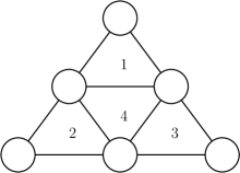
Figure 1: Sampling triangles does not lead to triangle sparsification.

Motif sparsification based on a triangle-weighted graph?

A natural way to apply Karger’s approach to our motif sparsification problem (or triangle sparsification in the following discussion) is to use it on the triangle weighted graph $G_{\Delta}=(V,E,w_{\Delta})$, where $w_{\Delta}(e)$ is the number of triangles containing edge $e$ that has been used in the context of graph clustering [BGL16, TPM17]. Indeed, triangle weighted graphs have the useful property that the size of the cut $(S,V\setminus S)$ in $G_{\Delta}$ is exactly twice the number of triangles that cross this cut in $G$. Therefore, if we were to sparsify $G$ to $G^{\prime}$ in such a way that $G^{\prime}_{\Delta}$ is a cut sparsifier of $G_{\Delta}$, $G^{\prime}$ would be a motif cut sparsifier of $G$. It is a seemingly natural approach to try to use triangle weighted graphs to obtain triangle sparsifiers. However, we will now show in a series of examples that a number of simple approaches which use the triangle weighted graph fail.

A naive approach using the triangle weighted graph would be to sparsify the triangle weighted graph, and then construct $G^{\prime}$ by taking the remaining edges in $G^{\prime}_{\Delta}$ with some weights. However, this does not work, as a situation could easily arise where all of the triangles in some cuts are deleted. Consider the example in Figure 2.

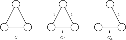
Figure 2: Sparsifying triangle weighted graph does not work for triangle sparsification.

Here, $G^{\prime}_{\Delta}$ is clearly a $1/2$-cut sparsifier of $G_{\Delta}$, but since it contains no triangles, no motif sparsifier of $G$ can be constructed from it without adding new edges.

A better approach is to apply Karger’s cut counting bound to the triangle weighted graph $G_{\Delta}$ and use it to prove that an appropriate random sample of edges of $G$, denoted by $G^{\prime}$, will satisfy

$$G_{\Delta}\approx_{\epsilon}G^{\prime}_{\Delta}.$$ (1)

First, in order to make this approach work, we need to assume that $G_{\Delta}$ is $k$-connected for some reasonably large $k$. We make this assumption now to illustrate the challenges that arise even in this special case. Following [Kar99], we could sample each edge with probability $\approx\frac{\log n}{k}$. That would unfortunately lead to each triangle staying in the graph with probability $\approx\frac{\log^{3}n}{k^{3}}$ only, and in particular some vertices may end up participating in no triangles in the sample with high probability. The latter means that the corresponding singleton cuts in $G^{\prime}_{\Delta}$ would be empty, and (1) would certainly not be satisfied. Naturally, we can also try to sample each edge with a lower probability, say $\approx\frac{\log n}{k^{2/3}}$, but in this case the number of edges in the sparsifier of a $k$-regular graph would be $\approx k^{1/3}n\log n$, which is in superlinear in $n$.

In general, the above attempts point to the fact that edge weights in $G^{\prime}_{\Delta}$ are a non-linear function of the random variables that govern the presence or absence of various edges in $G^{\prime}$, making ‘one-shot’ sparsification not easy to achieve.

Essential problem of triangle-weighted graph.

Although we have already outlined several problems that we encounter in our attempts to construct a sparsifier using the triangle-weighted graph, there is another fundamental problem which arises directly from its structure as the following example demonstrates.

Let the graph $G$ (see Figure 3) consist of a clique on vertices in $V(G)\setminus\{v_{1},\ldots v_{l}\}$ where $l=\lfloor\sqrt{n}\rfloor$, and let $h\leq\sqrt{n}/4$ be an integer. For $i\in[l]$, let vertex $v_{i}$ be connected with vertices $u_{i,1},\ldots,u_{i,l}$ such that the sets of neighboring vertices of $v_{1},\ldots,v_{l}$ don’t intersect. Notice that the subgraph induced by $V(G)\setminus\{v_{1},\ldots v_{l}\}$ has connectivity in $G_{\Delta}$ of at least $n(n-1)/8$, forming a connectivity component, while vertices $v_{1},\ldots,v_{l}$ are not a part of this component because they are only connected to the clique with at most $O(n)$ triangles each.

In this situation, the triangles $v_{i}u_{i,j_{1}}u_{i,j_{2}}$ for $i\in[l]$, $j_{1},j_{2}\in[h]$, and $j_{1}\neq j_{2}$ are “dangling”, i.e. one of their edges is part of a component with a high connectivity, while there is no such component containing the whole triangle.

We know from the first part of the introduction that there is a way to get a clique sparsifier with almost linear number of edges, and graph $G$ is a clique with additional $O(\sqrt{n})$ vertices and $O(n)$ edges. Since this is an insignificant part of the whole graph, one might think that it is still easy to get a sparsifier with almost linear number of edges, for example by taking all edges $v_{i}u_{i,j}$ with probability $1$, and sampling the clique as we did before. But we will now show that additional caution must be taken to handle the “dangling" triangles.

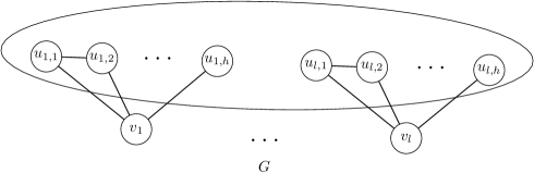
Figure 3: An illustration of “dangling” triangles.

First, suppose that we sample all of the edges in the clique with the probability $\leq 1/2$. Consider the case $h=2$. Then for all $i\in[l]$, edge $u_{i,1}u_{i,2}$ is contained in the only triangle in the cut $(\{v_{i}\},V(G)\setminus\{v_{i}\})$. With high probability, at least one of those cuts will have motif size $0$ and therefore, the resulting graph would not be motif sparsifier.

On the other hand, suppose that we were to take all of the edges $u_{i,j_{1}}u_{i,j_{2}}$ with probability $1$. Consider the case of $h=\lfloor\sqrt{n}/4\rfloor$. Then, the number of those edges would be $O(n^{3/2})$, and the sparsification would not produce any significant results. This shows that to take care of “dangling” triangles, we would need to sample the edges in them with different probabilities according to the situation at hand.

Under closer examination, one might discover that this problem stems from the following fact: consider a connectivity component $C$ in $G_{\Delta}$. If we were to take an induced subgraph of $G$ on vertices of $C$ and then build a triangle-weighted graph for it, the connectivity of this new triangle-weighted graph would most likely be lower than the connectivity of $C$.

As the above examples show, approaching motif sparsification purely from the point of view of sparsification of motif weighted graphs is difficult. Instead, we show, somewhat surprisingly, that a judicious composition of graph and hypergraph sparsification methods leads to a very clean approach, which we describe next. After that, we demonstrate that motif weighted graph can still be used in the proposed framework to achieve a speed-up in running time for dense graphs.

2.1 Strength-based sparsification

As we have discussed, it seems that we can neither use hypergraph nor graph sparsification ideas directly to obtain motif sparsifiers. The reason for this is probably that a motif is an object that — similarly to a hyperedge — usually lives on sets of more than 2 vertices, but at the same time is composed of edges, i.e. it is closely related to graphs. As a consequence motif sparsification may be viewed as an intermediate problem between hypergraph and graph sparsification.

Indeed, our main contribution is to properly combine ideas from graph and hypergraph sparsification and to overcome some motif specific technical obstacles. Our starting point will be to extend the notion of strong connectivity that is an important ingredient to many sparsification approaches (see, for example, [BK15, CX18]) to the realm of motifs. Here we follow the hypergraph view and conceptually treat motifs as hyperedges. This way we can immediately extend the notion of connected components in hypergraphs [CX18] to motifs by saying that a $k$-connected component is a maximal induced subgraph such that every cut is crossed by at least $k$ motif instances. This will allow us to define for each motif its importance as a measure of the amount it contributes to various cuts in the graph. The hypergraph view of motifs will also supply us with hypergraph cut counting arguments from [KK15a] that can be easily transferred to motif cuts and that will be useful for the analysis.

Once we have the definition of motif importance, it will be beneficial to switch to a graph-based view and think about how to compute the sparsifier. Our approach will be to sample edges but — similarly to earlier work in graph sparsification — we now need to identify important edges that we cannot miss for sparsification. In order to do so, we define the importance weight of an edge as the sum of the importance weights of its containing motifs. Edges whose importance weight is above a certain threshold will always be kept as sampling them would result in a variance that is too high.

For the remaining edges, we want to apply a sampling approach. Here, there are two more challenges. First, we need to deal with the non-linear behaviour of motif cut sizes and then we also need to address the fact that a motif is composed of several edges, which means that the events that two intersecting motifs are sampled is not independent, which means that we cannot use Chernoff bounds that are often used in the analysis of other sparsifying constructions. To deal with the non-linearity we observe that sparsifying by a constant factor is still possible and so we iteratively sparsify the graph $O(\log n)$ times by a constant. To deal with the dependencies in the sampling process and prove concentration, we use Azuma’s inequality. During the different stages, edges that are no longer contained in any motif will receive a weight of $0$ and will then be dropped.

Finally, we observe that except for the sets of critical edges, all edges are sampled with the same probability and so we can use our approach to compute a sparsifier that works simultaneously for a set of motifs.

2.2 Connectivity-based sparsification

A major drawback of the strength-based algorithm is the need to enumerate all instances of a given motif. This task is hard, since enumeration takes time that is at least proportional to the number of motive instances, which in dense graph ($|E|=O(n^{2})$) can easily reach $O(n^{r})$.

However, the motif cut sparsification task doesn’t implicitly require enumerating all of the motifs, and we show that by modifying an algorithm for exact subgraph counting [WW13], we can achieve sparsification in time $\widetilde{O}(n^{\omega\lceil r/3\rceil})$, which is sublinear to the number of motifs in dense graphs.

The key idea is to move away from using the importances based on motif strengths to importances based on motif connectivities, where the connectivity of a motif instance is the minimal motif size of a cut crossing this instance. This new measure of importance can be approximated without needing to enumerate all motifs, which leads to the faster (in some settings) running time of our second algorithm.

In more detail, we adopt the sparsification approach of [FHHP19] for our setting. A key object here is the motif weighted graph $G_{M}=(V,E,w_{M})$, where, similarly to the triangle weighted graph, each edge $e$ is reweighted to $w_{M}(e)$ – the sum of weights of motifs containing $e$. The main challenge is the approximation of motif-connectivity-based edge importance. This is done in two steps. First, we show that the connectivity of a motif instance is multiplicatively approximated by the minimum of motif connectivities of all edges in this instance, where the motif connectivity of an edge is the minimal size of a motif cut crossing this edge. Then, by dividing the graph into several layers, we are able to approximate the minimum-motif-connectivity-of-an-edge-based importance for each layer, which we then combine to get the final approximation.

The rest of the algorithm works in the same way as the first one, however we also use a result by [AKL⁺21] to compute all-pairs connectivities in $\widetilde{O}(n^{2})$ time. Our algorithm requires the motif connectivities of edges to be computed with multiplicative precision, which existing subquadratic approximation algorithms cannot deliver.

2.3 Overview of Lower Bound

In Section 8, we study the feasibility of producing a motif-cut sparsifier, similar to the one guaranteed by Theorem 1.2, in the setting where motif instances are required to be induced subgraphs. The main difficulty in attempting to sparsify induced motifs is that the act of removing edges from $G$ may result in new motif instances being created. This is not something we had to worry about in the proof of Theorem 1.2, and we could simply focus on preserving important motif instances that already existed in the original graph.

In fact, this difference turns out to result in a fundamental barrier, and we are able to show that any non-trivial sparsification may be impossible even for a motif as simple as the undirected $2$-path (see Theorem 1.3).

In our lower bound construction, the input graph will be the undirected, unweighted clique with the three edges of a specific triangle $(a,b,c)$ removed. More formally, we define $\Delta^{-}=(V,E_{\Delta}^{-})$ as an unweighted, undirected graph on $n$ vertices, where

$$E_{\Delta}^{-}=\binom{V}{2}\setminus\big{\{}\{a,b\},\{b,c\},\{c,a\}\big{\}},$$

for distinct special vertices $a,b,c\in V$.

Note that while our Graph $\Delta^{-}$ is dense, the number of induced motifs is small, and each motif is of constant size. In the case of non-induced motif-sparsification, this setting would be trivial, as we could simply keep all edges contributing to any motif, thereby sparsifying the graph, and retaining the exact cut structure. In the case of induced motifs, however, this doesn’t work, since removing edges may introduce additional motifs – as it would in this example.

Specifically, the number of induced motif instances of the $2$-path motif is exactly $3(n-3)$, with each motif instance containing $2$ of the special vertices. In Section 8.2, we essentially prove that any graph $\widehat{G}$ that would sparsify $\Delta^{-}$ should have (at least some of) these same $2$-paths present. As it does in $\Delta^{-}$, this would result in a very large (quadratic) number of not-necessarily-induced $2$-paths in $\widehat{G}$. In order to insure that these aren’t induced (and hence don’t count as motif instances) $\widehat{G}$ must be dense.

Example 1.

We give a slightly simpler – but ultimately incorrect – version of our above lower-bound construction for intuition. Consider the unweighted clique, with a single edge $(u,v)$ removed. More formally, $G=(V,E)$ is an unweighted undirected graph on $n$ vertices with

$$E=\binom{V}{2}\setminus\big{\{}\{u,v\}\big{\}}.$$

Attempting to sparsify this for the induced $2$-path motif, we can observe some of the same things as we do in our lower bound construction: Even though $G$ contains only a small, $\Theta(n)$, number of motifs, one cannot simply sparsify it by removing all edges that contribute to no motifs. The act of removing edges can create new induced $2$-paths, and we end up with a sparse graph whose induced-motif-cut structure doesn’t resemble that of $G$ at all.

In fact, one can prove (in a similar manner to the proof of Theorem 4.4) that no reweighted subgraph of $G$ approximates its induced-motif-cut structure, for some small constant $\epsilon$. Surprisingly however, there does exist a weighted graph which achieves an arbitrarily close estimation: Let $\widehat{G}=(V,\widehat{E},w)$ consist of the edge $\{u,v\}$ with weight $n^{2}$, and the $n-2$ edges in $u\times(V\setminus\{u,v\})$, each with weight $n^{-2}$. (This specificly gives a $(1\pm n^{-3})$-sparsifier, but the approximation can be arbitrarily improved by reweighting.) We leave the verification of the validity of this sparsifier to the reader.

3 Preliminaries

Let $G=(V,E,w)$ be a directed weighted graph with vertex set $V=\{1,\dots,n\}$ and edge set $E\subseteq V\times V$, $m:=|E|$. We will assume that the edge weights are always positive. Denote by $W=\max_{e\in E}w(e)/\min_{e\in E}w(e)$. In this paper, we study the connectivity structure of higher order patterns in the graph. More precisely, we consider a given directed graph $M=(V_{M},E_{M})$ which we assume to be a frequently occurring subgraph of $G$ and which we refer to as a network motif or motif for short [MSOI⁺02]. While the idea behind motifs is that they are more frequently occurring than what one would expect in a random graph [MSOI⁺02], we are not making any formal assumption of this kind during the paper. Still, our motivation is that the motifs are common subgraphs. We will always assume that motifs are weakly connected, i.e. the undirected version of the motif is connected. We make this assumption since we are interested in graph cuts; there is no convincing definition of a motif cut for motifs that have more than one weakly connected component. Formally, we define motifs as follows.

Definition 3.1 (Motifs and Motif Instances).

Let $M=(V_{M},E_{M})$ be a weakly connected directed graph which we refer to as a motif. A subgraph of $G$ that is isomorphic to $M$ is called an instance of motif $M$ in $G$. The set of all instances of a motif $M$ in $G$ is denoted $\mathcal{M}(G,M)$.

The definition of motifs extends to undirected graphs in a straightforward way by encoding undirected edges as two directed edges.

We will be interested in weighted graphs and therefore require a definition of weights of motif instances. In order to obtain such a definition, we first consider integer weighted graphs. A common interpretation of such graphs is that they can be viewed as unweighted multigraphs in which the multiplicity of each edge equals its weight. This view can be immediately generalized to define the weight of a motif of integer weighted graphs. We simply think of replacing every weighted edge by a corresponding number of copies and then count the number of distinct motifs. That is, the weight of a motif becomes the product of its edge weights. The extension to real non-negative weighted edges is straightforward.

Definition 3.2 (Weight of Motif Instance).

Let $G=(V,E,w)$ be a directed weighted graph. The weight $w(I)$ of a motif instance $I=(V_{I},E_{I})$ in $G$ is defined as

$$w(I)=\prod_{e\in E_{I}}w(e).$$

Let $(S,V\setminus S)$ be a cut in $G$. We say that motif instance $I=(V_{I},E_{I})$ crosses this cut if one of its edges crosses this undirected cut. Since the motifs are weakly connected by definition, this is equivalent to $V_{I}\cap S\neq\emptyset$ and $V_{I}\cap(S\setminus V)\neq\emptyset$.

Definition 3.3 (Motif Size of a Cut).

Let $G=(V,E,w)$ be a directed weighted graph. For a motif $M$ the $M$-motif size of cut $(S,V\setminus V)$ is defined as

$$\textup{Val}_{M,G}(S,V\setminus S)=\sum_{I\in\mathcal{M}(G,M):I\text{ crosses }(S,V\setminus S)}w(I).$$

Note that the previous definition is directly influenced by applied works such as [BGL16, YBLG17, TPM17] which also redefine the cut size in terms of the number of motifs crossing a cut.

Our goal is to construct an algorithm for sparsifying a graph in such a way that the motif sizes of all cuts are $(1\pm\epsilon)$ preserved. We formalize this notion as follows.

Definition 3.4.

Let $M=(V_{M},E_{M})$ be a motif and let $G=(V,E,w)$ be a directed weighted graph. A directed weighted graph $\widehat{G}$ is an $(M,\epsilon)$-motif cut sparsifier of $G$, if for every cut $(S,V\setminus S)$, the following holds:

$$(1-\epsilon)\textup{Val}_{M,G}(S,V\setminus S)\leq\textup{Val}_{M,\widehat{G}}(S,V\setminus S)\leq(1+\epsilon)\textup{Val}_{M,G}(S,V\setminus S).$$

3.1 Strong Motif Connectivity

We now extend the notion of strong connectivity used in graph cut sparsification [BK15] to motifs. For a given motif $M$ we will define the concepts of strong $M$-connectivity as well as $M$-connected components, which both follow naturally from the standard notion of strong connectivity. Our notion is also closely related to strong connectivity in hypergraphs [KK15a], if we view a motif as a hyperedge. The main difference is that motifs are composed of simpler objects, i.e. edges. Similarly to the case of graphs and hypergraphs, strong motif connectivity will allow us to get bounds on the number of distinct cuts that we need to consider in the analysis.

In graphs and hypergraphs one can now define sampling probabilities for edges or hyperedges and sample them accordingly. These probabilities are based on a definition of the strength of edges. It is tempting to follow the same approach for motif instances, however, as already discussed in the technical overview, there is a problem. If we sample a set of motif instances then their union may contain other motif instances that were not contained in the sample. The reason is simply that motifs are composed of edges. Therefore, later on, we will define an edge-based sampling procedure. It will still be useful for our purposes to define a notion of motif strength. We now give the formal definitions.

Definition 3.1.1 (Motif Connectivity).

Let $M=(V_{M},E_{M})$ be a motif, let $G=(V,E,w)$ be a directed weighted graph. $G$ is $(k,M)$-connected if every cut $(S,V\setminus S$) in $G$ has $M$-motif size at least $k$.

Definition 3.1.2 ($k$-Strong $M$-Connected Component).

Let $M=(V_{M},E_{M})$ be a motif, let $G=(V,E,w)$ be a directed weighted graph. For a value $k\in\mathbb{R}_{+}$, an induced subgraph $C=(V_{C},E_{C},w)$ of $G$ is called a $k$-strongly $M$-connected component of $G$, if

1. $C$ is $(k,M)$-connected and

2. there is no induced subgraph $C^{\prime}=(V_{C^{\prime}},E_{C^{\prime}},w)$ of $G$ that is $(k,M)$-connected and has $V_{C}\subsetneq V_{C^{\prime}}$.

We will consider two $M$-connected components distinct if their sets of vertices are distinct.

Definition 3.1.3 (Motif Strength).

Let $M=(V_{M},E_{M})$ be a motif, let $G=(V,E,w)$ be a directed weighted graph. Let $I\in\mathcal{M}(G,M)$ be a motif instance. The motif strength $\kappa_{I}$ of $I$ is the maximum value $k$ such that there exists a $(k,M)$-connected component that contains $I$ as a subgraph.

4 Main Results

In this section we present the main results of this paper. We express runtime and size bounds in $\widetilde{O}$ notation, which hides factors polynomial in $\log n$ and motif size. We start by stating the upper bound results in full generality:

Theorem 4.1.

Let $L>0$ be an integer. For every directed weighted graph $G=(V,E,w)$, $|V|=n$, every set of motifs $\{M_{i}\}_{i\in[L]}$ and every $\epsilon\in(0,1)$, a graph $G^{\prime}$ such that it is an $(M_{i},\epsilon)$-motif sparsifier of $G$ for all $i\in[L]$ with $\widetilde{O}(Ln/\epsilon^{2})$ edges can be computed in time

$$\widetilde{O}\left(L|E|+\sum_{i=1}^{L}T(G,M_{i})\right),$$

where $T(G,M_{i})$ for $i\in[L]$ is the time required to enumerate all instances of $M_{i}$ in $G$. The algorithm succeeds with probability at least $1-(L+1)n^{-c_{1}}$ for an arbitrarily large global constant $c_{1}$.

The main result of the paper is an immediate corollary:

Corollary 4.2.

For every graph $G=(V,E)$, $|V|=n$, every constant integer $k\geq 2$, $\epsilon\in(0,1)$, there exists an $\epsilon$-motif sparsifier $G^{\prime}$ of $G$ with respect to all motifs $M$ of size at most $k$ simultaneously that contains $\widetilde{O}(n/\epsilon^{2})$ edges. The graph $G^{\prime}$ can be constructed in polynomial time.

The second algorithm provides the following guarantee:

Theorem 4.3.

Let $L>0$ be an integer. For every directed weighted graph $G=(V,E,w)$, $|V|=n$, every set of motifs $\{M_{i}\}_{i\in[L]}$ and every $\epsilon\in(0,1)$, a graph $G^{\prime}$ such that it is an $(M_{i},\epsilon)$-motif sparsifier of $G$ for all $i\in[L]$ with $\widetilde{O}(Ln/\epsilon^{2})$ edges can be computed in time

$$\widetilde{O}(L(r^{r}+n^{\omega\lceil r/3\rceil})\log W),$$

where $r$ is the maximum number of vertices in $M_{i}$, $i\in[L]$, $W=\max_{e\in E}w(e)/\min_{e\in E}w(e)$ and $\omega<2.37286$ is the matrix multiplication constant [AW21]. The algorithm succeeds with probability at least $1-(L+1)n^{-c_{1}}$ for an arbitrarily large global constant $c_{1}$.

Although the two algorithms are very similar, there are cases when the first algorithm is faster than the second one. It would still be so even if we were to construct the motif weighted graph through enumeration. This is because computing all-pairs connectivities takes $\widetilde{O}(n^{2})$ time, while the first algorithm can work in nearly-linear time with respect to the number of motifs. This is relevant when, for example, we have only one motif — triangle — and $|E|=O(n^{4/3-\delta})$ for $\delta>0$. Then enumeration can be done in time $O(|E|^{3/2})=O(n^{2-3\delta/2})$ producing at most $O(|E|^{3/2})$ motif instances.

Last but not least, we derive a negative result on the possibility of constructing a motif cut sparsifier for induced motif instances. The definitions of motif cut size and motif cut sparsifier are straightforwardly adapted from non-induced case by counting only induced motif instances as motif instances. See Section 8 for details.

Theorem 4.4.

Let $f(n)=o(n^{2})$ and let $\varepsilon,0<\varepsilon\leq 1/500$. There exists a motif $M=(V_{M},E_{M})$ such that for every sufficiently large integer $n$, there exists a graph $G=(V,E)$ on $n$ vertices, such that it is impossible to construct an $(M,\epsilon)$-induced-motif cut sparsifier for $G$ with $f(n)$ non-negatively weighted edges.

Notice that this also includes graphs that are not subgraphs of the original graph.

The paper is organised as follows. In Section 5 we introduce Algorithm 1 (PartialSparsification) for sparsifying an input graph by a constant factor while preserving its motif cut structure; we analyze this algorithm in Sections 5 and 5.1. Then, in Section 6 we introduce Algorithm 2 (MotifSparsification ), and prove that it achieves the guarantees of Theorem 4.1, which we prove at the end of the section. Finally, in Section 8, we present and prove our main lower bound result.

5 Overview and analysis of PartialSparsification

In this section we will develop the main algorithmic tool of this paper — a procedure we call PartialSparsification (Algorithm 1) that with high probability sparsifies any graph (with sufficiently many edges) by a constant factor while approximately maintaining the motif cut sizes for a set of motifs. Once we have this procedure available, we can iterate it $\Theta(\log n)$ times to obtain our final sparsifier. Details can be found in Section 6.

Let $\{M_{1},\ldots,M_{L}\}$ be a set of motifs. We aim to obtain a graph $G^{\prime}$ such that it is a $(\epsilon,M_{i})$-motif cut sparsifier of $G$ simultanuously for all $M_{i}$, $i\in[L]$. For $i\in[L]$, denote $r_{i}=|V_{M_{i}}|$ and $r^{*}_{i}=|E_{M_{i}}|$ as the size of the vertex and edge set of the $i$-th motif respectively; denote $r_{max}=\max_{i\in[L]}r_{i}$, $r^{*}_{max}=\max_{i\in[L]}r^{*}_{i}$ as the largest $r_{i}$ and $r^{*}_{i}$ value among all $i\in[L]$, respectively. As we will see, the running time and the sparsifier size depends on $r_{max}$ and $r^{*}_{max}$.

In our proofs, we will use a sufficiently small constant $d>0$, as well a constant $c_{1}>0$ which will govern the success probability of the algorithm. The value of $d$ depends on $c_{1}$; this dependency is determined in Lemma 5.2.5. The value of $c_{1}$ is arbitrary; we can for example assume that $c_{1}=10$ (this would ultimately lead to the failure probability being at most $n^{-4}$).

Our procedure PartialSparsification is very simple. It identifies a set of critical edges that have to be included in the sparsifier as sampling them would result in too high variance. The remaining edges will be taken with constant probability $p$. One may simply set $p=1/2$. However, our analysis implies that the size of the set of critical edges increases exponentially in $1/p$ and it turns our that a better choice will be $p=2^{-1/{(2r^{*}_{max})}}$ as this balances the number of repetitions needed to sparsify the graph and the size of the set of critical edges.

We start by introducing definitions used in the algorithm.

Definition 5.1 (Motif Weight of an Edge).

Let $\mathcal{M}=(V_{M},E_{M})$ be a motif and $G=(V,E,w)$ be a directed weighted graph. Then the $M$-motif weight of an edge $w_{M}(e)$ is defined as

$$w_{M}(e)=\sum_{I\in\mathcal{M}(G,M):e\in E(I)}w(I).$$

Definition 5.2 (Importance Weight).

Let $M=(V_{M},E_{M})$ be a motif and $G=(V,E,w)$ be a directed weighted graph. Then

• for $I\in\mathcal{M}(G,M)$ the importance weight in $G$ is $\eta(I)=w(I)/\kappa_{I}$,

• for an edge $e\in E$, the $M$-importance weight in $G$ is

  $$\eta_{M}(e)=\sum_{I\in\mathcal{M}(G,M):e\in E(I)}\eta(I).$$

We now formally define our notion of critical edges.

Definition 5.3 (Critical Edge).

Let $M=(V_{M},E_{M})$ be a motif and $G=(V,E,w)$ be a directed weighted graph. An edge $e$ is called $M$-critical if the $M$-importance weight of $e$ is at least $\frac{d\epsilon^{\prime 2}}{r^{*}(\log n+r)}$.

While it is possible to compute the strengths of all motif instances exactly, it can be computationally expensive. Instead, we will approximate them.

Lemma 5.4 (Follows from Theorem 6.1 of [CX18], Strength Estimation).

There exists algorithm StrengthEstimation which does the following: it receives as an input a directed weighted graph $G=(V,E,w)$ and a motif instance set $\mathcal{M}(G,M)$ for a motif $M=(V_{M},E_{M})$ and outputs strength estimations $\kappa^{\prime}_{I}$ for each motif instance $I\in\mathcal{M}(G,M)$ with the following properties:

1. For all $I\in\mathcal{M}(G,M)$, $\kappa^{\prime}_{I}\leq\kappa_{I}$,

2. $\sum_{I\in\mathcal{M}(G,M)}\frac{w(I)}{\kappa^{\prime}_{I}}\leq cr(n-1)$, for some constant $c>0$

where $r=|V_{M}|$. The running time of the algorithm is $O(r|\mathcal{M}(G,M)|\log^{2}n\log(r|\mathcal{M}(G,M)|))$.

We defer the discussion of this algorithm and proof of this lemma to Section 5.4.

Since we don’t have access to the motif instance strengths in our algorithm, we need to define a version of importance weight that uses strength approximations.

Definition 5.5.

Let $M=(V_{M},E_{M})$ be a motif and $G=(V,E,w)$ be a directed weighted graph. Let $\kappa^{\prime}_{I}$ be the estimations produced by the algorithm from Lemma 5.4 for the graph $G$ for the motif $M$.

• For $I\in\mathcal{M}(G,M)$ the estimated importance weight is $\widehat{\eta}(I)=w(I)/\kappa^{\prime}_{I}$,

• For an edge $e\in E$, the estimated $M$-importance weight is

  $$\widehat{\eta}_{M}(e)=\sum_{I\in\mathcal{M}(G,M):e\in E(I)}\widehat{\eta}(I).$$

We can now present the Algorithm 1.

Algorithm 1 Partial Sparsification

1:procedure PartialSparsification($V,E,w,\epsilon^{\prime},\{\mathcal{M}(G,M_{i})\}_{i=1}^{L}$)

2:     Calculate $\mathcal{M}(G,M_{i})$ for all $i\in[L]$ for graph $G=(V,E,w)$

3:     $E_{+}\leftarrow\emptyset$

4:     for $i=1\to L$ do

5:         $\{\kappa^{\prime}_{I}\}_{I\in\mathcal{M}(G,M_{i})}\leftarrow\textsc{StrengthEstimation}(G,\mathcal{M}(G,M_{i}))$

6:         $E_{+}\leftarrow E_{+}\cup\{e\in E:\widehat{\eta}_{M_{i}}(e)\geq\frac{d\epsilon^{\prime 2}}{r^{*}_{i}(\log n+r_{i})}\}$ $\triangleright$ Find critical edges

7:     end for

8:     $E_{-}\leftarrow\emptyset$

9:     $w^{\prime}\leftarrow w$

10:     for $e\in E\setminus E_{+}$ do

11:         if a probability $p=2^{-1/{(2r^{*}_{max})}}$ Bernoulli variable is equal to $1$ then

12:              $w^{\prime}(e)\leftarrow w(e)/p$

13:         else

14:              $w^{\prime}(e)\leftarrow 0$

15:              $E_{-}\leftarrow E_{-}\cup\{e\}$

16:         end if

17:     end for

18:     $E\leftarrow E\setminus E_{-}$

19:     return $(E,w^{\prime})$

20:end procedure

5.1 Analysis of $E_{+}$

In this and following subsections, we will show that PartialSparsification indeed produces an $(\epsilon^{\prime},M)$-motif cut sparsifier of the input graph $G=(V,E)$.

Fix one of the motifs among $M_{1},\ldots,M_{L}$ as $M$, and denote $r=|V(M)|$, $r^{*}=|E(M)|$. From here on we will show a number of properties of our algorithm that would eventually allow us to show that the final graph is a $M$-motif cut sparsifier. Since it will generally not involve any other motifs, we will omit mentioning $M$ in subscripts and other places where appropriate until Section 6.1.

$E_{+}$ is a set produced by PartialSparsification. Recall that we want to sample each critical edge with probability $1$ and each other edge with probability $p$. In fact, what happens in the algorithm is that all of the edges in $E_{+}$ are sampled with probability $1$ and all other edges are sampled with probability $p$. Therefore, to show the correctness of the algorithm, it is necessary to show that $E_{+}$ contains all of the critical edges. Moreover, since on each iteration the graph loses about $1-p$ fraction of the edges not in $E_{+}$, it is necessary for us to bound the number of edges in $E_{+}$ in order to bound the number of edges in the output graph. We do both in this section.

Denote

$$E_{M+}=\left\{e\in E_{1}:\widehat{\eta}_{M}(e)\geq\frac{d\epsilon^{\prime 2}}{r^{*}(\log n+r)}\right\}.$$

First, we show that $E_{M+}$ (and consequently $E_{+}$) contains all $M$-critical edges:

Lemma 5.1.1.

The set $E_{+}$ in line 6 of Algorithm 1 contains all $M$-critical edges.

Proof.

By Lemma 5.4,

$$\forall I\in\mathcal{M}(G,M):\kappa^{\prime}_{I}\leq\kappa_{I}.$$

By definition of $M$-critical edge and importance weight,

$$\sum_{I\in\mathcal{M}(G,M):e\in E(I)}\frac{w(I)}{\kappa_{I}}\geq\frac{d\epsilon^{\prime 2}}{r^{*}\log n}.$$

On the other hand,

$$\sum_{I\in\mathcal{M}(G,M):e\in E(I)}\frac{w_{M}(I)}{\kappa_{I}}\leq\sum_{I\in\mathcal{M}(G,M):e\in E(I)}\frac{w_{M}(I)}{\kappa^{\prime}_{I}}=\widehat{\eta}_{M}(e).$$

Therefore, the condition in line 6 of Algorithm 1 holds for $e$, which means that $E_{+}$ contains all $M$-critical edges. ∎

Furthermore, we have that $E_{+}=\bigcup_{i=1}^{L}E_{M_{i}+}$, hence by bounding $E_{M+}$ we can bound $E_{+}$.

Lemma 5.1.2.

The size of $E_{M+}$ is at most $\frac{cr(r^{*})^{2}(n-1)(\log n+r)}{d\epsilon^{\prime 2}}$.

Proof.

By Lemma 5.4, the following holds:

$$\sum_{I\in\mathcal{M}(G,M)}\widehat{\eta}(I)\leq cr(n-1).$$

We can bound the sum of estimations of importance weight of all edges:

$$\sum_{e\in E}\widehat{\eta}_{M}(e)=\sum_{e\in E}\sum_{\begin{subarray}{c}I\in\mathcal{M}(G,M):\\ e\in E(I)\end{subarray}}\widehat{\eta}(I)\leq r^{*}\sum_{I\in\mathcal{M}(G,M)}\widehat{\eta}(I)\leq crr^{*}(n-1).$$

On the other hand, since edges in $E_{+M}$ must satisfy inequality in line 6 of Algorithm 1, we have

$$|E_{M+}|\cdot\frac{d\epsilon^{\prime 2}}{r^{*}(\log n+r)}\leq\sum_{e\in E_{M+}}\widehat{\eta}_{M}(e)\leq\sum_{e\in E}\widehat{\eta}_{M}(e).$$

Combining both inequalities yields:

$$|E_{M+}|\leq\frac{cr(r^{*})^{2}(n-1)(\log n+r)}{d\epsilon^{\prime 2}},$$

as desired. ∎

Corollary 5.1.3.

$E_{+}$ satisfies

$$|E_{+}|\leq\frac{cLr_{max}{(r^{*}_{max})^{2}}(n-1)(\log n+r_{max})}{d\epsilon^{\prime 2}}.$$

Proof.

The proof follows from Lemma 5.1.2 by summing across all motifs. ∎

5.2 Correctness of PartialSparsification

As in [BK15], to show the correctness of our algorithm, we want to split our graph $G$ into a “sum” of several weighted graphs. The decomposition may be viewed as the motif-version of the decomposition of Benczur and Karger [BK15] and follows rather closely their ideas.

Let $k_{1},\ldots,k_{h}$ be all of the different strong $M$-connectivity values in $G$ in increasing order, i.e. for each $k_{i}$ there exists a $k_{i}$-connected component that is not $k$-connected for any $k>k_{i}$. Let $k_{0}=0$. In order to decompose our graph into a sum of weighted graphs we observe that we can write

$$\textup{Val}_{M,G}(S,V\setminus S) = \sum_{\begin{subarray}{c}I\in\mathcal{M}(G,M):\\ I\text{ crosses }(S,V\setminus S)\end{subarray}}w(I)$$

$$= \sum_{\begin{subarray}{c}I\in\mathcal{M}(G,M):\\ I\text{ crosses }(S,V\setminus S)\end{subarray}}\frac{w(I)}{\kappa_{I}}\cdot\kappa_{I}$$

$$= \sum_{\begin{subarray}{c}I\in\mathcal{M}(G,M):\\ I\text{ crosses }(S,V\setminus S)\end{subarray}}\frac{w(I)}{\kappa_{I}}\cdot\left(\sum_{i:k_{i}\leq\kappa_{I}}k_{i}-k_{i-1}\right)$$

$$= \sum_{i=1}^{h}(k_{i}-k_{i-1})\cdot\sum_{\begin{subarray}{c}I\in\mathcal{M}(G,M):\\ \kappa_{I}\geq k_{i}\end{subarray}}\frac{w(I)}{\kappa_{I}}\cdot{\mathbbm{1}}(I\text{ crosses }(S,V\setminus S))$$

where the third equality follows from $\kappa_{I}=\sum_{i:\kappa_{I}\geq k_{i}}k_{i}-k_{i-1}$ and where ${\mathbbm{1}}(I\text{ crosses }(S,V\setminus S))$ denotes the indicator function that motif instance $I$ crosses the cut $(S,V\setminus S)$. The above formula guides us towards our decomposition. The sum

$$\sum_{\begin{subarray}{c}I\in\mathcal{M}(G,M):\\ \kappa_{I}\geq k_{i}\end{subarray}}\frac{w(I)}{\kappa_{I}}\cdot{\mathbbm{1}}(I\text{ crosses }(S,V\setminus S))$$

ranges over all motif instances that are contained in components of $M$-connectivity at least $k_{i}$. We will now view the graph as a sum of graphs $F_{i}$ where each $F_{i}$ is the union of all $(k_{i},M)$-connected components of $G$. The motif instances in the graph $F_{i}$ will be weighted by a factor of $k_{i}-k_{i-1}$. In addition, each motif $I$ is reweighted by $1/\kappa_{I}$ in all graphs $F_{i}$. This motivates the following definition.

Definition 5.2.1.

Let $M=(V_{M},E_{M})$ be a motif and $G=(V,E,w^{\prime})$ be a directed weighted graph. For a weighted graph $H=(V_{H},E_{H},w)$ with $V_{H}\subseteq V$ and $E_{H}\subseteq E$ and a cut $(S,V_{H}\setminus S)$ , we define the following value:

$$\widetilde{\textup{Val}}_{M,H}(S,V_{H}\setminus S)=\sum_{\begin{subarray}{c}I\in\mathcal{M}(H,M):\\ I\text{ crosses }(S,V_{H}\setminus S)\end{subarray}}\frac{w(I)}{\kappa_{I}(G)},$$

where $\kappa_{I}(G)$ is the motif strength of $I$ with respect to $G$.

In the following we will always use the above definition in a way that $G$ is the input graph of PartialSparsification. We will also frequently use $G$ as a subscript when the subgraph $H$ in the above definition equals $G$. Using the above notation we can now write

$$\textup{Val}_{M,G}(S,V\setminus S) = \sum_{i=1}^{h}(k_{i}-k_{i-1})\cdot\widetilde{\textup{Val}}_{M,F_{i}}(S,V\setminus S)$$ (2)

$$= \sum_{i=1}^{h}(k_{i}-k_{i-1})\cdot\sum_{\begin{subarray}{c}\text{ $k_{i}$-connected}\\ \text{component }C\end{subarray}}\widetilde{\textup{Val}}_{M,C}(S,V\setminus S)$$ (3)

where the last equality splits $F_{i}$ into its $M$-connected components.

Now, our goal is to show the concentration result for a single $M$-connected component. There are two well-known results for hypergraph cuts that can be adapted for the case of motifs that we need to use to show concentration for all cuts. We include their proofs for completeness.

Lemma 5.2.2 (Reformulation of Theorem 6.8 of [CX18]).

Let $M=(V_{M},E_{M})$ be a motif and $G=(V,E,w)$ be a directed weighted graph. If minimum of $\widetilde{\textup{Val}}_{M,G}$ of all non-trivial cuts is greater than $0$, it is equal to $1$.

Proof.

Let $(S,V\setminus S)$ be the cut with minimum motif size and let $k$ be the $M$-connectivity of $G$. Then all of the motif instances crossing the cut have connectivity exactly $k$. On the other hand, the size of cut is $k$, which gives us

$$\widetilde{\textup{Val}}_{M,G}(S,V\setminus S)=\sum_{I\in\mathcal{M}(G,M):I\text{ crosses }(S,V\setminus S)}\frac{w(I)}{\kappa_{I}}=\frac{\textup{Val}_{M,G}(S,V\setminus S)}{k}=1.$$

Consider any other cut $(S,V\setminus S)$ of motif size $k^{\prime}$. Then the strength of all motif instances crossing this cut is at most $k^{\prime}$, which means that:

$$\widetilde{\textup{Val}}_{M,G}(S,V\setminus S)=\sum_{I\in\mathcal{M}(G,M):I\text{ crosses }(S,V\setminus S)}\frac{w(I)}{\kappa_{I}}\geq\frac{\textup{Val}_{M,G}(S,V\setminus S)}{k^{\prime}}=1.$$

Therefore, the cut with the minimum motif size is the cut with the minimum value of $\widetilde{\textup{Val}}_{M,G}$, and the latter is equal to $1$. ∎

Lemma 5.2.3 (Motif Cut Counting, Reformulation of Theorem 3.2 of [KK15a]).

Let $M=(V_{M},E_{M})$ be a motif and $G=(V,E,w)$ be a directed weighted graph. Let $c$ be the minimum value of $\widetilde{\textup{Val}}_{M,G}$ across all cuts in $G$. There are at most $O(2^{(\alpha+1)r}n^{2(\alpha+1)})$ cuts with value $\widetilde{\textup{Val}}_{M,G}$ at most $\alpha c$ for a real $\alpha\geq 1$.

The proof of the above lemma is given in Section 5.4.

In the works on graph and hypergraph sparsification the value of a cut is defined by the edges or hyperedges. These are also the objects that are sampled and it suffices to use a Chernoff bound to analyze the concentration of a fixed cut. In our case, we sample edges but we are interested in the number of motif instances that cross the cut. We can write the cut value as a sum of random variables corresponding to the motifs that cross the cut, but these random variables are not independent and so we cannot use Chernoff bounds. To deal with dependencies we will instead use Azuma’s inequality.

Lemma 5.2.4 (Azuma’s Inequality, [Azu67]).

Let $Z_{0},Z_{1},\ldots,Z_{n}$ be a martingale satisfying $|Z_{i}-Z_{i-1}|\leq c_{i}$ for each $i\in[n]$. For any $\lambda>0$,

$$\mathbb{P}(|Z_{n}-Z_{0}|\geq\lambda)\leq 2\exp\left(\frac{-\lambda^{2}}{2(c_{1}^{2}+\cdots+c_{n}^{2})}\right).$$

We will use this lemma with a special ‘edge-exposure’ martingale, which will be defined in the proof of Lemma 5.2.5.

Lemma 5.2.5.

Let $C$ be a $M$-connected component before the application of PartialSparsification and $C^{\prime}$ be that subgraph after the application. The following holds with probability at least $1-n^{-c_{1}}$:

Let $V_{C}=V(C)$. For all cuts $(S,V_{C}\setminus S)$ of $C$,

$$(1-\epsilon^{\prime})\widetilde{\textup{Val}}_{M,C}(S,V_{C}\setminus S)\leq\widetilde{\textup{Val}}_{M,C^{\prime}}(S,V_{C}\setminus S)\leq(1+\epsilon^{\prime})\widetilde{\textup{Val}}_{M,C}(S,V_{C}\setminus S).$$

Proof.

By applying Lemma 5.2.2 to $C$, we get that the minimum of values $\widetilde{\textup{Val}}_{M,C}$ across all cuts in $C$ is $1$.

Note that all of the critical edges in $C$ are critical in $G$, since their $M$-importance weight in $C$ is not larger than in $G$. Since, by Lemma 5.1.1, $E_{+}$ contains all critical edges in $G$, it also contains all of the critical edges in $C$, and, therefore, no critical edges are being sampled afterwards. Fix a cut $(S,V_{C}\setminus S)$ with $\widetilde{\textup{Val}}_{M,C}(S,V_{C}\setminus S)=\alpha\geq 1$ in $C$. Let $E_{2}$, $t:=|E_{2}|$, be the set of all edges that are being sampled in PartialSparsification with probability $p=2^{-1/{(2r^{*}_{max})}}\geq 2^{-1/{(2r^{*})}}$ and that are part of at least one motif cut by $(S,V_{C}\setminus S)$. Then $E_{2}$ does not contain any critical edges. Let $I_{0}$ be the subgraph of $C$ containing all vertices and edges that are a part of some motif that is being cut by $(S,V_{C}\setminus S)$.

Consider the following random process: enumerate the edges in $E_{2}$ in the order they are being examined by PartialSparsification. Suppose edge $e$ with number $i$ is being sampled. If $e$ is not sampled, then we define $I_{i}$ to be equal to $I_{i-1}$ without $e$, otherwise $I_{i}$ is equal to $I_{i-1}$ with $e$ with it’s weight multiplied by $1/p$. Now consider a random process $X_{i}$, $i\in\{0,\ldots,t\}$, where $X_{i}$ is equal to $\widetilde{\textup{Val}}_{M,I_{i}}(S,V_{C}\setminus S)$.

It is easy to see that $X_{t}=\widetilde{\textup{Val}}_{M,C^{\prime}}(S,V_{C}\setminus S)$ and that $X_{i}$ is a martingale. Let

$$M^{S}(e)=\sum_{\begin{subarray}{c}I\in\mathcal{M}(C,M):\\ e\in E(I),\\ I\text{ crosses }(S,V_{C}\setminus S)\end{subarray}}\frac{w_{M}(I)}{\kappa_{I}}.$$

Then $|X_{i}-X_{i-1}|\leq M^{S}(e)/p^{r^{*}}$, where $e$ is the edge being sampled on step $i$, since the weight of all motifs can change by at most $1/p^{r^{*}}$ during the random process. Note that although the weight of $e$ changes at most by a factor of $1/p$ the weights of other edges of any motif may have increased by a factor of $1/p$ earlier in the process. Since $M^{S}(e)$ is defined at the beginning of the process, we can only bound the increase by a factor of $1/p^{r^{*}}$. Therefore, to apply Lemma 5.2.4, we need to bound $\sum_{e\in E_{2}}M^{S}(e)^{2}$.

Since there are no critical edges in $E_{2}$, for all edges $e$ that we sample, we must have

$$M^{S}(e)\leq\frac{d\epsilon^{\prime 2}}{r^{*}(\log n+r)}.$$

On the other hand,

$$\sum_{e\in E_{2}}M^{S}(e)\leq r^{*}\sum_{I\in\mathcal{M}(C,M):I\text{ crosses }(S,V_{C}\setminus S)}\frac{w_{M}(I)}{\kappa_{I}}=r^{*}\alpha,$$

since every motif contains at most $r^{*}$ edges. Therefore, using this inequality:

$$\sum_{e\in E_{2}}M^{S}(e)^{2}\leq\frac{d\epsilon^{\prime 2}}{r^{*}(\log n+r)}\sum_{e\in E_{2}}M^{S}(e)\leq\frac{\alpha d\epsilon^{\prime 2}}{\log n+r}.$$

Hence, because $\widetilde{\textup{Val}}_{M,C}(S,V_{C}\setminus S)=\alpha$ and by Lemma 5.2.4,

$$\mathbb{P}(|\widetilde{\textup{Val}}_{M,C}(S,V_{C}\setminus S)-\widetilde{\textup{Val}}_{M,C^{\prime}}(S,V_{C}\setminus S)|\geq\epsilon^{\prime}\widetilde{\textup{Val}}_{M,C}(S,V_{C}\setminus S))\leq\mathbb{P}(|X_{t}-X_{0}|\geq\epsilon^{\prime}\alpha)$$

$$\leq 2\exp\left(\frac{-(\epsilon^{\prime}\alpha)^{2}}{2\sum_{e\in E_{2}}M^{S}(e)/p^{2r^{*}}}\right)\leq 2\exp\left(\frac{-(\epsilon^{\prime}\alpha)^{2}}{4\cdot\frac{\alpha d\epsilon^{\prime 2}}{\log n+r}}\right)=2\exp\left(\frac{-\alpha(\log n+r)}{4d}\right).$$

We now apply a union bound on all cuts $(S,V_{C}\setminus S)$ in conjunction with Lemma 5.2.3. We need to bound $\sum_{\alpha\geq 1}P(\alpha)g(\alpha)$, where $P(\alpha)$ is the probability that the inequalities in the statement of the lemma doesn’t hold for the cut with $\widetilde{\textup{Val}}_{M,C}$ equal to $\alpha$, $g(\alpha)$ is the number of those cuts, and the sum is taken across all values of $\alpha$ that are present in the graph.

Let $F(\alpha)=\sum_{\alpha\geq\alpha^{\prime}\geq 1}g(\alpha^{\prime})$ be the total number of cuts with $\widetilde{\textup{Val}}_{M,C}\leq\alpha$. By Lemma 5.2.3, $F(\alpha)=A2^{(\alpha+1)r}n^{2(\alpha+1)}$ for some constant $A$. We then adversarialy extend $F(\alpha)$ in a to the whole $\mathbb{R}_{+}$ such that $F(\alpha)$ is differentiable while preserving the above inequality.

We have that

$$\sum_{\alpha\geq 1}P(\alpha)g(\alpha)\leq\int_{1}^{\infty}P(\alpha)\frac{dF(\alpha)}{d\alpha}d\alpha.$$

Therefore, by applying partial integration,

$$\int_{1}^{\infty}P(\alpha)\frac{dF(\alpha)}{d\alpha}d\alpha=\Big{[}P(\alpha)F(\alpha)\Big{]}_{1}^{\infty}-\int_{1}^{\infty}F(\alpha)\frac{dP(\alpha)}{d\alpha}d\alpha$$

$$\leq 2A2^{2r}n^{4}\exp\left(-\frac{\log n+r}{4d}\right)+\int_{1}^{\infty}An^{2(x+1)}2^{r(x+1)}\frac{\log n+r}{4d}2\exp\left(-\frac{x(\log n+r)}{4d}\right)dx$$

$$\leq n^{-c_{1}}$$

by setting $d$ to be sufficiently small. Thus, the inequalities in the lemma statement hold with probability at least $1-n^{-c_{1}}$ for all cuts, as desired. ∎

We will now use the fact that for a given cut, we can take the weighted sum of the $\widetilde{\textup{Val}}_{M,C}$ of cuts of each of the connectivity components $C$ such that this sum is equal to the motif cut size in the whole graph. We can then apply Lemma 5.2.5 to each term to obtain the cut preservation property for the whole graph.

Lemma 5.2.6.

Let $G^{\prime}$ be $G$ after the application of PartialSparsification. $G^{\prime}$ is $(M,\epsilon^{\prime})$-motif cut sparsifier of $G$ with probability $1-n^{-c_{1}+3}$.

Proof.

By definition of motif cut sparsifier, it is enough to show that the following holds for all cuts $(S,V\setminus S)$ of $G$:

$$(1-\epsilon^{\prime})\textup{Val}_{M,G}(S,V\setminus S)\leq\textup{Val}_{M,G^{\prime}}(S,V\setminus S)\leq(1+\epsilon^{\prime})\textup{Val}_{M,G}(S,V\setminus S).$$

By equation (3), we have

$$\textup{Val}_{M,G}(S,V\setminus S) = \sum_{i}(k_{i}-k_{i-1})\cdot\sum_{\begin{subarray}{c}\text{ $k_{i}$-connected}\\ \text{component }C\end{subarray}}\widetilde{\textup{Val}}_{M,C}(S,V\setminus S).$$

Now let $C^{\prime}$ be $C$ after the application of PartialSparsification. Then, similarly, the following holds:

$$\textup{Val}_{M,G^{\prime}}(S,V\setminus S) = \sum_{i}(k_{i}-k_{i-1})\cdot\sum_{\begin{subarray}{c}\text{ $k_{i}$-connected}\\ \text{component }C\text{ in }G\end{subarray}}\widetilde{\textup{Val}}_{M,C^{\prime}}(S,V\setminus S).$$

Note that if two $M$-connected components intersect, one of them is contained inside the other, and the smaller one has higher connectivity. Therefore, the set of all $M$-connected components is a laminar family, which means that its size is at most $2n$. By applying Lemma 5.2.5 to all $(k_{i},M)$-connected components $C$ for all $i$ and a union bound over the at most $2n$ different $M$-connected components, the following holds for all $M$-connected components:

$$(1-\epsilon^{\prime})\widetilde{\textup{Val}}_{M,C^{\prime}}(S,S\setminus V)\leq\widetilde{\textup{Val}}_{M,C}(S,S\setminus V)\leq(1+\epsilon^{\prime})\widetilde{\textup{Val}}_{M,C^{\prime}}(S,S\setminus V)$$

with probability at least $1-2n^{-c_{1}+1}\geq 1-n^{-c_{1}+3}$. Combining all of the equalities and inequalities, we get the claim. ∎

5.3 Hypergraphs

We introduce hypergraphs here since we will use some results concerning them. A hypergraph is the pair of two sets $(V,F)$, where $V$ is the set of vertices and $F$ is the set of hyperedges $f$, which are subsets of $V$. Weighted hypergraph $H=(V,F,w)$ is a hypergraph with weight function $w:F\to\mathbb{R}_{+}$. A hypergraph $H$ is $r$-uniform if every $f\in F$ satisfies $|f|=r$. We denote the size of the cut $(S,V\setminus S)$ in hypergraph $H$ as $\textup{Val}_{H}(S,V\setminus S)$.

Definition 5.3.1 (Induced Subhypergraph).

A hypergraph $H^{\prime}=(V^{\prime},F^{\prime},w^{\prime})$ is an induced subhypergraph of a hypergraph $H=(V,F,w)$, if $V^{\prime}\subseteq V$, $F^{\prime}=\{f\in F:f\subseteq V^{\prime}\}$ and $w$ and $w^{\prime}$ are equal on $F^{\prime}$.

We will abuse the cut notation for the hypergraphs: if $H^{\prime}=(V^{\prime},F^{\prime},w)$ is an induced subhypergraph of $H=(V,F,w)$, then $\textup{Val}_{H^{\prime}}(S,V\setminus S):=\textup{Val}_{H^{\prime}}(S\cap V^{\prime},V^{\prime}\setminus S)$.

Definition 5.3.2 (Connectivity).

A weighted hypergraph $H=(V,F,w)$ is $k$-connected if every cut $(S,V\setminus S$), $S\neq\emptyset$, $S\subsetneq V$, in $H$ has size at least $k$.

Definition 5.3.3 ($k$-connected Component).

For a weighted hypergraph $H=(V,F,w)$ with non-negative hyperedge weights and a value $k\in\mathbb{R}_{+}$, an induced subhypergraph $C=(V_{C},F_{C},w)$ of $H$ is called a $k$-connected component of $H$, if

1. $C$ is $k$-connected and,

2. there is no induced subhypergraph $C^{\prime}=(V_{C^{\prime}},F_{C^{\prime}},w)$ of $G$ that is $k$-connected and has $V_{C}\subsetneq V_{C^{\prime}}$.

Definition 5.3.4 (Hyperedge Strength).

Let $H=(V,F,w)$ be a weighted hypergraph with non-negative hyperedge weights. A hyperedge $f\in F$ has strength $\kappa_{f}$ if $\kappa_{f}$ is the maximum value of $k$ such that there exists a $k$-connected component of $H$ that contains $f$.

5.4 Strength Estimation and Motif Cut Counting

To reiterate, construction of motif cut sparsifier is not possible by only using the techniques for constructing hypergraph sparsifier. But, the problems are sufficiently close to share some similarities, which allows us to use some results for hypergraph cut sparsification in our proof.

In this section we will present omitted proofs of Lemma 5.4 and Lemma 5.2.3 by reducing them to similar existing results for hypergraphs.

Because motif instances are essentially just subsets of vertices, it is useful to consider them as hyperedges of some hypergraph, which we will call a motif hypergraph. Note that some motif instances share the same set of vertices. In this case, the weight of the resulting hyperedge is equal to the sum of their weights.

Definition 5.4.1 (Motif Hypergraph).

Let $M=(V_{M},E_{M})$ be a motif and $G=(V,E,w)$ be a directed weighted graph. Then the $M$-motif hypergraph of $G$ is an undirected weighted hypergraph $H_{M}=(V,F_{M},w_{M})$, where

• $F_{M}=\{V(I):I\in\mathcal{M}(G,M)\}$,

• for $f\in F_{M}$, $w_{M}(f)=\sum_{I\in\mathcal{M}(G,M):f=V(I)}w(I)$.

Note that the motif hypergraph represents the motif connectivity structure of a graph: for a cut $(S,V\setminus S)$ in $G$, its motif size is equal to it’s size in $H$, and for a $I\in\mathcal{M}(G,M)$, $\kappa_{I}=\kappa_{V(I)}$ where $V(I)$ is a hyperedge of motif hypergraph. The introduction of hypergraph allows us to use several results from hypergraph cut sparsification, as well as giving a new perspective on the problem.

We now prove Lemma 5.4 by using the following result.

Lemma 5.4.2 (Theorem 6.1 of [CX18], Strength Estimation).

There exists algorithm StrengthEstimation which does the following: it receives as an input a rank $r$ weighted hypergraph $H=(V,F,w)$ on $n$ vertices and outputs strength estimations $\kappa^{\prime}_{f}$ for each hyperedge $f$ with the following properties:

1. For all $f\in F$, $\kappa^{\prime}_{f}\leq\kappa_{f}$,

2. $\sum_{f\in F}\frac{w(s)}{\kappa^{\prime}_{f}}\leq cr(n-1)$, for some constant $c>0$.

The running time of the algorithm is $O(r|F|\log^{2}n\log(r|F|))$.

Note that although the algorithm presented in [CX18] can only work with natural weights, we can easily reduce the general case to it by dividing all of the weights by the minimum one and then rounding them down to the nearest integer: tt only worsens the second property by a factor of $2$.

Proof of Lemma 5.4.

We construct motif hypergraph $H_{M}$ and run the algorithm from Lemma 5.4.2 on it, then set $\kappa^{\prime}_{I}:=\kappa^{\prime}_{V(I)}$ for $I\in\mathcal{M}(G,M)$. Since the construction of $H_{M}$ takes only $O(|\mathcal{M}(G,M)|)$ time, the total runtime is the same as in Lemma 5.4.2, and both properties straightforwardly follow from properties of $H_{M}$. ∎

Finally, we give the proof of Lemma 5.2.3.

Lemma 5.4.3 (Cut Counting in Hypergraphs, Theorem 3.2 of [KK15a]).

In an $r$-uniform weighted hypergraph $H=(V,M,w)$ with size of minimum cut $c$, there are at most $O(2^{\alpha r}n^{2\alpha})$ cuts of size no more than $\alpha c$ for a half-integer $\alpha\geq 1$ where $\alpha$ is a half-integer if $2\alpha$ is an integer.

Proof of Lemma 5.2.3.

Consider a modification of a motif hypergraph, where each hyperedge’s weight is divided by its strength. Denote it by $H^{\prime}$. It is easy to see that the size of an arbitrary cut $(S,V\setminus S)$ in $H^{\prime}$ is equal to the $\widetilde{\textup{Val}}_{M,G}(S,V\setminus S)$. Indeed,

$$\textup{Val}_{H^{\prime}}(S,V\setminus S) =\sum_{f\in F:f\text{ crosses }(S,V\setminus S)}\frac{w_{M}(f)}{\kappa_{f}}$$

$$=\sum_{I\in\mathcal{M}(G,M):I\text{ crosses }(S,V\setminus S)}\frac{w(I)}{\kappa_{I}}$$

$$=\widetilde{\textup{Val}}_{M,G}(S,V\setminus S).$$

Therefore, it is enough to show that if $c$ is the size of the smallest cut in $H^{\prime}$, the number of cuts of size $\alpha c$ is at most $O(2^{(\alpha+1)r}n^{2(\alpha+1)})$, which we achieve as follows: find the smallest half integer $\beta\geq\alpha$ and apply Lemma 5.4.3 to it and $H^{\prime}$. The result then follows from the fact that $\beta<1+\alpha$. ∎

5.5 Runtime of PartialSparsification

Theorem 5.5.1.

Let a directed weighted graph $G=(V,E,w)$, $\epsilon^{\prime}\in(0,1)$ and a set of motifs $\{M_{i}\}_{i\in[L]}$ be the input of PartialSparsification. The total running time of PartialSparsificationis

$$\sum_{i=1}^{L}T(G,M_{i})+\widetilde{O}\left(L|E|+\sum_{i=1}^{L}|\mathcal{M}(G,M_{i})|\right),$$

where $T(G,M_{i})$ for $i\in[L]$ is the time required to enumerate all instances of $M_{i}$ in $G$.

Proof.

We will analyze each of the procedures. StrengthEstimation takes time $O(r_{i}|\mathcal{M}(G,M_{i})|\cdot\log^{2}n\cdot\log(r_{i}|\mathcal{M}(G,M_{i})|))$ by Lemma 5.4 for each $M_{i}$. Computing the values $\widehat{\eta}_{M_{i}}(e)$ and finding all critical edges can be done in $O(r^{*}_{i}|\mathcal{M}(G,M_{i})|+|E|)$ time for $i\in[L]$. We repeat those steps for all $L$ motifs. Sampling edges in the loop requires $O(|E|)$ operations. On top of that, the algorithm calculates $\mathcal{M}(G,M_{i})$ and $H_{M_{i}}$, which requires $\sum_{i=1}^{L}T(G,M_{i})+O(\sum_{i=1}^{L}{r^{*}_{i}}|\mathcal{M}(G,M_{i})|)$ time, resulting in the total running time of

$$\sum_{i=1}^{L}T(G,M_{i})+O\left(\sum_{i=1}^{L}(r_{i}|\mathcal{M}(G,M_{i})|\cdot\log^{2}n\cdot\log(r_{i}|\mathcal{M}(G,M_{i})|)+r^{*}_{i}|\mathcal{M}(G,M_{i})|+|E|)\right).\qed$$

6 Analysis of MotifSparsification

We are now ready to analyze the complete algorithm, MotifSparsification. As was mentioned before, it essentially only calls PartialSparsification  $O(r^{*}_{max}\log n)$ times. Hence, our main goal in this section is to show that after all these applications, the graph is still $(\epsilon,M_{i})$-motif sparsifier for all $i\in[L]$.

Because we also have the Algorithm 4 utilizing the same sparsification approach, we will show a proof for a generic algorithm, GeneralPartialSparsification, which abstracts both of the partial sparsification algorithms.

Definition 6.1.

We assume that GeneralPartialSparsification accepts as input a weighted directed graph $G=(V,E,w)$, $\varepsilon^{\prime}>0$, and a set of motifs $\{M_{i}\}_{i=1}^{L}$, and returns $(E^{\prime},w^{\prime})$ such that $G^{\prime}=(V,E^{\prime},w^{\prime})$ is $(\varepsilon^{\prime},M_{i})$-motif cut sparsifier for all $i\in[L]$ with probability at least $1-n^{-c_{1}}$ obtained through sampling at most $A$ of the edges with probability $1$ and the rest of the edges with probability $2^{-1/(2r^{*}_{max})}$ in time $B$. $A$ and $B$ can depend both on input parameters, as well as on the constant $c_{1}$.

Algorithm 2 Motif Sparsification

1:procedure MotifSparsification($G,\{M_{i}\}_{i\in[L]},\epsilon$) $\triangleright$ $G=(V,E,w)$

2:     $\epsilon^{\prime}\leftarrow\frac{\epsilon}{5c_{1}r^{*}_{max}\log n}$ $\triangleright$ $c_{1}$ is an absolute constant, $r^{*}_{max}$ is maximum motif size

3:     $E_{0}\leftarrow\emptyset$

4:     for $j=1$ to $\lceil 2c_{1}r^{*}_{max}\log n\rceil$ do

5:         $(E,w)\leftarrow\textsc{GeneralPartialSparsification}{}(V,E,w,\epsilon^{\prime},\{M_{i}\}_{i=1}^{L})$

6:     end for

7:     return $G=(V,E,w)$

8:end procedure

Since the approximation error grows multiplicatively after each application of GeneralPartialSparsification, we will need Lemma A.1 to get a final approximation bound.

Lemma 6.2.

At the end of the MotifSparsification, the set $E$ contains at most $A$ edges with probability at least $1-n^{-c_{1}+2}$.

Proof.

Since all edges, except for those that are sampled with probability $1$, are sampled independently with same probability (and we only care about their quantity) and since the number of edges sampled with probability $1$ is bounded by $A$, we can assume without loss of generality that those are the same edges each time.

Consider an arbitrary edge $e\in E$ at the start of the loop. Assume that $e$ is present in $E$ at the end of the algorithm. If it was sampled each time with probability $2^{-1/{(2r^{*}_{max})}}$, the probability of this happening is at most

$$(2^{-1/{(2r^{*}_{max})}})^{2c_{1}r^{*}_{max}\log n}=n^{-c_{1}}.$$

Since there are at most $n(n-1)$ edges in $G$, the probability that at least one of those edges will be present in $E$ is less than $n^{-c_{1}+2}$ by a union bound. Therefore, $E$ consists entirely of edges sampled with probability $1$ with probability at least $1-n^{-c_{1}+2}$, hence it’s size is at most $A$. ∎

Lemma 6.3.

Let a directed weighted graph $G=(V,E,w)$, $\epsilon\in(0,1)$ and a set of motifs $\{M_{i}\}_{i\in[L]}$ be the input of MotifSparsification and $G^{\prime}$ be its output. Then for an arbitrary $M\in\{M_{i}\}_{i\in[L]}$, $G^{\prime}$ is $(M,\epsilon)$-motif cut sparsifier of $G$ with probability at least $1-n^{-c_{1}+5}$ for a sufficiently large $n$.

Proof.

By definition, $G^{\prime}$ is a $(M,\epsilon)$-motif cut sparsifier if for all cuts $(S,V\setminus S)$, we have

$$(1-\epsilon)\textup{Val}_{M,G}(S,V\setminus S)\leq\textup{Val}_{M,G^{\prime}}(S,V\setminus S)\leq(1+\epsilon)\textup{Val}_{M,G}(S,V\setminus S).$$

We now proceed to show that the above inequalities hold. Denote by $l=\lceil 2c_{1}r^{*}_{max}\log n\rceil$ the number of loop iterations and denote by $G_{j}=(V,E_{j},w_{j})$ the state of the graph at the end of the loop iteration $j$ where $G_{0}=G$. We will prove the following inductive statement:

With probability at least $1-jn^{-c_{1}+3}$, the following holds after loop iteration $j$: For any cut $(S,V\setminus S)$ of $G$, the following holds:

$$(1-\epsilon^{\prime})^{j}\textup{Val}_{M,G}(S,V\setminus S)\leq\textup{Val}_{M,G_{j}}(S,V\setminus S)\leq(1+\epsilon^{\prime})^{j}\textup{Val}_{M,G}(S,V\setminus S).$$

Note that for $j\leq l$, $(1+\epsilon^{\prime})^{j}\leq(1+\frac{\epsilon}{2l})^{l}\leq 1+\epsilon\leq 2$ and, similarly $(1-\epsilon^{\prime})^{j}\geq 1-\epsilon/2\geq 1/2$ by Lemma A.1 and since $\epsilon\leq 1$.

Base case: for $j=0$, the property is trivial.

Inductive step: suppose that the statements hold for $j-1$. We can apply Lemma 5.2.6, which, combined with inductive assumption, gives us the property.

The probability that the used lemma fails is at most $n^{-c_{1}+3}$. Therefore, by a union bound with the probability that inductive assumption holds, the probability that the statement for iteration $j$ holds is at least $1-jn^{-c_{1}+3}$.

Since $G^{\prime}=G_{l}$, the inductive assumption on the last iteration also holds for $G^{\prime}$, which means that:

$$(1-\epsilon)\textup{Val}_{M,G}(S,V\setminus S)\leq(1-\epsilon^{\prime})^{l}\textup{Val}_{M,G}(S,V\setminus S)\leq\textup{Val}_{M,G^{\prime}}(S,V\setminus S),$$

which gives us the desired lower bound. The upper bound is proven similarly. In total, the failure probability is at most $l\cdot n^{-c_{1}+3}$, which is less then $n^{-c_{1}+5}$ for a sufficiently large $n$. ∎

6.1 Multiple Motifs

We now put together all of our preceding lemmas to get our final sparsification result for all motifs simultaneously.

Lemma 6.1.1.

Let a directed weighted graph $G=(V,E,w)$, $\epsilon\in(0,1)$ and a set of motifs $\{M_{i}\}_{i\in[L]}$ be the input of MotifSparsification and $G^{\prime}$ be it’s output. Then with probability at least $1-L\cdot n^{-c_{1}+5}$, $G^{\prime}$ is $M_{i}$-motif cut $(1+\epsilon)$ sparsifier of $G$ for all $i\in[L]$ for a sufficiently large $n$.

Proof.

The proof follows from applying Lemma 6.3 to each of the motifs $M_{i}$, $i\in[L]$. ∎

Lemma 6.1.2.

Let a directed weighted graph $G=(V,E,w)$, $\epsilon\in(0,1)$ and a set of motifs $\{M_{i}\}_{i\in[L]}$ be the input of MotifSparsification. The total running time of MotifSparsification is $O(r^{*}_{max}B\log n)$.

Proof.

Immediate from the fact that $B$ is the runtime of GeneralPartialSparsification. ∎

6.2 MotifSparsification with PartialSparsification

Proof of Theorem 4.1.

The proof follows from Lemma 6.1.1, Lemma 6.2 and Lemma 6.1.2.

By Corollary 5.1.3, the number of edges in the final graph is at most

$$\frac{cLr_{max}{(r^{*}_{max})^{2}}(n-1)(\log n+r_{max})}{d\epsilon^{\prime 2}} =O\left(\frac{Lr_{max}{(r^{*}_{max})^{4}}(n-1)(\log n+r_{max})\log^{2}n}{\epsilon^{2}}\right)$$

$$=\widetilde{O}(Ln/\epsilon^{2}).$$

To improve upon runtime a little bit, in PartialSparsification, we can compute each set of motif instances only once, since we only delete them during the algorithm. Since the algorithm calls PartialSparsification in a loop the total runtime is

$$\sum_{i=1}^{L}T(G,M_{i})+$$

$$O\left(\sum_{i=1}^{L}{(r^{*}_{max})}^{2}|\mathcal{M}(G,M_{i})|\cdot\log n+r_{max}^{*}r_{i}|\mathcal{M}(G,M_{i})|\cdot\log^{3}n\cdot\log(r_{i}|\mathcal{M}(G,M_{i})|)+|E|)\right)$$

$$=\sum_{i=1}^{L}T(G,M_{i})+\widetilde{O}\left(L|E|+\sum_{i=1}^{L}|\mathcal{M}(G,M_{i})|\right).\qed$$

7 Sparsification without enumeration

One of the main problems of the presented algorithm is that it requires finding every motif instance, which takes time at least equal to the number of motif instances, which can reach $O(n^{r})$ in dense graphs.

Nevertheless, there is still a way to circumvent the enumeration. Consider the case when the sparsification is performed with respect to only one motif $M$. Recall that PartialSparsification on a high level does two things: finds critical edges and samples non-critical edges with high probability. The importance of the edge is defined as the sum of importances of motifs containing this edge:

$$\eta_{M}(e)=\sum_{I\in\mathcal{M}(G,M):e\in E(I)}\eta(I),$$

where $\eta(I)=w(I)/\kappa_{I}$, and the edge is critical if $\eta_{M}(e)\geq\frac{d\epsilon^{\prime 2}}{r^{*}(\log n+r)}$.

It is easy to see that all steps of this procedure can be performed in time $\widetilde{O}(|E|+|V|)$, except for computing the values $\eta_{M}(e)$. This is why we opt for a different approach of defining importances, based on connectivities.

7.1 Basic Definitions

Definition 7.1.1 (Motif Connectivity).

Let $M=(V_{M},E_{M})$ be a motif, let $G=(V,E,w)$ be a directed weighted graph. Let $I\in\mathcal{M}(G,M)$ be a motif instance. The connectivity, $k_{I}$ of $I$ is the minimum $M$-motif size of a cut $(S,V\setminus S)$ which $I$ crosses.

Accordingly, we adopt the following notation.

Definition 7.1.2 (Connectivity Importance Weight).

Let $M=(V_{M},E_{M})$ be a motif and $G=(V,E,w)$ be a directed weighted graph. Then

• for $I\in\mathcal{M}(G,M)$, the connectivity importance weight in $G$ is $\mu(I)=w(I)/k_{I}$,

• for an edge $e\in E$, the connectivity $M$-importance weight in $G$ is

  $$\mu_{M}(e)=\sum_{I\in\mathcal{M}(G,M):e\in E(I)}\mu(I).$$

While it is unclear how to compute motif strengths without enumerating all motifs, there is a way to approximate motif connectivities. The key idea is to compute the motif weighted graph, and then use the edge connectivities there to bound the motif connectivities, since the cut sizes in motif weighted graph are close to the $M$-motif sizes of corresponding cuts in the original graph.

Definition 7.1.3 (Motif Weighted Graph).

Let $M=(V_{M},E_{M})$ be a motif and $G=(V,E,w)$ be a directed weighted graph. The undirected graph $G_{M}=(V,E,w_{M})$ is called the $M$-motif weighted graph. (Recall from Definition 5.1 that $w_{M}(e)=\sum_{I\in\mathcal{M}(G,M):e\in E(I)}w(I)$.) The motif weighted graph should be considered as undirected.

Although it was shown by [FHHP19] that graph cut sparsification is possible using the importances based on connectivities, to our knowledge no previous work has shown that it is possible in the hypergraph setting. Hence to show the correctness of the proposed algorithm, we shall adapt their techniques to our approach.

Finally, to compute the motif weighted graph we shall modify an algorithm for computing the number of motif instances in the graph [WW13].

The following sections will be organized as follows: we will first present the algorithm for computing the motif weighted graph and prove its correctness and runtime, followed by the sparsification algorithm. In the rest of this section we will introduce necessary definitions and show some of their properties.

Definition 7.1.4 ($M$-connectivity of an edge).

Let $M=(V_{M},E_{M})$ be a motif and $G=(V,E,w)$ be a directed weighted graph. Recall that the connectivity of an edge $e$ in graph $G_{M}$ is the minimum size of a cut cutting $e$ in $G_{M}$. For $e\in E$, the value $k_{M,e}$, equal to the connectivity of an edge $e$ in the motif weighted graph $G_{M}$, is called $M$-connectivity of the edge $e$.

We will be omitting subscript $M$ where possible.

Definition 7.1.5.

Let $M=(V_{M},E_{M})$ be a motif and $G=(V,E,w)$ be a directed weighted graph. Then

• for $I\in\mathcal{M}(G,M)$, the estimated connectivity importance weight in $G$ is

  $$\nu(I)=w(I)\frac{r^{*}}{\min_{e\in E(I)}k_{M,e}},$$

• for an edge $e\in E$, the estimated connectivity $M$-importance weight in $G$ is

  $$\nu_{M}(e)=\sum_{I\in\mathcal{M}(G,M):e\in E(I)}\nu(I).$$

Lemma 7.1.6.

Let $M=(V_{M},E_{M})$ be a motif and $G=(V,E,w)$ be a directed weighted graph. For any cut $(S,V\setminus S)$, the following holds:

$$\textup{Val}_{M,G}(S,V\setminus S)\leq\textup{Val}_{G_{M}}(S,V\setminus S)\leq r^{*}\textup{Val}_{M,G}(S,V\setminus S).$$

In addition, for all $I\in\mathcal{M}(G,M)$,

$$\mu(I)\leq\nu(I)\leq r^{*}\cdot\mu(I).$$

Proof.

The first property follows from the following observation: if a cut cuts a motif, then it cuts between $1$ and $r^{*}$ of its edges. Therefore, the contribution of a motif $I$ to the size of a cut that crosses it in $G_{M}$ is between $w(I)$ and $r^{*}w(I)$.

To establish the second property, notice that for all $I\in\mathcal{M}(G,M)$, by definition of edge connectivity,

$$\min_{e\in E(I)}k_{M,e}=\min_{e\in E(I)}\min_{\emptyset\subsetneq S\subsetneq V:(S,V\setminus S)\text{ cuts }e}\textup{Val}_{G_{M}}(S,V\setminus S)=\min_{\emptyset\subsetneq S\subsetneq V:(S,V\setminus S)\text{ cuts }I}\textup{Val}_{G_{M}}(S,V\setminus S).$$

This, in combination with the first property, leads to

$$k_{I}\leq\min_{e\in E(I)}k_{M,e}\leq r^{*}k_{I},$$

which implies the second property. ∎

7.2 Constructing the motif weighted graph

Most of the algorithmic ideas in this section are adopted from [WW13]. The design of the algorithm is based on the idea of reducing the task of computing the number of motif instances in graph $G$ to the task of computing the number of triangles in a specially constructed graph $G_{\sigma}$, with a one-to-one correspondence between motif instances in $G$ and triangle instances in $G_{\sigma}$. Then, we can apply fast matrix multiplication to count the number of triangles in $G_{\sigma}$.

The problem of computing a motif weighted graph is slightly different from the problem of computing the number of motifs. We can use the latter in a black box manner: for each edge $e\in E$, we delete this edge from the graph and compute the number of remaining motif instances. The difference between this number and the number of motif instances in the original graph is the motif weight of the edge $e$. This approach requires calling the motif counting primitive $|E|+1$ times. In this subsection, we present an algorithm which can construct the motif graph without this additional factor of $|E|$ in the running time.

7.2.1 Notation

Most of the notation in this subsection is exclusive to this subsection. We fix the motif $M=(V_{M},E_{M})$, and we will be omitting it where possible. Denote by $T_{k}=\{(v_{1},\ldots,v_{k}):\forall j\in[k]\>v_{j}\in V\land\forall j,i\in[k]\>j\neq i\rightarrow v_{i}\neq v_{j}\}$ the set of all ordered sequences of $k$ distinct vertices of $G$.

Let $k_{1},k_{2},k_{3}$ be such that $k_{1}+k_{2}+k_{3}=r$, and $\lfloor r/3\rfloor\leq k_{i}\leq\lceil r/3\rceil$. The algorithm starts by constructing a tripartite graph with weighted vertices and edges $G_{\sigma}=(V_{\sigma},E_{\sigma},w_{\sigma})$ defined as follows: $V_{\sigma}=T_{k_{1}}\cup T_{k_{2}}\cup T_{k_{3}}$, where we consider the entries of the three parts $T_{k_{i}}$ to be distinct. Fix some arbitrary ordering $\pi$ of vertices $V_{M}$, and let $\pi_{1}$ be its first $k_{1}$ entries, $\pi_{2}$ the next $k_{2}$ entries, and $\pi_{3}$ the rest of its entries.

For a vertex $v\in T_{k_{i}}\subset V_{\sigma}$, consider a natural mapping $f_{v}:v\to V_{M}$, where for $\ell\in[k_{i}]$, $f_{v}(v_{l})=\pi_{i,\ell}$. Note that if we are also given $u\in T_{k_{j}}$ and $z\in T_{k_{h}}$, where $i,j,h$ are $1,2,3$ in some order, and $v,u,z$ are pairwise disjoint, we can construct natural extensions of the corresponding mappings: $f_{v,u}=f_{v}\cup f_{u}$ and $f_{v,u,z}=f_{v}\cup f_{u}\cup f_{z}$. Notice that both of them, as well as $f_{v}$, are bijections. We call such a mapping $f$ consistent if $f^{-1}$ is a graph homomorphism (that is every edge in $M$, when mapped via $f^{-1}$, corresponds to an edge in $G$). We denote by $E(f)$ the subset of edges $E$ that are mapped to edges in $E_{M}$.

For a vertex $v\in T_{k_{i}}\subset V_{\sigma}$, its weight is defined to be equal to

$$w_{\sigma}(v)=\prod_{e\in E(f_{v})}w(e),$$

if $f_{v}$ is consistent, and $0$ if it is not. For a pair of vertices $u,v\in V_{\sigma}$, there is an edge between them if they come from different sets $T_{k_{i}}$, are pairwise disjoint, and mapping $f_{u,v}$ is consistent. The weight of the edge $(u,v)$ is equal to

$$w_{\sigma}((u,v))=\prod_{e\in E(u,v)}w(e),$$

where $E(u,v)=\{e\in E(f_{u,v}):|e\cap u|=|e\cap v|=1\}$.

Lemma 7.2.1.

$P$ is an injective graph homomorphism between $G_{M}$ and a subgraph $G^{\prime}$ of $G$ iff there exists a triangle $u,v,z\in V_{\sigma}$ such that $P=f^{-1}_{u,v,z}$.

Proof.

The reverse direction is easy to see. Since there is only an edge between two vertices if they are pairwise disjoint, come from different sets $T_{k_{i}}$, and $f_{u,v},f_{v,z}$, and $f_{v,z}$ are consistent, it follows that $f_{u,v,z}$ is consistent and, therefore, $P$ is a homomorphism.

In the other direction, suppose that $P$ maps $\pi_{1}$ to $u$, $\pi_{2}$ to $v$, $\pi_{3}$ to $z$. Since $P$ is injective, $u$, $v$ and $z$ are pairwise disjoint and don’t contain repeating elements. Therefore, they are vertices of $G_{\sigma}$, and, since $P$ is homomorphism, by definition they are pairwise connected by edges. By definition of $f_{u,v,z}$, $f^{-1}_{u,v,z}=P$. ∎

The approach now is to compute the triangle weighted graph for $G_{\sigma}$, and use it to construct the motif weighted graph of the original graph. The triangle weighted graph we construct differs somewhat from the motif weighted graph defined in Definition 7.1.3, since we must take into account the vertex-weights in $G_{\sigma}$. Formally, denote by $\Delta$ the triangle motif, i.e. the clique on $3$ vertices. For $I\in\mathcal{M}(G_{\sigma},\Delta)$, define

$$w_{\sigma}(I)=\prod_{v\in V(I)}w_{\sigma}(v)\prod_{e^{\prime}\in E(I)}w_{\sigma}(e^{\prime}).$$

For $e\in E_{\sigma}$, define

$$w_{\Delta,\sigma}(e)=\sum_{I\in\mathcal{M}(G_{\sigma},\Delta):e\in E(I)}w_{\sigma}(I)$$

and for $v\in V_{\sigma}$,

$$w_{\Delta,\sigma}(v)=\sum_{I\in\mathcal{M}(G_{\sigma},\Delta):v\in V(I)}w_{\sigma}(I).$$

Let $A$ denote the number of automorphisms of $M$.

Lemma 7.2.2.

For $e\in E$,

$$w_{M}(e)=\frac{1}{A}\left(\sum_{v\in V_{\sigma}:e\in E(f_{v})}w_{\Delta,\sigma}(v)+\sum_{(u,v)\in E_{\sigma}:e\in E(u,v)}w_{\Delta,\sigma}((u,v))\right)$$

Proof.

Let $w^{\prime}_{M}(e)$ be the weighted sum of all vertex-ordered instances of $M$ containing $e$. Then, trivially, $w^{\prime}_{M}(e)=A\cdot w_{M}(e)$. Each vertex-ordered instance of $M$ is uniquely defined by an injective homomorphism $P$ from $G_{M}$ to a subgraph of $G$, with its weight being:

$$w(P)=\prod_{e\in P(E_{M})}w(e),$$

where $P(E_{M})=\{(P(u),P(v)):(u,v)\in E_{M}\}$ is the projection of the edges of $M$.

By Lemma 7.2.1, $P$ uniquely maps to a triple of vertices $u,v,z$ forming a triangle. Since the set of edges $P(E_{M})=E(f_{u,v,z})$ can be partitioned into sets of edges between elements of $u$, $v$ and $z$, and between pairs of elements from different vertices,

$$w(P)=\prod_{e\in P(E_{M})}w(e)=\prod_{v\in V(I)}w_{\sigma}(v)\prod_{e^{\prime}\in E(I)}w_{\sigma}(e^{\prime})=w_{\sigma}(I),$$

where $I=(u,v,z)$ is the aforementioned triangle. Therefore

$$w^{\prime}_{M}(e)=\sum_{I\in\mathcal{M}(G_{\sigma},\Delta):e\in E(I)}w_{\sigma}(I).$$

Note that for a triangle $I=(u,v,z)$, edge $e\in E$ can only be present in one of the sets

$$E(f_{v}),E(f_{u}),E(f_{z}),E(u,v),E(u,z),E(v,z),$$

since $u,v,z$ are pairwise disjoint, and that those sets form a partition of $E(I)$. Therefore

$$w^{\prime}_{M}(e)=\sum_{I\in\mathcal{M}(G_{\sigma},\Delta)}w_{\sigma}(I)=\sum_{v\in V_{\sigma}:e\in E(f_{v})}w_{\Delta,\sigma}(v)+\sum_{(u,v)\in E_{\sigma}:e\in E(u,v)}w_{\Delta,\sigma}((u,v)).$$

The claim now follows from the relation $w^{\prime}_{M}(e)=A\cdot w_{M}(e)$. ∎

7.2.2 Analysis of the algorithm

We can now present the Algorithm 3. Let $N(v)$ be the set of vertices adjacent to $v\in V_{\sigma}$.

Algorithm 3 Constructing the motif weighted graph

1:procedure MotifWeights($G=(V,E,w),M=(V_{M},E_{M})$)

2:     Compute number of automorphisms $A$ of $M$.

3:     Construct graph $G_{\sigma}=(V_{\sigma},E_{\sigma})$.

4:     Let $W$ be the weighted adjacency matrix of $G_{\sigma}$.

5:     Let $D$ be a diagonal matrix with diagonal entries $w_{\sigma}(v),v\in V_{\sigma}$.

6:     $U\leftarrow DWDWD$

7:     for $(u,v)\in E_{\sigma}$ do

8:         $w_{\Delta,\sigma}((u,v))\leftarrow W_{u,v}\cdot U_{u,v}$.

9:     end for

10:     for $v\in V_{\sigma}$ do

11:         $w_{\Delta,\sigma}(v)\leftarrow\frac{1}{2}\sum_{u\in N(v)}w_{\Delta,\sigma}((u,v))$

12:     end for

13:     $\forall e\in E:w^{\prime}_{M}(e)\leftarrow 0$

14:     for $v\in V_{\sigma}$, $e\in E(f_{v})$ do

15:         $w^{\prime}_{M}(e)\leftarrow w^{\prime}_{M}(e)+w_{\Delta,\sigma}(v)$

16:     end for

17:     for $(u,v)\in E_{\sigma}$, $e\in E(u,v)$ do

18:         $w^{\prime}_{M}(e)\leftarrow w^{\prime}_{M}(e)+w_{\Delta,\sigma}((u,v))$

19:     end for

20:     return $w^{\prime}_{M}/A$

21:end procedure

Theorem 7.2.3.

Let a directed weighted graph $G=(V,E,w)$ and a motif $M=(V_{M},E_{M})$ be the input of MotifWeights. Then Algorithm 3 returns the function $w_{M}(e),e\in E$.

Proof.

Assuming that values $w_{\Delta,\sigma}$ are computing correctly by the algorithm, Lemma 7.2.2 implies that the values $w^{\prime}_{M}$ and $w_{M}$ are also computed correctly. Therefore, we only need to prove correctness of computation of $w_{\Delta,\sigma}$.

To show that, notice that $w_{\sigma}((u,v))=W(u,v)=0$ if $u$ and $v$ are not connected. Therefore, for $(u,v)\in E_{\sigma}$:

$$w_{\Delta,\sigma}((u,v))= \sum_{I\in\mathcal{M}(G_{\sigma},\Delta):e\in E(I)}w_{\sigma}(I)$$

$$=\sum_{z\in V_{\sigma}:(u,z)\in E_{\sigma}\land(z,v)\in E_{\sigma}}w_{\sigma}(u)w_{\sigma}((u,z))w_{\sigma}(z)w_{\sigma}((z,v))w_{\sigma}(v)w_{\sigma}((u,v))$$

$$=\sum_{z\in V_{\sigma}}D_{u,u}W_{u,z}D_{z,z}W_{z,v}D_{v,v}W_{u,v}=(DWDWD)_{u,v}W_{u,v},$$

which is exactly what is being computed. Considering values $w_{\Delta,\sigma}$ for vertices, the following equality holds

$$w_{\Delta,\sigma}(v)=\frac{1}{2}\sum_{u\in N(v)}w_{\Delta,\sigma}((u,v))$$

since each triangle containing $v$ will be counted twice in the sum on the right hand side. ∎

Theorem 7.2.4.

Let a directed weighted graph $G=(V,E,w)$ and a motif $M=(V_{M},E_{M})$ be the input of MotifWeights. Then its running time is $O(n^{\omega\lceil r/3\rceil}+r^{2}n^{2\lceil r/3\rceil}+r^{*}r^{r})$ where $n^{\omega}$ is matrix multiplication time.

Proof.

The number of automorphisms can be computed in time $O((r^{*}+r)r^{r})$, by checking all $r!$ permutations of vertices of $M$.

The graph $G_{\sigma}$ has $O(n^{\lceil r/3\rceil})$ vertices and $O(n^{2\lceil r/3\rceil})$ edges, and can be constructed in time $O((r+r^{*})n^{2\lceil r/3\rceil})$. Using fast matrix multiplication ([AW21] is state-of-the art at the time of writing), $U$ can be computed in time $O(n^{\omega\lceil r/3\rceil})$.

The rest of the algorithm can be computed in time $O(r^{2}(|V_{\sigma}|+|E_{\sigma}|))=O(r^{2}n^{2\lceil r/3\rceil})$, which gives the final runtime

$$O(n^{\omega\lceil r/3\rceil}+r^{2}n^{2\lceil r/3\rceil}+r^{*}r^{r}).\qed$$

7.3 Fast Partial Sparsification

In this subsection we will present the main part of the sublinear algorithm, FastPartialSparsification, which is a counterpart to Algorithm 1. It differs in the way it computes the edge importances. It uses MotifWeights algorithm, as well as an almost quadratic time all-pairs max-flow algorithm [AKL⁺21] [AKT21] to compute the motif weighted graph and motif edge connectivities. Then, using this information, the algorithm produces edge importance estimates and sample edges according to them.

We denote the ratio between the highest and the lowest weight by $W$.

The all-pairs max-flow problem is equivalent to the problem of computing edge connectivities between any two pairs of vertices. As was mentioned, we will utilize a result on its computation:

Theorem 7.3.1 (Theorem 1.3 of [AKL⁺21]).

For an undirected weighted graph $G=(V,E,w)$, $n=|V|$, there is a randomized Monte Carlo algorithm Connectivities for computing edge connectivities between all pairs of vertices that runs in time $\widetilde{O}(n^{2})$.

Recall that we are trying to approximate

$$\nu_{M}(e)=\sum_{I\in\mathcal{M}(G,M):e\in E(I)}\nu(I)=\sum_{I\in\mathcal{M}(G,M):e\in E(I)}w(I)\frac{r^{*}}{\min_{e\in E(I)}k_{M,e}}$$

for each edge $e\in E$. Armed with MotifWeights (Algorithm 3) and Connectivities (Theorem 7.3.1) we are able to calculate the values of $k_{M,e}$. However, calculating the above formula naively would still require us to sum over all motif instances, which is prohibitively slow.

Instead we split the graph in to levels based on the motif-connectivities of its edges as follows: Let $k_{min}=\min_{e\in E}k_{e}$. For $j\in\mathbb{N}\cup\{0\}$, let $G_{j}=(V,E_{j},w)$, where $E_{j}=\{e\in E:k_{e}\geq 2^{j}k_{min}\}$. Let $w_{M,j}(e)$ be the motif weight of edge $e\in G_{j}$. For $I\in\mathcal{M}(G,M)$ denote $\rho_{I}=\min_{e\in E(I)}k_{M,e}$. Notice that for $j\in\mathbb{N}\cup\{0\}$,

$$\{I\in\mathcal{M}(G,M):2^{j+1}k_{min}>\rho_{I}\geq 2^{j}k_{min}\}=\mathcal{M}(G_{j},M)\setminus\mathcal{M}(G_{j+1},M).$$

Instead of directly computing $\nu_{M}$, we will use its approximation function $\widehat{\nu}_{M}:E\to\mathbb{R}$, where

$$\widehat{\nu}_{M}(e)=\sum_{j=0}^{\infty}\quad\sum_{I\in\mathcal{M}(G_{j},M)\setminus\mathcal{M}(G_{j+1},M):e\in E(I)}w(I)\frac{r^{*}}{2^{j}}.$$

As we’ll show below, this quanity $\widehat{\nu}_{M}(e)$ is faster to calculate, yet approximates $\nu$ sufficiently well that we can use it in the construction of our sparsifier.

Lemma 7.3.2.

Let $M=(V_{M},E_{M})$ be a motif and $G=(V,E,w)$ be a directed weighted graph. Then for $e\in E$,

$$\nu_{M}(e)\leq\widehat{\nu}_{M}(e)\leq 2\nu_{M}(e).$$

Proof.

For $I\in\mathcal{M}(G_{j},M)\setminus\mathcal{M}(G_{j+1},M)$, $2^{j}\leq\rho_{I}<2^{j+1}$. Therefore

$$\nu_{M}(e) =\sum_{I\in\mathcal{M}(G,M):e\in E(I)}w(I)\frac{r^{*}}{\rho_{I}}=\sum_{j=0}^{\infty}\sum_{I\in\mathcal{M}(G_{j},M)\setminus\mathcal{M}(G_{j+1},M):e\in E(I)}w(I)\frac{r^{*}}{\rho_{I}}$$

$$\leq\sum_{j=0}^{\infty}\sum_{I\in\mathcal{M}(G_{j},M)\setminus\mathcal{M}(G_{j+1},M):e\in E(I)}w(I)\frac{r^{*}}{2^{j}}=\widehat{\nu}_{M}(e).$$

The upper bound can be shown similarly. ∎

On the other hand, $\widehat{\nu}$ can be easily computed using Algorithm 3.

Lemma 7.3.3.

Let $M=(V_{M},E_{M})$ be a motif and $G=(V,E,w)$ be a directed weighted graph. Let $\Lambda_{M}=\lceil\log\max_{e\in E}k_{M,e}/k_{min}\rceil$. Then for $e\in E$,

$$\widehat{\nu}_{M}(e)=\sum_{j=0}^{\Lambda_{M}}(w_{M,j}(e)-w_{M,j+1}(e))\frac{r^{*}}{2^{j}}.$$

Proof.

The lemma follows from the fact that

$$w_{M,j}(e)=\sum_{I\in\mathcal{M}(G_{j},M):e\in E(I)}w(I).\qed$$

We are ready to present the fast partial sparsification algorithm.

Algorithm 4 Fast Partial Sparsification

1:procedure FastPartialSparsification($V,E,w,\epsilon^{\prime},\{M_{i}\}_{i=1}^{L}$)

2:     Rescale $w$ so that $\min_{e\in E}w(e)=1$.

3:     $E_{+}\leftarrow\emptyset$

4:     for $i=1\to L$ do

5:         $w_{M_{i}}\leftarrow\textsc{MotifWeights}(G=(V,E,w),M_{i})$

6:         $\{k_{e}\}_{e\in E}\leftarrow\textsc{Connectivities}(G_{M_{i}}=(V,E,w_{M_{i}}))$

7:         $k_{min}\leftarrow\min_{e\in E}k_{e}$

8:         $E_{j}\leftarrow\{e\in E:k_{e}\geq 2^{j}k_{min}\}$

9:         for $j=0\to\Lambda_{M_{i}}$ do

10:              $w_{M_{i},j}\leftarrow\textsc{MotifWeights}(G_{j}=(V,E_{j},w),M_{i})$

11:         end for

12:         Let

$$\Upsilon^{\prime}\leftarrow\frac{{\varepsilon^{\prime}}^{2}}{256(d_{1}+r_{i}+2r_{i}^{*})(r_{i}^{*})^{2}r_{i}\log n\ln n}$$

13:          $E_{+}\leftarrow E_{+}\cup\{e\in E:\widehat{\nu}_{M_{i}}(e)\geq\Upsilon^{\prime}\}$

14:     end for

15:     $E_{-}\leftarrow\emptyset$

16:     $w^{\prime}\leftarrow w$

17:     for $e\in E\setminus E_{+}$ do

18:         if a probability $p=2^{-1/{(2r^{*}_{max})}}$ Bernoulli variable is equal to $1$ then

19:              $w^{\prime}(e)\leftarrow w(e)/p$

20:         else

21:              $w^{\prime}(e)\leftarrow 0$

22:              $E_{-}\leftarrow E_{-}\cup\{e\}$

23:         end if

24:     end for

25:     $E\leftarrow E\setminus E_{-}$

26:     Rescale $w^{\prime}$ with respect to original weights.

27:     return $(E,w^{\prime})$

28:end procedure

7.4 Correctness of FastPartialSparsification

The goal of this subsection is to show that the output of FastPartialSparsification is indeed a motif cut sparsifier of the original graph. The analysis closely follows that of [FHHP19], while accommodating for the fact that in our application we are dealing with a different sampling scheme. This proof can be adapted to show the possibility of cut sparsification in hypergraphs using connectivities, albeit, using our tools, the guarantees on the sparsifier size in this case is most likely not tight.

Notice that due to the way we are scaling the weights, it holds that $\min_{I\in\mathcal{M}(G,M)}k_{I}\geq 1$.

Definition 7.4.1.

Let $M=(V_{M},E_{M})$ be a motif and $G=(V,E,w)$ be a directed weighted graph. An instance $I\in\mathcal{M}(G,M)$ is called $k$-heavy if its connectivity $k_{I}$ is at least $k$. Otherwise, it is $k$-light.

Definition 7.4.2.

Let $M=(V_{M},E_{M})$ be a motif and $G=(V,E,w)$ be a directed weighted graph. For a cut $(S,V\setminus S)$, its (motif) $k$-projection is the set of $k$-heavy motif instances crossing this cut.

While the concept of $k$-projection was originally conceived for regular cut sizes [FHHP19], our definition is more general as they are equivalent when the motif is just one edge. Hence we will refer to them as edge $k$-projections.

Theorem 7.4.3 (Theorem 2.3 of [FHHP19]).

Let $G=(V,E,w)$ be a weighted graph. Let $\lambda$ be the minimum size of a cut in $G$, $k\geq\lambda$ and $\alpha>0$. Then the number of distinct edge $k$-projections in cuts of size at most $\alpha k$ is at most $n^{2\alpha}$.

We now use Theorem 7.4.3 to prove the following lemma which extends the edge case to arbitrary motifs. The reader might notice that while the bound provided by Theorem 7.4.3 matches that of cut-counting theorem of Karger [Kar99], Lemma 7.4.4 does not match Lemma 5.4.3. While it would be desirable to match this bound if one were to construct a connectivity-based hypergraph cut sparsifier, this statement is sufficient for our application.

Lemma 7.4.4.

Let $M=(V_{M},E_{M})$ be a motif and $G=(V,E,w)$ be a directed weighted graph. Let $\lambda$ be the minimum motif size of a cut in $G$, $k\geq\lambda$ and $\alpha>0$. Then the number of distinct $k$-projections in cuts of motif size at most $\alpha k$ is at most $n^{2\alpha r^{*}}$.

Proof.

We are going to show that the number of motif $k$-projections in cuts of motif size at most $\alpha k$ is at most the number of edge $k$-projections in cuts of size at most $\alpha r^{*}k$ in the motif weighted graph $G_{M}$, which is $n^{2\alpha r^{*}}$.

Indeed, consider a motif $k$-projection $P$ of some cut $(S,V\setminus S)$ of motif size $\alpha k$. Let $f$ be the following mapping: $f(P)=\bigcup_{I\in P}\{e\in E(I):(S,V\setminus S)\text{ cuts }e\}$, and let $F=\bigcup_{I\in P}E(I)$. Then, by Lemma 7.1.6, the size of the cut $(S,V\setminus S)$ in $G_{M}$ is at most $\alpha r^{*}k$, and the sets $f(P)$, $F$ contain only $k$-heavy edges. Let $\mathcal{P}$ be the set of edge $k$-projections in cuts of size at most $\alpha r^{*}k$. Let $\mathcal{P}^{\prime}=\{P\cap F:P\in\mathcal{P}\}$. Trivially, $|\mathcal{P}^{\prime}|\leq|\mathcal{P}|$. Now, notice that $f(P)\in\mathcal{P}^{\prime}$, since each edge in $f(P)$ must be $k$-heavy, and the cut $(S,V\setminus S)$ induces an edge $k$-projection.

On the other hand, suppose that there are two motif $k$-projections $P_{1}$ and $P_{2}$ such that $f(P_{1})=f(P_{2})$. Let $(S,V\setminus S)$ be the cut inducing $P_{1}$. For any $I\in P_{2}$, there must be an edge $e\in E(I)\cap f(P_{2})$. But then $(S,V\setminus S)$ cuts $e$ and, therefore, $I$. Therefore, $I\in P_{1}$, and $P_{2}\subseteq P_{1}$. By exchanging $P_{1}$ and $P_{2}$ we also get that $P_{1}\subseteq P_{2}$ and $P_{2}=P_{1}$. Therefore, $f$ is injective. But since $f$ maps each motif $k$-projection to $\mathcal{P}^{\prime}$, their number is at most $|\mathcal{P}^{\prime}|\leq|\mathcal{P}|$. ∎

Equipped with this result, we can show that it is possible to do partial sparsification if we only sample edges $e$ with high value of $\mu_{M}(e)$ with probability $1$. The idea is to divide each cut into parts containing edges with approximately the same connectivity and show the concentration of each part, which motivates the following definition.

Definition 7.4.5.

Let $M=(V_{M},E_{M})$ be a motif and $G=(V,E,w)$ be a directed weighted graph. Let $\Lambda=\lceil\log\max_{I\in\mathcal{M}(G,M)}k_{I}\rceil$ and Let $F_{i}=\{I\in\mathcal{M}(G,M):2^{i}\leq k_{I}<2^{i+1}\}$ for $i\in[\Lambda]$. We define $H_{i}=(V,J_{i},w_{i})$ as follows: $J_{i}=\{I\in\mathcal{M}(G,M):w(I)\geq 2^{i-1}/n^{r}\}$, $w_{i}(I)=\min(2^{i+1},w(I))$. Notice that $F_{i}\subseteq J_{i}$ and $\forall I\in F_{i}{:}\ w(I)=w_{i}(I)$. Let $\pi_{i}$ be the minimum of the connectivities of the motifs in $F_{i}$ in the graph $H_{i}$.

Notice that if the graph is unweighted, all of $H_{i}$ are just equal to the motif hypergraph $H$. We could have defined them to all be equal in all cases; then however, the second bound in the following lemma would have depended on logarithm of the ratio between the maximum and minimum weights in the graph.

Lemma 7.4.6.

Let $M=(V_{M},E_{M})$ be a motif and $G=(V,E,w)$ be a directed weighted graph. Let $\gamma=2r\log n$.

• For all $i\in[\Lambda]$, $\pi_{i}\geq 2^{i-1}$,

• For all cuts $(S,V\setminus S)$,

  $$\sum_{i=0}^{\Lambda}\textup{Val}_{H_{i}}(S,V\setminus S)\leq\gamma\textup{Val}_{G,M}(S,V\setminus S).$$

Proof.

We first show the first point. Consider any $I\in F_{i}$ and consider any cut $(S,V\setminus S)$ cutting $I$. If $(S,V\setminus S)$ cuts any other $I^{\prime}\in\mathcal{M}(G,M)$ such that $w(I^{\prime})\geq 2^{i+1}$, then $\textup{Val}_{H_{i}}(S,V\setminus S)\geq 2^{i+1}$. Otherwise, because $|\mathcal{M}(G,M)|\leq n^{r}$, there is at most $n^{r}$ hyperedges that were crossing the cut in $H_{M}$ that are not present in $J_{i}$. Since the sum of their weight is at most $2^{i-1}$, $\textup{Val}_{H_{i}}(S,V\setminus S)\geq 2^{i-1}$ because $\textup{Val}_{G,M}(S,V\setminus S)\geq 2^{i}$ since $k_{I}\geq 2^{i}$. Therefore, each cut cutting $I$ has size at least $2^{i-1}$, and $\pi_{i}\geq 2^{i-1}$.

Now, to show the second point, fix a cut $(S,V\setminus S)$. For simplicity, let $w_{i}(I)=0$ if $I\not\in J_{i}$, and let $j_{I}=\min\{j\in\mathbb{N}:2^{j+1}\geq w_{i}(I)\}$. Notice that for any $I\in\mathcal{M}(G,M)$,

$$\sum_{i=0}^{\Lambda}w_{i}(I)\leq\sum_{i=0}^{j_{I}}2^{i+1}+\sum_{i=j_{I}+1}^{\Lambda}w(I)\leq 2^{j_{I}+2}+(\log(n^{r})+1)w(I)$$

because $I$ is not present in $J_{i}$ for $i>\lfloor\log(n^{r})\rfloor+j_{I}+1$.

Then, since $2^{j_{I}}\leq w(I)$,

$$\sum_{i=0}^{\Lambda}\textup{Val}_{H_{i}}(S,V\setminus S) =\sum_{I\in\mathcal{M}(G,M):I\text{ crosses }(S,V\setminus S)}\sum_{i=0}^{\Lambda}w_{i}(I)$$

$$\leq\sum_{I\in\mathcal{M}(G,M):I\text{ crosses }(S,V\setminus S)}\left(2^{j_{I}+2}+(\log(n^{r})+1)w(I)\right)$$

$$\leq\sum_{I\in\mathcal{M}(G,M):I\text{ crosses }(S,V\setminus S)}2r\log n\cdot w(I)\leq 2r\log n\cdot\textup{Val}_{G,M}(S,V\setminus S)$$

for a large enough $n$. ∎

Recall that for $e\in E$,

$$\mu_{M}(e)=\sum_{I\in\mathcal{M}(G,M):e\in E(I)}\frac{w(I)}{k_{I}}.$$

The overall strategy is for each $F_{i}$, we show for all cuts simultaneously that the difference between the true contribution of edges in $F_{i}$ to the size of this cut versus the one observed in the sparsified graph is bounded by $\varepsilon$ times the size of this cut in graph $H_{i}$. Because we have a bound on the sum of the sizes of cuts in $H_{i}$ from the previous lemma, we can obtain a guarantee in terms of the size of this cut in the original graph.

Theorem 7.4.7.

Let $M=(V_{M},E_{M})$ be a motif and $G=(V,E,w)$ be a directed weighted graph. Let

$$\Upsilon=\frac{\varepsilon^{2}}{64(d_{1}+r+2r^{*})r^{*}\gamma\ln n}.$$

Consider the following sampling scheme: all of the edges $e\in E$ such that $\mu_{M}(e)\geq\Upsilon$ are sampled with probability $1$, and all other edges $e$ are independently sampled with probability $p_{e}\geq 2^{-1/(2r^{*})}$, with their weights multiplied by $1/p_{e}$ after successful sampling. Then with probability at least $1-4n^{-d_{1}+r}$ for a global constant $d_{1}$, the graph $G^{\prime}$ obtained after the sampling is a $(M,\varepsilon)$-motif cut sparsifier of $G$.

Proof.

Recall that we need to show that for all cuts $(S,V\setminus S)$,

$$|\textup{Val}_{G^{\prime},M}(S,V\setminus S)-\textup{Val}_{G,M}(S,V\setminus S)|\leq\varepsilon\textup{Val}_{G,M}(S,V\setminus S).$$

Fix a cut $(S,V\setminus S)$. Let $F_{i,S}=\{I\in F_{i}:I\text{ crosses }(S,V\setminus S)\}$. Let $f_{i,S}=\sum_{I\in F_{i,S}}w(I)$, and $e_{i,S}=\textup{Val}_{H_{i}}(S,V\setminus S)$. Let $G^{\prime}=(V,E^{\prime},w^{\prime})$ be the graph obtained after the sampling and let $H^{\prime}_{M}$ be its motive hypergraph. Denote $f^{\prime}_{i,S}=\sum_{I\in F_{i,S}}w^{\prime}(I)$.

We start with the following lemma:

Lemma 7.4.8.

For any fixed $i$ with probability at least $1-1/n^{d_{1}}$ all cuts $(S,V\setminus S)$ satisfy

$$|f_{i,S}-f^{\prime}_{i,S}|\leq\frac{\epsilon}{2}\max\left(\frac{e_{i,S}2^{i-1}}{\gamma\pi_{i}},f_{i,S}\right)\leq\frac{\epsilon}{2}\max\left(\frac{e_{i,S}}{\gamma},f_{i,S}\right).$$

Proof.

By Lemma 7.4.6, $\frac{2^{i-1}}{\pi_{i}}\leq 1$, which implies the second inequality.

For the first inequality, notice that if $f_{i,S}=0$ then $F_{i,S}$ is empty and the lemma statement is trivially true with probability $1$ for the cut $(S,V\setminus S)$. Hence we can assume that $f_{i,S}>0$ and that there is at least one motif instance in $F_{i,S}$. Since it must be at least $\pi_{i}$-connected in $H_{i}$, $e_{i,S}\geq\pi_{i}$. This means that we can split the remaining cuts into sets of the following form:

$$C_{i,j}=\{(S,V\setminus S):\pi_{i}\cdot 2^{j}\leq e_{i,S}<\pi_{i}\cdot 2^{j+1}\}$$

for $j\in\mathbb{N}\cup\{0\}$.

We will show that with probability at least $1-2n^{-d_{1}2^{j}}$, all of the cuts in $C_{i,j}$ satisfy the property. By the union bound, we will then have that the probability that any cut violates the property is at most

$$\sum_{j=0}^{\infty}2n^{-d_{1}2^{j}}\leq 4n^{-d_{1}}$$

and we are done.

Now, fix $j\in C_{i,j}$ and a cut $(S,V\setminus S)$. We will show that the lemma property holds for cut $(S,V\setminus S)$ with high probability.

Let $E_{i,S}=\bigcup_{I\in F_{i,S}}E(I)$ and $k=|E_{i,S}|$. Consider a process where we sample each edge in $E_{i,S}$ individually and recalculate the value $f_{i,S}$ after each sample. Denote $Z_{0}$ as the initial value and $Z_{k}$ as the final value. It is easy to see that $Z_{0}=f_{i,S}$, $Z_{k}=f^{\prime}_{i,S}$ and that it is a martingale.

Let $e_{t}$ be the edge sampled during step $t\in[k]$. Denote

$$M^{S}(e_{t})=\sum_{\begin{subarray}{c}I\in F_{i,S}:\\ e_{t}\in E(I)\end{subarray}}w(I).$$

Because we sample each edge with probability $\geq{2^{-1/(2r^{*})}}$, $|Z_{t}-Z_{t-1}|\leq\sqrt{2}M^{S}(e_{t})$. On one hand, if $\mu_{M}(e_{t})\geq\Upsilon$, the edge is not sampled and $Z_{t}=Z_{t-1}$. On the other hand, when $\mu_{M}(e_{t})\leq\Upsilon$, using the fact that $2^{i}\leq k_{I}<2^{i+1}$ for $I\in F_{i,S}$, we can bound $M^{S}(e)$ as follows:

$$\Upsilon\geq\mu_{M}(e_{t})=\sum_{\begin{subarray}{c}I\in\mathcal{M}(G,M):\\ e_{t}\in E(I)\end{subarray}}\frac{w(I)}{k_{I}}\geq\sum_{\begin{subarray}{c}I\in F_{i,S}:\\ e_{t}\in E(I)\end{subarray}}w_{M}(I)2^{-i-1}=M^{S}(e_{t})2^{-i-1}.$$

Hence we can set $c_{t}=\sqrt{2}\min(\Upsilon 2^{i+1},M^{S}(e_{t}))$, and $c_{t}\geq|Z_{t}-Z_{t-1}|$ in both cases. Then we have

$$\sum_{t=1}^{k}c_{t}^{2}\leq 2\Upsilon 2^{i+1}\sum_{t=1}^{k}M^{S}(e_{t})\leq 2r^{*}\Upsilon f_{i,S}2^{i+1}.$$

Now let $\xi=\frac{\epsilon}{2}\max\left(\frac{e_{i,S}2^{i-1}}{\gamma\pi_{i}},f_{i,S}\right)$. By Lemma 5.2.4 and because $e_{i,S}\geq 2^{j}\pi_{i}$,

$$\Pr(|Z_{k}-Z_{0}|\geq\xi) \leq 2\exp\left(\frac{-\xi^{2}}{2\sum_{t=1}^{k}c_{t}^{2}}\right)\leq 2\exp\left(\frac{-\varepsilon^{2}}{16r^{*}\Upsilon f_{i,S}2^{i+1}}\cdot f_{i,S}\cdot\frac{e_{i,S}2^{i-1}}{\gamma\pi_{i}}\right)$$

$$\leq 2\exp\left(\frac{-\varepsilon^{2}2^{j}}{64r^{*}\gamma\Upsilon}\right)\leq 2\exp(-(d_{1}+r+2r^{*})2^{j}\ln n).$$

Because instances in $F_{i,S}$ are $\pi_{i}$-heavy, Lemma 7.4.4 implies that the number of distinct sets $F_{i,S}$ is at most $n^{2\cdot 2^{j}r^{*}}$. Using a union bound over them, we get that the statement of the lemma holds with probability at least $1-4n^{-d_{1}+r}$. ∎

Now, because there is at most $n^{r}$ motif instances, there are at most $n^{r}$ non-empty sets $F_{i}$. Therefore, we can do a union bound over this quantity, which yields an overall probability of at least $1-4n^{-d_{1}}$ for which the statement of the Lemma 7.4.8 holds for all cuts.

Finally, for all cuts $(S,V\setminus S)$, by the second property of Lemma 7.4.6,

$$|\textup{Val}_{G^{\prime},M}(S,V\setminus S)-\textup{Val}_{G,M}(S,V\setminus S)| \leq|\sum_{i=0}^{\Lambda}(f^{\prime}_{i,S}-f_{i,S})|\leq\frac{\varepsilon}{2}\sum_{i=0}^{\Lambda}\max(\frac{e_{i,S}}{\gamma},f_{i,S})$$

$$\leq\frac{\varepsilon}{2}\sum_{i=0}^{\Lambda}\frac{e_{i,S}}{\gamma}+f_{i,S}$$

$$\leq\varepsilon\textup{Val}_{G,M}(S,V\setminus S),$$

which implies that $G^{\prime}$ is a $(M,\varepsilon)$-motif cut sparsifier. ∎

Finally, the algorithm correctness follows by the fact that our sampling strategy conforms with requirements of Theorem 7.4.7.

Theorem 7.4.9.

Let $\{M_{i}\}_{i\in[l]}$ — set of motifs, $G=(V,E,w)$ — a directed weighted graph, and $\epsilon^{\prime}$ be the inputs of the FastPartialSparsification. Then for each $i\in[L]$ with probability at least $1-5n^{-d_{1}}$, the output is an $(\epsilon^{\prime},M_{i})$-motif cut sparsifier of $G$ for all $i\in[L]$ simultaneously.

Proof.

Fix $M=M_{i}$. The algorithm makes one call to Connectivities algorithm related to motif $M$, which we assume to have sucess probability at least $1-n^{-d_{1}}$. By Lemma 7.3.2 and Lemma 7.1.6, $\widehat{\nu}_{M_{i}}(I)\leq 2r^{*}\mu_{M_{i}}(I)$, therefore Algorithm 4 satisfies prerequisites of Theorem 7.4.7 with $\varepsilon=\varepsilon^{\prime}$ and it’s output is a $(\epsilon^{\prime},M_{i})$-motif cut sparsifier with probability at least $1-4n^{-d_{1}}$. Hence, the final success probability is at least $1-5n^{-d_{1}}$. ∎

7.5 Size of sparsifier from FastPartialSparsification

In this subsection, the sparsifier size. More precisely, we bound the number of edges sampled with probability $1$, which are basically an analog of the critical edges from Algorithm 1. To do this, we will utilize a classic result on sum of inverse connectivities. We include the proof for completeness.

Because we iteratively apply FastPartialSparsification to the same graph multiple times, all other edges will be discarded with high probability, yielding us a sparsifier size bound as detailed in Lemma 6.2.

Lemma 7.5.1 (Corollary of Lemma 6.9 of [CX18]).

Let $H=(V,F,w)$ be a weighted hypergraph. For $I\in F$, let $k_{I}$ denote the hyperedge connectivities and $\kappa_{I}$ denote the hyperedge strengths. Then

$$\sum_{I\in F}\frac{w(I)}{k_{I}}\leq\sum_{I\in F}\frac{w(I)}{\kappa_{I}}\leq n-C$$

where $C$ is the number of connected components in $H$.

Proof.

Since $k_{I}\geq\kappa_{I}$ for all $I\in F$, it is enough to only prove the second inequality.

Let $H^{\prime}=(V,E,w^{\prime})$ where $w^{\prime}(I)=\frac{w(I)}{\kappa_{I}}$. Let $(S,V\setminus S)$ be the minimum cut in $H$. Notice that for all $I\in F$ that cross this cut, $\kappa_{I}$ is equal to the size of this cut, hence the size of this cut in $H^{\prime}$ is $1$. On the other hand, because $\kappa_{I}$ is not higher than the size of any cut crossing $I$, the size of each cut in $H^{\prime}$ is at least $1$, hence the size of the minimum cut in $H^{\prime}$ is $1$.

Now, we will show the claim by induction on $C$. If $n-C=0$, the claim holds trivially. Otherwise, we assume that the claim holds for all hypergraphs with a bigger number of connected components.

Find a minimum cut in $H^{\prime}$ and remove all the cut hyperedges from the graph $H$. Let $J=(V,F^{\prime},w)$ be the resulting graph, and let $J^{\prime}=(V,F^{\prime},w^{\prime\prime})$ be its reweighted version. This increases the number of connected components, therefore by induction the inequality holds for the new graph $J$. Because removal of edges can only decrease the strengths of edges, $w^{\prime\prime}(I)\geq w^{\prime}(I)$ for all $I\in F^{\prime}$. Therefore,

$$\sum_{I\in F}\frac{w(I)}{\kappa_{I}}\leq\sum_{I\in F^{\prime}}w^{\prime\prime}(I)+\sum_{I\in F:I\text{ crosses }(S,V\setminus S)}w^{\prime}(I)\leq n-C-1+1=n-C.\qed$$

Lemma 7.5.2.

Let $\{M_{i}\}_{i\in[l]}$ — set of motifs, $G=(V,E,w)$ — a directed weighted graph, and $\epsilon^{\prime}\geq 0$ be the inputs of the FastPartialSparsification. The number of edges sampled with probability $1$ in the algorithm is at most

$$\sum_{i=1}^{L}\frac{256(n-1)(d_{1}+r_{i}+2r_{i}^{*})(r_{i}^{*})^{4}r_{i}\log n\ln n}{{\varepsilon^{\prime}}^{2}}.$$

Proof.

Fix $i\in[i]$. By Lemma 7.3.2 and Lemma 7.1.6, $\widehat{\nu}_{M_{i}}(I)\leq 2r_{i}^{*}\mu_{M_{i}}(I)$. Let $\tau$ be the number of edges sampled with probability $1$ which are added to $E_{+}$ when considering motif $M_{i}$ in line 13 of Algorithm 4. We have

$$\tau\cdot\Upsilon^{\prime}\leq\sum_{e\in E}\widehat{\nu}_{M_{i}}(e)\leq 2r^{*}_{i}\sum_{e\in E}\mu_{M_{i}}(e)\leq 2(r_{i}^{*})^{2}\sum_{I\in\mathcal{M}(G,M)}\frac{w(I)}{k_{I}}\leq 2(r_{i}^{*})^{2}(n-1)$$

where the last inequality follows by Lemma 7.5.1. Hence $\tau\leq 2(r_{i}^{*})^{2}(n-1)/\Upsilon^{\prime}$.

We obtain the bound by summing over all $i$. ∎

7.6 Running time of FastPartialSparsification

Remember that the main practical difference between PartialSparsification and FastPartialSparsification is in the running time, which we show in this subsection.

Recall that $W=\max_{e\in E}w(e)/\min_{e\in E}w(e)$.

Lemma 7.6.1.

Let a directed weighted graph $G=(V,E,w)$, $\varepsilon^{\prime}>0$ and a motif set $\{M_{i}\}_{i=1}^{L}$ be the input of FastPartialSparsification. Then its running time is bounded by

$$\widetilde{O}(L(n^{2}+(r^{r}+n^{\omega\lceil r/3\rceil}+n^{2\lceil r/3\rceil})\log W)).$$

Proof.

First consider the loop at line 4. In this loop, MotifWeights is called $O(\sum_{i\in[L]}\Lambda_{M_{i}})$ times, Connectivities is called $L$ times, $\widehat{\nu}_{M_{i}}(e)$ is calculated for all $e\in E$ and $i\in[L]$, and the set $E_{+}$ is updated $L$ times.

First we bound $\Lambda_{M_{i}}$. Since $\Lambda_{M_{i}}=\lceil\log\max_{e\in E}k_{M_{i},e}/\min_{e\in E}k_{M_{i},e}\rceil$, and $\min_{e\in E}k_{M_{i},e}\geq\min_{e\in E}w(e)^{r_{i}^{*}}$ and $\max_{e\in E}k_{M_{i},e}\leq n^{r_{i}}\max_{e\in E}w(e)^{r_{i}^{*}}$, we have $\Lambda_{M_{i}}\leq r_{max}^{*}\log W+r_{max}\log n+1$.

The time needed to calculate $\widehat{\nu}_{M_{i}}$ for all $e\in E$ is $O(\Lambda_{M_{i}}|E|)$, given weights $w_{M_{i},j}$, $j\in[\Lambda_{M_{i}}]$. Hence, by Theorem 7.2.4 and Theorem 7.3.1, the running time of this segment is

$$\widetilde{O}(Ln^{2})+O((r_{max}^{*}\log W+r_{max}\log n)L(r^{*}r^{r}+n^{\omega\lceil r/3\rceil}+r^{2}n^{2\lceil r/3\rceil}))$$

$$=\widetilde{O}(L(n^{2}+(r^{r}+n^{\omega\lceil r/3\rceil}+n^{2\lceil r/3\rceil})\log W)).$$

Since the rest can be done in time $O(|E|)$, the first part dominates the runtime. ∎

7.7 MotifSparsification with FastPartialSparsification

Similarly to PartialSparsification, the final algorithm is obtained by running the MotifSparsification. In the next theorem we derive its properties.

Proof of Theorem 4.3.

The runtime follows from Lemma 7.6.1 and Lemma 6.1.2. Notice that $W$ multiplies by at most $n^{c_{1}}$ during the execution of MotifSparsification, since each weight is multiplied by at most $2^{-1/(2r^{*})}$ each iteration.

The sparsifier size follows from Lemma 6.2 and Lemma 7.6.1. More precisely, it is at most

$$O\left(L\frac{nr_{max}(r_{max}^{*})^{7}\log^{4}n}{{\varepsilon}^{2}}\right).$$

The probability follows from Lemma 6.1.1 and Theorem 7.4.9 by setting $d_{1}=c_{1}+1$. ∎

8 Lower Bound for Induced Motif Sparsification

8.1 Overview

In contrast to the rest of the paper, in this section we consider the question of motif-cut sparsiciation in the context of induced motifs. That is, unlike in the rest of the paper, a subgraph is only considered to be a motif instance if it is an induced subgraph.

Definition 8.1.1.

Let $G=(V,E)$ be a directed graph, and let $M=(V_{M},E_{M})$, a weakly connected directed graph, be our motif. An induced subgraph of $G$ that is isomorphic to $M$ is considered to be an induced motif instance. The set of all induced instances of $M$ is $G$ is denoted $\overline{\mathcal{M}}(G,M)$ (with the overline differentiating it from the set of not-necessarily-induced motif instance $\mathcal{M}(G,M)$).

This can be simply generalized to undirected graphs and motifs, as described in Section 3.

Definition 8.1.2.

We extend the definitions of the weigh of a motif instance, the size of a motif cut and the concept of an $(M,\epsilon)$-motif cut sparsifier analogously from Definitions 3.2, 3.3 and 3.4, with the exception that we denote the motif size of a cut by $\overline{\textup{Val}}_{M,G}$.

In this section, we rule out the possibility of constructing any non-trivial induced-motif-cut sparsifiers in full generality, by demonstrating an example of a graph and a motif where this is not possible:

See 4.4

In the rest of the section, we recall our lower-bound construction from Section 2.3, give an overview of our proof, then finally prove Theorem 4.4 formally in Section 8.2.

Construction:

Our input graph will be the undirected, unweighted clique with the three edges of a specific triangle $(a,b,c)$ removed. More formally, we define $\Delta^{-}=(V,E_{\Delta}^{-})$ as an unweighted, undirected graph on $n$ vertices, where

$$E_{\Delta}^{-}=\binom{V}{2}\setminus\big{\{}\{a,b\},\{b,c\},\{c,a\}\big{\}},$$

for distinct special vertices $a,b,c\in V$.

We call these three special vertices the central triangle, and all other vertices the periphery. Our motif will be the induced undirected $2$-path – i.e. $3$ vertices with exactly $2$ edges between them.

Proof Sketch:

Note first the distribution of $2$-path motifs in $\Delta^{-}$: We have exactly $3(n-3)$ motifs, each having two vertices in the central triangle and one in the periphery. Suppose a weighted graph $\widehat{G}=(V,\widehat{E},w)$ approximates the induced-motif-cut structure of $\Delta^{-}$ to within a $(1\pm\epsilon)$-factor for some $\epsilon=\Omega(1)$. We assume such a $\widehat{G}$ exists and, through a series of claims, we show that $\widehat{G}$ must necessarily be dense.

First we show that nearly all induced $2$-paths in $\widehat{G}$ must contain one vertex from the periphery and two from the central triangle – similarly to how it is in $\Delta^{-}$ (8.2.2). Next, we show that most peripheral vertices must have induced $2$-paths in common with all three central vertices (8.2.4). This implies that most periphery vertices must have a heavy edge (of weight $\Omega(1)$) connecting them to at least one of the central vertices (8.2.5). (This statement may seem trivial at first glance, but is actually the crux of the proof; Example 1 shows a similar construction where the analogous statement is false, leading to a valid sparsifier.) Finally, we argue that at least one of the central vertices must have $\Omega(n)$ heavy edges adjacent on it. This leads to $\Omega(n^{2})$ not necessarily induced $2$-paths; in order for most of these to not be induced, $\widehat{G}$ must be dense.

In what follows, we formalize the above argument, and show that any graph $\widehat{G}$ approximating the induced-motif-cut structure of $\Delta^{-}$ to within a constant multiplicative error must have $\Omega(n^{2})$ edges.

Remark 8.1.3.

Throughout the proof we assume that the sparsifier $\widehat{G}$ is undirected. Since our motif is also undirected this is without loss of generality: Indeed, for $u,v\in V$ we can replace any directed edges $(u,v)$ of weight $w_{1}$ and $(v,u)$ of weight $w_{2}$ by a single undirected edge $\{u,v\}$ of weight $w_{1}\cdot w_{2}$. Similarly, if exactly one of $(u,v)$ and $(v,u)$ is present, we can replace it with an undirected edge $\{u,v\}$ of weight $0$, without affecting the induced $P_{2}$ motif-graph. Thus the existence of a directed sparsifier implies the existence of an undirected sparsifier of equal or smaller size.

8.2 Proof of Theorem 4.4

Proof of Theorem 4.4.

We take $G=\Delta^{-}$ on $n$ vertices, and the motif which is the induced $2$-path ($P_{2}$) as our example. We may assume without loss of generality that $\epsilon\geq 100/n$. Suppose $\widehat{G}=(V,\widehat{E},w)$ is a graph which well approximates the induced-motif-cut structure of $\Delta^{-}$, that is, for all cuts $S\subseteq V$

$$(1-\epsilon)\overline{\textup{Val}}_{P_{2},\Delta^{-}}(S,V\setminus S)\leq\overline{\textup{Val}}_{P_{2},\widehat{G}}(S,V\setminus S)\leq(1+\epsilon)\overline{\textup{Val}}_{P_{2},\Delta^{-}}(S,V\setminus S).$$ (4)

Claim 8.2.1.

The total weight of induced $2$-paths motifs in $\widehat{G}$ is at most $3(1+\epsilon)n$.

Proof.

We can estimate the weight of motifs in $\widehat{G}$ by applying Equation 4 to each singleton-cut in turn. This gives as that each vertex in the central triangle ($a$, $b$, and $c$) has at most $2(n-3)\cdot(1+\epsilon)$ motifs containing it. Similarly, the vertices in the periphery ($V\setminus\{a,b,c\}$) each have at most $3(1+\epsilon)$ motifs containing each. Since each motif contains exactly $3$ vertices, this is a total of at most

$$\frac{3\cdot(2(n-3)\cdot(1+\epsilon))+(n-3)\cdot(3(1+\epsilon))}{3}=(1+\epsilon)\cdot(2(n-3)+(n-3))\leq 3(1+\epsilon)n$$

weight among all motifs. ∎

We categorize the motifs based on the number of central vertices they contain: $\mathcal{M}_{i}$ contains motifs with exactly $i$ central vertices and exactly $3-i$ vertices from the periphery. Hence, we have the partition

$$\overline{\mathcal{M}}(P_{2},\widehat{G})=\mathcal{M}_{0}\cup\mathcal{M}_{1}\cup\mathcal{M}_{2}\cup\mathcal{M}_{3}.$$

We prove that all but a diminishingly small fraction of the motifs reside in $\mathcal{M}_{2}$.

Claim 8.2.2.

The total motif-weight of $\mathcal{M}_{0}\cup\mathcal{M}_{1}\cup\mathcal{M}_{3}$ is at most $21\epsilon n$, that is (with slight abuse of notation)

$$w(\mathcal{M}_{0})+w(\mathcal{M}_{1})+w(\mathcal{M}_{3})\leq 27\epsilon n.$$

Proof.

First, consider Equation 4 with the cut $S=\{a,b,c\}$. In $\Delta^{-}$ this cuts all motifs, therefore

$$3(n-3)=\overline{\textup{Val}}_{P_{2},\Delta^{-}}(S,V\setminus S)\leq(1-\epsilon)^{-1}\overline{\textup{Val}}_{P_{2},\widehat{G}}(S,V\setminus S)=(1-\epsilon)^{-1}\cdot w\left(\mathcal{M}_{1}+\mathcal{M}_{2}\right),$$

since motifs in $\mathcal{M}_{0}$ and $\mathcal{M}_{3}$ don’t cross this cut in $\widehat{G}$. By 8.2.1, this implies that the total weight of $\mathcal{M}_{0}$ and $\mathcal{M}_{3}$ is at most $4\epsilon n$. (Recall that $\epsilon\geq 100/n$.)

Next, consider again Equation 4 for each singleton cut containing the vertices $a$, $b$, and $c$ in turn. Similarly to the proof of 8.2.1, this gives us that each central vertex has at least $2(n-3)\cdot(1-\epsilon)$ motifs containing it. To account for these, we must have

$$3\cdot 2(n-3)\cdot(1-\epsilon) \leq 3w(\mathcal{M}_{3})+2w(\mathcal{M}_{2})+w(\mathcal{M}_{1})$$

$$\leq 2w(\overline{\mathcal{M}}(P_{2},\widehat{G}))+w(\mathcal{M}_{3})-w(\mathcal{M}_{1})$$

$$\leq 6n(1+\epsilon)+4\epsilon n-w(\mathcal{M}_{1}),$$

by 8.2.1. Therefore, $w(\mathcal{M}_{1})\leq 6n(1+\epsilon)+4\epsilon n-6(n-3)(1-\epsilon)\leq 17n\epsilon$, which concludes the proof of the claim. ∎

Given that most motifs are in $\mathcal{M}_{2}$ we focus on these, and further partition them into $\mathcal{M}_{ab}$, $\mathcal{M}_{bc}$, and $\mathcal{M}_{ca}$ which respectively contain exactly $(a,b)$, $(b,c)$, and $(c,a)$ from the central triangle. The remaining motifs make up $\mathcal{M}_{-}=\mathcal{M}_{0}\cup\mathcal{M}_{1}\cup\mathcal{M}_{3}$, and their total weight is diminishingly small. We will prove that the total weight of the motifs in each of the main categories ($\mathcal{M}_{ab}$, $\mathcal{M}_{bc}$, and $\mathcal{M}_{ca}$) are roughly the same, that is roughly $n$. (The claim is phrased in terms of pairs of categories, as this will be the most useful form later on).

Claim 8.2.3.

$\mathcal{M}_{ab}$, $\mathcal{M}_{bc}$, and $\mathcal{M}_{ca}$ satisfy the following inequalities:

$$w(\mathcal{M}_{ab})+w(\mathcal{M}_{bc})\leq 2n+2\epsilon n,$$

$$w(\mathcal{M}_{bc})+w(\mathcal{M}_{ca})\leq 2n+2\epsilon n,$$

$$w(\mathcal{M}_{ca})+w(\mathcal{M}_{ab})\leq 2n+2\epsilon n.$$

Proof.

Again, it suffices to look at Equation 4 where $S$ is the singleton cut of a central vertex, say $a$. Such a cut in $\Delta^{-}$ contains exactly two thirds of the motifs, that is $2(n-3)$; in $\widehat{G}$, this cut crosses all of $\mathcal{M}_{ab}$, all of $\mathcal{M}_{ca}$, none of $\mathcal{M}_{bc}$, and some subset of $\mathcal{M}_{-}$. Hence, $2(n-3)\cdot(1+\epsilon)\geq w(\mathcal{M}_{ab})+w(\mathcal{M}_{ca})$. The other two claims hold by an identical argument. ∎

We now consider the behavior of peripheral vertices, that is vertices other than $a$, $b$, or $c$. We know that each peripheral vertex is contained in approximately $3$ motifs (by weight). In the original graph $\Delta^{-}$, each peripheral vertex contributed to each of the the categories $\mathcal{M}_{ab}$, $\mathcal{M}_{bc}$, and $\mathcal{M}_{ca}$ in equal measure. We show that the situation is approximately the same in $\widehat{G}$. We say that a peripheral vertex $x$ contributes strongly to $\mathcal{M}_{ab}$ if a motif is supported on ${a,b,x}$ in $\widehat{G}$, and it has motif-weight at least $1/2$. We define strong contribution analogously for $\mathcal{M}_{bc}$ and $\mathcal{M}_{ca}$.

Claim 8.2.4.

At least half of the peripheral vertices strongly contribute to each of $\mathcal{M}_{ab}$, $\mathcal{M}_{bc}$, and $\mathcal{M}_{ca}$.

Proof.

Suppose for contradiction that this is not the case, and there are at least $(n-3)/2$ vertices which do not contribute strongly to at least one of the categories. By the pigeon-hole principle, at least $(n-3)/6$ vertices do not contribute strongly to a specific one of these categories - without loss of generality, we may assume that this is $\mathcal{M}_{ab}$. That is, there is a set $T$ of peripheral vertices where $|T|\geq(n-3)/6$ and no $x\in T$ contributes strongly to $\mathcal{M}_{ab}$.

We now consider Equation 4 for the cut $S=T\cup\{c\}$. Consider this cut in $\Delta^{-}$: It crosses all motifs containing $c$, but of the motifs containing $a$ and $b$, it crosses only $|T|$ of them. Hence it has a total size of $2(n-3)+|T|$. Now, consider this cut in $\widehat{G}$: It crosses all motifs in $\mathcal{M}_{bc}$ and $\mathcal{M}_{ca}$, as well as some subset of the motifs in $\mathcal{M}_{-}$. By definition of $T$, motifs in $\mathcal{M}_{ab}$ contribute only at most $|T|/2$ to this cut. Therefore

$$(1-\epsilon)\cdot\big{(}2(n-3)+|T|\big{)}\leq w(\mathcal{M}_{bc})+w(\mathcal{M}_{ca})+w(\mathcal{M}_{-})+|T|/2.$$

Applying 8.2.3 and 8.2.2 we get that

$$(1-\epsilon)\cdot(2(n-3)+|T|)\leq(2n+2\epsilon n)+21\epsilon n+|T|/2.$$

Hence, $(1/2-\epsilon)\cdot|T|\leq 26\epsilon n$, which contradicts our assumption that $|T|\geq(n-3)/6$ since $\epsilon<1/500$. ∎

Thus we have at least $(n-3)/2$ peripheral vertices which strongly contribute to all three of $\mathcal{M}_{ab}$, $\mathcal{M}_{bc}$, and $\mathcal{M}_{ca}$. We show that any such vertex must be strongly connected to at least one of the central vertices (that is connected by an edge of weight at least $1/\sqrt{2}$).

Claim 8.2.5.

Suppose $x\in V\setminus\{a,b,c\}$ strongly contributes to each of $\mathcal{M}_{ab}$, $\mathcal{M}_{bc}$, and $\mathcal{M}_{ca}$. Then at least one of $\{a,x\}$, $\{b,x\}$, or $\{c,x\}$ exists in $\widehat{E}$ with weight at least $1/\sqrt{2}$.

Proof.

By assumption, each of $\{a,b,x\}$, $\{b,c,x\}$ and $\{c,a,x\}$ is the support of an induced $2$-path motif. Therefore, in $\widehat{G}$, $x$ must be connected to $a$ or $b$, as well as $b$ or $c$, as well as $c$ or $a$. Overall, $x$ is connected to at least two of the central vertices – without loss of generality we may assume that these are $a$ and $b$. We know that $\{a,b,x\}$ is the support of a motif in $\widehat{G}$ – we now know that this motif must be $a-x-b$, that is $\{a,b\}\not\in\widehat{E}$. We further know that the weight of the $a-x-b$ motif, that is $w(\{a,x\})\cdot w(\{b,x\})\geq 1/2$. Hence, at least one of these weights is at least $1/\sqrt{2}$, as claimed. ∎

Finally, we finish the proof of Theorem 4.4, by showing that there are a large number of not-necessarily-induced $2$-paths in $\widehat{G}$, each of weight at least $1/2$. By 8.2.5 and 8.2.4 at least $(n-3)/2$ peripheral vertices are strongly connected to a central vertex. By the pigeon-hole principle, at least $(n-3)/6$ peripheral vertices are strongly connected to one specific central vertex; we may assume without loss of generality that this is $a$.

Let the set of peripheral vertices strongly connected to $a$ be $A\subseteq V\setminus\{a,b,c\}$ (where we know that $|A|\geq(n-3)/6$). For any pair of distinct vertices $x,y\in A$, $x-a-y$ constitutes a $2$-path in $\widehat{G}$ of weight at least $1/2$. A $2$-path like this is not necessarily induced, however, for it not to be induced, $\{x,y\}$ must be in $\widehat{E}$.

Suppose for contradiction that $|\widehat{E}|\leq n^{2}/200$. Then, of all the $2$-paths in $A\times\{a\}\times A$, at least

$$\binom{|A|}{2}-\frac{n^{2}}{200}\geq\frac{n-3}{6}\cdot\left(\frac{n-3}{6}-1\right)\cdot\frac{1}{2}-\frac{n^{2}}{200}\geq\frac{n^{2}}{100}$$

of them are actually induced, and therefore count as motifs. These motifs contribute to $\mathcal{M}_{1}$, and therefore the total weight of $\mathcal{M}_{1}$ is at least $1/2\cdot n^{2}/100$ contradicting 8.2.2.

This shows that $|\widehat{E}|$ is at least $n^{2}/200$, concluding the proof. ∎

Appendix A Auxillary Lemmas

Lemma A.1.

Let $x,a,b\in\mathbb{R}$, $0<a/x<1$, $b>0$, $ab<1$, and $x\geq 1$. Then

$$\left(1+\frac{a}{x}\right)^{bx}\leq e^{ab}\leq 1+2ab,$$

$$\left(1-\frac{a}{x}\right)^{bx}\geq 1-ab.$$

Proof.

The first set of inequalities follows from the fact that $1+t\leq e^{t}$ for any $t\in\mathbb{R}$ and $e^{t}\leq 1+2t$ for $t\in[0,1]$, both of which follow from series expansion of $e^{t}$. The second inequality follows from the fact that $(1+t)^{r}\geq 1+tr$ for any $t\geq-1$ and $r\geq 0$. ∎

References

- [ACK19] Sepehr Assadi, Yu Chen, and Sanjeev Khanna. Polynomial pass lower bounds for graph streaming algorithms. Proceedings of the 51st Annual ACM SIGACT Symposium on Theory of Computing, 2019.
- [AD21] Sepehr Assadi and Aditi Dudeja. A simple semi-streaming algorithm for global minimum cuts. In SOSA, 2021.
- [ADH+08] Noga Alon, Phuong Dao, Iman Hajirasouliha, Fereydoun Hormozdiari, and Süleyman Cenk Sahinalp. Biomolecular network motif counting and discovery by color coding. Bioinformatics, 24:i241 – i249, 2008.
- [AG09] Kook Jin Ahn and Sudipto Guha. Graph sparsification in the semi-streaming model. In International Colloquium on Automata, Languages, and Programming, pages 328–338. Springer, 2009.
- [AHT20] Francesca Arrigo, Desmond J. Higham, and Francesco Tudisco. A framework for second-order eigenvector centralities and clustering coefficients. Proceedings of the Royal Society A, 476, 2020.
- [AKL+21] Amir Abboud, Robert Krauthgamer, Jason Li, Debmalya Panigrahi, Thatchaphol Saranurak, and Ohad Trabelsi. Gomory-hu tree in subcubic time. arXiv preprint arXiv:2111.04958, 2021.
- [AKT21] Amir Abboud, Robert Krauthgamer, and Ohad Trabelsi. Subcubic algorithms for gomory–hu tree in unweighted graphs. In Proceedings of the 53rd Annual ACM SIGACT Symposium on Theory of Computing, pages 1725–1737, 2021.
- [ANR+16] Nesreen Ahmed, Jennifer Neville, Ryan A. Rossi, Nick G. Duffield, and Theodore L. Willke. Graphlet decomposition: framework, algorithms, and applications. Knowledge and Information Systems, 50:689–722, 2016.
- [AW21] Josh Alman and Virginia Vassilevska Williams. A refined laser method and faster matrix multiplication. In Proceedings of the 2021 ACM-SIAM Symposium on Discrete Algorithms (SODA), pages 522–539. SIAM, 2021.
- [AYZ95] Noga Alon, Raphael Yuster, and Uri Zwick. Color-coding. Journal of the ACM (JACM), 42(4):844–856, 1995.
- [Azu67] Kazuoki Azuma. Weighted sums of certain dependent random variables. Tohoku Mathematical Journal, Second Series, 19(3):357–367, 1967.
- [BAS+18] Austin R. Benson, Rediet Abebe, Michael T. Schaub, Ali Jadbabaie, and Jon M. Kleinberg. Simplicial closure and higher-order link prediction. Proceedings of the National Academy of Sciences, 115:E11221 – E11230, 2018.
- [Ben19] Austin R Benson. Three hypergraph eigenvector centralities. SIAM Journal on Mathematics of Data Science, 1(2):293–312, 2019.
- [BGL16] Austin R. Benson, David F. Gleich, and Jure Leskovec. Higher-order organization of complex networks. Science, 353(6295):163–166, 2016.
- [BK96] András A. Benczúr and David R. Karger. Approximating s-t minimum cuts in õ(n2) time. In STOC ’96, 1996.
- [BK15] András A. Benczúr and David R. Karger. Randomized Approximation Schemes for Cuts and Flows in Capacitated Graphs. SIAM Journal on Computing, 44(2):290–319, January 2015.
- [BOV13] Vladimir Braverman, Rafail Ostrovsky, and Dan Vilenchik. How hard is counting triangles in the streaming model? In Fedor V. Fomin, Rūsiņš Freivalds, Marta Kwiatkowska, and David Peleg, editors, Automata, Languages, and Programming, pages 244–254, Berlin, Heidelberg, 2013. Springer Berlin Heidelberg.
- [BR21] Marco Bressan and Mark Roth. Exact and approximate pattern counting in degenerate graphs: New algorithms, hardness results, and complexity dichotomies. 2021 IEEE 62nd Annual Symposium on Foundations of Computer Science, 2021.
- [Bre21] Marco Bressan. Efficient and near-optimal algorithms for sampling connected subgraphs. Proceedings of the 53rd Annual ACM SIGACT Symposium on Theory of Computing, 2021.
- [CKN20] Yu Chen, Sanjeev Khanna, and Ansh Nagda. Near-linear size hypergraph cut sparsifiers. In 2020 IEEE 61st Annual Symposium on Foundations of Computer Science (FOCS), pages 61–72. IEEE, 2020.
- [CN85] Norishige Chiba and Takao Nishizeki. Arboricity and subgraph listing algorithms. SIAM Journal on computing, 14(1):210–223, 1985.
- [CX18] Chandra Chekuri and Chao Xu. Minimum cuts and sparsification in hypergraphs. SIAM Journal on Computing, 47(6):2118–2156, 2018.
- [EKF20] D. Eswaran, Srijan Kumar, and C. Faloutsos. Higher-order label homogeneity and spreading in graphs. Proceedings of The Web Conference 2020, 2020.
- [FHHP19] Wai-Shing Fung, Ramesh Hariharan, Nicholas JA Harvey, and Debmalya Panigrahi. A general framework for graph sparsification. SIAM Journal on Computing, 48(4):1196–1223, 2019.
- [Kar72] Richard M Karp. Reducibility among combinatorial problems. In Complexity of computer computations, pages 85–103. Springer, 1972.
- [Kar99] David R Karger. Random sampling in cut, flow, and network design problems. Mathematics of Operations Research, 24(2):383–413, 1999.
- [KK15a] Dmitry Kogan and Robert Krauthgamer. Sketching cuts in graphs and hypergraphs. In Proceedings of the 2015 Conference on Innovations in Theoretical Computer Science, pages 367–376, 2015.
- [KK15b] Dmitry Kogan and Robert Krauthgamer. Sketching cuts in graphs and hypergraphs. In Proceedings of the 2015 Conference on Innovations in Theoretical Computer Science, pages 367–376, 2015.
- [KKTY21] Michael Kapralov, Robert Krauthgamer, Jakab Tardos, and Yuichi Yoshida. Towards tight bounds for spectral sparsification of hypergraphs. In Proceedings of the 53rd Annual ACM SIGACT Symposium on Theory of Computing, STOC 2021, page 598–611, New York, NY, USA, 2021. Association for Computing Machinery.
- [KLM+14] Mikhail Kapralov, Yin Tat Lee, Cameron Musco, Christopher Musco, and Aaron Sidford. Single pass spectral sparsification in dynamic streams. 2014 IEEE 55th Annual Symposium on Foundations of Computer Science, pages 561–570, 2014.
- [LCM19] Pan Li, Eli Chien, and Olgica Milenkovic. Optimizing generalized pagerank methods for seed-expansion community detection. In NeurIPS, 2019.
- [LDL+22] Songtao Liu, Hanze Dong, Lanqing Li, Tingyang Xu, Yu Rong, Peilin Zhao, Junzhou Huang, and Dinghao Wu. Local augmentation for graph neural networks, 2022.
- [LDPM17] Pan Li, Hoang Dau, Gregory J. Puleo, and Olgica Milenkovic. Motif clustering and overlapping clustering for social network analysis. IEEE INFOCOM 2017 - IEEE Conference on Computer Communications, pages 1–9, 2017.
- [LM17] Pan Li and Olgica Milenkovic. Inhomogeneous hypergraph clustering with applications. In I. Guyon, U. V. Luxburg, S. Bengio, H. Wallach, R. Fergus, S. Vishwanathan, and R. Garnett, editors, Advances in Neural Information Processing Systems, volume 30. Curran Associates, Inc., 2017.
- [MA03] Shmoolik Mangan and Uri Alon. Structure and function of the feed-forward loop network motif. Proceedings of the National Academy of Sciences of the United States of America, 100:11980 – 11985, 2003.
- [MN20] Sagnik Mukhopadhyay and Danupon Nanongkai. Weighted min-cut: sequential, cut-query, and streaming algorithms. Proceedings of the 52nd Annual ACM SIGACT Symposium on Theory of Computing, 2020.
- [MSOI+02] Ron Milo, Shai S. Shen-Orr, Shalev Itzkovitz, Nadav Kashtan, Dmitri B. Chklovskii, and Uri Alon. Network motifs: simple building blocks of complex networks. Science, 298 5594:824–7, 2002.
- [NKJ+20] Huda Nassar, Caitlin Kennedy, Shweta Jain, Austin R. Benson, and David Gleich. Using cliques with higher-order spectral embeddings improves graph visualizations. In Proceedings of The Web Conference 2020, WWW ’20, page 2927–2933, New York, NY, USA, 2020. Association for Computing Machinery.
- [NR13] Ilan Newman and Yuri Rabinovich. On multiplicative lambda-approximations and some geometric applications. SIAM J. Comput., 42:855–883, 2013.
- [PBL17] Ashwin Paranjape, Austin R. Benson, and Jure Leskovec. Motifs in temporal networks. Proceedings of the Tenth ACM International Conference on Web Search and Data Mining, 2017.
- [RAK18] Ryan A. Rossi, Nesreen Ahmed, and Eunyee Koh. Higher-order network representation learning. Companion Proceedings of the The Web Conference 2018, 2018.
- [RPS+21] Pedro Ribeiro, Pedro Paredes, Miguel EP Silva, David Aparicio, and Fernando Silva. A survey on subgraph counting: concepts, algorithms, and applications to network motifs and graphlets. ACM Computing Surveys (CSUR), 54(2):1–36, 2021.
- [RRK+20] Ryan A. Rossi, Anup Rao, Sungchul Kim, Eunyee Koh, and Nesreen Ahmed. From closing triangles to closing higher-order motifs. In Companion Proceedings of the Web Conference 2020, WWW ’20, page 42–43, New York, NY, USA, 2020. Association for Computing Machinery.
- [RSW18] Aviad Rubinstein, Tselil Schramm, and S Matthew Weinberg. Computing exact minimum cuts without knowing the graph. In 9th Innovations in Theoretical Computer Science, ITCS 2018, page 39. Schloss Dagstuhl-Leibniz-Zentrum fur Informatik GmbH, Dagstuhl Publishing, 2018.
- [SPR11] Venu Satuluri, Srinivasan Parthasarathy, and Yiye Ruan. Local graph sparsification for scalable clustering. In Proceedings of the 2011 ACM SIGMOD International Conference on Management of Data, SIGMOD ’11, page 721–732, New York, NY, USA, 2011. Association for Computing Machinery.
- [SSSG20] C. Seshadhri, Aneesh Sharma, Andrew Stolman, and Ashish Goel. The impossibility of low-rank representations for triangle-rich complex networks. Proceedings of the National Academy of Sciences, 117(11):5631–5637, 2020.
- [ST11] Daniel A. Spielman and Shang-Hua Teng. Spectral sparsification of graphs. SIAM J. Comput., 40(4):981–1025, 2011.
- [ST19] Comandur Seshadhri and Srikanta Tirthapura. Scalable subgraph counting: The methods behind the madness. In Companion Proceedings of The 2019 World Wide Web Conference, WWW ’19, page 1317–1318, New York, NY, USA, 2019. Association for Computing Machinery.
- [ST21] Konstantinos Sotiropoulos and Charalampos E. Tsourakakis. Triangle-aware spectral sparsifiers and community detection. In Proceedings of the 27th ACM SIGKDD Conference on Knowledge Discovery and Data Mining, KDD ’21, page 1501–1509, New York, NY, USA, 2021. Association for Computing Machinery.
- [SY19] Tasuku Soma and Yuichi Yoshida. Spectral sparsification of hypergraphs. In Proceedings of the Thirtieth Annual ACM-SIAM Symposium on Discrete Algorithms, pages 2570–2581. SIAM, 2019.
- [TBP21] Francesco Tudisco, Austin R. Benson, and Konstantin Prokopchik. Nonlinear higher-order label spreading. Proceedings of the Web Conference 2021, 2021.
- [TKM11] Charalampos E. Tsourakakis, Mihail N. Kolountzakis, and Gary L. Miller. Triangle sparsifiers. J. Graph Algorithms Appl., 15:703–726, 2011.
- [TPM17] Charalampos E. Tsourakakis, Jakub Pachocki, and Michael Mitzenmacher. Scalable motif-aware graph clustering. In Proceedings of the 26th International Conference on World Wide Web, WWW ’17, page 1451–1460, Republic and Canton of Geneva, CHE, 2017. International World Wide Web Conferences Steering Committee.
- [WBQH11] Elisabeth Wong, Brittany Baur, Saad Quader, and Chun-Hsi Huang. Biological network motif detection: principles and practice. Briefings in Bioinformatics, 13(2):202–215, 06 2011.
- [WF07] Stanley Wasserman and Katherine Faust. Social network analysis - methods and applications. In Structural analysis in the social sciences, 2007.
- [WW13] Virginia Vassilevska Williams and Ryan Williams. Finding, minimizing, and counting weighted subgraphs. SIAM Journal on Computing, 42(3):831–854, 2013.
- [XHLJ19] Keyulu Xu, Weihua Hu, Jure Leskovec, and Stefanie Jegelka. How powerful are graph neural networks? In International Conference on Learning Representations, 2019.
- [YBLG17] Hao Yin, Austin R. Benson, Jure Leskovec, and David F. Gleich. Local higher-order graph clustering. In Proceedings of the 23rd ACM SIGKDD International Conference on Knowledge Discovery and Data Mining, KDD ’17, page 555–564, New York, NY, USA, 2017. Association for Computing Machinery.
- [YMDD+14] Ömer Nebil Yaveroğlu, Noël Malod-Dognin, Darren R. Davis, Zoran Levnajic, Vuk Janjic, Rasa Karapandza, Aleksandar Stojmirović, and Natasa Przulj. Revealing the hidden language of complex networks. Scientific Reports, 4, 2014.
- [ZCW+18] Ziwei Zhang, Peng Cui, Xiao Wang, Jian Pei, Xuanrong Yao, and Wenwu Zhu. Arbitrary-order proximity preserved network embedding. In Proceedings of the 24th ACM SIGKDD International Conference on Knowledge Discovery and Data Mining, KDD ’18, page 2778–2786, New York, NY, USA, 2018. Association for Computing Machinery.
- [ZLN+21] Tong Zhao, Yozen Liu, Leonardo Neves, Oliver J. Woodford, Meng Jiang, and Neil Shah. Data augmentation for graph neural networks. In AAAI, 2021.