Reliable event detection for Taylor methods in astrodynamics

Abstract

We present a novel approach for the detection of events in systems of ordinary differential equations. The new method combines the unique features of Taylor integrators with state-of-the-art polynomial root finding techniques to yield a novel algorithm ensuring strong event detection guarantees at a modest computational overhead. Detailed tests and benchmarks focused on problems in astrodynamics and celestial mechanics (such as collisional N-body systems, spacecraft dynamics around irregular bodies accounting for eclipses, computation of Poincaré sections, etc.) show how our approach is superior in both performance and detection accuracy to strategies commonly employed in modern numerical integration works. The new algorithm is available in our open source Taylor integration package heyoka.

1 Introduction

During the numerical integration of ordinary differential equations (ODEs), it is often necessary to detect the occurrence of specific conditions (or events) in the state of a system. While, in some cases, the detection of an event in and of itself may suffice, in other cases the system may need to react to the event by discontinuously changing the state and/or the dynamics. Such systems are known as hybrid dynamical systems (Branicky, 2005).

Hybrid dynamical systems frequently occur in astrodynamics and celestial mechanics. Examples include:

• compact N-body systems, such as young planetary systems, where collisions between planetesimals and/or planetary embryos play a fundamental role in shaping the long-term dynamical evolution of the system (Mordasini et al., 2009);

• spacecraft dynamics around a celestial body in presence of discontinuous eclipse transitions in and out of the shadow cone (Lang, 2021);

• systems governed by physical laws formulated as piecewise functions, such as the drag force exerted on a spacecraft in low Earth orbit according to the standard atmospheric model (Benner & Sawyer, 1973), or the torques causing planet migration in protoplanetary disks (Izidoro et al., 2017).

The more general need for event detection capabilities in non-hybrid systems is also ubiquitous. In the computation of transit timing variations in exoplanetary systems, for instance, it is necessary to detect when a planet crosses the line of sight (Agol et al., 2021). The construction of Poincaré sections in theoretical astrodynamical studies is another example where event detection capabilities are necessary (Teschl, 2012).

The most widely-adopted event detection method in modern ODE integration packages is based on the detection of changes in the sign of the event function. After a sign change is detected, the event time can accurately be located via a root-finding procedure. The sign change approach is employed in the widely-used SciPy (Virtanen et al., 2020), MATLAB (Shampine & Reichelt, 1997) and DifferentialEquations.jl (Rackauckas & Nie, 2017) packages. The popular astrodynamical software REBOUND (Rein & Liu, 2012), while not directly supporting event detection, includes an example of computation of transit timing variations via sign change monitoring. More recently, Agol et al. (2021) also use sign change monitoring (albeit augmented by the availability of the gradient of the event functions) for the computation of transit timing variations in N-body simulations.

The sign change method is computationally cheap and easy to implement (in fact, it can be implemented on top of any existing numerical integration library). However, it also suffers from serious shortcomings, as it does not offer any guarantee that all events are detected (e.g., events may be missed because they trigger an even amount of times within two sign sampling points). Careful tuning of the integration timestep using problem-dependent knowledge can reduce the probability of missing or misdetecting events, but this approach may impose unnecessary restrictions on the timestep selection while still not being able to ensure that misdetections are completely avoided. The sign change method is thus unsuitable in high-precision applications where it is of paramount importance that events are reliably detected.

Building on results from a previous paper (Biscani & Izzo, 2021), where we showed how Taylor methods are competitive with state-of-the-art symplectic and non-symplectic integrators in astrodynamical applications, we propose in this paper a novel approach for event detection in Taylor integrators. This new approach combines existing ideas on accurate event detection (Shampine et al., 1991; Shampine & Thompson, 2000; Grabner et al., 2003) with the unique features of Taylor integrators, yielding a new algorithm that is both computationally efficient and reliable. Our method is based on three main ideas:

• the numerical integration of the event functions, which are formally added to the ODE system and integrated together with the dynamical equations;

• the availability of free dense output in Taylor methods, which yields polynomial approximations of the event functions as part of the integration algorithm;

• the use of modern polynomial real-root isolation algorithms for the fast and reliable localisation of all roots of the polynomial approximations of the event functions within each integration step.

We will show how the resulting algorithm provides strong event detection guarantees at a modest computational overhead.

Our paper is structured as follows: section §2 recalls the salient features of Taylor integrators and shows how they can be exploited in the context of event detection; section §3 gives an overview of polynomial root finding techniques, with a special focus on real-root isolation schemes; section §4 focuses on various details of the implementation of the novel event detection scheme in our Taylor integrator heyoka. In particular, we discuss on the difficult issue of discontinuity sticking for which we present a mathematically-rigorous solution; section §5 presents a variety of tests, examples and benchmarks in the context of astrodynamics and celestial mechanics; section §6 discusses some caveats and limitations of our approach; section §7 draws concluding remarks.

The algorithm described in this paper is implemented in our Taylor integrator heyoka, which is available as an open source project at the repository https://github.com/bluescarni/heyoka.

2 Event detection in Taylor methods

We consider initial-value problems for systems of ordinary differential equations (ODE) in the explicit form

$$\boldsymbol{x}^{\prime}\left(t\right)=\boldsymbol{F}\left(t,\boldsymbol{x}\left(t\right)\right),$$ (1)

where $t$ is the independent variable and the prime symbol denotes differentiation with respect to $t$. Taylor’s method for the integration of ODEs uses the truncated Taylor series

$$\boldsymbol{x}\left(t_{1}\right)=\sum_{n=0}^{p}\boldsymbol{x}^{\left[n\right]}\left(t_{0}\right)h^{n}$$ (2)

to propagate the state of the system from $t=t_{0}$ to $t=t_{1}$. In eq. (2), $h=t_{1}-t_{0}$ is the integration timestep and

$$a^{\left[n\right]}\left(t\right)=\frac{1}{n!}a^{\left(n\right)}\left(t\right)$$ (3)

is a shorthand notation for the normalised derivative of order $n$ with respect to $t$. The coefficients $\boldsymbol{x}^{\left[n\right]}\left(t_{0}\right)$ of the Taylor series (2) can be computed explicitly and efficiently via a process of automatic differentiation. The Taylor order $p$ and integration timestep $h$ are chosen so that the magnitude of the remainder of the Taylor series is smaller than the desired error tolerance $\varepsilon$ within the integration timestep. We refer the reader to Biscani & Izzo (2021) and Jorba & Zou (2005) for a detailed description of Taylor’s method.

In explicit ODE systems, an event is defined by an equation of the form

$$g\left(t,\boldsymbol{x}\left(t\right)\right)=0,$$ (4)

where the event function $g\left(t,\boldsymbol{x}\left(t\right)\right)$ is sometimes also referred to as the discontinuity function. The goal of event detection is the computation of the solutions of eq. (4) within an integration timestep, which we refer to as trigger times. The most widely-adopted event detection method is based on the detection of changes in the sign of $g\left(t,\boldsymbol{x}\left(t\right)\right)$ (either at the boundaries of a timestep, or between interpolation points within a timestep if dense output is available). If a sign change is detected, the trigger time can be computed via a standard root-finding procedure which involves the repeated propagation of the state of the system until eq. (4) is satisfied to the desired accuracy.

The sign change method has a couple of key advantages: it is easy to implement and computationally efficient, especially if events do not trigger often. On the other hand, it also suffers from serious drawbacks:

• it cannot detect events that trigger an even amount of times within two sign sampling points (and thus such events will be missed altogether);

• the conventional root-finding procedures which are usually coupled to the sign change method cannot discern if an event triggered one or multiple times, and may thus not converge to the first trigger time in chronological order.

In practical terms these shortcomings are not necessarily insurmountable, but they often result in the need to employ application-specific workarounds to minimise the risk of missing (or misdetecting) events. For instance, if collision detection in planetary N-body systems is cast as an event detection problem to be solved with the sign change method, then the integration timestep needs to be accurately tuned in order to minimise the risk of planets entering and exiting the collision within the same timestep. This situation would lead to the same event triggering twice within one timestep, and thus the collision would be missed altogether by the sign change method. On the other hand, reducing the time step to avoid such a risk, reduces the benefit of an adaptive stepper that would no longer be free to choose longer time steps when possible.

More sophisticated and robust event detection approaches have been proposed in the literature, even though they are not widely used in modern ODE integration packages (e.g., see Shampine et al. (1991); Shampine & Thompson (2000); Grabner et al. (2003)). Although the specifics vary, the basic idea is to augment the original ODE system (1) with additional differential equations encoding the evolution in time of the left-hand sides of the event equations (4):

$$\begin{cases}\boldsymbol{x}^{\prime}\left(t\right)=\boldsymbol{F}\left(t,\boldsymbol{x}\left(t\right)\right)\\ \boldsymbol{g}^{\prime}\left(t\right)=\frac{\partial\boldsymbol{g}}{\partial t}\left(t,\boldsymbol{x}\left(t\right)\right)+\frac{\partial\boldsymbol{g}}{\partial\boldsymbol{x}}\left(t,\boldsymbol{x}\left(t\right)\right)\cdot\boldsymbol{F}\left(t,\boldsymbol{x}\left(t\right)\right)\end{cases}.$$ (5)

The augmented ODE system (5) is then solved with an integration method providing dense output via polynomial interpolation. Thus, at every timestep a time polynomial approximation of $\boldsymbol{g}\left(t\right)$ is available, whose zeroes can be determined via root-finding techniques to yield the trigger times.

This approach is clearly more computationally-intensive than the sign change method, as it involves the solution of additional differential equations and the computation of the dense output. However, coupled to a robust polynomial root finding algorithm, the augmented ODE method can, in principle, guarantee that no events are missed and that multiple occurrences of an event within a timestep are identified in the correct chronological order.

The approach we propose in this paper is similar in spirit to the augmented ODE method, but it takes advantage of the unique features of Taylor’s method and of state-of-the-art polynomial root finding techniques which, to the best of our knowledge, have never been applied before to the problem of event detection.

To begin with, we note how in Taylor methods it is not necessary to compute the explicit analytical expression of $\boldsymbol{g}^{\prime}\left(t\right)$ in the formulation of the augmented ODE system (5). Indeed, at each timestep we can build the Taylor series expansion

$$\boldsymbol{g}\left(\tau\right)=\sum_{i=0}^{p}\boldsymbol{g}^{\left[i\right]}\left(t_{0}\right)\tau^{i}$$ (6)

(where $\tau\in\left[0,h\right]$) directly from the derivatives of the state variables $\boldsymbol{x}^{\left[n\right]}\left(t_{0}\right)$ (which are available at no added cost as in Taylor’s method we are solving the dynamical equations (1)) via a process of automatic differentiation. We refer to Biscani & Izzo (2021, §2.1) and Jorba & Zou (2005, §2.2) for detailed examples of automatic differentiation in the context of Taylor methods.

Secondly, we recall that the Taylor polynomial (6) is a high-fidelity approximation of the time evolution of the left-hand side of the event equation (4) within the current timestep. In other words, in Taylor methods, the required dense output is already built in polynomial form as part of the numerical integration process, i.e., it does not require additional computations and it is guaranteed to approximate the solution to the desired tolerance within the integration timestep. Thus, both the computational overhead and potential accuracy issues of polynomial interpolations that characterise previous implementations of the augmented ODE approach are completely avoided in Taylor methods.

Lastly, whereas existing implementations of the augmented ODE method (mostly deployed on Runge-Kutta type of solvers) use Sturm sequences for the computation of polynomial roots, in our implementation we propose the use of a more modern and computationally-efficient algorithm, based on Descartes’ rule of signs. This algorithm will be described in the next section, where we will also give a brief general overview of polynomial root finding techniques.

3 Real-root isolation

Polynomial root finding is a long-standing problem that has been the subject of much research throughout history. The Abel-Ruffini theorem states that there is no solution in radicals to general polynomial equations of degree higher than four. Because Taylor methods are often used in high-precision setups, the order $p$ in eq. (6) is typically much greater than four, and thus in practice, for event detection purposes, we must resort to numerical root-finding approaches.

Numerical algorithms for polynomial root finding can be broadly divided into three categories:

• methods which locate all polynomial roots at the same time using complex arithmetic, such as the Durand-Kerner (Kerner, 1966) and Aberth (Aberth, 1973) methods;

• methods which locate one root at a time, such as Newton’s method or other general-purpose iterative algorithms;

• methods which locate roots in a specific region of the complex plane or the real line.

The methods which locate all roots at the same time are numerically robust and easy to implement. However, because they require the use of complex arithmetic, it may be difficult to decide whether a root with a small imaginary part is real or not. Moreover, computing all roots when we are interested only in real roots in a specific interval will result in a waste of computational resources.

Derivative-based iterative methods, such as Newton’s, perform very well, but they are highly sensitive to the choice of initial guess and in general they cannot determine how many real roots exist in a specific interval on the real line.

The third category of methods focuses on the computation of disjoint intervals on the real line, called isolating intervals, each containing exactly one real root. This computation is called real-root isolation. After determining isolating intervals, one can use fast numerical methods, such as Newton’s, for improving the precision of the result.

Real-root isolation algorithms are an ideal fit for event detection purposes because they provide real-valued results (while using only real-valued arithmetic) and they are guaranteed to locate all the real zeroes of a polynomial within an interval. The oldest real-root isolation algorithm uses Sturm sequences (Sturm, 2009), but modern algorithms based on Descartes’ rule of sign are more computationally-efficient (Kobel et al., 2016; Sagraloff & Mehlhorn, 2016). In the next section, we will give a brief overview of the fastest known real-root isolation algorithm, due to Collins & Akritas (1976).

3.1 The Collins-Akritas algorithm

Descartes’ rule of signs states that the number $N_{+}$ of positive real roots in a polynomial (counted with their multiplicity) is at most the number of sign changes $N_{\textnormal{sc}}$ in the sequence of coefficients (omitting zero coefficients), and that the difference $N_{\textnormal{sc}}-N_{+}$ is a nonnegative even integer. This implies, in particular, that if $N_{\textnormal{sc}}$ is zero or one, then there are exactly zero or one positive roots, respectively. For instance, in the polynomial

$$x^{3}+x^{2}-x-1,$$ (7)

the sequence of coefficient signs is $\left(+,+,-,-\right)$, i.e., the coefficients change sign only once. Thus, $N_{\textnormal{sc}}=1$ and the polynomial has exactly one positive real root.

Descartes’ rule of signs can be extended to provide information about real zeroes in an interval other than $\left(0,+\infty\right)$ via polynomial transformations (e.g., Budan’s theorem uses linear changes of variable to provide a result similar to Descartes’ rule of sign valid for an arbitrary interval (Budan, 1807)). Despite being foundational results in the theory of polynomial equations, Descartes’ rule of signs and its generalisations are typically not immediately useful in practice, because if $N_{\textnormal{sc}}>1$ (as it is often the case) then the exact number of positive real roots cannot be determined.

The main idea behind the Collins-Akritas (CA) algorithm (Collins & Akritas, 1976) is that of iteratively splitting an interval in which we are interested to locate the real roots of a polynomial into smaller subintervals, and to recursively apply Descartes’ rule of sign on the subintervals until $N_{\textnormal{sc}}$ is 0 or 1 for all subintervals. The subintervals for which $N_{\textnormal{sc}}=1$ are then the isolating intervals. In order to apply Descartes’ rule of signs on a subinterval, the original polynomial must be transformed so that the subinterval range is mapped to the $\left(0,+\infty\right)$ range in the transformed polynomial. In order to achieve this, at each iteration the CA algorithm applies the following polynomial changes of variables:

• scaling by two: $x\rightarrow\frac{x}{2}$;

• translation by 1: $x\rightarrow x+1$;

• inversion: $x\rightarrow\frac{1}{x}$.

The first change of variables (scaling by two) is used to bisect an interval into two smaller subintervals. The latter two changes of variables constitute a homographic (or Möbius) transformation used to map a (finite) subinterval range to the $\left(0,+\infty\right)$ range. The key insight of the CA algorithm is that, thanks to a theorem by Vincent, a finite sequence of bisections and homographic transformations is guaranteed to eventually result in a polynomial for which $N_{\textnormal{sc}}$ is 0 or 1, thus ensuring the termination of the algorithm with the identification of all isolating intervals in a finite number of steps (Vincent, 1836; Ostrowski, 1950; Obreschkoff, 1963).

3.2 Computational complexity

From a computational complexity point of view, the most expensive step of the CA algorithm is the translation $x\rightarrow x+1$ (which, combined with the inversion $x\rightarrow\frac{1}{x}$, results in a homographic transformation). Whereas the scaling by two and the inversion have linear complexity $\operatorname{O}\left(p\right)$ in the polynomial degree $p$, the translation step has quadratic complexity $\operatorname{O}\left(p^{2}\right)$ (as can be seen by a simple application of the binomial theorem). In the application of the CA algorithm to event detection, it is always necessary to perform at least one initial homographic transformation to map the original time interval $\left[0,h\right]$ to the $\left(0,+\infty\right)$ range. Thus, at the very minimum, the application of the CA algorithm results in a step of computational complexity $\operatorname{O}\left(p^{2}\right)$ in the Taylor order $p$.

If the application of Descartes’ rule of signs to the transformed polynomial immediately yields $N_{sc}=0$, then no event takes place in the time interval $\left[0,h\right]$ and no further computations are necessary. On the other hand, as shown in Jorba & Zou (2005), the process of automatic differentiation necessary for an efficient implementation of Taylor methods also has quadratic complexity $\operatorname{O}\left(p^{2}\right)$ in the Taylor order $p$. Thus, when $N_{sc}=0$ after the initial transformation, event detection via the CA algorithm does not worsen the computational complexity of Taylor methods and adds only a modest overhead that scales linearly with the number of events to be detected.

If $N_{sc}=1$, then the interval $\left[0,h\right]$ is guaranteed to contain exactly one real root, which can be located via a standard iterative root-finding method (e.g., Newton’s). Because $\left[0,h\right]$ already provides a bounding interval for the root, locating the root at high precision typically necessitates only a handful of iterations, each requiring the evaluation of a polynomial and, depending on the algorithm, its derivative.

If $N_{sc}>1$, then the interval $\left[0,h\right]$ is bisected into two halves. Each half is subject to homographic transformations that generate two polynomials, and the same steps described above are then applied recursively to the two new polynomials.

It is thus clear that, in order to be optimally efficient for event detection purposes, the CA algorithm should:

• immediately return $N_{sc}=0$ after the initial homographic transformation if no event triggers within a timestep,

• immediately return $N_{sc}=1$ after the initial homographic transformation if an event triggers once within a timestep,

• require the minimum amount of bisections if an event triggers multiple times within a timestep.

Although these optimality conditions are not implied by the CA algorithm (which only guarantees termination after a finite number of steps), in §5 we will show how, in our tests, for event detection purposes in Taylor methods the CA algorithm behaves almost always in the optimal way.

3.3 Fast exclusion testing

If we assume that events are relatively rare (i.e., in most integration timesteps no event triggers), then it is possible to use fast exclusion tests to improve performance with respect to the quadratic complexity of the CA algorithm. The idea is to compute an enclosure for the event polynomial (6), that is, an interval within which the values of the polynomial are guaranteed to lie for the duration of the timestep. If the enclosure does not include zero, then the event polynomial cannot have real roots within the integration timestep. Because the complexity for the computation of the enclosure is linear in the polynomial order, a fast exclusion test performed before the application of the CA algorithm can lead to noticeable speedups (especially for extended-precision integrations, where the polynomial order is very high).

Park & Barton (1996, §4.2.2) propose a fast polynomial enclosure computation algorithm which uses only floating-point additions (see also Neumaier (1990)). Our experiments however indicate that this approach is not effective for high-order Taylor integrators, because it leads to a high rate of false positives (i.e., the inclusion test indicates the possible existence of a root which is not actually present). Thus, in heyoka we implement the more straightforward approach of evaluating the event polynomial (6) via interval arithmetic, using the interval $\left[0,h\right]$ as evaluation point. This approach, while more computationally intensive than the enclosure computation proposed by Park & Barton (1996), is able to reliably exclude the occurrence of events (as we will show in §5).

4 Event detection in heyoka

In this section we will focus on the explanation of several important aspects of the practical implementation of event detection in our open source Taylor integrator heyoka.

4.1 Timestep selection

As explained in detail in Biscani & Izzo (2021, §2.2), heyoka uses an estimation of the size of the remainders of the Taylor series (2) of the dynamical equations to quantify the error committed at each step of the integration. The timestep size is then selected so that the magnitude of the remainders is less than the desired error tolerance $\varepsilon$ (either in an absolute or relative sense).

When event detection is activated, the Taylor series (6) of the event functions are considered together with the Taylor series of the dynamical equations (2) in the determination of the timestep size. In other words, heyoka ensures that the time evolution of both the dynamical variables and the event functions is solved with the same error tolerance $\varepsilon$, so that the accuracy of event detection is consistent with the overall accuracy of the integrator.

The inclusion of the event functions in the determination of the timestep size is necessary in order to ensure accurate event detection. However, an important consequence must be emphasised: event functions whose integration requires very small timesteps will slow down a numerical integration that could otherwise be carried out with larger timesteps when considering only the dynamical equations (see the discussion in §5.4 for a concrete example).

4.2 Terminal and non-terminal events

Event detection in heyoka makes a fundamental distinction between terminal and non-terminal events.

Non-terminal events do not change the system’s dynamics, nor do they alter the state vector of the system. A typical use of non-terminal events is to detect and log when the system reaches a particular state of interest (e.g., flagging close encounters between celestial bodies, detecting when a velocity or coordinate is zero, etc.). Each non-terminal event is associated to a user-defined callback function that will be invoked when the event triggers.

By contrast, terminal events do modify the dynamics and/or the state of the system, and they can thus be used in the implementation of hybrid dynamical systems. A typical example of terminal event is the (in)elastic collision of two bodies, which instantaneously and discontinuously changes the bodies’ velocity vectors. Another example is the switching on of a spacecraft engine, which alters the differential equations governing the dynamics of the spacecraft. Like in the case of non-terminal events, a user-defined callback function to be executed at the trigger time can be associated to a terminal event.

At every integration timestep, heyoka performs event detection for both terminal and non-terminal events in the manner described in §3: the isolating intervals for all events are identified via the CA algorithm, and a numerical root finding procedure is employed to accurately locate the zero within each isolating interval (in heyoka we use the TOMS 478 method from Alefeld et al. (1995), which is available in the Boost C++ libraries (Karlsson, 2005)). If one or more terminal events are detected, within the timestep, heyoka will sort the detected terminal events by time and will select the first terminal event triggering in chronological order (or reverse chronological order when integrating backwards in time). All the other terminal events and all the non-terminal events triggering after the first terminal event are discarded. heyoka then propagates the state of the system up to the trigger time of the first terminal event, executes the callbacks of the surviving non-terminal events in chronological order and finally executes the callback of the first terminal event.

4.3 Handling discontinuity sticking

A difficult numerical issue arises when the numerical integration stops and then resumes in correspondence of a terminal event. Due to both floating-point rounding and to the nonzero error tolerance $\varepsilon$ of the integration scheme, when the integration restarts the same terminal event that caused the integrator to stop may re-trigger, forcing the integrator to stop again immediately. Even worse, this process may continue in an endless loop that would prevent the integrator from making any progress. In the literature, this phenomenon is known as discontinuity sticking (Park & Barton, 1996; Mao & Petzold, 2002). In this subsection, we will first analyse the problem from a mathematical standpoint and we will then explain the solution we adopted in heyoka to deal with this issue.

For simplicity, we consider an ODE system with a single state variable $x\left(t\right)$ and a single event equation $g\left(x\left(t\right)\right)$ (the generalisation to the multivariate case is trivial and here not considered as it only complicates the notation, hiding the underlying point we are trying to make).

Within an integration timestep the infinite Taylor series expansions of the event function and of the state variable read:

$${g}\left(\tau\right) =\sum_{i=0}^{\infty}{g}^{\left[i\right]}\left(t_{0}\right)\tau^{i},$$ (8)

$${x}\left(\tau\right) =\sum_{i=0}^{\infty}{x}^{\left[i\right]}\left(t_{0}\right)\tau^{i},$$ (9)

where $t_{0}$ is the time at the beginning of the timestep and $\tau$ is the time coordinate relative to $t_{0}$. In a Taylor integrator, these expansions are stopped at order $p$:

$${g}\left(\tau\right) =\sum_{i=0}^{p}{g}^{\left[i\right]}\left(t_{0}\right)\tau^{i}+{r}_{g}\left(\tau\right)=\tilde{{g}}\left(\tau\right)+{r}_{g}\left(\tau\right),$$ (10)

$${x}\left(\tau\right) =\sum_{i=0}^{p}{x}^{\left[i\right]}\left(t_{0}\right)\tau^{i}+{r}_{x}\left(\tau\right)=\tilde{{x}}\left(\tau\right)+{r}_{x}\left(\tau\right),$$ (11)

where the remainders ${r}_{g}$ and ${r}_{x}$ are both guaranteed to remain smaller in magnitude than the integration tolerance $\varepsilon$ for the duration of the timestep, i.e., $\forall\tau\leq h$:

$$\left|{r}_{g}\left(\tau\right)\right| <\varepsilon,$$ (12)

$$\left|{r}_{x}\left(\tau\right)\right| <\varepsilon.$$

Event detection is performed on the truncated series $\tilde{{g}}\left(\tau\right)$, yielding a trigger time $\tilde{\tau}_{e}$ such that

$$\tilde{{g}}\left(\tilde{\tau}_{e}\right)=0$$ (13)

and

$$\left|{g}\left(\tilde{\tau}_{e}\right)\right|=\left|{r_{g}}\left(\tilde{\tau}_{e}\right)\right|<\varepsilon.$$ (14)

If event detection were performed on the untruncated Taylor expansion instead, it would yield another time $\tau_{e}$ such that

$${g}\left(\tau_{e}\right)=0.$$ (15)

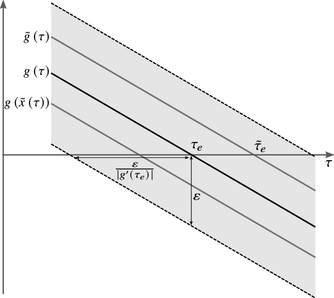
Figure 1: Estimating the uncertainty on the determination of a zero of an event function in the linear approximation. The exact event function $g\left(\tau\right)$ has a zero for $\tau=\tau_{e}$. Event detection is however performed on the truncated Taylor series of the event function $\tilde{g}\left(\tau\right)$, yielding a value of $\tau=\tilde{\tau}_{e}\neq\tau_{e}$. The adaptive timestep deduction scheme ensures that $\left|g\left(\tau\right)-\tilde{g}\left(\tau\right)\right|<\varepsilon$ within the integration step, where $\varepsilon$ is the integrator tolerance. The value of the event function when the integration is restarted after the detection of an event is ${g}\left(\tilde{{x}}\left(\tilde{\tau}_{e}\right)\right)$. Both $\tilde{g}\left(\tau\right)$ and ${g}\left(\tilde{{x}}\left(\tau\right)\right)$ do not differ from $g\left(\tau\right)$ more than $\varepsilon$ in absolute value, and thus $\left|{g}\left(\tilde{{x}}\left(\tilde{\tau}_{e}\right)\right)\right|<2\varepsilon$. In the linear approximation around the zero of the event function, the uncertainty $\varepsilon$ on the vertical axis can be projected on the $\tau$ axis via the derivative of the event function, thus yielding an estimation of the time interval within which discontinuity sticking can occur.

After the detection of an event, the state of the system has to be propagated up to the detected event trigger time $\tilde{\tau}_{e}$. The problem of discontinuity sticking can emerge at this stage. Due to both floating-point rounding and to the nonzero error tolerance $\varepsilon$ of the integration scheme, the propagated state $\tilde{x}(\tilde{\tau}_{e})$ will not satisfy exactly the event equation (4). As a consequence, during the following timestep, the newly expanded event function may have a detectable root representing the same event again. This potentially leads to cases where a never-ending loop of re-detection of the same event (discontinuity sticking) is created.

In mathematical terms, the value of the event function at the beginning of the following timestep is ${g}\left(\tilde{{x}}\left(\tilde{\tau}_{e}\right)\right)$ (because we used the truncated Taylor series $\tilde{{x}}\left(\tau\right)$ to propagate the state of the system). Because both $\tilde{g}\left(\tau\right)$ and ${g}\left(\tilde{{x}}\left(\tilde{\tau}\right)\right)$ are approximations of $g\left(\tau\right)$ with an accuracy of order $\varepsilon$ (see the pictorial sketch in Figure 1), we can then infer that

$$\left|{g}\left(\tilde{{x}}\left(\tilde{\tau}_{e}\right)\right)\right|<2\varepsilon.$$ (16)

It is now easy to see how, in the linear approximation around the zero of the event function, we can formulate an estimation of the time interval $\Delta\tau_{d}$ within which discontinuity sticking can occur (see Figure 1):

$$\Delta\tau_{d}<\frac{2\varepsilon}{\left|{g}^{\prime}\left(\tau_{e}\right)\right|}.$$ (17)

Note that the exact value of ${g}^{\prime}\left(\tau_{e}\right)$ is not known during the integration, however it is approximated to accuracy $\sim\varepsilon$ by $\tilde{g}^{\prime}\left(\tilde{\tau}_{e}\right)$. We can then quantify the relative error we commit when estimating $\Delta\tau_{d}$ via $\tilde{g}^{\prime}$ rather than ${g}^{\prime}$:

$$\frac{\frac{2\varepsilon}{{g}^{\prime}}-\frac{2\varepsilon}{{g}^{\prime}+\varepsilon}}{\frac{2\varepsilon}{{g}^{\prime}}}=\frac{\varepsilon}{{g}^{\prime}+\varepsilon}.$$ (18)

Thus, in the common case $\varepsilon\ll{g}^{\prime}$, the relative error is $\varepsilon/{g}^{\prime}$, while in the extreme case $\varepsilon\gg{g}^{\prime}$ the relative error on $\Delta\tau_{d}$ is $\sim 1$. Thus, we can add an extra factor $\times 2$ to the estimate (17) as an additional safety margin.

In heyoka, whenever a terminal event triggers, it enters a cooldown period of time within which the event is not allowed to trigger again. By default the cooldown value is computed via eq. (17), but the user can override the deduction logic by providing an explicit value for the cooldown (including zero). In §5.4, we will show how the cooldown mechanism is effective in dealing with the issue of discontinuity sticking.

5 Tests and examples

5.1 The Hénon & Heiles lost integral

As a first example, to test and validate heyoka’s event detection machinery, we will reproduce here a famous numerical experiment by Hénon & Heiles (1964) investigating the existence of a third integral of motion in axisymmetric potentials. On the basis of early numerical experiments and theoretical analyses (e.g., see Contopoulos (1963)), it was conjectured that axisymmetric potentials feature an additional integral of motion (beside the energy and the angular momentum integral), thus implying the Liouville-integrability of all axisymmetric systems (including, e.g., cubic galactic potentials).

In their analysis, Hénon & Heiles (1964) consider the autonomous Hamiltonian system

$$\mathcal{H}\left(\dot{x},\dot{y},x,y\right)=\frac{1}{2}\left(\dot{x}^{2}+\dot{y}^{2}\right)+U\left(x,y\right),$$ (19)

where the potential $U\left(x,y\right)$ is defined as

$$U\left(x,y\right)=\frac{1}{2}\left(x^{2}+y^{2}+2x^{2}y-\frac{2}{3}y^{3}\right).$$ (20)

$x$ and $y$ are the cylindrical coordinates of a point mass moving under the influence of the axisymmetric potential $U\left(x,y\right)$. The angular momentum integral of motion has already been eliminated in (19) via the introduction of cylindrical coordinates, and thus we are left with a two degrees of freedom system featuring one known integral of motion (the Hamiltonian itself).

For a given energy level $\mathcal{H}$, eq. (19) imposes the following constraint:

$$\frac{1}{2}\dot{x}^{2}=\mathcal{H}-U\left(x,y\right)-\frac{1}{2}\dot{y}^{2}\geq 0,$$ (21)

as $\frac{1}{2}\dot{x}^{2}$ cannot assume negative values. The inequality (21) defines a volume in the 3D phase space $\left(x,y,\dot{y}\right)$. On the other hand, if another integral of motion $\mathcal{C}=\mathcal{C}\left(\dot{x},\dot{y},x,y\right)$ exists, we can invert it to determine $\dot{x}=\dot{x}\left(x,y,\dot{y},\mathcal{C}\right)$, plug this definition of $\dot{x}$ into eq. (19) and obtain an equation of type

$$f\left(x,y,\dot{y},\mathcal{H},\mathcal{C}\right)=0.$$ (22)

Eq. (22) defines a surface embedded in the 3D phase space $\left(x,y,\dot{y}\right)$, rather than a volume. Thus, Hénon & Heiles (1964) propose the use of Poincaré sections (Teschl, 2012) to investigate the existence of $\mathcal{C}$: if $\mathcal{C}$ exists, then the Poincaré sections will consist of closed curves, otherwise they will resemble densely-filled surfaces.

Following Hénon & Heiles (1964), for the computation of Poincaré sections we consider the intersections of the solutions of (19) with the $\left(y,\dot{y}\right)$ plane in the 3D phase space $\left(x,y,\dot{y}\right)$, and we consider only intersections for which $\dot{x}>0$ (i.e., the particle is moving from below to above the plane). The intersection of a solution with the $\left(y,\dot{y}\right)$ plane can be detected in heyoka via the trivial event equation

$$x=0.$$ (23)

When a zero of the event function is detected, the values of $y$ and $\dot{y}$ at the intersection time are then determined via the dense output provided by the Taylor series of the solution and added to the Poincaré section.

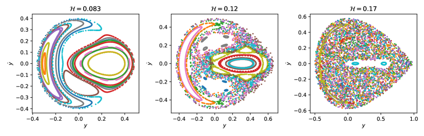
Figure 2: Poincaré sections on the $\left(y,\dot{y}\right)$ plane for the axisymmetric potential studied by Hénon & Heiles (1964) (see §5.1). Three energy levels $\mathcal{H}$ are considered. The Poincaré section for the lowest energy level $\mathcal{H}=0.083$ (left panel) consists of closed curves and would thus seem to indicate the existence of an additional integral of motion (beside the energy). However, as the energy level increases (center panel), regions of chaotic motion start to appear. Eventually, at the highest energy level (right panel) chaotic motion dominates the portrait, thus indicating that the additional integral of motion does not exist.

The Poincaré sections for the three energy levels considered by Hénon & Heiles (1964) are visualised in Fig. 2. Whereas at low energy levels the Poincaré section indeed resembles a collection of closed curves, as the energy level increases chaotic regions start to appear, and eventually dominate the portrait at the highest energy level. These numerical results led Hénon & Heiles (1964) to conclude that no additional integrals of motion exist in general for axisymmetric potentials, thus giving a negative answer to earlier conjectures.

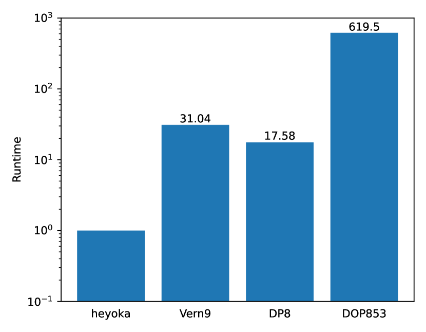
Figure 3: Runtime performance for the computation of a Poincaré section in the Hénon-Heiles dynamical system described in §5.1. The vertical axis shows the time required by several numerical integration libraries to compute the same Poincaré section, normalised by the timing for our Taylor integrator heyoka. heyoka is compared to the explicit Runge-Kutta schemes Vern9 and DP8 from DifferentialEquations.jl (Rackauckas & Nie, 2017) and DOP853 from SciPy (Virtanen et al., 2020), which support event detection via the sign change method. The error tolerance is set to $10^{-15}$ for all integrators. The timings were taken on an AMD Ryzen 3950X CPU.

From the performance point of view, we report in Figure 3 a runtime comparison between heyoka, the Vern9 and DP8 integrators from DifferentialEquations.jl (Rackauckas & Nie, 2017), and the DOP853 integrator from SciPy (Virtanen et al., 2020). The DP8 and DOP853 integrators are implementations of the explicit Dormand-Prince Runge-Kutta 8/5/3 method (Hairer et al., 1993), while Vern9 is a ninth-order explicit Runge-Kutta scheme (Verner, 2014). Apart from heyoka, all integrators employ the sign change method for event detection.

In this simple test, we can see how heyoka performs considerably better than the other integrators, being more than an order of magnitude faster than the integrators from DifferentialEquations.jl and more than two orders of magnitude faster than the SciPy integrator. Regarding the SciPy integrator, we should emphasise that its performance in this test is penalised by the slowness of the Python interpreter. Another performance comparison with DOP853 will be presented in §5.4, where DOP853 performs significantly better thanks to the fact that the evaluation of the right-hand side of the ODEs is mostly done in compiled C code (rather than in interpreted Python code).

5.2 Collision detection in the outer Solar System

In this test, we will be considering the long-term dynamics of the outer Solar System while keeping track of possible collisions between the planets. The dynamical system is set up as a gravitational 6-body problem consisting of the Sun, Jupiter, Saturn, Uranus, Neptune and Pluto, with initial conditions taken from Applegate et al. (1986). This dynamical system does not experience close encounters (let alone collisions) between the planets over a timespan of (at least) $10^{6}\,y$.

Collision detection is implemented with 15 event equations of the form

$$\left(x_{i}-x_{j}\right)^{2}+\left(y_{i}-y_{j}\right)^{2}+\left(z_{i}-z_{j}\right)^{2}-\left(2R\right)^{2}=0,$$ (24)

where $\left(x_{i},y_{i},z_{i}\right)$ and $\left(x_{j},y_{j},z_{j}\right)$ are the Cartesian coordinates of the $i$-th and $j$-th body respectively, and $R$ is the planetary radius, which, for simplicity, is assumed to be Jupiter’s radius for all bodies. The event equation (24) is satisfied when two planets (represented as spheres of radius $R$) come into contact. The error tolerance $\varepsilon$ in this numerical experiment is set to $10^{-18}$: as shown in Biscani & Izzo (2021), an error tolerance below machine epsilon ($\sim 10^{-16}$) allows our Taylor integrator to satisfy Brouwer’s law for the conservation of prime integrals over billions of dynamical timescales.

The purpose of this test is dual:

• first, we want to measure the overhead of event detection in a situation where no event ever triggers;

• second, we want to verify the claims made §3.2 and §3.3 about the optimality of our root isolation approach. Specifically, we want to verify experimentally that the fast exclusion check described in §3.3 is effective at quickly excluding the occurrence of events.

The CPU timings for a total integration time of $10^{6}\,\textnormal{y}$ are visualised in Figure 4, where we also included the timing for IAS15 (Rein & Spiegel, 2015). Like heyoka, IAS15 is a non-symplectic N-body integrator which is nevertheless able to satisfy Brouwer’s law over billions of dynamical timescales while at the same time resolving accurately the dynamics of close encounters. IAS15 supports collision detection via the usual approach of checking for sphere-sphere overlaps at the beginning of each timestep. Although this method is very cheap computationally, it cannot guarantee that collisions are not missed.

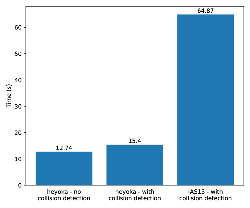
Figure 4: CPU timings for a $10^{6}\,\textnormal{y}$ integration of the outer Solar System (see §5.2). Our Taylor integrator, heyoka, is benchmarked with and without collision detection. The timing for the IAS15 integrator from REBOUND are also included. Collision detection in heyoka results in a $\sim 20\%$ slowdown with respect to an integration without collision detection. The timings were taken on an Intel Xeon Platinum 8360Y.

The timings for heyoka show how the overall performance overhead of event detection is $\sim 20\%$ for this test. Regarding the behaviour of the root-finding algorithm, in this test the fast exclusion check described in §3.3 was always able to exclude the triggering of collision events with no false positives.

5.3 Collisions and close encounters between planetary embryos

Whereas in the previous test (§5.2) we examined a non-collisional N-body system, in this example we will test the behaviour of our event detection approach in an N-body system characterised by frequent collisions and close encounters.

Collisional planetary systems play an important role in the study of the origin and evolution of the Solar System. Current theories of planet formation posit that planetary embryos form via the collision of kilometer-sized planetesimals, which in turn originate from the aggregation of dust in protoplanetary disks (Klahr & Schreiber, 2020). Planetary embryos have masses of about $10^{22}$ to $10^{23}\,\textnormal{kg}$, and they have diameters up to a few thousand kilometers. Over time, planetary embryos collide and merge with each other, eventually resulting in the formation of planets.

Numerical studies of planet formation (e.g., in the context of population synthesis, see Mordasini et al. (2009)) often employ hybrid integrators such as MERCURY (Chambers & Migliorini, 1997) or the closely-related MERCURIUS (Rein & Liu, 2012). Hybrid integrators consist of a symplectic integration scheme paired to a non-symplectic, high-accuracy integrator. The symplectic integrator is employed as long as the planets are not experiencing close encounters. When a close encounter is detected, the hybrid integrator switches to the high-accuracy scheme, resolves the encounter and finally resumes the simulation with the symplectic integrator. Note that although it is certainly possible to pair a Taylor integrator to a symplectic integrator to obtain a new type of hybrid integrator, in this example we will use heyoka to integrate both long-term dynamics and close encounters (i.e., without switches to other integration schemes).

Inspired by a numerical experiment outlined in Chambers (1999), we set up a gravitational N-body system consisting of the Sun and 30 planetary embryos with masses ranging between $0.2$ Earth masses and $0.6$ Lunar masses. The planetary embryos are placed on randomly-generated low-eccentricity and low-inclination orbits between $0.5\,\textnormal{AU}$ and $1.2\,\textnormal{AU}$. We follow the evolution of this dynamical system for $10^{4}$ years, and we keep track of both collisions and close encounters between the embryos. Collisions are detected via event equations like (24). For the detection of close encounters we use the event equation

$$\frac{1}{2}\frac{d\left(\boldsymbol{x}_{i}-\boldsymbol{x}_{j}\right)^{2}}{dt}=\left(x_{i}-x_{j}\right)\left(v_{xi}-v_{xj}\right)\\ +\left(y_{i}-y_{j}\right)\left(v_{yi}-v_{yj}\right)+\left(z_{i}-z_{j}\right)\left(v_{zi}-v_{zj}\right)=0,$$ (25)

which will be satisfied when the mutual distance between embryos $i$ and $j$ is at a stationary point. In order to filter out distance maxima, we impose the additional requirement that the direction of the event (i.e., the time derivative of the left-hand side of the event equation) must be positive, so that only distance minima are detected.

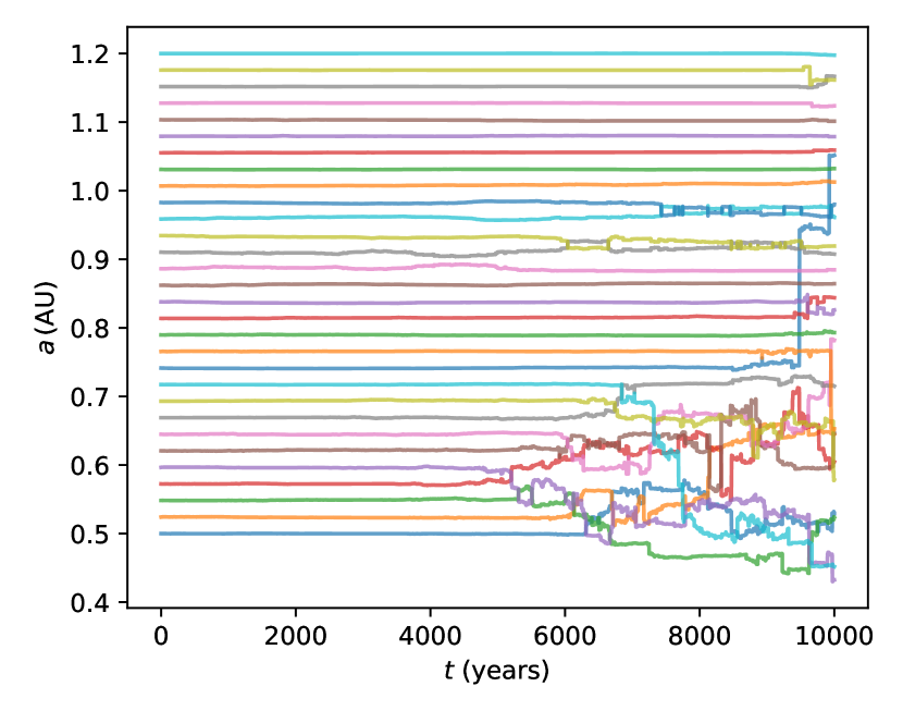
Figure 5: Evolution in time of the semi-major axes of 30 planetary embryos orbiting the Sun (see §5.3). The embryos are initially placed on quasi-circular quasi-planar orbits between $0.5\,\textnormal{AU}$ and $1.2\,\textnormal{AU}$. The chaotic gravitational interactions between the embryos eventually lead to close encounters and collisions.

The chaotic nature of this system is evident in the time evolution of the semi-major axes of the embryos (Figure 5). Our event detection algorithm detected a total of 31 planetary collisions within the $10^{4}$ years timespan. The cumulative number of close encounters between the embryos as a function of the encounter distance is visualised in Figure 5, with the closest planetary encounter taking place at a mutual distance of $\sim 2.8\,\textnormal{km}$. These results are in good agreement with the results from Chambers (1999).

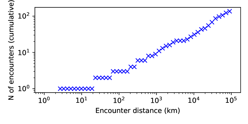
Figure 6: Cumulative number of close encounters between planetary embryos in the inner Solar System as a function of the encounter distance in the setup described in §5.3. The total simulation time is $10^{4}$ years.

Regarding the performance of the polynomial root finding algorithm in this test, like in the previous example (§5.2) the fast exclusion check described in §3.3 never resulted in false positives. When events did trigger, the polynomial root isolation procedure always terminated in a single iteration. That is, the CA algorithm immediately detected a single sign change in the coefficients of the transformed polynomial, thereby determining that a single event would trigger within the timestep. Thus, like in §5.2, we conclude that our experiments indicate that the polynomial root finding algorithm is behaving in the optimal way also in collisional planetary N-body simulations.

We need to emphasise that our goal in presenting this test is not necessarily to advocate for the use of heyoka in all simulations of this kind. When the collisional dynamics matters only statistically, the risk of missing a single collision is acceptable and existing hybrid integrators may be able to simulate the system more efficiently. We do believe though, also in those cases, that the event detection guarantees provided by heyoka (coupled to its abilities to respect Brouwer’s law in long-term integrations and to accurately resolve close encounters via its adaptive timestepping scheme) are useful to measure the magnitude of the effects introduced by allowing planetary collisions to be missed.

5.4 Eclipsed trajectories around irregular bodies

In this last example, we consider the motion of a test mass around an irregular body, subject to the gravity and to the solar radiation acceleration, accounting for possible eclipses. Such a problem is relevant for the study of the long term stability of spacecraft orbits around asteroids and comets (as most recently argued by Lang (2021)), as well as for the accurate prediction of possible ejecta from active asteroids such as the documented case of the asteroid Bennu (Chesley et al., 2020).

Let us model the asteroid gravity using a mascon model. Mascon models are known to be appropriate to describe the gravity of small irregular bodies where they have the advantage of being computationally efficient (Wittick & Russell, 2017) and able to represent also non homogeneous bodies (Park et al., 2010). We indicate with $N$ the number of mascons, with $m_{j}$ their masses and with $\mathbf{r}_{j}$ their position. Our reference frame is attached to the body, assumed to be in a uniform rotation with an angular velocity $\boldsymbol{\omega}$. Hence Coriolis and centrifugal accelerations need to be accounted for. We model the solar radiation pressure introducing an acceleration $\eta$ acting against the Sun direction $\hat{\mathbf{i}}_{S}$ and regulated by the eclipse factor $\nu(\mathbf{r})\in[0,1]$ which determines the eclipse-light-penumbra regime. In particular, $\nu=1$ when the body is fully illuminated, $\nu=0$ when fully eclipsed (umbra). Formally, the following set of differential equations are considered:

$$\ddot{\mathbf{r}}=-G\sum_{j=0}^{N}\frac{m_{j}}{|\mathbf{r}-\mathbf{r}_{j}|^{3}}(\mathbf{r}-\mathbf{r}_{j})-2\boldsymbol{\omega}\times\mathbf{v}-\boldsymbol{\omega}\times\boldsymbol{\omega}\times\mathbf{r}-\eta\nu(\mathbf{r})\hat{\mathbf{i}}_{S}(t),$$ (26)

where the Sun direction $\hat{\mathbf{i}}_{S}(t)=\mathbf{R}(t)\hat{\mathbf{i}}_{S}(0)$ is modelled, neglecting the asteroid orbital motion, rotating the initial Sun direction $\hat{\mathbf{i}}_{S}(0)$ around the asteroid rotation axis, of an angle $\omega t$. The eclipse factor $\nu(\mathbf{r})$ in the above equation adds quite some complexity to the dynamics.

Let us neglect here the penumbra regime and assume $\nu$ switches instantaneously between extreme values whenever the center of mass enters into the shadowed region created by a point source Sun. The resulting dynamical system is then a hybrid system switching dynamical regimes according to whether the spacecraft is subject or not to the solar radiation acceleration. In order to detect such a switch condition and be able to use the event detection machinery of any initial value solver, we introduce a function changing sign when entering/exiting eclipsed areas. The eclipse function $F(\mathbf{r},\hat{\mathbf{i}}_{S})$ is defined as the distance of $\mathbf{r}$ from the shadow cone (degenerated into a cylinder in this case) cast by the body along the $\hat{\mathbf{i}}_{S}$ direction, if $\mathbf{r}$ is outside the cone. Whenever $\mathbf{r}$ is inside the eclipsed portion of the space around the irregular body, the eclipse function is defined as the length of the segments belonging to the ray passing through $\mathbf{r}$ that are inside the body, transformed into a negative number. We have built a function whose zero level curve, fixing any direction, describes the border of the eclipsed area and can be thus detected as an event and used to propagate the hybrid system.

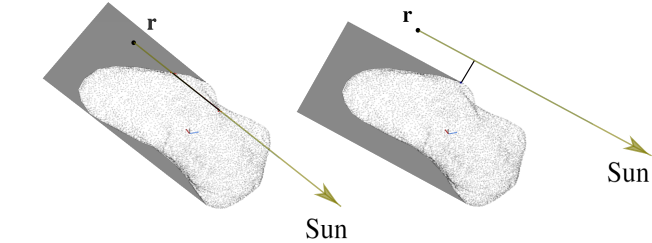
Figure 7: Definition of the eclipse function $F(\mathbf{r},\hat{\mathbf{i}}_{S})$ (black segment) in the case of the asteroid Eros. The eclipse function is defined as a positive number outside of the eclipse cone (right). Inside the eclipse cone (left) is a negative number whose magnitude is the length of the ray inside the body.

In Figure 7, a visualization of the eclipse function $F$ is reported.

Assuming a shape model is available for the irregular body, its three dimensional surface triangular mesh can be used to compute the numerical value of the eclipse function by applying, for example, the Möller-Trumbore algorithm (Möller & Trumbore, 1997) to the ray originating in $\mathbf{r}$ and directed as $\hat{\mathbf{i}}_{S}$. An alternative approach to compute the eclipse function would be to use ray marching Sherstyuk (1999) and rely on a distance function computed from the available surface triangular mesh. These approaches to computing the eclipse function have two main drawbacks. Firstly, they can be computational expensive. Depending on the accuracy of the shape model, the number of triangles in the mesh is typically high, and even for a relatively low precision model, anyway in the order of thousands. The computation of the eclipse function is to be done at each time step of the numerical integration and therefore adds up directly to the computational complexity of a single integration step. Secondly, nor the Möller-Trumbore algorithm nor the ray marching approach are differentiable to an arbitrary order: if we are to take advantage of the properties of the proposed event detection method in a Taylor integration scheme, the event function needs to have this property. For this purpose we represent the eclipse function with a feedforward artificial neural network relying on its universal function approximator property (Calin, 2020). The purpose of this test is thus threefold:

• first, we want show the use of heyoka in cases where the event equations and/or the dynamical equations contain a deep network. The highly recursive nature of deep networks allows the just-in-time compilation to happen efficiently even if the explicit mathematical expressions involved are not manageable;

• second, we want to show a practical case where the use of a reliable event detection machinery makes a significant difference on the precision of the obtained results;

• third, we want to verify the claims made §4.3 on the discontinuity sticking problem.

The use of deep networks to construct three dimensional differentiable representations of complex objects has been demonstrated by a number of recent works (Mildenhall et al., 2020; Park et al., 2019; Izzo & Gómez, 2021; Derksen & Izzo, 2021) and is often referred to as implicit neural representation. The eclipse function we here introduced, is similar to the signed distance function used by Park et al. (2019) to learn implicit neural representations of objects. Here we do not discuss in detail the generic network architecture employed, its training and performances which are, instead, the subject of a future separated work. For the purpose of this paper we use one of such networks $\mathcal{N}$, that we call eclipseNet, trained to approximate the eclipse function over the shape model of the asteroid Eros taken from the work of Gaskell (2008) and reduced to 14744 triangles for convenience. At the end of the training the average mean square error obtained for this particular eclipseNet translates to less than 1% relative error on the prediction of the zeros of the eclipse function, and a three orders of magnitude speed up with respect to the approach based on the Möller-Trumbore algorithm. The resulting eclipse function is fully differentiable (the network non-linearities used are hyperbolic tangents) at arbitrary order, so that it is possible to compute, along any trajectory solution to eq. (26), the quantities

$$\frac{d^{n}F}{dt^{n}}=\frac{d^{n}\mathcal{N}(\mathbf{r}(t),\hat{\mathbf{i}}_{S}(t))}{dt^{n}},$$

exploiting the automated differentiation machinery of the Taylor integrator.

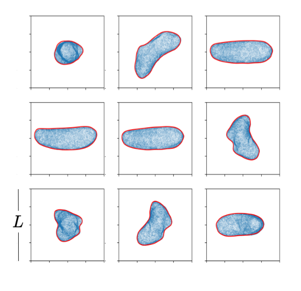
Figure 8: Visualization of the eclipseNet inference over 9 different Sun directions unseen during training. The red line represents the zero level curve of the eclipseNet which is to be detected by the event machinery signalling the entrance (or exit) into the asteroid shadow cone. In blue we report the vertices of the shape model for Eros projected onto the view plane. Length units are $L=19.52$ km

To get a visual glimpse on the learned differentiable version of the eclipse function, we visualize, in Figure 8, the network predictions from nine random views $\hat{\mathbf{i}}_{S}$ not encountered during the training. In other words, the network was never exposed to any of these data during training and yet is able to reproduce consistently to good detail the eclipse function next to its zero.

We now move on and consider again the initial value problem for eq. (26) where the eclipse factor $\nu$ switches between its two extreme values in correspondence to the roots of the event equation defined by the eclipseNet: $\mathcal{N}(\mathbf{r},\hat{\mathbf{i}}_{S})=0$. The sign of the event equation derivative will determine whether the spacecraft is entering (negative) or leaving (positive) the eclipse.

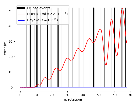
Figure 9: As Eros rotates and the orbit is propagated, a number of eclipse events are encountered. The effect of missing some of the events is here visualized in terms of the resulting error. As some early eclipses are missed by the event detection based on a 8th order Dormand-Prince, the resulting error grows invalidating the outcome. On the other hand, heyoka’s event detection keeps the usual Taylor integration accuracy through the various eclipse events.

We solve the same initial value problems using our Taylor integrator heyoka (where the switching of $\nu$ between the extremal values is implemented in the callback of a terminal event, see §4.2), and a standard Dormand-Prince 8th order numerical integrator (DOP853) from SciPy (Virtanen et al., 2020) using a sign based event detection. Like most modern packages for event detection, DOP853 only monitors the sign of the event function along the numerical propagation searching for a change in its value as computed at two subsequent timesteps. Upon triggering of such a condition a root finding method is deployed in that interval to find and return the zero of the event function. It is important to note here that solvers choose their adaptive step size so as to compute the dynamics accurately, without accounting for the event function variations (Shampine & Thompson, 2000). As a consequence, there is no way to know if events are lost along the propagation and one is often left to hope that setting the accuracy to the maximum possible value the likelihood of significant event being lost is small if not vanishing.

In our tests, we set the accuracy of the Dormand-Prince numerical integrator, both in terms of absolute and relative tolerances, to the highest level allowed (100 times the machine epsilon), so that the chances to lose events are minimized. We perform simulations first without tracking events and then activating the event machinery and thus simulating also the eclipsed dynamics. We propagate the same initial conditions in different setups and use non dimensional units setting the Cavendish constant to one, using $L=19.52$ km as length unit and $M=6.687\cdot 10^{15}$ kg as mass unit. The initial conditions simulated are $\mathbf{r}_{0}=[0,3,0],\mathbf{v}_{0}=[-\sqrt{3}/3\cos i+3\omega,0,\sqrt{3}/3\sin i]$, where $i$ is the initial inclination here set to $21^{\circ}$ and $\omega$ is set to . Different choices of the initial conditions return similar results as far as they allow for eclipses to be present. The integration time is set to $T=100\pi$.

The results are reported in Table 1, where the different setups are compared in terms of CPU time and precision achieved. The maximum error reported refers to the position and is computed with respect to a ground truth generated by propagating the same system of differential equations using quadruple precision and the reliable event detection approach here introduced. In Figure 10 we visualize the resulting orbit when eclipse events are reliably tracked.

Table 1: Speed and precision achieved for several setups in the integration of eclipsed trajectories around irregular bodies (see §5.4). When eclipse events need to be tracked DOP853 is faster as it ignores the event equation in its adaptive stepper, thus taking larger steps at the price of missing out entire eclipse events.

	CPU time	Max. Error (position)
without eclipse events
heyoka ($\epsilon=10^{-16}$)	4.64s	2.44e-14
heyoka ($\epsilon=10^{-13}$)	2.85s	1.49e-11
DOP853 (tol$=2.2\cdot 10^{-14}$)	8.5s	5.26e-11
with eclipse events
heyoka ($\epsilon=10^{-16}$)	35.85s	1.23e-14
DOP853 (tol$=2.2\cdot 10^{-14}$)	6.57s	1.32e-02

The numerical propagations without eclipse events confirm, as reported already by Biscani & Izzo (2021), that the Taylor integration scheme achieves great precision and CPU timings outperforming DOP853. When eclipse event need to be tracked DOP853 becomes faster as it ignores the event equation in its adaptive stepper, thus taking larger steps at the price of missing out entire eclipse events. The consequences on the integration error are significant with ten orders of magnitude lost as eclipse events are missed. The reliable event machinery proposed in this paper and implemented in the Taylor integrator in heyoka, is instead able to adaptively choose the step size as to follow also the event function with he necessary accuracy. This can slow down the integration, as more steps may be needed, but is a necessary and fair cost to pay to not introduce unacceptable errors (as explained in §4.1).

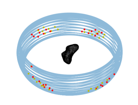
Figure 10: Simulated orbit around Eros. Points of entry into eclipse are indicated in red, while points of exit in yellow. Eclipses are encountered in different points around the orbit as the Sun moves in the asteroid reference frame.

Regarding the approach proposed in §4.3 for the handling of discontinuity sticking via automatic cooldown deduction in terminal events, our testing confirmed that all terminal events in heyoka for this test triggered exactly once. Removing the automatic cooldown deduction heuristic also confirmed that the eclipse crossing events often triggered multiple times in rapid succession, due to the discontinuity sticking phenomenon (although they never led to an endless loop of re-detection of the same event). By contrast, in this test the DOP853 integrator would routinely get stuck in an infinite loop of re-detection of the eclipse crossing events, leading to the need to implement a workaround involving the redefinition of the dynamical system at each eclipse crossing and the manual specification of alternating directions for the event.

6 Caveats and limitations

Despite the fact that our tests and numerical experiments indicate that our approach for the detection of events in Taylor integrators via real-root isolation is both efficient and reliable, we need to point out a couple of caveats and limitations.

To begin with, our approach requires the event equations (4) to be formulated as differentiable mathematical expressions of the state variables (and, possibly, time). This is a limitation that stems directly from the very nature of Taylor integrators implemented on top of automatic differentiation, which cannot deal with non-differentiable expressions (such as, e.g., black box functions) in the definition of an ODE system. Such a limitation is though alleviated as the development of differentiable models approximating complex numerical algorithms (e.g., used to write the r.h.s. of the equations to be integrated) is often possible training, for example, artificial neural networks models as hinted in Section §5.4.

Secondly, like most polynomial root-finding procedures, the real-root isolation process described in §3 breaks down in correspondence of roots of multiplicity greater than one. As pointed out by Park & Barton (1996), it is in general exceedingly unlikely for the high-order polynomials generated during a numerical integration to feature repeated roots (especially when using floating-point arithmetic). Badly-conditioned event equations can, however, always lead to repeated roots in the Taylor series expansions. For instance, an event equation of the type

$$\left[g\left(t,\boldsymbol{x}\left(t\right)\right)\right]^{2}=0$$ (27)

will be troublesome, because both the event function and its time derivative will be zero when the event triggers. This will translate to a Taylor series with a double root in correspondence of the event trigger time, which, at best, will result in reduced performance and, at worst, in missing events altogether. Additionally, in case of terminal events the automatically-deduced cooldown value in correspondence of a double root will tend to infinity (see §4.3). Thus, as a general rule, event functions in which the event trigger times are stationary points are to be avoided.

7 Conclusions

In this paper we introduced a novel, reliable approach for event detection in the numerical solution of ordinary differential equations via Taylor’s method. Our method is based on the construction of high-order polynomial approximations of the event functions, whose roots are located via the Collins-Akritas real-root isolation scheme. Leveraging the availability of free dense output in Taylor’s integration method, our approach is computationally cheap while at the same time offering strong event detection guarantees.

We have tested the implementation of the new algorithm in our open source numerical integration package heyoka on several astrodynamical problems of interest, such as collisional N-body systems, spacecraft dynamics around irregular bodies accounting for eclipses and the computation of Poincaré sections. In all cases the reliable event detection mechanism here proposed, coupled with the known properties of Taylor methods, produces results that are a significant improvement over the currently available alternatives.

Our work fills a gap in the capabilities of modern astrodynamical numerical integration packages, which typically do not feature builtin event detection capabilities. We hope that our work will be useful to practitioners and researchers, and that it will stimulate and enable further research and advances in computational celestial mechanics.

Data Availability

No new data were generated or analysed in support of this research.

The source code of the software described in the paper is freely available under an open source license at the repositories https://github.com/bluescarni/heyoka and https://github.com/bluescarni/heyoka.py.

References

- Aberth (1973) Aberth O., 1973, Mathematics of computation, 27, 339
- Agol et al. (2021) Agol E., Hernandez D. M., Langford Z., 2021, Monthly Notices of the Royal Astronomical Society, 507, 1582
- Alefeld et al. (1995) Alefeld G., Potra F. A., Shi Y., 1995, ACM Transactions on Mathematical Software (TOMS), 21, 327
- Applegate et al. (1986) Applegate J. H., Douglas M. R., Gürsel Y., Sussman G. J., Wisdom J., 1986, in Hut P., McMillan S. L. W., eds, The Use of Supercomputers in Stellar Dynamics. Springer Berlin Heidelberg, Berlin, Heidelberg, pp 96–114
- Benner & Sawyer (1973) Benner M. S., Sawyer R. H., 1973, NASA Special Publication, 3082
- Biscani & Izzo (2021) Biscani F., Izzo D., 2021, Monthly Notices of the Royal Astronomical Society, 504, 2614
- Branicky (2005) Branicky M. S., 2005, Introduction to Hybrid Systems. Birkhäuser Boston, Boston, MA, pp 91–116, doi:10.1007/0-8176-4404-0_5, https://doi.org/10.1007/0-8176-4404-0_5
- Budan (1807) Budan F.-D., 1807, Nouvelle méthode pour la résolution des équations numériques d’un degré quelconque: d’après laquelle toute le calcul exigé pour cette résolution se réduit à l’emploi des deux premières règles de l’arithmétique. Courcier
- Calin (2020) Calin O., 2020, in , Deep Learning Architectures. Springer, pp 251–284
- Chambers (1999) Chambers J. E., 1999, Monthly Notices of the Royal Astronomical Society, 304, 793
- Chambers & Migliorini (1997) Chambers J. E., Migliorini F., 1997, in AAS/Division for Planetary Sciences Meeting Abstracts #29. p. 27.06
- Chesley et al. (2020) Chesley S., et al., 2020, Journal of Geophysical Research: Planets, 125, e2019JE006363
- Collins & Akritas (1976) Collins G. E., Akritas A. G., 1976, in Proceedings of the third ACM symposium on Symbolic and algebraic computation. pp 272–275
- Contopoulos (1963) Contopoulos G., 1963, The astronomical journal, 68, 1
- Derksen & Izzo (2021) Derksen D., Izzo D., 2021, in Proceedings of the IEEE/CVF Conference on Computer Vision and Pattern Recognition. pp 1152–1161
- Gaskell (2008) Gaskell R., 2008, Eros polyhedral model
- Grabner et al. (2003) Grabner G., Kittinger R., Kecskeméthy A., 2003, IFAC Proceedings Volumes, 36, 251
- Hairer et al. (1993) Hairer E., Nørsett S. P., Wanner G., 1993, Solving ordinary differential equations. 1, Nonstiff problems. Springer-Vlg
- Hénon & Heiles (1964) Hénon M., Heiles C., 1964, The astronomical journal, 69, 73
- Izidoro et al. (2017) Izidoro A., Ogihara M., Raymond S. N., Morbidelli A., Pierens A., Bitsch B., Cossou C., Hersant F., 2017, Monthly Notices of the Royal Astronomical Society, 470, 1750
- Izzo & Gómez (2021) Izzo D., Gómez P., 2021, arXiv preprint arXiv:2105.13031
- Jorba & Zou (2005) Jorba À., Zou M., 2005, Experimental Mathematics, 14, 99
- Karlsson (2005) Karlsson B., 2005, Beyond the C++ standard library: an introduction to boost. Pearson Education
- Kerner (1966) Kerner I. O., 1966, Numerische Mathematik, 8, 290
- Klahr & Schreiber (2020) Klahr H., Schreiber A., 2020, The Astrophysical Journal, 901, 54
- Kobel et al. (2016) Kobel A., Rouillier F., Sagraloff M., 2016, in Proceedings of the ACM on International Symposium on Symbolic and Algebraic Computation. pp 303–310
- Lang (2021) Lang A., 2021, Acta Astronautica, 182, 251
- Mao & Petzold (2002) Mao G., Petzold L. R., 2002, Computers & Mathematics with Applications, 43, 65
- Mildenhall et al. (2020) Mildenhall B., Srinivasan P. P., Tancik M., Barron J. T., Ramamoorthi R., Ng R., 2020, in European conference on computer vision. pp 405–421
- Möller & Trumbore (1997) Möller T., Trumbore B., 1997, Journal of graphics tools, 2, 21
- Mordasini et al. (2009) Mordasini C., Alibert Y., Benz W., 2009, Astronomy & Astrophysics, 501, 1139
- Neumaier (1990) Neumaier A., 1990, Interval methods for systems of equations. Cambridge university press
- Obreschkoff (1963) Obreschkoff N., 1963, Verteilung und berechnung der Nullstellen reeller Polynome. VEB Deutscher Verlag der Wissenschaften
- Ostrowski (1950) Ostrowski A., 1950, Annals of Mathematics, pp 702–707
- Park & Barton (1996) Park T., Barton P. I., 1996, ACM Transactions on Modeling and Computer Simulation (TOMACS), 6, 137
- Park et al. (2010) Park R. S., Werner R. A., Bhaskaran S., 2010, Journal of guidance, control, and dynamics, 33, 212
- Park et al. (2019) Park J. J., Florence P., Straub J., Newcombe R., Lovegrove S., 2019, in Proceedings of the IEEE/CVF Conference on Computer Vision and Pattern Recognition. pp 165–174
- Rackauckas & Nie (2017) Rackauckas C., Nie Q., 2017, Journal of Open Research Software, 5
- Rein & Liu (2012) Rein H., Liu S.-F., 2012, Astronomy & Astrophysics, 537, A128
- Rein & Spiegel (2015) Rein H., Spiegel D. S., 2015, Monthly Notices of the Royal Astronomical Society, 446, 1424
- Sagraloff & Mehlhorn (2016) Sagraloff M., Mehlhorn K., 2016, Journal of Symbolic Computation, 73, 46
- Shampine & Reichelt (1997) Shampine L. F., Reichelt M. W., 1997, SIAM journal on scientific computing, 18, 1
- Shampine & Thompson (2000) Shampine L., Thompson S., 2000, Computers & Mathematics with Applications, 39, 43
- Shampine et al. (1991) Shampine L. F., Gladwell I., Brankin R. W., 1991, ACM Transactions on Mathematical Software (TOMS), 17, 11
- Sherstyuk (1999) Sherstyuk A., 1999, in Computer Graphics Forum. pp 139–147
- Sturm (2009) Sturm C., 2009, in , Collected Works of Charles François Sturm. Springer, pp 345–390
- Teschl (2012) Teschl G., 2012, Ordinary differential equations and dynamical systems. American Mathematical Soc.
- Verner (2014) Verner J. H., 2014, Numerical Algorithms, 65, 555
- Vincent (1836) Vincent A. J. H., 1836, Journal de Mathématiques Pures et Appliquées, 1, 341
- Virtanen et al. (2020) Virtanen P., et al., 2020, Nature Methods, 17, 261
- Wittick & Russell (2017) Wittick P. T., Russell R. P., 2017, in AAS/AIAA Astrodynamics Specialist Conference. pp 17–162