The Higgs boson as a self-similar system: A new solution to the hierarchy problem

Abstract

We propose a new solution to the hierarchy (naturalness) problem, concerning quantum corrections of the Higgs mass. Suggesting the Higgs boson as a system with a self-similar internal structure, we calculate its two-point function and find that the quadratic divergence is replaced by a logarithmic one. It is shown that the partonic-like distribution follows the Tsallis statistics and also high energy physics experimental data for the Higgs transverse momentum distribution can be described by a self-similar statistical model.

I Introduction

After the discovery of the Higgs boson with a mass around $125\,\mathrm{GeV}$ at the Large Hadron Collider (LHC), although the last piece of the Standard Model (SM) has been found ATLAS:2012yve ; CMS:2012qbp ; CMS:2013btf , some features of the Higgs boson are still under debate and investigation. Moreover, there are important issues, such as the mass of neutrinos, matter-antimatter asymmetry, dark matter and the hierarchy problem, which are left unanswered in the SM and should be addressed in a more fundamental theory. On the other hand, no significant deviations from the SM predictions have been observed so far at high energy collisions and the theory may be generalized to high energy scales. In this sense, the hierarchy problem of scales between the weak and higher energy scales is more evident when considering quantum fluctuations to calculate the Higgs squared mass corrections Veltman:1980mj

$$\delta m_{h}^{2}\sim\frac{\Lambda^{2}}{v^{2}}\left(m_{h}^{2}+2m_{W}^{2}+m_{Z}^{2}-4m_{t}^{2}\right),$$ (1)

where $\Lambda$ is the cutoff, the highest accessible energy scale, $v\simeq 246\,\mathrm{GeV}$ is the electroweak (EW) symmetry breaking scale and $m_{h}$, $m_{W,Z}$, and $m_{t}$ denote the mass of Higgs, gauge boson and top quark particles. Thus, if $\Lambda$ is very large, for instance as larger as the Planck mass, the corrections will be extremely greater than the Higgs mass value.

Theories beyond the SM may have an additional contribution to the Higgs mass such that it is finely adjusted to cancel $\delta m_{h}^{2}$. Supersymmetric models Draper:2016pys and composite Higgs scenarios Panico:2015jxa are such endeavors to avoid this problem. The fine-tuning in cancellation can be measured as

$$\Delta\geq\frac{\delta m_{h}^{2}}{m_{h}^{2}}\sim\left(\frac{\Lambda}{450\,\mathrm{GeV}}\right)^{2}.$$ (2)

Therefore, in these new theories, for $\Lambda\gg\mathrm{TeV}$, the Higgs boson mass cannot be found due to the cancellation.

In the SM, the Higgs boson is the only elementary scalar field and all other scalars are bound states of the strongly coupled sector. If the Higgs is also elaborated to be a composite bound state, it can be originated from a new strongly interacting dynamics, since Quantum Chromodynamics (QCD) cannot be responsible for its construction. That is the notion established in composite Higgs models Ahmadvand:2020izy , avoiding the hierarchy problem.

In this paper, the Higgs boson is considered as a complex system with an internal structure which reveals a statistical self-similarity behavior in that constituents are similar to the main system at a different level of scale.

Self-similar objects and patterns, known as fractals, have been widely studied in various areas of science including mathematics, biology and physics, as widely found in nature (not necessarily as exact fractals) Mandelbrot . In particle physics, especially in strong interactions, self-similar systems have been used to model hadrons which are composed of hadrons Hagedorn:1965st ; Frautschi:1971ij ; Chew:1971xwl . These models were able to describe many features of the hadronic system consistent with experimental data. Additionally, in high energy collision experiments of strong interactions, showing nearly scale invariant properties, the transverse momentum data would be well described in this context Bediaga:1999hv ; Cleymans:2011in ; Marques:2012px ; Deppman:2019yno if the Boltzmann-Gibbs statistics were replaced by the Tsallis statistics Tsallis:1987eu ; Curado:1991jc .

In the present work, we first obtain the two-point function of the Higgs with the self-similar internal structure, whose partonic-like distribution is described by the Tsallis statistics. We then show the modification of the field strength renormalization gives rise to the logarithmic divergence of the Higgs mass corrections. Note that the Higgs can be resulted from a new QCD-like dynamics at high energies and hence not only is the hierarchy problem addressed in this setup, but also the prediction of the Higgs mass is naturally feasible without restricting the given confining scale to be around the TeV.

II Correlation function

We now investigate the two-point correlation function of the Higgs, in accordance with the aforementioned considerations, for the interacting theory, $\langle\Omega|\phi(x)\phi(y)|\Omega\rangle$. Using a complete set of intermediate states at the scale level $n$

$$\mathbf{1}=\sum_{\psi_{n}}\int\frac{d^{3}p}{(2\pi)^{3}}\frac{1}{2E_{p}}|\psi_{n}\rangle\langle\psi_{n}|,$$ (3)

the two-point function for $x^{0}>y^{0}$ can be written as

$$\langle\Omega|\phi(x)\phi(y)|\Omega\rangle=\sum_{\psi_{n}}\int\frac{d^{3}p}{(2\pi)^{3}}\frac{1}{2E_{p}}\langle\Omega|\phi(x)|\psi_{n}\rangle\langle\psi_{n}|\phi(y)|\Omega\rangle,$$ (4)

where $E_{p}=\sqrt{\mathbf{p}^{2}+m^{2}}$ and $|\psi_{n}\rangle$ is the self-similar partonic state which can be an eigenstate of 4-momentum $P^{\mu}$. Because of translational invariance,

$$\langle\Omega|\phi(x)|\psi_{n}\rangle =\langle\Omega|\phi(0)|\psi_{n}\rangle\,e^{-ip.x}$$

$$\langle\psi_{n}|\phi(y)|\Omega\rangle =\langle\psi_{n}|\phi(0)|\Omega\rangle\,e^{ip.y},$$ (5)

thus Eq. (4) is expressed as

$$\langle\Omega|\phi(x)\phi(y)|\Omega\rangle=\sum_{\psi_{n}}\int\frac{d^{4}p}{(2\pi)^{4}}\frac{e^{-ip.(x-y)}}{p^{2}-m^{2}+i\epsilon}|\langle\Omega|\phi(0)|\psi_{n}\rangle|^{2}.$$ (6)

For $y^{0}>x^{0}$ the same procedure can be written to express the time-ordered product of the function. Furthermore, we can represent the scalar function as the K$\ddot{\mathrm{a}}$llen-Lehmann representation in terms of a spectral function

$$\langle\Omega|T\phi(x)\phi(y)|\Omega\rangle=\int_{0}^{\infty}\frac{dM^{2}}{(2\pi)}\rho(M^{2})\,D_{F}(x-y;M^{2}),$$ (7)

where $D_{F}$ is the Feynman propagator. Rewriting the effective state in terms of self-similar partonic constituent states

$$|\psi_{n}\rangle=\sum_{i}\langle\psi_{i}|\psi_{n}\rangle|\psi_{i}\rangle,$$ (8)

we can explore the effect of internal structure. In this case the spectral function of the main system will be

$$\rho(M^{2})\sim\sum_{i}(2\pi)\delta(M^{2}-m_{h}^{2})|\langle\Omega|\phi(0)|\psi_{i}\rangle|^{2}|\langle\psi_{i}|\psi_{n}\rangle|^{2}.$$ (9)

As a result, the two-point function becomes

$$\langle\Omega|T\phi(x)\phi(y)|\Omega\rangle\sim\sum_{i}\int_{0}^{\infty}dM^{2}\,\delta(M^{2}-m_{h}^{2})\,Z\,|\langle\psi_{i}|\psi_{n}\rangle|^{2}D_{F},$$ (10)

where $Z$ is effectively defined as the field strength renormalization and

$$|\langle\psi_{i}|\psi_{n}\rangle|^{2} =\sum_{i}\int d\Pi_{i}~{}|\mathcal{M}|^{2}$$

$$=\sum_{i}\bigg{(}\prod_{i}\int\frac{d^{4}p_{i}}{(2\pi)^{4}}\bigg{)}|\mathcal{M}_{0}|^{2}\,f\,(2\pi)^{4}\delta^{4}\left(\sum p_{i}-k\right).$$ (11)

Here, $\mathcal{M}$ is the probability amplitude of finding the subsystem $i$th of the system with mass $m_{i}$ as a fraction of $M$, $\mathcal{M}_{0}$ can be thought of as a scattering amplitude of the partonic system to $N$ constituent fields with a different energy level with respect to the system, and $f$ includes the contribution of substructures and determines the parton distribution function of the scale invariant parameter in the model. Hence, it is expected that $|\mathcal{M}_{0}|^{2}$ is proportional to the dimensional parameter of the system $M^{2}$ which is normalized to the energy scale of the larger system $E_{k}^{2}$, that is to say, the accessible energy of the intermediate state which can be probed, thereby we approximate it as $|\mathcal{M}_{0}|^{2}\sim M^{2}/E_{k}^{2}$. Now, one should find how this scale invariant parameter of the system, $x=M/E_{k}=m_{i}/M$, is distributed to partons through the distribution function.

Based on the Maxwell distribution for the ideal gas with $N$ particles,

$$f(K)=\mu^{-\frac{3N}{2}}K^{\frac{3N}{2}-1}e^{-\frac{K}{\mu}},$$ (12)

where $K=\mathbf{k}^{2}/(2M)$ and $\mu$ is proportional to the normalization factor, we try to obtain the distribution for a system having an internal energy and hence with a total energy $K+I=K(1+I/K)$ where $K$ stands for the kinetic energy of the system and $I$ for the internal energy. For the self-similar system, $I/K$ remains constant as the scale invariant parameter for all subsystems such that $I/K=I^{(n)}/K^{(n)}=x$. Due to the self-similarity feature, the energy distribution of internal subsystems should be equal at different levels and follow the main structure. Thus, taking the contribution of all subsystems into account, we consider the total energy $U$ of the system as follows

$$U=K\left(1+x\right)g(x)=K\left(1+x\right)^{\alpha},$$ (13)

where $\alpha$ denotes the fractal index and will be determined in the following by the relevant statistics of the system. From Eq. (13), $U\sim K+I\alpha(1+x)^{\alpha^{\prime}}$, and for this system with $f(U)=f(K)f(x)$ we can write

$$f(U) =\mu^{-\frac{3N}{2}}U^{\frac{3N}{2}-1}e^{-\frac{U}{\mu}}$$

$$=\mu^{-\frac{3N}{2}}K^{\frac{3N}{2}-1}\left(1+x\right)^{-\frac{3N}{2}\alpha-\alpha}e^{-\frac{K}{\mu}\left(1+x\right)^{\alpha}}.$$ (14)

Therefore, the integration over 3-momentum components of Eq. (II) for the distribution is obtained as

$$~{}~{}~{}~{}~{}\sum_{i}\bigg{(}\prod_{i}\int\frac{d^{3}p_{i}}{(2\pi)^{3}}e^{\frac{p_{i}^{2}}{2M}}f(x)\bigg{)}(2\pi)^{3}\delta^{3}\left(\sum\vec{p_{i}}-\mathbf{k}\right)$$

$$=\int dK\,\mu^{-\frac{3N}{2}}K^{\frac{3N}{2}-1}\left(1+x\right)^{-\frac{3N}{2}\alpha-\alpha}e^{-\frac{K}{\mu}\left(1+x\right)^{\alpha}}=\left(1+x\right)^{-\alpha}.$$

Notice that by substituting $\alpha=q/(q-1)$ and $E_{k}=\tilde{\epsilon}/(q-1)$, it can be seen the distribution, $[1+(q-1)M/\tilde{\epsilon}]^{-q/(q-1)}$, follows the non-extensive Tsallis statistics, where $q$ is the entropic factor of the system and for the limit $q\rightarrow 1$ the Boltzmann-Gibbs is reproduced.

As a result, the probability term, Eq. (II), will be

$$\sum_{i}\bigg{(}\prod_{i}\int\frac{d^{4}p_{i}}{(2\pi)^{4}}\bigg{)}|\mathcal{M}_{0}|^{2}f(2\pi)^{4}\delta^{4}\left(\sum p_{i}-k\right)=x^{2}\left(1+x\right)^{-\alpha}.$$ (15)

Eventually, we obtain the Fourier transformation of the two-point function as follows

$$\int d^{4}x~{}e^{ip(x-y)}\langle\Omega|T\phi(x)\phi(y)|\Omega\rangle$$

$$\sim\frac{iZ\,x^{2}(1+x)^{\alpha}}{p^{2}-m_{h}^{2}+i\epsilon}\equiv\frac{i\widetilde{Z}}{p^{2}-m_{h}^{2}+i\epsilon}.$$ (16)

Consequently, the effect of the internal structure is included in $\widetilde{Z}\equiv Z\tilde{f}$ where $\tilde{f}=(1+m_{h}/E_{k})^{\alpha}\,m_{h}^{2}/E_{k}^{2}$.

Analogous to the sum of one-particle irreducible (1PI) diagrams, denoted by $\mathbb{M}$, for this system the Higgs two-point function can be expressed as a geometric series of modified diagrams, $\mathbb{\widetilde{M}}$, so that

$$\frac{i\widetilde{Z}}{p^{2}-m_{h}^{2}+i\epsilon}\sim\frac{i}{p^{2}-m_{0h}^{2}-\mathbb{\widetilde{M}}}$$ (17)

where $\mathbb{\widetilde{M}}=\tilde{f}\mathbb{M}$ and can be attained from Eq. (17) by expanding the denominator of the right hand side close to the pole

$$\left(p^{2}-m_{h}^{2}\right)\bigg{(}1-\frac{d\mathbb{\widetilde{M}}}{dp^{2}}\bigg{|}_{p^{2}=m_{h}^{2}}\bigg{)}+\mathcal{O}\left((p^{2}-m_{h}^{2})^{2}\right),$$ (18)

and comparing it to the left hand side of the equation. Thereby, from $\widetilde{Z}^{-1}\sim 1-\delta\widetilde{Z}$, we can find $\delta\widetilde{Z}=\tilde{f}\delta Z=d\mathbb{\widetilde{M}}/dp^{2}=\tilde{f}d\mathbb{M}/dp^{2}$. This result can be also consistently applied to the Lehmann-Symanzik-Zimmermann (LSZ) formula Lehmann:1954rq in that the sum of 1PI insertions in the propagator is equal to that of amputated scattering diagrams, implying $\mathcal{M}(p\rightarrow p)=\widetilde{Z}\mathbb{M}=Z\widetilde{\mathbb{M}}$.

To clarify this effect, we calculate $\widetilde{\mathbb{M}}$ at the one-loop order, for the Feynman diagram with the self coupling interaction; the same procedure holds for other Higgs interactions. Since $m_{h}^{2}/E^{2}_{k}<1$, for the sake of simplicity in the calculation, we consider $\tilde{f}\sim m_{h}^{2}/E^{2}_{k}$. Thus, for the mentioned diagram

$$-i\mathbb{\widetilde{M}} =\frac{-i\lambda}{2}\int\frac{d^{4}k}{(2\pi)^{4}}\frac{m_{h}^{2}}{(\mathbf{k}^{2}+m_{h}^{2})}\frac{i}{(k^{2}-m_{h}^{2})}$$

$$\sim-i\lambda m_{h}^{2}\ln\frac{\Lambda^{2}+m_{h}^{2}}{m_{h}^{2}}.$$ (19)

As can be seen from Eq. (II), and generally for other Higgs two-point function diagrams, we deal with the logarithmic divergence which is canceled by $\delta m_{h}^{2}$.

III Discussion

As already mentioned, the obtained distribution obeys the non-extensive Tsallis statistics. The non-extensivity can be realized from the non-additive entropy Tsallis:1987eu and the factor $q$ is a measure of non-additivity.

In high energy experiments, such a distribution has been used for describing the transverse momentum $p_{\mathrm{T}}$ distribution of hadronic systems whose experimental data in a good agreement can be modeled by the following fitting function STAR:2006nmo ; ATLAS:2010jvh ; PHENIX:2011rvu ; ALICE:2011gmo ; CMS:2011jlm

$$\frac{dN}{Ndp_{\mathrm{T}}}=\tilde{c}p_{\mathrm{T}}\frac{(n-1)(n-2)}{nC\left(nC+m(n-2)\right)}\bigg{(}1+\frac{\sqrt{p^{2}_{\mathrm{T}}+m^{2}}-m}{nC}\bigg{)}^{-n},$$ (20)

where $\tilde{c}$ is the normalization, $n$, $C$ are fitting parameters and $m$ stands for the hadron mass. The number of events for a given cross section is $N=\sigma\int\mathcal{L}dt$ and $\int\mathcal{L}dt$ is the integrated luminosity. The fitting parameters can also be identified in terms of Tsallis parameters $T_{0}$ and $q$ as $n\equiv q/(q-1)$ and $nC\equiv T_{0}/(q-1)$ Cleymans:2011in .

In addition, in high energy collisions, the Higgs transverse momentum $p_{\mathrm{T}}^{H}$ is a key observable due to which one can study its properties and the dynamics of the produced system as well as distortions of its SM predictions. We try to describe the $p_{\mathrm{T}}$ distribution of the Higgs system by the mentioned statistical model, the Tsallis function, with its parameters. We consider the combined differential cross section of $H\rightarrow\gamma\gamma$ (diphoton), $H\rightarrow ZZ^{*}$ and $H\rightarrow b\bar{b}$ (a bottom quark-antiquark pair) decay channels for $p_{\mathrm{T}}^{H}$ reported by the CMS collaboration at $\sqrt{s}=13\,\mathrm{TeV}$ CMS:2018gwt . (Similar measurements reported by the ATLAS collaboration can be found in ATLAS:2018pgp .) We fit the spectra for $d\sigma/dp_{\mathrm{T}}^{H}$ to the Tsallis fit function, fixing $\tilde{c}$ to the measured total cross section $61.1\,\mathrm{pb}$ CMS:2018gwt . As shown in Fig. (1), the experimental data can be well fitted to the function for $q=1.79\pm 0.13$ and $T_{0}=3.7\pm 0.8\,\mathrm{GeV}$. The result can be the evidence for the self-similarity feature of the Higgs and also using fitting parameters, more detailed investigation may constrain the mass spectrum of this type of particles in future high energy physics explorations.

Another aspect of Higgs properties can be studied through the running of its interaction coupling constants by means of the beta function and the Callan-Symanzik equation. In the present setup, taking into account the modified 1PI diagrams, corrections can be obtained. For instance at the one-loop order for the self coupling interaction diagram, the four-point function would be finite and the relevant contribution to the beta function, with regard to divergent logarithms up to $\lambda^{2}$ order, is associated with two-loop two-point function diagrams. However, the result is still compatible to the evolution of $\lambda$ and related bounds Reina:2012fs .

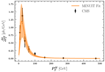
Figure 1: The combined measurement of differential cross section for $H\rightarrow\gamma\gamma$, $H\rightarrow ZZ^{*}$ and $H\rightarrow b\bar{b}$ decay channels as a function of $p_{\mathrm{T}}^{H}$ is shown as black points with error bars CMS:2018gwt . Using the MINUIT package James:1994vla , the spectra are fitted to the Tsallis function for $q=1.79\pm 0.13$ and $T_{0}=3.7\pm 0.8\,\mathrm{GeV}$.

IV Acknowledgments

The author would like to thank Amjad Ashoorioon and Abasalt Rostami for useful comments, and Hadi Hashamipour for the help to provide the figure.

References

- (1) G. Aad et al. [ATLAS], “Observation of a new particle in the search for the Standard Model Higgs boson with the ATLAS detector at the LHC,” Phys. Lett. B 716, 1-29 (2012) [arXiv:1207.7214 [hep-ex]].
- (2) S. Chatrchyan et al. [CMS], “Observation of a New Boson at a Mass of 125 GeV with the CMS Experiment at the LHC,” Phys. Lett. B 716, 30-61 (2012) [arXiv:1207.7235 [hep-ex]].
- (3) S. Chatrchyan et al. [CMS], “Observation of a New Boson with Mass Near 125 GeV in Collisions at = 7 and 8 TeV,” JHEP 06, 081 (2013) [arXiv:1303.4571 [hep-ex]].
- (4) M. J. G. Veltman, “The Infrared - Ultraviolet Connection,” Acta Phys. Polon. B 12, 437 (1981).
- (5) P. Draper and H. Rzehak, “A Review of Higgs Mass Calculations in Supersymmetric Models,” Phys. Rept. 619, 1-24 (2016) [arXiv:1601.01890 [hep-ph]].
- (6) G. Panico and A. Wulzer, “The Composite Nambu-Goldstone Higgs,” Lect. Notes Phys. 913, pp.1-316 (2016) [arXiv:1506.01961 [hep-ph]].
- (7) M. Ahmadvand, “Matter and dark matter asymmetry from a composite Higgs model,” Eur. Phys. J. C 81, no.4, 358 (2021) [arXiv:2010.10121 [hep-ph]].
- (8) B. B. Mandelbrot, “The Fractal Geometry of Nature,” W. H. Freeman and Company: New York, USA (1983).
- (9) R. Hagedorn, “Statistical thermodynamics of strong interactions at high-energies,” Nuovo Cim. Suppl. 3, 147-186 (1965) CERN-TH-520.
- (10) S. C. Frautschi, “Statistical bootstrap model of hadrons,” Phys. Rev. D 3, 2821-2834 (1971).
- (11) G. F. Chew, “Hadron bootstrap hypothesis,” Phys. Rev. D 4, 2330-2335 (1971).
- (12) I. Bediaga, E. M. F. Curado and J. M. de Miranda, “A Nonextensive thermodynamical equilibrium approach in e+ e- — hadrons,” Physica A 286, 156-163 (2000) [arXiv:hep-ph/9905255 [hep-ph]].
- (13) J. Cleymans and D. Worku, “The Tsallis Distribution in Proton-Proton Collisions at = 0.9 TeV at the LHC,” J. Phys. G 39, 025006 (2012) [arXiv:1110.5526 [hep-ph]].
- (14) L. Marques, E. Andrade-II and A. Deppman, “Nonextensivity of hadronic systems,” Phys. Rev. D 87, no.11, 114022 (2013) [arXiv:1210.1725 [hep-ph]].
- (15) A. Deppman, E. Megias and D. P. Menezes, “Fractals, nonextensive statistics, and QCD,” Phys. Rev. D 101, no.3, 034019 (2020) [arXiv:1908.08799 [hep-th]].
- (16) C. Tsallis, “Possible Generalization of Boltzmann-Gibbs Statistics,” J. Statist. Phys. 52, 479-487 (1988).
- (17) E. M. F. Curado and C. Tsallis, “Generalized statistical mechanics: Connection with thermodynamics,” J. Phys. A 24, L69-L72 (1991) [erratum: J. Phys. A 25, 1019 (1992)] CBPF-NF-041-90.
- (18) H. Lehmann, K. Symanzik and W. Zimmermann, “On the formulation of quantized field theories,” Nuovo Cim. 1, 205-225 (1955).
- (19) B. I. Abelev et al. [STAR], “Strange particle production in p+p collisions at s**(1/2) = 200-GeV,” Phys. Rev. C 75, 064901 (2007) [arXiv:nucl-ex/0607033 [nucl-ex]].
- (20) G. Aad et al. [ATLAS], “Charged-particle multiplicities in pp interactions measured with the ATLAS detector at the LHC,” New J. Phys. 13, 053033 (2011) [arXiv:1012.5104 [hep-ex]].
- (21) A. Adare et al. [PHENIX], “Identified charged hadron production in collisions at and 62.4 GeV,” Phys. Rev. C 83, 064903 (2011) [arXiv:1102.0753 [nucl-ex]].
- (22) K. Aamodt et al. [ALICE], “Production of pions, kaons and protons in collisions at GeV with ALICE at the LHC,” Eur. Phys. J. C 71, 1655 (2011) [arXiv:1101.4110 [hep-ex]].
- (23) V. Khachatryan et al. [CMS], “Strange Particle Production in Collisions at and 7 TeV,” JHEP 05, 064 (2011) [arXiv:1102.4282 [hep-ex]].
- (24) A. M. Sirunyan et al. [CMS], “Measurement and interpretation of differential cross sections for Higgs boson production at 13 TeV,” Phys. Lett. B 792, 369-396 (2019) [arXiv:1812.06504 [hep-ex]].
- (25) M. Aaboud et al. [ATLAS], “Combined measurement of differential and total cross sections in the and the decay channels at TeV with the ATLAS detector,” Phys. Lett. B 786, 114-133 (2018) [arXiv:1805.10197 [hep-ex]].
- (26) F. James, “MINUIT Function Minimization and Error Analysis: Reference Manual Version 94.1,” CERN-D-506.
- (27) L. Reina, “TASI 2011: lectures on Higgs-Boson Physics,” [arXiv:1208.5504 [hep-ph]].