Generalized Langevin equation with fluctuating diffusivity

Abstract

A generalized Langevin equation with fluctuating diffusivity (GLEFD) is proposed, and it is shown that the GLEFD satisfies a generalized fluctuation-dissipation relation. If the memory kernel is a power law, the GLEFD exhibits subdiffusion, non-Gaussianity, and stretched-exponential relaxation. The case in which the memory kernel is given by a single exponential function is also investigated as an analytically tractable example. In particular, the mean-square displacement and the self-intermediate-scattering function of this system show plateau structures. A numerical scheme to integrate the GLEFD is also presented.

I Introduction

A microscopic tagged-particle suspended in a fluid exhibits random motion called Brownian motion, which is caused by incessant collisions with solvent molecules of the fluid Dhont (1996). In a dilute and homogeneous condition, the particle shows normal diffusion, which is characterized by a linear increase of the mean-square displacement (MSD) with a constant diffusion coefficient. However, the tagged-particle diffusion in crowded and/or heterogeneous environments (e.g., cytoplasm of living cells) shows intrinsic statistical properties such as anomalous diffusion, non-Gaussianity, and random diffusivity He et al. (2008); Wang et al. (2012); Parry et al. (2014); Manzo et al. (2015); Lampo et al. (2017); Sabri et al. (2020); Janczura et al. (2021). Because cell functions depend on intracellular transport of macromolecules, elucidation of these statistical properties is crucially important to understand complex mechanisms of living cells Berg et al. (1981); Bressloff and Newby (2013).

Anomalous diffusion is characterized by a non-linear increase of the MSD; in particular, if the MSD increases sublinearly, it is referred to as subdiffusion. There are several possible mechanisms for such non-linear behavior. One of the important mechanisms of subdiffusion is a memory effect or viscoelastic properties of a surrounding medium Goychuk (2009, 2012); Goychuk and Pöschel (2021). The memory effect originates from interactions with surrounding molecules, and analytically obtained by a projection operator method from microscopic equations of motion Kubo et al. (1991); Götze (2009); Hansen and McDonald (1990). Dynamics of a tagged particle with the memory effect is described by the generalized Langevin equation (GLE); the memory effect is represented by an integral term with a memory kernel. If the memory kernel is a power-law form, the MSD shows subdiffusion, whereas the displacement is always Gaussian, because the GLE is a Gaussian process (if there is no external force).

In contrast, the random diffusivity is usually generated either by dynamics of internal modes of the tagged particle or by heterogeneity of the medium. For example, center-of-mass motions of several polymer models show the fluctuating diffusivity due to dynamics of internal modes Uneyama et al. (2015); Miyaguchi (2017); Nampoothiri et al. (2021); Yamamoto et al. (2021); Nampoothiri et al. (2022). As an example of the heterogeneity, diffusion on random potentials also gives rise to the random diffusivity Miyaguchi and Akimoto (2011, 2015). One of important consequences of the random diffusivity is the non-Gaussianity of the particle displacement. However, the MSD for the random diffusivity models shows only normal diffusion, if the system is in equilibrium Miyaguchi et al. (2016); Jain and Sebastian (2016); Chechkin et al. (2017); Tyagi and Cherayil (2017); Lanoiselée and Grebenkov (2018).

Single-particle-tracking experiments He et al. (2008); Parry et al. (2014); Manzo et al. (2015); Sabri et al. (2020); Janczura et al. (2021) and molecular dynamics simulations Akimoto et al. (2011); Yamamoto et al. (2014); Jeon et al. (2016); Yamamoto et al. (2017) show that tagged particles exhibit subdiffusion, fluctuating diffusivity, and non-Gaussianity. Thus it is important to incorporate the fluctuating diffusivity into diffusion processes with a memory effect such as the GLE. In fact, to describe the diffusion process observed in complex media such as the cytoplasm, phenomenological models which combine these two effects have recently been proposed and studied Chechkin et al. (2017); Ślęzak et al. (2018); Wang et al. (2020a, b); Sabri et al. (2020); Janczura et al. (2021); Dieball et al. (2022); Goswami and Chakrabarti (2022). However, physical backgrounds of these phenomenological models have been still unclear. For example, the fluctuation-dissipation relation and the detailed balance should be satisfied if the system is in equilibrium Kou (2008), but it has not been elucidated so far whether these properties hold for the phenomenological models.

This article proposes and investigates a GLE with fluctuating diffusivity (GLEFD). By using a Markovian embedding method Goychuk (2009, 2012), the fluctuating diffusivity is incorporated into an overdamped GLE. Importantly, it is shown that the GLEFD satisfies a generalized fluctuation-dissipation relation. Moreover, a numerical scheme for the GLEFD is also presented on the basis of the Markovian embedding.

Then, as an important example, the GLEFD with a power-law memory kernel is investigated, and show that this system exhibits both subdiffusion and non-Gaussianity. In addition, as one of the simplest models, we study the GLEFD with an exponential memory kernel, which is referred to as a dimer model. Due to its simplicity, this dimer model can be analytically tractable to some extent. In fact, analytical formulas for the MSD, a non-Gaussian parameter (NGP), and a self-intermediate-scattering function (ISF) are derived. Furthermore, as a special class of the dimer model, we also study the case in which the diffusion coefficient switches between two values, $D_{+}$ and $D_{-}$, alternately, and the distributions of the sojourn times in these two states are given by an exponential distribution or a power law. In these special classes of the GLEFD, it is assumed that a short-time diffusivity is not fluctuating, and thus only a long-time diffusivity is fluctuating.

This paper is organized as follows. In Sec. II, the GLE and the Markovian embedding are briefly summarized; then, we incorporate the fluctuating diffusivity into the GLE, and thereby defining the GLEFD. The numerical scheme of the GLEFD is also presented in this section. In Sec. III, the case in which the memory kernel is a power-law form is studied. Moreover, Secs.IV and V are devoted to investigation of the dimer model, of which the memory kernel is a single exponential function. Finally, in Sec. VI, a discussion on the significance and implication of the results is presented. Some technical matters including numerical setups are presented in Appendices.

II Generalized Langevin equation with fluctuating diffusivity

The Langevin equation with fluctuating diffusivity has been studied intensively during the last decade Chubynsky and Slater (2014); Uneyama et al. (2015); Miyaguchi (2017), and its properties are now very well known. The memory kernel of this model is given by a delta function and thus there is no integral term in this equation, whereas a difficulty in introducing the fluctuating diffusivity into the GLE is in the presence of an integral term. This motivates us to transform the GLE into a form without the integral term by the Markovian embedding method, and then to introduce the fluctuating diffusivity into this Markovian system.

II.1 Generalized Langevin equation

First, let us briefly introduce an overdamped GLE (without fluctuating diffusivity) of the following form:

$$\zeta\frac{d\bm{r}(t)}{dt}+\zeta\int_{0}^{t}\phi(t-t^{\prime})\dot{\bm{r}}(t^{\prime})dt^{\prime}={\color[rgb]{0,0,0}\bm{F}_{e}}+\bm{\xi}(t)+{\color[rgb]{0,0,0}\bm{\xi}_{c}^{0}(t)},$$ (1)

where the tagged-particle position $\bm{r}(t)$ and an external force $\bm{F}_{e}(\bm{r},t)=-\partial V(\bm{r},t)/\partial\bm{r}$ are $n$ dimensional vectors , and the overdot in $\dot{\bm{r}}$ denotes the time derivative. Moreover, $\bm{\xi}(t)$ and $\bm{\xi}_{c}^{0}(t)$ in Eq. (1) are $n$-dimensional Gaussian noises, and if the system is in equilibrium, they should satisfy the fluctuation-dissipation relations:

$$\left\langle\bm{\xi}(t)\bm{\xi}(t^{\prime})\right\rangle =2k_{B}T\zeta\delta(t-t^{\prime})\bm{I},$$ (2)

$$\left\langle\bm{\xi}_{c}^{0}(t)\bm{\xi}_{c}^{0}(t^{\prime})\right\rangle =k_{B}T\zeta\phi(t-t^{\prime})\bm{I}.$$ (3)

Here $k_{B}$ is the Boltzmann constant, $T$ is the absolute temperature, and $\bm{I}$ is the $n\times n$ identity tensor. Moreover, $\delta(t)$ is the delta function, and $\phi(t)$ is the memory kernel, which is an even function of $t$. Accordingly, $\bm{\xi}(t)$ is a white noise, and $\bm{\xi}_{c}^{0}(t)$ a correlated noise; the superscript $0$ in $\bm{\xi}_{c}^{0}(t)$ indicates the absence of the fluctuating diffusivity. $\zeta$ is the friction constant with respect to the white noise, but $\zeta$ is also put in front of the integral term in Eq. (1) just to make $\phi(t)dt$ dimensionless.

In some literature, the model without the friction term $\zeta\dot{\bm{r}}(t)$ or the white Gaussian noise $\bm{\xi}(t)$ in Eq. (1) is studied Deng and Barkai (2009); Jeon and Metzler (2012); Kou (2008). For the monomer dynamics of the Rouse model, however, it is shown that these terms naturally arise Panja (2010). In addition, if the friction term $\zeta\dot{\bm{r}}(t)$ and the white Gaussian noise $\bm{\xi}(t)$ in Eq. (1) are absent, the integral equation (1) does not have a solution $\bm{v}(t)=\dot{\bm{r}}(t)$ in general Doetsch (2012). Thus, the incorporation of these terms might well be physically natural. In addition, the friction term $\zeta\dot{\bm{r}}(t)$ plays an essential role in constructing Markovian equations of motion below.

For simplicity, we rewrite Eq. (1) as

$$\frac{d\bm{r}}{dt}+\int_{0}^{t}\phi(t-t^{\prime})\dot{\bm{r}}(t^{\prime})dt^{\prime}=\beta D\bm{F}_{e}+\sqrt{2D}\bm{\xi}+\sqrt{D}\bm{\xi}_{c}^{0},$$ (4)

where $D:=k_{B}T/\zeta$ is the diffusion coefficient with respect to the white Gaussian noise $\bm{\xi}(t)$, and $\beta=1/k_{B}T$ is the inverse temperature. In Eq. (4), $\bm{\xi}(t)$ and $\bm{\xi}_{c}^{0}(t)$ are redefined as $\bm{\xi}\to\bm{\xi}(2k_{B}T\zeta)^{1/2}$ and $\bm{\xi}_{c}^{0}\to\bm{\xi}_{c}^{0}(k_{B}T\zeta)^{1/2}$ instead of defining new variables. Accordingly, the fluctuation-dissipation relations [Eqs. (2) and (3)] are modified as

$$\left\langle\bm{\xi}(t)\bm{\xi}(t^{\prime})\right\rangle =\delta(t-t^{\prime})\bm{I},$$ (5)

$$\left\langle\bm{\xi}_{c}^{0}(t)\bm{\xi}_{c}^{0}(t^{\prime})\right\rangle =\phi(t-t^{\prime})\bm{I}.$$ (6)

II.2 Markovian embedding

To incorporate fluctuating diffusivity into Eq. (4), we use the Markovian embedding method Goychuk (2009). First, the correlated noise $\bm{\xi}_{c}^{0}(t)$ is approximated as a superposition of stochastic processes $\bm{\xi}_{i}(t)$ as

$$\bm{\xi}_{c}^{0}(t)\approx\sum_{i=0}^{N-1}\bm{\xi}_{i}(t),$$ (7)

where $\bm{\xi}_{i}(t)$ is assumed to satisfy the equation for the Ornstein-Uhlenbeck process:

$$\frac{d\bm{\xi}_{i}(t)}{dt}=-\nu_{i}\bm{\xi}_{i}(t)+\sqrt{2k_{i}^{\prime}\nu_{i}}\bm{\eta}_{i}(t).$$ (8)

Here, $\nu_{i}$ and $k_{i}^{\prime}$ are positive constants to be specified below [Eq. (11)], and $\bm{\eta}_{i}(t)$ is a white Gaussian noise with

$$\left\langle\bm{\eta}_{i}(t)\bm{\eta}_{j}(t^{\prime})\right\rangle=\delta_{ij}\delta(t-t^{\prime})\bm{I}.$$ (9)

We also assume that $\bm{\eta}_{i}(t)$ and $\bm{\xi}(t)$ are independent, and that $\bm{\xi}_{i}(t)$ is in equilibrium, and thus $\bm{\xi}_{i}(t)$ follows a canonical distribution $\propto\exp(-\bm{\xi}_{i}^{2}/2k^{\prime}_{i})$; the latter assumption is necessary to make $\bm{\xi}_{c}^{0}(t)$ a stationary process [Eq. (6)].

Then, from Eqs. (8) and (9), a correlation matrix for $\bm{\xi}_{i}(t)$ is given by

$$\left\langle\bm{\xi}_{i}(t)\bm{\xi}_{j}(t^{\prime})\right\rangle=k_{i}^{\prime}\delta_{ij}e^{-\nu_{i}|t-t^{\prime}|}\bm{I}.$$ (10)

From Eqs. (6), (7), and (10), we have an approximation to the correlation function $\phi(t)$ as

$$\phi(t)\approx\sum_{i=0}^{N-1}k_{i}^{\prime}e^{-\nu_{i}|t|}.$$ (11)

The parameters $k_{i}^{\prime}$ and $\nu_{i}$ are determined so that Eq. (11) holds approximately. Thus, the above equation is an approximation to $\phi(t)$ with a superposition of exponential functions, but if $N$ tends to infinity, the approximation is expected to become exact Goychuk (2009).

Next, to deal with the integral term in Eq. (4), let us define auxiliary variables $\bm{r}_{i}(t)$ as Goychuk (2012)

$$k_{i}^{\prime}(\bm{r}_{i}-\bm{r})=\sqrt{D}\bm{\xi}_{i}-k_{i}^{\prime}\int_{0}^{t}e^{-\nu_{i}(t-t^{\prime})}\dot{\bm{r}}(t^{\prime})dt^{\prime},$$ (12)

Inserting Eqs. (7) and (11) into Eq. (4), we have the Markovian equations of motion as

$$\frac{d\bm{r}(t)}{dt} =\beta D\bm{F}_{e}+\sqrt{2D}\bm{\xi}(t)-\beta D\sum_{i=0}^{N-1}k_{i}(\bm{r}-\bm{r}_{i}),$$ (13)

$$\frac{d\bm{r}_{i}(t)}{dt} =-\beta D_{i}k_{i}(\bm{r}_{i}-\bm{r})+\sqrt{2D_{i}}\bm{\eta}_{i}(t),$$ (14)

where the second equation is obtained by differentiating Eq. (12) with time $t$. Here, $k_{i}:=k_{i}^{\prime}/\beta D$ corresponds to a spring constant, and $D_{i}:=\nu_{i}/k_{i}\beta$ is a diffusivity of the auxiliary variable $\bm{r}_{i}$. In this way, the GLE [Eq. (1)] is transformed into a Markovian system [Eqs. (13) and (14)], in which the tagged particle $\bm{r}$ interacts with the auxiliary variables $\bm{r}_{i}$ through harmonic potentials. In addition, Eqs. (5) and (9) are the fluctuation-dissipation relations for Eqs. (13) and (14). If the friction term $d\bm{r}(t)/dt$ is absent in Eq. (4), then Eq. (13) becomes an algebraic equation.

The Markovian embedding of the underdamped GLE is presented in Ref. Goychuk (2009), whereas Eqs. (13) and (14) are a Markovian embedding for the overdamped GLE. Obviously, Eqs. (13) and (14) can be readily utilized as a numerical scheme to simulate the non-Markovian equation (4). It is also the case even if we introduce the fluctuating diffusivity into Eq. (14) as shown below.

In this work, any physical meanings of the auxiliary variables are not considered explicitly, but they should be related to fast variables which are projected out from microscopic equations of motion. This is because the GLE is usually obtained by projecting out fast variables, and $\phi(t)$ and $\bm{\xi}_{c}^{0}(t)$ in the GLE [Eq. (4)] are related to these fast variables Hansen and McDonald (1990). As an example, it is known that the middle monomer of the Rouse polymer chain can be described by Eqs. (13) and (14) with suitable choices of $D_{i}$ and $k_{i}$ Panja (2010). In this example, the auxiliary variables are normal modes of the Rouse polymer, and the kernel $\phi(t)$ is a power-law function with an exponential cutoff.

II.3 Fluctuating diffusivity

Now, we incorporate the fluctuating diffusivity into Eq. (14) as

$$\frac{d\bm{r}_{i}(t)}{dt}=-\beta k_{i}D_{i}(t)(\bm{r}_{i}-\bm{r})+\sqrt{2D_{i}(t)}\bm{\eta}_{i}(t),$$ (15)

where the fluctuating diffusivity $D_{i}(t)$ is a stochastic process. We assume that $D_{i}(t)$ and $\bm{\eta}_{j}(t)$ are independent for any $i$ and $j$. In contrast, Eq. (13) remains unchanged. Note that the fluctuation-dissipation relation and the detailed balance hold for Eqs. (13) and (15), and thus, if $D_{i}(t)$ are stationary processes as well, the whole process is in equilibrium.

Next, let us derive an integro-differential equation similar to Eq. (4). According to the modification from Eq. (14) to Eq. (15), Eqs. (8) and (10) are also modified respectively as

$$\frac{d\bm{\xi}_{i}(t)}{dt} =-\nu_{i}(t)\bm{\xi}_{i}(t)+\sqrt{2k_{i}^{\prime}\nu_{i}(t)}\bm{\eta}_{i}(t),$$ (16)

$$\left\langle\bm{\xi}_{i}(t)\bm{\xi}_{j}(t^{\prime})\right\rangle =k_{i}^{\prime}\delta_{ij}\bm{I}e^{-\left|\int_{t^{\prime}}^{t}\nu_{i}(u)du\right|},$$ (17)

where $\nu_{i}(t):=\beta k_{i}D_{i}(t)$ and $\bm{\eta}_{i}(t)$ is the white Gaussian noise satisfying Eq. (9). Thus, $\nu_{i}(t)$ is the inverse of an fluctuating relaxation time, but, for simplicity, $\nu_{i}(t)$ is also referred to as the fluctuating diffusivity.

From Eqs. (15) and (16), we obtain

$$k_{i}^{\prime}\frac{d}{dt}\left(\bm{r}_{i}-\bm{r}\right)=-k_{i}^{\prime}\dot{\bm{r}}-k_{i}^{\prime}\nu_{i}(t)(\bm{r}_{i}-\bm{r})+\sqrt{D}\left[\dot{\bm{\xi}}_{i}+\nu_{i}(t)\bm{\xi}_{i}\right].$$ (18)

A solution of this equation is given by

$$k_{i}^{\prime}\left(\bm{r}_{i}-\bm{r}\right)=\sqrt{D}{\bm{\xi}}_{i}-k_{i}^{\prime}\int_{0}^{t}e^{-\int_{t^{\prime}}^{t}\nu_{i}(u)du}\dot{\bm{r}}(t^{\prime})dt^{\prime},$$ (19)

as can be checked directly by differentiating Eq. (19) in terms of $t$. Inserting Eq. (19) into Eq. (13), we finally obtain the GLEFD

$$\frac{d\bm{r}}{dt}+\int_{0}^{t}\phi(t,t^{\prime})\dot{\bm{r}}(t^{\prime})dt^{\prime}=\beta D\bm{F}_{e}+\sqrt{2D}\bm{\xi}+\sqrt{D}\bm{\xi}_{c},$$ (20)

with a generalized fluctuation-dissipation relation

$$\left\langle\bm{\xi}_{c}(t)\bm{\xi}_{c}(t^{\prime})\right\rangle=\phi(t,t^{\prime})\bm{I}:=\bm{I}\sum_{i=0}^{N-1}k_{i}^{\prime}e^{-\left|\int_{t^{\prime}}^{t}\nu_{i}(u)du\right|}.$$ (21)

The memory kernel $\phi(t,t^{\prime})$, which is defined by the second equality in Eq. (21), depends on the fluctuating diffusivity $\nu_{i}(u)$. In other words, $\phi(t,t^{\prime})$ is a functional of $\nu_{i}(t)$. As in the case of $\bm{\xi}_{c}^{0}(t)$ [Eq. (7)], $\bm{\xi}_{c}(t)$ in Eq. (20) is given by

$$\bm{\xi}_{c}(t)=\sum_{i=0}^{N-1}\bm{\xi}_{i}(t),$$ (22)

where $\bm{\xi}_{i}(t)$ is redefined by Eqs. (16) and (17). Therefore, the diffusivity due to $\bm{\xi}_{c}(t)$ is fluctuating; the absence of the superscript $0$ in $\bm{\xi}_{c}(t)$ indicates the presence of the fluctuating diffusivity. Moreover, Eqs. (13) and (15) can be utilized as a numerical scheme for the GLEFD [Eq. (20)],

In Eq. (21), it looks as if time-translation invariance is violated, but it is not the case. This apparent violation is due to the fact that Eq. (21) is a formula for a single realization of diffusivity paths [$\nu_{i}(t)$]. If the diffusivities $\nu_{i}(t)$ are stationary processes and initially in equilibrium, then, by taking ensemble averages over the diffusivity paths and the initial conditions in Eq. (21), we have a fluctuation-dissipation relation with the time-translation invariance as

$$\left\langle\left\langle\bm{\xi}_{c}(t)\bm{\xi}_{c}(t^{\prime})\right\rangle\right\rangle_{\nu}=\phi_{\nu}(t-t^{\prime})\bm{I}:=\bm{I}\sum_{i=0}^{N-1}k_{i}^{\prime}\left\langle e^{-\left|\int_{t^{\prime}}^{t}\nu_{i}(u)du\right|}\right\rangle_{\nu},$$ (23)

where $\phi_{\nu}(t-t^{\prime})$ is defined by the right-hand side of the above equation.

Note also that the diffusivity $D$ with respect to the white noise $\bm{\xi}(t)$ remains constant in Eq. (20), because a goal of this work was to incorporate the fluctuating diffusivity into the correlated noise $\bm{\xi}_{c}^{0}(t)$ in Eq. (4). Moreover, the correlated noise $\bm{\xi}_{c}(t)$ in Eq. (20) is defined through the Ornstein-Uhlenbeck processes $\bm{\xi}_{i}(t)$ with fluctuating diffusivity [Eq. (16)], but the variance of $\bm{\xi}_{i}(t)$ and hence also the variance of $\bm{\xi}_{c}(t)$ are independent of time due to the detailed balance. Thus, only their relaxation behavior is fluctuating, but, as shown in the next section, the long-time (generalized) diffusivity of $\bm{r}(t)$ is fluctuating; this is why we refer to the model defined by Eq. (20) as the GLEFD.

Due to coexistence of trajectories with different diffusivity paths $D_{i}(u)$, the position vectors $\bm{r}_{i}(t)$ and $\bm{r}(t)$ are non-Gaussian processes Uneyama et al. (2019). For fixed paths $D_{i}(u)$ [or, equivalently, fixed $\nu_{i}(u)$], however, $\bm{r}_{i}(t)$ and $\bm{r}(t)$ are Gaussian processes (if the external force $\bm{F}_{e}$ is absent). This is because Eqs. (13) and (15) are linear in $\bm{r}_{i}(t)$ and $\bm{r}(t)$. Thanks to this pathwise Gaussianity, the ISF for the dimer model can be easily derived as shown in Sec. IV. If we take into account more than one realization of the diffusivity paths $[D_{i}(u)]$, $\bm{r}_{i}(t)$ and $\bm{r}(t)$ become non-Gaussian processes.

In Ref. Ślęzak et al. (2018), the GLE with a random parameter is proposed, but the random parameter is assumed to be time independent. Namely, the model in Ref. Ślęzak et al. (2018) is a compound GLE, in which GLEs with different parameter values are simply superimposed. In Eq. (20), however, the random diffusivity $\nu_{i}(t)$ is time dependent and fluctuating, and this makes the theoretical analysis of Eq. (20) quite difficult. In fact, the integral term in Eq. (20) is not a convolution, and thus it is impossible to use the Laplace transformation, which is a standard method to analyze the GLE Pottier (2003); Burov and Barkai (2008).

III Fractional Brownian motion with fluctuating diffusivity

In this section, we study the GLEFD with a power-law memory kernel, which might well be important to explain subdiffusion and non-Gaussianity observed in biological experiments Sabri et al. (2020); Janczura et al. (2021). Numerical simulations show that the GLEFD with a power-law memory kernel exhibits subdiffusion, non-Gaussianity, and stretched-exponential relaxation.

III.1 Fractional Brownian motion

First, let us study the GLE [Eq. (4)] without the fluctuating diffusivity or the external force $\bm{F}_{e}$:

$$\frac{d\bm{r}}{dt}+\int_{0}^{t}\phi(t-t^{\prime})\dot{\bm{r}}(t^{\prime})dt^{\prime}=\sqrt{2D}\bm{\xi}+\sqrt{D}\bm{\xi}_{c}^{0}.$$ (24)

Here, the memory kernel $\phi(t-t^{\prime})$ is assumed to be given by a power law

$$\phi(t)=\frac{D}{D_{\alpha}}\frac{t^{-\alpha}}{\Gamma(1+\alpha)\Gamma(1-\alpha)}=At^{-\alpha},$$ (25)

where $\alpha$ is the power-law index with $0<\alpha<1$, $\Gamma(\dots)$ is the Gamma function, $D_{\alpha}$ is a generalized diffusion coefficient of subdiffusion, and $A:=D/D_{\alpha}\Gamma(1+\alpha)\Gamma(1-\alpha)$.

It is often important to take into account cutoffs of the power-law kernel in studying real phenomena Pottier (2003); Panja (2010); Molina-Garcia et al. (2018). In addition, in approximating the power-law kernel with Eq. (11), short- and long-time cutoffs are unavoidable as explained shortly. Therefore, the numerical scheme proposed in the previous section entails errors caused by these cutoffs at short and long times [but, the short-time cutoff might not matter due to the presence of the white noise $\bm{\xi}(t)$ in Eq. (4)]. Here, however, we focus only on pure power-law time regimes, in which cutoff effects are negligible Goychuk (2009).

With the memory kernel defined in Eq. (25), the GLE without the fluctuating diffusivity [Eq. (24)] shows normal diffusion at short time and subdiffusion at long time as Panja (2010); Pottier (2003) (See also Appendix A)

$$\left\langle\delta\bm{r}^{2}(t)\right\rangle\simeq\begin{cases}2nDt&t\ll t_{c},\\ 2nD_{\alpha}t^{\alpha}&t\gg t_{c},\end{cases}$$ (26)

where $\delta\bm{r}(t)$ is a displacement vector defined as $\delta\bm{r}(t):=\bm{r}(t)-\bm{r}(0)$, and a crossover time $t_{c}$ is $t_{c}:=[\Gamma(1+\alpha)D_{\alpha}/D]^{1/(1-\alpha)}$. More precisely, the displacement correlation $\left\langle\bm{r}(t)\bm{r}(t^{\prime})\right\rangle$ is given by $\left\langle\bm{r}(t)\bm{r}(t^{\prime})\right\rangle\simeq D_{\alpha}(t^{\alpha}+t^{\prime\alpha}-|t-t^{\prime}|^{\alpha})$ at long times, and thus hereafter this model is referred to as the fractional Brownian motion (FBM), although short-time behavior is different from the original FBM Kou (2008).

To obtain the Markovian embedding of Eq. (24), let us put $k_{i}^{\prime}=A^{\prime}\nu_{i}^{\alpha}$ with $A^{\prime}:=A(b-1)/b^{1/2}\Gamma(\alpha)$ in Eq. (11), and then the power-law kernel [Eq. (25)] is approximated as

$$\phi(t)\approx A^{\prime}\sum_{i=0}^{N-1}\nu_{i}^{\alpha}e^{-\nu_{i}|t|},$$ (27)

where $\nu_{i}:=\nu_{0}/b^{i}$ with a constant $b>1$ and a high frequency cutoff $\nu_{0}$ Goychuk (2009). Then, Eq. (27) can be approximated by an integral as $\approx A^{\prime}\int_{0}^{\infty}\nu^{\alpha-1}e^{-\nu t}d\nu b^{1/2}/(b-1)=A^{\prime}t^{-\alpha}\Gamma(\alpha)b^{1/2}/(b-1)=At^{-\alpha}$, and therefore we obtain Eq. (25). This integral approximation is exact at $b\to 1$ and $N\to\infty$, but, it is found that the choices $b=2$, $N=128$, and $\nu_{0}=1000/\mu_{+}$ are sufficiently good to describe Eq. (25) in numerical simulations for the two-state model defined below [Eq. (30)]. See Appendix D for simulation detail.

III.2 Fluctuating diffusivity: two-state model

Here, we derive and analyze the GLEFD [Eq. (20)] with a power-law memory kernel; this model is referred to as FBM with fluctuating diffusivity (FBMFD). The equation of motion is given by Eq. (20) without the external force $\bm{F}_{e}$

$$\frac{d\bm{r}}{dt}+\int_{0}^{t}\phi(t,t^{\prime})\dot{\bm{r}}(t^{\prime})dt^{\prime}=\sqrt{2D}\bm{\xi}(t)+\sqrt{D}\bm{\xi}_{c}(t).$$ (28)

Because of the correspondence between Eq. (11) and Eq. (21), the memory kernel $\phi(t,t^{\prime})$ is obtained by modifying Eq. (27) as

$$\phi(t,t^{\prime}):=A^{\prime}\sum_{i=0}^{N-1}\nu_{i}^{\alpha}e^{-\left|\int_{t^{\prime}}^{t}\nu_{i}(u)du\right|}.$$ (29)

As a simple case study, let us focus on the FBMFD with a two-state diffusivity. The two-state diffusivity has been used frequently to explain statistical properties of single-particle-tracking data Sabri et al. (2020); Janczura et al. (2021); Dieball et al. (2022). The two-state diffusivity is defined by

$$\nu_{i}(t)=\nu_{i}\kappa(t)=\begin{cases}\nu_{i}\kappa_{+},\\[2.84544pt] \nu_{i}\kappa_{-},\end{cases}$$ (30)

where $\nu_{i}(t)=\beta k_{i}D_{i}(t)$ as before, $\nu_{i}$ are constants with the same dimension as $\nu_{i}(t)$, and $\kappa(t)$ is a dimensionless two-state process Godrèche and Luck (2001); Miyaguchi et al. (2019, 2016).

More precisely, the diffusivity $\nu_{i}(t)$ is assumed to switch between the two states at random times $t_{1},t_{2},\dots$. Let $\tau_{k}:=t_{k}-t_{k-1}\,(k=1,2,\dots)$ be sojourn times of the two states, where we define $t_{0}=0$ for convenience. The $+$ ($-$) state is referred to as the fast (slow) state, and the sojourn time distribution of the fast (slow) state is denoted as $\rho^{+}(\tau)$ [$\rho^{-}(\tau)$]. In the numerical simulations of the FBMFD, $\rho^{\pm}(\tau)$ are assumed to follow exponential distributions with means $\mu_{\pm}$ [Eq. (115)].

By using Eq. (30), Eq. (21) is rewritten as

$$\phi(t,t^{\prime}):=A^{\prime}\sum_{i=0}^{N-1}\nu_{i}^{\alpha}e^{-\nu_{i}\left|\int_{t^{\prime}}^{t}\kappa(u)du\right|},$$ (31)

where $k_{i}^{\prime}$ is set as $k_{i}^{\prime}=A^{\prime}\nu_{i}^{\alpha}$ as in the case of the FBM. If there is no switching, the diffusive state is $\nu_{i}(t)\equiv\nu_{i}\kappa_{+}$ or $\nu_{i}(t)\equiv\nu_{i}\kappa_{-}$ for all $t$ depending on the initial state. It follows that, if the initial state is $\pm$, the MSD grows as $\left\langle\delta\bm{r}^{2}(t)\right\rangle\simeq 2nD_{\alpha}^{\pm}t^{\alpha}$ with $D^{\pm}_{\alpha}=D_{\alpha}\kappa_{\pm}^{\alpha}$ at long time. If the diffusive state switches very slowly between the two states, the diffusivity might be regarded as being fluctuating between the two diffusion coefficients $D_{\alpha}^{\pm}$.

It is not that simple in general, however, because, if the diffusive state switches from one state to the other, information of the previous state is not lost immediately due to the memory effect represented by the integral in Eq. (31). In fact, by setting $\nu_{i}=\nu_{0}/b^{i}$ and using the integral approximation mentioned above, Eq. (31) can be expressed as

$$\phi(t,t^{\prime})\approx\frac{D}{D_{\alpha}}\frac{\left|\int_{t^{\prime}}^{t}\kappa(u)du\right|^{-\alpha}}{\Gamma(1+\alpha)\Gamma(1-\alpha)}.$$ (32)

Note that, if $\kappa(t)$ is independent of time $t$, Eq. (32) represents an algebraic decay $\sim|t-t^{\prime}|^{-\alpha}$, thus it is a generalization of Eq. (25).

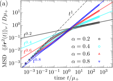
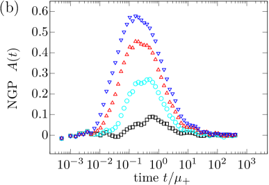
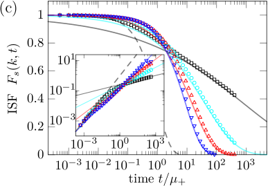
Figure 1: FBMFD for four different values of $\alpha$: $\alpha=0.2$, $0.4$, $0.6$, and $0.8$. The symbols are data obtained by numerical integration of Eqs. (13) and (15) with the correlation function in Eq. (31). The generalized diffusivity $D_{\alpha}$ is fixed as $D_{\alpha}/D\mu_{+}^{1-\alpha}=0.3$, the fast and slow state diffusivities $\kappa_{\pm}$ as $(\kappa_{+},\kappa_{-})=(1.0,0.01)$, and the mean sojourn time $\mu_{-}$ as $\mu_{-}=\mu_{+}$. (a) MSD vs time. The dashed line and the full lines are the short-time and long-time predictions in Eq. (34). (b) NGP vs time. (c) ISF vs time. The dashed line and the full lines are the short-time and long-time predictions in Eq. (35). The wave number $k$ is set as $k=1/\sqrt{D\mu_{+}}$. (inset) $\log[F_{s}(k,t)]$ vs $t$ in log-log form. [In (b-c), results for the four different values of $\alpha$ are displayed with the same color code as in (a)].

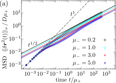
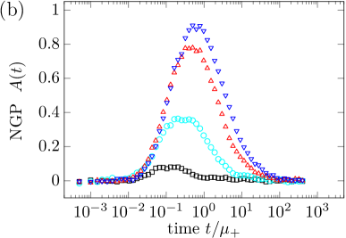
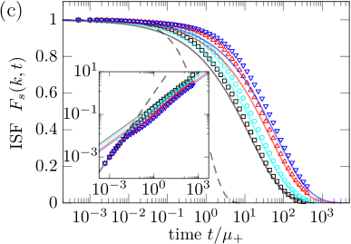
Figure 2: FBMFD for four different values of $\mu_{-}$: $\mu_{-}/\mu_{+}=0.2$, $1.0$, $3.0$, and $5.0$. The power-law index $\alpha$ is fixed as $\alpha=0.5$. Parameters $D_{\alpha}$, $\kappa_{\pm}$ and $k$ are the same as those in Fig. 1. (a) MSD vs time. The dashed line and the full lines are the short-time and long-time predictions in Eq. (34). (b) NGP vs time. (c) ISF vs time. The dashed line and the full lines are the short-time and long-time predictions in Eq. (35). (inset) $\log[F_{s}(k,t)]$ vs $t$ in log-log form. [In (b-c), results for the four different values of $\mu_{-}$ are displayed with the same color code as in (a)].

If $t-t^{\prime}$ is much larger than the mean sojourn times $\mu_{\pm}$, and $\kappa(t)$ is a stationary process with mean $\left\langle\kappa\right\rangle$, the integral in Eq. (32) can be approximated as $\int_{t^{\prime}}^{t}\kappa(s)ds\approx\left\langle\kappa\right\rangle(t-t^{\prime})$. Thus, for large $t-t^{\prime}$, we obtain

$$\phi(t,t^{\prime})\approx\frac{D}{D_{\alpha}^{\mathrm{eq}}}\frac{|t-t^{\prime}|^{-\alpha}}{\Gamma(1+\alpha)\Gamma(1-\alpha)},$$ (33)

where $D_{\alpha}^{\mathrm{eq}}:=D_{\alpha}\left\langle\kappa\right\rangle^{\alpha}$. Because this memory kernel is the same form as that in Eq. (25), it follows that the long-time behavior is also the same as that of Eq. (26) with the diffusivity $D_{\alpha}^{\mathrm{eq}}$. Moreover, the memory kernel does not affect the short-time dynamics, and thus the short-time behavior is exactly the same as that in Eq. (26).

It follows that we have

$$\left\langle\delta\bm{r}^{2}(t)\right\rangle\simeq\begin{cases}2nDt&t\ll t_{c}^{\prime},\\[4.26773pt] 2nD_{\alpha}^{\mathrm{eq}}t^{\alpha}&t\gg t_{c}^{\prime},\end{cases}$$ (34)

where $t_{c}^{\prime}$ is defined by $t_{c}^{\prime}:=[\Gamma(1+\alpha)D_{\alpha}^{\mathrm{eq}}/D]^{1/(1-\alpha)}$ [See Appendix A]. Therefore, the MSD show subdiffusion at long time limit $t\to\infty$; this is contrasting to the model studied in Refs. Wang et al. (2020a, b), for which a crossover to normal diffusion at long time is observed.

From Eq. (34), it can be seen that the short-time diffusivity is not fluctuating, whereas the long-time diffusivity should be fluctuating, because it contains a mean value $\left\langle\kappa\right\rangle$. Moreover, there is no qualitative difference in the MSD between the systems with and without the fluctuating diffusivity. As a result, to obtain the information on the fluctuating diffusivity for the present model, higher order moments such as the NGP should be investigated. This property that no information on the fluctuating diffusivity can be obtained by the second order moment is a remarkable feature of the Langevin equation with fluctuating diffusivity, in which the memory kernel is the delta function Uneyama et al. (2015); Miyaguchi (2017). This prominent property remains to be valid also for the GLEFD.

Finally, let us consider the ISF $F_{s}(k,t)$, which is a Fourier transform of the displacement distribution $G(\delta\bm{r},t)$ at time $t$; namely, $F_{s}(k,t):=\int_{-\infty}^{\infty}d\delta\bm{r}\,e^{-i\bm{k}\cdot\delta\bm{r}}G(\delta\bm{r},t)$ with $k:=|\bm{k}|$. Note that the ISF is referred to as a characteristic function in probability theory. For short and long time regimes ($t\ll t_{c}^{\prime}$ and $t\gg t_{c}^{\prime}$), the process might well be approximated as a Gaussian process, and therefore the ISF is simply given by

$$F_{s}(k,t)\simeq\begin{cases}\exp(-k^{2}Dt)&t\ll t_{c}^{\prime},\\[4.26773pt] \exp(-k^{2}D_{\alpha}^{\mathrm{eq}}t^{\alpha})&t\gg t_{c}^{\prime},\end{cases}$$ (35)

where the formulas for the MSD in Eq. (34) are used. Thus, the ISF exhibits a stretched-exponential relaxation at long time.

III.3 Numerical results

In Fig. 1, numerical results for the MSD $\left\langle\left\langle\delta\bm{r}^{2}\right\rangle\right\rangle_{\nu}$, the NGP $A(t)$, and the ISF $F_{s}(k,t)$ are displayed for different values of $\alpha$. Here, the NGP $A(t)$ is defined by

$$A(t):=\frac{n}{n+2}\frac{\left\langle\left\langle\delta\bm{r}^{4}\right\rangle\right\rangle_{\nu}}{\left\langle\left\langle\delta\bm{r}^{2}\right\rangle\right\rangle_{\nu}^{2}}-1,$$ (36)

with $n$ being the space dimension. In numerical simulations, we assume that the sojourn times $\tau$ for the fast and slow states follow the exponential distributions with means $\mu_{\pm}$. In Fig. 2, numerical results for different values of $\mu_{-}$ are presented.

For the MSD, the numerical results displayed in Figs. 1(a) and 2(a) are consistent with the theoretical prediction in Eq. (34). A difference between the FBM (without the fluctuating diffusivity) and the FBMFD is prominent in non-Gaussianity; for the FBM, the NGP is zero because it is a Gaussian process, whereas for the FBMFD, the NGP is positive at an intermediate time scale around which the transition from normal diffusion to subdiffusion occurs. As shown in Figs. 1(b) and 2(b), the NGP $A(t)$ shows a unimodal shape, and $A(t)$ is larger for $\alpha$ closer to unity and larger values of $\mu_{-}$ (the latter tendency is easy to understand, because $\mu_{-}=0$ corresponds to a system without the fluctuating diffusivity). As displayed in Fig. 1(c) and 2(c), the ISF shows exponential relaxation at short time (the dashed line) and stretched-exponential relaxation at long time (the full lines). Numerical results depicted by symbols are consistent with the prediction Eq. (35). Moreover, in the insets of Fig. 1(c) and 2(c), $\log[-F_{s}(k,t)]$ is displayed in log-log form; a close resemblance with the MSD [Fig. 1(a) and 2(a)] can be clearly seen. This resemblance is due to the fact that the process is Gaussian at small and large $t$ as shown in Figs. 1(b) and 2(b).

IV Dimer model

In general, it is difficult to analytically study the GLEFD [Eq. (20)], because its integral term is not a convolution. Thus, here we focus on the simplest case in which there is only a single relaxation mode (i.e., $N=1$). This system can be analyzed with elementally manipulations, and, in fact, analytical expressions for the MSD, the NGP, and the ISF are derived under some assumptions. These analytical results would give some insights for the complex interplay between the memory effect and the fluctuating diffusivity.

The equation of motion without the fluctuating diffusivity is given by Eq. (24), and the memory kernel $\phi(t)$ is assumed to have a single relaxation mode

$$\phi(t)=k^{\prime}_{0}e^{-\nu_{0}\left|t\right|}.$$ (37)

The associated GLEFD is given by Eq. (28), and, from the correspondence between Eq. (11) and Eq. (21), $\phi(t,t^{\prime})$ is obtained by modifying Eq. (37) as

$$\phi(t,t^{\prime})=\left\langle\bm{\xi}_{c}(t)\bm{\xi}_{c}(t^{\prime})\right\rangle=k^{\prime}_{0}e^{-\left|\int_{t^{\prime}}^{t}\nu_{0}(u)du\right|}.$$ (38)

With the Markovian embedding method [Eqs. (13) and (15)], Eq. (28) can be rewritten as

$$\frac{d\bm{r}(t)}{dt} =-\beta Dk_{0}(\bm{r}-\bm{r}_{0})+\sqrt{2D}\bm{\xi}(t),$$ (39)

$$\frac{d\bm{r}_{0}(t)}{dt} =-\beta D_{0}(t)k_{0}(\bm{r}_{0}-\bm{r})+\sqrt{2D_{0}(t)}\bm{\eta}_{0}(t),$$ (40)

where $\nu_{0}(t):=\beta k_{0}D_{0}(t)$ and $k_{0}:=k_{0}^{\prime}/\beta D$ as before. Thus, this is a model with two particles interacting through a harmonic potential, and thus it is referred to as a dimer model in the following. Short-time dynamics of $\bm{r}(t)$ is obviously given by $\dot{\bm{r}}\sim\sqrt{2D}\bm{\xi}$, and, if $D_{0}(t)\ll D$, its long-time dynamics is described by $\dot{\bm{r}}\sim\sqrt{2D_{0}(t)}\bm{\eta}_{0}$. Thus, the short-time diffusivity is not fluctuating, but the long-time diffusivity is fluctuating.

A model similar to Eqs. (39) and (40) was studied in Ref. Van der Straeten and Beck (2011), but it does not satisfy the fluctuation-dissipation relation. Hence, the model in Ref. Van der Straeten and Beck (2011) is intrinsically out of equilibrium; in contrast, Eqs (39) and (40) are in equilibrium (if the initial ensemble is in equilibrium). It is also interesting that similar models are studied as a toy model of supercooled liquids and glassy systems Fodor et al. (2016); Hachiya et al. (2019). In such models, $\bm{r}(t)$ and $\bm{r}_{0}(t)$ might represent position coordinates of a tagged particle and of a cage which confines the tagged particle, respectively. A cage is formed by particles surrounding the tagged one, and hence it might be physically natural to assume that the diffusion of the cage position is much slower than that of the tagged particle, i.e., $D_{0}(t)\ll D$. In the following, we derive some formulas for the dimer model under this assumption.

IV.1 Representation without memory kernel

Here, we derive yet another expression of the equation of motion, which is useful for later analysis. Subtraction of Eq. (40) from Eq. (39) gives

$$\frac{d}{dt}\Delta\bm{r}(t)=-\beta k_{0}D_{\mathrm{ou}}(t)\Delta\bm{r}(t)+\sqrt{2D_{\mathrm{ou}}(t)}\bm{\xi}_{\mathrm{ou}}(t),$$ (41)

where $\Delta\bm{r}(t)$ is the difference of the two position vectors $\Delta\bm{r}(t):=\bm{r}(t)-\bm{r}_{0}(t)$, and the diffusivity $D_{\mathrm{ou}}(t)$ is defined as $D_{\mathrm{ou}}(t):=D+D_{0}(t)$. Accordingly, the noise terms are rewritten as $\sqrt{D}\bm{\xi}(t)-\sqrt{D_{0}(t)}\bm{\eta}(t)=\sqrt{D_{\mathrm{ou}}(t)}\bm{\xi}_{\mathrm{ou}}(t)$. It follows that $\bm{\xi}_{\mathrm{ou}}(t)$ is also a white Gaussian noise and satisfies

$$\left\langle\bm{\xi}_{\mathrm{ou}}(t)\bm{\xi}_{\mathrm{ou}}(t^{\prime})\right\rangle =\delta(t-t^{\prime})\bm{I},$$ (42)

$$\left\langle\bm{\xi}(t)\bm{\xi}_{\mathrm{ou}}(t^{\prime})\right\rangle =\sqrt{\frac{D}{D_{\mathrm{ou}}(t)}}\delta(t-t^{\prime})\bm{I}.$$ (43)

The equation (41) is the Ornstein-Uhlenbeck process with the fluctuating-diffusivity; this model is studied by Fox Fox (1977) for deterministic $D_{\mathrm{ou}}(t)$, and it is intensively studied in Refs. Uneyama et al. (2019); Miyaguchi et al. (2019) for stochastic $D_{\mathrm{ou}}(t)$.

The solution of Eq. (41) is expressed as

$$\Delta\bm{r}(t) =\Delta\bm{r}_{0}e^{-\int_{0}^{t}\nu_{\mathrm{ou}}(u)du}$$

$$+\int_{0}^{t}dt_{1}\sqrt{2D_{\mathrm{ou}}(t_{1})}\bm{\xi}_{\mathrm{ou}}(t_{1})e^{-\int_{t_{1}}^{t}\nu_{\mathrm{ou}}(u)du},$$ (44)

where $\Delta\bm{r}_{0}:=\Delta\bm{r}(0)$, and $\nu_{\mathrm{ou}}(t):=\beta k_{0}D_{\mathrm{ou}}(t)$ is the inverse of a fluctuating relaxation time [For simplicity, however, we refer to $\nu_{\mathrm{ou}}(t)$ also as the fluctuating diffusivity].

Substituting Eq. (44) into Eq. (39), we have a Langevin equation without an integral term

$$\frac{d\bm{r}(t)}{dt}=\sqrt{2D}\bm{\xi}_{\mathrm{all}}(t).$$ (45)

It is worth noting that the fluctuating diffusivity can be seen explicitly in this equation as explained shortly. Although such an equation without an integral term cannot be derived in general for the GLEFD [Eq. (20)] due to the non-convolution form of the integral term, Eq. (45) demonstrates an essential role of the stochastic memory kernel $\phi(t,t^{\prime})$ in the fluctuating diffusivity.

In Eq. (45), $\bm{\xi}_{\mathrm{all}}(t)$ is a correlated noise defined by

$$\bm{\xi}_{\mathrm{all}}(t) =~{}\bm{\xi}(t)-\sqrt{\frac{\nu\beta k_{0}}{2}}\Delta\bm{r}_{0}e^{-\int_{0}^{t}\nu_{\mathrm{ou}}(u)du}$$

$$-\sqrt{\nu}\int_{0}^{t}dt_{1}\sqrt{\nu_{\mathrm{ou}}(t_{1})}\bm{\xi}_{\mathrm{ou}}(t_{1})e^{-\int_{t_{1}}^{t}\nu_{\mathrm{ou}}(u)du},$$ (46)

where we define $\nu:=D\beta k_{0}$. From Eq. (IV.1), the correlation function of the noise $\bm{\xi}_{\mathrm{all}}(t)$ is given by

$$\left\langle\bm{\xi}_{\mathrm{all}}(t)\bm{\xi}_{\mathrm{all}}(t^{\prime})\right\rangle=\delta(t-t^{\prime})\bm{I}-\frac{\nu}{2}e^{-\left|\int^{t}_{t^{\prime}}\nu_{\mathrm{ou}}(u)du\right|}\bm{I}.$$ (47)

Thus, this correlation function depends on the diffusivity path $\nu_{\mathrm{ou}}(t)$.

If $D_{\mathrm{ou}}(t)$ and $\nu_{\mathrm{ou}}(t)$ are independent of time $t$, the third term of the right hand side of Eq. (IV.1) gives a correlated Gaussian noise with an exponential correlation. However, $\sqrt{\nu_{\mathrm{ou}}(t_{1})}$ in the integrand of Eq. (IV.1) indicates that the diffusivity is fluctuating, and the exponential correlation is also influenced by the fluctuating diffusivity through $\nu_{\mathrm{ou}}(u)$. Thus, the fluctuating diffusivity $\nu_{\mathrm{ou}}(t)$ and the correlated noise $\bm{\xi}_{\mathrm{all}}(t)$ are coupled in a complicated way; it is contrasting to the models studied in Refs.Wang et al. (2020a, b); Sabri et al. (2020), in which the fluctuating diffusivity and the correlated noise are assumed to be independent (Such a noise is briefly discussed in Sec. VI).

IV.2 Mean square displacement

In this subsection, we derive formulas for the ensemble-averaged and time-averaged MSDs. It shall be shown that the two MSDs coincide if the fluctuating diffusivity $D_{0}(t)$ is a stationary process. A useful approximation for the MSD is also derived under the assumption $D_{0}(t)\ll D$.

IV.2.1 Ensemble-averaged MSD

Let us define a displacement vector $\delta\bm{r}(t)$ as $\delta\bm{r}(t):=\bm{r}(t)-\bm{r}(0)$. From Eqs. (45) and (47), the ensemble-averaged MSD can be calculated as

$$\frac{\left\langle\delta\bm{r}^{2}(t)\right\rangle}{2n}=D\left[t-\int_{0}^{t}dt_{1}\int_{0}^{t_{1}}dt_{2}f[t_{1},t_{2}|\nu_{\mathrm{ou}}]\right],$$ (48)

where $f[t_{1},t_{2}|\nu_{\mathrm{ou}}]$, a functional of $\nu_{\mathrm{ou}}(t)$, is defined by

$$f[t_{1},t_{2}|\nu_{\mathrm{ou}}] =\nu\,e^{-\int_{t_{2}}^{t_{1}}\nu_{\mathrm{ou}}(u)du}$$

$$=\nu\,e^{-\nu(t_{1}-t_{2})}e^{-\int_{t_{2}}^{t_{1}}\nu_{0}(u)du},$$ (49)

for $t_{2}<t_{1}$. In the second equality, $\nu_{\mathrm{ou}}(t)=\nu+\nu_{0}(t)$ is used.

Taking the ensemble average over the fluctuating diffusivity $\nu_{\mathrm{ou}}(t)$ in Eq. (48), we have

$$\frac{\left\langle\left\langle\delta\bm{r}^{2}(t)\right\rangle\right\rangle_{\nu}}{2n} =D\left[t-\int_{0}^{t}dt_{1}\int_{0}^{t_{1}}dt_{2}f(t_{1},t_{2})\right],$$ (50)

where $\left\langle\dots\right\rangle_{\nu}$ denotes the ensemble average over $\nu_{0}(t)$. The two-time function $f(t_{1},t_{2})$ is defined as

$$f(t_{1},t_{2})=\nu\,e^{-\nu(t_{1}-t_{2})}\left\langle e^{-\int_{t_{2}}^{t_{1}}\nu_{0}(u)du}\right\rangle_{\nu}.$$ (51)

The ensemble average in the right-hand side of Eq. (51) is the normalized position correlation function for the Ornstein-Uhlenbeck process with fluctuating diffusivity studied in Refs. Uneyama et al. (2019); Miyaguchi et al. (2019). If $\nu_{0}(t)$ is a stationary process, Eq. (50) is further rewritten as

$$\frac{\left\langle\left\langle\delta\bm{r}^{2}(t)\right\rangle\right\rangle_{\nu}}{2n}=D\left[t-\int_{0}^{t}du(t-u)f(u)\right],$$ (52)

where we define $f(t_{1}-t_{2}):=f(t_{1},t_{2})$, and thus

$$f(t)=\nu\,e^{-\nu t}\left\langle e^{-\int_{0}^{t}\nu_{0}(u)du}\right\rangle_{\nu}.$$ (53)

The equation (52) is an exact formula for the case in which $D_{0}(t)$ [or $\nu_{0}(t)$] is stationary. But, it is also possible to derive a useful formula, which is valid even for non-stationary cases, if we assume $D_{0}(t)\ll D$, or equivalently, $\nu_{0}(t)\ll\nu$ for any $t$. Under this assumption, Eq. (49) can be approximated by using a functional Taylor expansion Binney et al. (1992) as

$$f[t_{1},t_{2}|\nu_{\mathrm{ou}}]\simeq\nu\,e^{-\nu(t_{1}-t_{2})}\left[1-\int_{t_{2}}^{t_{1}}\nu_{0}(u)du\right].$$ (54)

Substituting this equation in Eq. (48) and using integration by parts, we obtain

$$\frac{\left\langle\delta\bm{r}^{2}(t)\right\rangle}{2n} \simeq\frac{1}{\beta k_{0}}\left[1+\int_{0}^{t}du(1-e^{-\nu u})\nu_{0}(u)\right]$$

$$-\frac{e^{-\nu t}}{\beta k_{0}}\left[1+\int_{0}^{t}du(e^{\nu u}-1)\nu_{0}(u)\right].$$ (55)

Neglecting terms of order $O(\nu_{0}(t)/\nu)$, we have a useful expression for the MSD as

$$\frac{\left\langle\delta\bm{r}^{2}(t)\right\rangle}{2n}\simeq D_{s}(t)\,t+\int_{0}^{t}duD_{0}(u),$$ (56)

where $D_{s}(t)$ is a short-time diffusivity defined by

$$D_{s}(t):=(1-e^{-\beta k_{0}Dt})/\beta k_{0}t.$$ (57)

Therefore, the short-time diffusivity is not fluctuating. Note also that $D_{s}(t)$ decays to zero as $t\to\infty$. Moreover, the second term in Eq. (56) contributes to the long-time diffusivity; thus, the long-time diffusivity is fluctuating. As shown in figures in subsequent sections, this formula for the MSD is remarkably consistent with numerical simulations.

Taking the average of Eq. (56) over the fluctuating diffusivity, we have

$$\frac{\left\langle\left\langle\delta\bm{r}^{2}(t)\right\rangle\right\rangle_{\nu}}{2n}\simeq D_{s}(t)\,t+\int_{0}^{t}du\left\langle D_{0}(u)\right\rangle_{\nu}.$$ (58)

It follows from Eq. (58) that the MSD shows a plateau ($\simeq 1/\beta k_{0}$) at an intermediate time scale $1/\nu\ll t\ll 1/\nu_{0}(u)$.

If the fluctuating diffusivity $D_{0}(u)$ is a stationary process, $\left\langle D_{0}(u)\right\rangle_{\nu}$ is independent of time $u$. Therefore, denoting this as $D_{0}^{\mathrm{eq}}:=\left\langle D_{0}(u)\right\rangle_{\nu}$, we have from Eq. (58)

$$\frac{\left\langle\left\langle\delta\bm{r}^{2}(t)\right\rangle\right\rangle_{\nu}}{2n}\simeq\left[D_{s}(t)+D_{0}^{\mathrm{eq}}\right]t.$$ (59)

Thus, $D_{0}^{\mathrm{eq}}$ is the long-time diffusivity, because $D_{s}(t)\to 0$ as $t\to\infty$. Moreover, Eq. (59) shows that, for any stationary diffusivity process $D_{0}(t)$, the long-time diffusion is normal. In other words, statistical properties of the fluctuating diffusivity $D_{0}(t)$ such as its correlation functions cannot be determined only by the MSD.

IV.2.2 Time-averaged MSD

A time-averaged MSD is a method to obtain the MSD from time series, and it is frequently used in experiments Golding and Cox (2006); Parry et al. (2014). The time-averaged MSD is defined by

$$\overline{\delta\bm{r}^{2}}(\Delta;t):=\frac{1}{t}\int_{0}^{t}dt^{\prime}\left[\bm{r}(t^{\prime}+\Delta)-\bm{r}(t^{\prime})\right]^{2},$$ (60)

where $\Delta$ is a lag time, and $t+\Delta$ is the length of the whole time series.

Using Eq. (45) in Eq. (60), and taking an average over the noise history $\bm{\xi}_{\mathrm{all}}(t)$ with Eq. (47), we obtain

$$\frac{\left\langle\overline{\delta\bm{r}^{2}}(\Delta;t)\right\rangle}{2n}=D\left[\Delta-\int_{0}^{t}\frac{dt^{\prime}}{t}\int_{t^{\prime}}^{t^{\prime}+\Delta}\!\!\!\!\!\!\!du\int_{t^{\prime}}^{u}du^{\prime}f[u,u^{\prime}|\nu_{\mathrm{ou}}]\right]$$ (61)

Moreover, taking an average over the fluctuating diffusivity $\nu_{\mathrm{ou}}(t)$, we have

$$\frac{\left\langle\left\langle\overline{\delta\bm{r}^{2}}(\Delta;t)\right\rangle\right\rangle_{\nu}}{2n}=D\left[\Delta-\int_{0}^{t}\frac{dt^{\prime}}{t}\int_{t^{\prime}}^{t^{\prime}+\Delta}\!\!\!\!\!\!\!du\int_{t^{\prime}}^{u}du^{\prime}f(u,u^{\prime})\right]$$ (62)

Apparently, the time-averaged MSD [Eq. (62)] does not coincide with the ensemble-averaged MSD [Eq. (50)] in general.

However, if the fluctuating diffusivity $D_{0}(t)$ is stationary, we have $f(u,u^{\prime})=f(u-u^{\prime})$. Consequently, Eq. (62) is rewritten as

$$\frac{\left\langle\left\langle\overline{\delta\bm{r}^{2}}(\Delta;t)\right\rangle\right\rangle_{\nu}}{2n}=D\left[\Delta-\int_{0}^{\Delta}du(\Delta-u)f(u)\right].$$ (63)

Thus, for stationary $D_{0}(t)$, the two MSDs coincide [Eqs. (52) and (63)].

As in the ensemble-averaged MSD, a useful formula for the time-averaged MSD, which is valid even for non-stationary cases, can be derived under the assumption $D_{0}(t)\ll D$. Substituting Eq. (54) in Eq. (61) and using integration by parts, we obtain

$$\frac{\left\langle\overline{\delta\bm{r}^{2}}(\Delta;t)\right\rangle}{2n} \simeq\frac{1}{\beta k_{0}}\left[1+\int_{0}^{\Delta}du(1-e^{-\nu u})\overline{\nu}_{0}(u;t)\right]$$

$$-\frac{e^{-\nu\Delta}}{\beta k_{0}}\left[1+\int_{0}^{\Delta}du(e^{\nu u}-1)\overline{\nu}_{0}(u;t)\right],$$ (64)

where $\overline{\nu}_{0}(u;t)$ is a time average of $\nu_{0}(u)$ defined by $\overline{\nu}_{0}(u;t):=\int_{0}^{t}dt^{\prime}\nu_{0}(u+t^{\prime})/t$.

Neglecting terms of order $O(\nu_{0}(t)/\nu)$, we have an approximated formula for the time-averaged MSD as

$$\frac{\left\langle\overline{\delta\bm{r}}^{2}(\Delta;t)\right\rangle}{2n}\simeq D_{s}(\Delta)\,\Delta+\int_{0}^{\Delta}du\overline{D}_{0}(u;t),$$ (65)

where $\overline{D}_{0}(u;t)$ is a time average defined in the same way as $\overline{\nu}_{0}(u;t)$. Taking the average of Eq. (65) over the fluctuating diffusivity, we have

$$\frac{\left\langle\left\langle\overline{\delta\bm{r}}^{2}(\Delta;t)\right\rangle\right\rangle_{\nu}}{2n}\simeq D_{s}(\Delta)\,\Delta+\int_{0}^{\Delta}du\left\langle\overline{D}_{0}(u;t)\right\rangle_{\nu},$$ (66)

where $\left\langle\overline{D}_{0}(u;t)\right\rangle_{\nu}$ is given by

$$\left\langle\overline{D}_{0}(u;t)\right\rangle_{\nu}=\int_{0}^{t}\frac{dt^{\prime}}{t}\left\langle D_{0}(u+t^{\prime})\right\rangle_{\nu}.$$ (67)

Apparently, Eq. (66) corresponds to the similar formula for the ensemble-averaged MSD in Eq. (58).

IV.3 Self-intermediate scattering function

It is possible to derive exact formulas for higher order moments, but resulting equations become much more complicated than those for the MSD [Eqs. (50) and (52)]. Instead of this approach, we assume a separation of two time scales $1/\nu\ll 1/\nu_{0}(t)$ for any $t$ [i.e., $\nu_{0}(t)\ll\nu$ or equivalently $D_{0}(t)\ll D$] and derive a formula for the ISF.

Under the assumption $D_{0}(t)\ll D$, we derive a formula for the ensemble-averaged MSD for each realization of the diffusivity $D_{0}(t)$ [Eq. (56)]. As noted at the end of Sec. II, the GLEFD for a given path $D_{0}(t)$ is a Gaussian process. It follows that the ISF $F_{s}[k,t|D_{0}]$ for the given path $D_{0}(t)$ is simply given by Miyaguchi et al. (2019)

$$F_{s}[k,t|D_{0}]= \exp\left[-k^{2}\frac{\left\langle\delta\bm{r}^{2}(t)\right\rangle}{2n}\right]$$

$$\simeq \exp\left[-k^{2}D_{s}(t)t-k^{2}\int_{0}^{t}D_{0}(u)du\right].$$ (68)

Here, $F_{s}[k,t|D_{0}]$ is a Fourier transform of the displacement distribution $G[\delta\bm{r},t|D_{0}]$ for the given path $D_{0}(t)$, i.e., $F_{s}[k,t|D_{0}]:=\int_{-\infty}^{\infty}d\delta\bm{r}e^{-i\bm{k}\cdot\delta\bm{r}}G[\delta\bm{r},t|D_{0}]$ with $k:=|\bm{k}|$. Moreover, the time variable $t$ shall be Laplace transformed into a Laplace variable $s$ in the following section.

Taking the average over the fluctuating diffusivity $D_{0}(t)$ [let us use the same notation $\left\langle...\right\rangle_{\nu}$ as before], we have the ISF as

$$F_{s}(k,t)\simeq e^{-k^{2}D_{s}(t)t}\left\langle\exp\left[-k^{2}\int_{0}^{t}D_{0}(u)du\right]\right\rangle_{\nu}.$$ (69)

The ensemble average in the right-hand side of Eq. (69) is a relaxation function thoroughly studied in Refs. Uneyama et al. (2019) and Miyaguchi et al. (2019). By using Eq. (69) in $\left\langle\!\left\langle\delta\bm{r}^{2}(t)\right\rangle\!\right\rangle_{\nu}=-\nabla_{k}^{2}F_{s}(k,t)|_{k=0}$, we can easily obtain Eq. (58), where $\nabla_{k}$ is the gradient operator in terms of $\bm{k}$. As in the case of the MSD, the ISF shows a plateau at an intermediate timescale $1/\nu\ll t\ll 1/\nu_{0}(u)$, if the wave number $k$ satisfies $k^{2}/\beta k_{0}\sim O(1)$.

IV.4 Non-Gaussian parameter

To derive a formula for the NGP $A(t)$ [Eq. (36)], the fourth order moment $\left\langle\left\langle\delta\bm{r}^{4}\right\rangle\right\rangle_{\nu}$ should be obtained, but it can be readily calculated with Eq. (69) and $\left\langle\left\langle\delta\bm{r}^{4}\right\rangle\right\rangle_{\nu}=\nabla_{k}^{2}\nabla_{k}^{2}F_{s}(k,t)|_{k=0}$. The resulting formula for $A(t)$ is

$$A(t)=\frac{\int_{0}^{t}du_{1}\int_{0}^{t}du_{2}\left\langle\delta D_{0}(u_{1})\delta D_{0}(u_{2})\right\rangle_{\nu}}{\left[D_{s}(t)t+\int_{0}^{t}\left\langle D_{0}(u)\right\rangle_{\nu}du\right]^{2}},$$ (70)

where $\delta D_{0}(t):=D_{0}(t)-\left\langle D_{0}(t)\right\rangle_{\nu}$. Consequently, the NGP $A(t)$ can be utilized as a tool to elucidate autocorrelation of the fluctuating diffusivity. Equation (70) is almost the same as the quantity called the ergodicity breaking parameter studied in Ref. Miyaguchi et al. (2016).

V Dimer model with two state diffusivity

In this section, we study the dimer model under an assumption that the diffusivity $D_{0}(t)$ of the auxiliary variable $\bm{r}_{0}(t)$ takes only two values $D_{+}$ and $D_{-}$ as

$$D_{0}(t):=\begin{cases}D_{+}&(+\text{state};\text{fast state}),\\ D_{-}&(-\text{state};\text{slow state}).\end{cases}$$ (71)

Such a two-state model might well be plausible to describe tagged-particle motion in supercooled liquids and glasses, in which clusters of fast and slow particles are formed Weeks et al. (2000); Miyaguchi et al. (2016). We employ the above notation instead of Eq. (30) just for consistency with previous works Miyaguchi et al. (2016, 2019). We assume $D_{-}<D_{+}$ and refer to $D_{+}$ ($D_{-}$) as a fast (slow) state. The diffusivity $D_{0}(t)$ is assumed to switch between the fast and slow states at random times $t_{1},t_{2},\dots$ in the same way as $\nu_{i}(t)$ in Eq. (30). The sojourn-time distributions of the fast and slow states are again denoted as $\rho^{\pm}(\tau)$.

In the following, $\rho^{+}(\tau)$ is assumed to follow the exponential distribution with mean $\mu_{+}$ [Eq. (115)], and $\rho^{-}(\tau)$ to follow either the exponential distribution with mean $\mu_{-}$ or a power-law distribution with index $\alpha$, i.e., $\rho^{-}(\tau)\sim\tau^{-1-\alpha}$ [Eq. (118)]. For the power law with $1<\alpha<2$, we focus on an equilibrium ensemble; for $0<\alpha<1$, however, the system does not reach an equilibrium state, and thus we employ a typical non-equilibrium initial ensemble Miyaguchi et al. (2016, 2019).

The power-law sojourn times should be important for a heterogeneous diffusion process. For example, suppose that a medium inside which the particle diffuses is composed of fast and slow regions; in the fast (slow) region, the particle diffuses with $D_{+}$ ($D_{-}$). In such a case, the particle visits one region after another, and the sojourn time in a region for each visit might follow a power law with an exponential cutoff.

The two-state dimer model is related to the continuous-time random walk Metzler and Klafter (2000). In fact, under the conditions that $D_{-}=0$ as well as $D_{+}\to\infty$ with $D_{+}\mu_{+}$ being fixed, behavior of the two-state dimer model is similar to that of the continuous-time random walk (See Ref. Uneyama et al. (2015) for detail). More precisely, with the above conditions, the two-state dimer model can be considered as a model of tagged-particle motion harmonically coupled with a heavy CTRW particle. Even without the above conditions, however, the two-state dimer model still shares many properties such as the non-Gaussianity with the continuous-time random walk Miyaguchi et al. (2016).

V.1 Exponential distribution

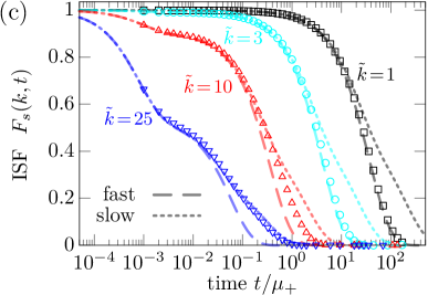
Figure 3: Equilibrium dimer model [$\rho^{\pm}(\tau)$ are both exponential distributions]. The symbols are data obtained by numerical integration of Eqs. (39) and (40). The fast and slow state diffusivities $D_{\pm}$ are set as $D_{+}/D=0.05$ and $D_{-}=0.1D_{+}$, the potential parameter $k_{0}$ as $\beta k_{0}D\mu_{+}=10^{3}$, the mean sojourn time $\mu_{-}$ as $\mu_{-}=\mu_{+}$. (a) MSD vs time. The line is the theoretical prediction in Eq. (59). (b) NGP vs time. The line is the prediction in Eq. (77). (c) ISF vs time. The lines are the predictions in Eqs. (83) (the dashed lines) and (84) (the dotted lines). From right to left, the wave number $k$ is set as $k\sqrt{D\mu_{+}}=1,3,10,25\,(=:\tilde{k})$.

First, let us investigate the case in which the sojourn-time distributions $\rho^{\pm}(\tau)$ are given by the exponential distributions with mean sojourn times $\mu_{\pm}$. Then, equilibrium fractions of the two states are given by

$$p_{\pm}^{\mathrm{eq}}=\frac{\mu_{\pm}}{\mu_{+}+\mu_{-}}.$$ (72)

Initially, the particle is in the fast or the slow state according to the fractions $p_{\pm}^{\mathrm{eq}}$. Then, the Laplace transform of the relaxation function [Eq. (69)] is given by [Eq. (46) in Ref. Miyaguchi et al. (2019)]

$$\mathcal{L}\left[\left\langle e^{-k^{2}\int^{t}_{0}D_{0}(u)du}\right\rangle_{\nu}\right](s)=\frac{z_{+}/\mu_{+}+z_{-}/\mu_{-}+\mathcal{K}^{2}}{\mathcal{K}^{2}[s+D_{0}^{\mathrm{eq}}k^{2}+z_{+}z_{-}/\mathcal{K}]}.$$ (73)

where $\mathcal{K}:=\mu_{+}^{-1}+\mu_{-}^{-1}$, and $z_{\pm}:=s+D_{\pm}k^{2}$. $\mathcal{L}[\dots]$ represents the Laplace transform defined by $\mathcal{L}[g(t)](s):=\int_{0}^{\infty}g(t)e^{-st}dt$. The equilibrium diffusivity $D_{0}^{\mathrm{eq}}$ is here calculated as $D_{0}^{\mathrm{eq}}=p_{+}^{\mathrm{eq}}D_{+}+p_{-}^{\mathrm{eq}}D_{-}$.

For a derivation of the ensemble-averaged MSD and the NGP, a small $k$ limit of the ISF $F_{s}(k,t)$ can be utilized. After a straightforward but slightly lengthy calculation, we obtain

$$\mathcal{L} \left[\left\langle e^{-k^{2}\int^{t}_{0}D_{0}(u)du}\right\rangle_{\nu}\right](s)$$

$$\underset{k\to 0}{\simeq}\frac{1}{s}-\frac{D_{0}^{\mathrm{eq}}k^{2}}{s^{2}}+\frac{(D_{0}^{\mathrm{eq}}k^{2})^{2}}{s^{3}}+\frac{p_{+}^{\mathrm{eq}}p_{-}^{\mathrm{eq}}(\Delta D_{0})^{2}}{s^{2}(s+\mathcal{K})}k^{4},$$ (74)

where $\Delta D_{0}:=D_{+}-D_{-}$. Plugging the Laplace inversion of Eq. (74) into Eq. (69), we obtain the ISF

$$F_{s} (k,t)\underset{k\to 0}{\simeq}$$

$$\exp\left\{-k^{2}[D_{s}(t)+D_{0}^{\mathrm{eq}}]t+\frac{k^{4}p_{+}^{\mathrm{eq}}p_{-}^{\mathrm{eq}}}{2}(\Delta D_{0}t)^{2}g_{d}(\mathcal{K}t)\right\},$$ (75)

where $g_{d}(t)$ is the Debye function defined by Doi and Edwards (1986)

$$g_{d}(t):=\frac{2}{t^{2}}\left(e^{-t}-1+t\right).$$ (76)

Note that Eq. (73) is an exact formula, whereas Eq. (75) and Eq. (82) below are valid only when $D_{\pm}\ll D$, because Eq. (69) was used.

Then, with the relation $\left\langle\!\left\langle\delta\bm{r}^{2}(t)\right\rangle\!\right\rangle_{\nu}=-\nabla_{k}^{2}F_{s}(k,t)|_{k=0}$, it is easy to see that the ensemble-averaged MSD is given by Eq. (59) [or, it is evident because Eq. (75) is a cumulant expansion]. As shown in Fig. 3(a), the prediction is consistent with the simulation. In particular, the MSD exhibits a plateau at the intermediate timescale $1/\nu\ll t\ll 1/\nu_{0}(u)$, which is $10^{-3}\ll t/\mu_{+}\ll 2\times 10^{-2}$ for the parameter values employed in Fig. 3.

Similarly, the NGP $A(t)$ [Eq. (36)] can be derived with $\left\langle\left\langle\delta\bm{r}^{4}\right\rangle\right\rangle_{\nu}=\nabla_{k}^{2}\nabla_{k}^{2}F_{s}(k,t)|_{k=0}$, and we obtain

$$A(t)=\frac{p_{+}^{\mathrm{eq}}p_{-}^{\mathrm{eq}}(\Delta D_{0})^{2}g_{d}(\mathcal{K}t)}{[D_{s}(t)+D_{0}^{\mathrm{eq}}]^{2}}.$$ (77)

As shown in Fig. 3(b), this prediction is also remarkably consistent with numerical simulation. Alternatively, it is also possible to derive Eq. (77) with Eq. (70). In fact, by using Eqs. (17) and (66) in Ref. Miyaguchi et al. (2016), we have the diffusivity correlation as

$$\left\langle\delta D_{0}(t)\delta D_{0}(0)\right\rangle_{\nu}=(\Delta D_{0})^{2}p_{+}^{\mathrm{eq}}p_{-}^{\mathrm{eq}}e^{-\mathcal{K}t}.$$ (78)

Then, substituting Eq. (78) in Eq. (70), we obtain Eq. (77) again.

Next, let us derive the ISF $F_{s}(k,t)$ without the assumption of $k$ being small. To do this, the Laplace inversion of Eq. (73) is carried out as Uneyama et al. (2019)

$$\left\langle e^{-k^{2}\int^{t}_{0}D_{0}(u)du}\right\rangle_{\nu}=A_{+}e^{-\lambda_{+}t}+A_{-}e^{-\lambda_{-}t},$$ (79)

where the relaxation constants $\lambda_{\pm}$ are the simple poles of Eq. (73). $\lambda_{\pm}$ are given by

$$\lambda_{\pm}=\mathcal{K}\frac{1+\frac{D_{+}+D_{-}}{\mathcal{K}}k^{2}\pm\sqrt{1-\frac{2k^{2}}{\mathcal{K}}\Delta p\Delta D_{0}+\left(\frac{k^{2}\Delta D_{0}}{\mathcal{K}}\right)^{2}}}{2},$$ (80)

where $\Delta p:=p_{+}^{\mathrm{eq}}-p_{-}^{\mathrm{eq}}$. Moreover, $A_{\pm}$, the fractions of the two modes, are given by

$$A_{\pm}=\pm\frac{D^{\mathrm{eq}}_{0}k^{2}-\lambda_{\mp}}{\lambda_{+}-\lambda_{-}}.$$ (81)

Note that $A_{+}+A_{-}=1$. Then, by using Eq. (69) and (79), we have the ISF as

$$F_{s}(k,t)=A_{+}e^{-[k^{2}D_{s}(t)+\lambda_{+}]t}+A_{-}e^{-[k^{2}D_{s}(t)+\lambda_{-}]t}.$$ (82)

It is possible to derive Eq. (75) by expanding Eq. (82) with small $k$ up to the fourth order $k^{4}$, thereby obtaining the MSD and NGP again.

There are two extreme cases which are interesting to study: a fast switching limit and a slow switching limit. In the fast switching limit, switching between the two states is faster than the diffusion timescales $1/k^{2}D_{\pm}$, i.e., $\mu_{\pm}\ll 1/k^{2}D_{\pm}$. This is equivalent to take $k\to 0$, and thus from Eq. (75), we have

$$F_{s}(k,t)\underset{k\to 0}{\simeq}\exp\left\{-k^{2}[D_{s}(t)+D_{0}^{\mathrm{eq}}]t\right\}.$$ (83)

Consequently, a single mode relaxation is observed for the fast switching limit $k\to 0$.

The condition for the other extreme case, i.e., the slow switching limit, is given by $\mu_{\pm}\gg 1/k^{2}D_{\pm}$. In this limit, from Eqs. (80) and (81), we have $\lambda_{\pm}\to k^{2}D_{\pm}$ and $A_{\pm}\to p_{\pm}^{\mathrm{eq}}$. Thus, we have from Eq. (79)

$$F_{s}(k,t)\underset{k\to\infty}{\simeq}p_{+}^{\mathrm{eq}}e^{-k^{2}[D_{s}(t)+D_{+}]t}+p_{-}^{\mathrm{eq}}e^{-k^{2}[D_{s}(t)+D_{-}]t}.$$ (84)

This is a simple superposition of the two diffusion processes with diffusivities $D_{\pm}$.

The important point is that, by changing the wave number $k$, the ISF varies between these two extremes [Eqs. (83) and (84)]. Therefore, the ISF might be a very useful tool to elucidate the fluctuating diffusivity Miyaguchi et al. (2019); Dieball et al. (2022). In Fig. 3(c), these two predictions [Eq. (83) and (84)] are compared with simulation. For small $k$, the fast switching limit (the dashed lines) is consistent with the simulation, whereas, for large $k$, the slow switching limit (the dotted lines) is consistent. Moreover, at intermediate values of $k$ [for example, $\tilde{k}=10$ and $25$ in Fig. 3(c)], a two-step relaxation can be observed.

V.2 Power law: Equilibrium ensemble ($1<\alpha<2$)

In this subsection, we assume that the the sojourn-time distribution of the fast state $\rho^{+}(\tau)$ follows the exponential distribution with mean $\mu_{+}$, whereas that of the slow state $\rho^{-}(\tau)$ follows a power-law with index $1<\alpha<2$ and mean $\mu_{-}$ [Eq. (118)]. The equilibrium fractions of the two states are again given by Eq. (72). Moreover, for the equilibrium ensemble, the first sojourn time is chosen from the sojourn-time distribution $\rho^{\pm,\mathrm{eq}}(\tau)$ defined in Eq. (114) instead of $\rho^{\pm}(\tau)$ (See Ref. Miyaguchi et al. (2019) for detail).

Under these conditions, the Laplace transform of the relaxation function in Eq. (69) is given by [Eq. (51) in Ref. Miyaguchi et al. (2019)]

$$\mathcal{L} \left[\left\langle e^{-k^{2}\int^{t}_{0}D_{0}(u)du}\right\rangle_{\nu}\right](s)$$

$$\simeq\frac{1}{s+k^{2}D_{0}^{\mathrm{eq}}}+\frac{a(p_{+}^{\mathrm{eq}}\Delta D_{0})^{2}(s+k^{2}D_{-})^{\alpha-2}k^{4}}{\mu\left(s+k^{2}D_{0}^{\mathrm{eq}}\right)^{2}},$$ (85)

where $\mu:=\mu_{+}+\mu_{-}$, and $a$ is a constant characterizing the power law [Eq. (118)]. This asymptotic relation [Eq. (85)] is valid if the conditions $s\ll 1/\mu_{\pm}$ and $k^{2}D_{\pm}\ll 1/\mu_{\pm}$ are both satisfied Miyaguchi et al. (2019); the latter condition is the fast switching assumption used in the previous subsection.

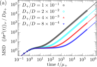
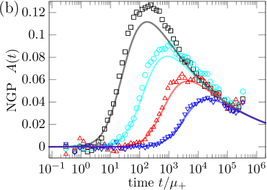
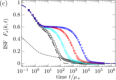
Figure 4: Equilibrium dimer model [$\rho^{+}(\tau)$ and $\rho^{-}(\tau)$ are an exponential distribution and a power law, respectively]. The symbols are data obtained by numerical integration of Eqs. (39) and (40). The fast and slow state diffusivities $D_{\pm}$ are set as $D_{+}/D=10^{-1}$, $2\times 10^{-2}$, $4\times 10^{-3}$, $8\times 10^{-4}$, and $D_{-}=0.01D_{+}$. The power-law index $\alpha$ is fixed as $\alpha=1.2$, the potential parameter $k_{0}$ as $\beta k_{0}D\mu_{+}=1$, the mean sojourn time $\mu_{-}$ as $\mu_{-}=\mu_{+}$, and the cutoff parameter $\tau_{0}$ as $\tau_{0}=\mu_{-}(\alpha-1)/\alpha$ [Eq. (122)]. (a) MSD vs time. The lines are the theoretical prediction in Eq. (59). (b) NGP vs time. The lines are the prediction in Eq. (87). (c) ISF vs time. The lines are the prediction in Eq. (90). The wave number $k$ is set as $k=\sqrt{\beta k_{0}/2}$. [In (b-c), results for the four different values of $D_{+}$ are displayed with the same color code as in (a).].

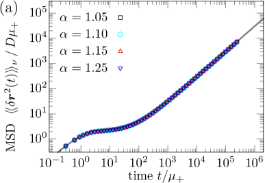
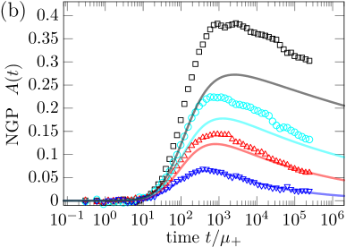
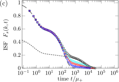
Figure 5: Equilibrium dimer model (the same model as in Fig. 4). The power-law index is set as $\alpha=1.05$, $1.1$, $1.15$ and $1.25$. The diffusivity $D_{\pm}$ of the two states are fixed as $D_{+}/D=3.0\times 10^{-2}$ and $D_{-}=0.01D_{+}$. Parameters $k_{0}$, $\mu_{-}$, $\tau_{0}$, and $k$ are the same as those in Fig. 4. (a) MSD vs time. The line is the theoretical prediction in Eq. (59). (b) NGP vs time. The lines are the prediction in Eq. (87). (c) ISF vs time. The lines are the prediction in Eq. (90). [In (b-c), results for the four different values of $\alpha$ are displayed with the same color code as in (a).

As in the previous subsection, a small $k$ limit of the ISF $F_{s}(k,t)$ is utilized to derive the ensemble-averaged MSD and the NGP. Expanding Eq. (85) around $k=0$, carrying out the Laplace inversion, and inserting the resulting equation into Eq. (69), we obtain

$$F_{s} (k,t)\simeq e^{-k^{2}D_{s}(t)t}$$

$$\times \left[1-k^{2}{D_{0}^{\mathrm{eq}}}t+k^{4}\frac{(D_{0}^{\mathrm{eq}})^{2}t^{2}}{2}+k^{4}\frac{(\Delta D_{0}p_{+}^{\mathrm{eq}})^{2}}{\Gamma(4-\alpha)}\frac{a}{\mu}t^{3-\alpha}\right]$$

$$\simeq \exp\left\{-k^{2}[D_{s}(t)+D_{0}^{\mathrm{eq}}]t+k^{4}\frac{(\Delta D_{0}p_{+}^{\mathrm{eq}})^{2}}{\Gamma(4-\alpha)}\frac{a}{\mu}t^{3-\alpha}\right\}.$$ (86)

Then, with the relation $\left\langle\!\left\langle\delta\bm{r}^{2}(t)\right\rangle\!\right\rangle_{\nu}=-\nabla_{k}^{2}F_{s}(k,t)|_{k=0}$, it is easy to see that the ensemble-averaged MSD is given by Eq. (59). As shown in Figs. 4(a) and 5(a), the theoretical prediction is consistent with the numerical simulations. In particular, the ensemble-averaged MSD shows only normal diffusion and does not depend on the power-law index $\alpha$ as exemplified in Fig. 5(a).

In contrast, non-Gaussianity depends on $\alpha$; in fact, the NGP $A(t)$ [Eq. (36)] can be derived with $\left\langle\left\langle\delta\bm{r}^{4}\right\rangle\right\rangle_{\nu}=\nabla_{k}^{2}\nabla_{k}^{2}F_{s}(k,t)|_{k=0}$ as

$$A(t)\simeq\frac{(\Delta D_{0}\,p_{+}^{\mathrm{eq}})^{2}}{\Gamma(4-\alpha)}\frac{2a}{\mu}\frac{t^{1-\alpha}}{\left(1/\beta k_{0}t+D_{0}^{\mathrm{eq}}\right)^{2}},$$ (87)

where the short-time diffusivity $D_{s}(t)$ is replaced with its asymptotic form at long times $D_{s}(t)\simeq 1/\beta k_{0}t$, because Eq. (85) is valid only for large $t$ (i.e., $t\gg\mu_{\pm}$). The above formula [Eq. (87)] can be also derived through Eq. (70) with the correlation function of diffusivity [Eq.(111) in Ref. Miyaguchi et al. (2016)]

$$\left\langle\delta D_{0}(t)\delta D_{0}(0)\right\rangle_{\nu}\simeq\frac{(\Delta D_{0}\,p_{+}^{\mathrm{eq}})^{2}}{\Gamma(2-\alpha)}\frac{a}{\mu}t^{1-\alpha}.$$ (88)

As shown in Fig. 4(b) and 5(b), both of the theory and simulations of the NGP $A(t)$ show unimodal structures, but around the peaks, there are systematic deviations; for $\alpha$ closer to unity, the deviation is more serious. Therefore, these deviations might be attributed to the higher order corrections neglected in Eq. (85). At long times, the theoretical prediction is consistent with the numerical simulations (as it should be) except for the case $\alpha=1.05$; for $\alpha=1.05$, the simulation time might well be shorter than the time scale at which the asymptotic relation [Eq. (87)] becomes precise.

Finally, a formula for the ISF is derived without the assumption of $k$ being small. The Laplace inversion of Eq. (85) gives [Eqs. (53) and (55) in Ref. Miyaguchi et al. (2019)]

$$\left\langle e^{-k^{2}\int^{t}_{0}D_{0}(u)du}\right\rangle_{\nu}$$

$$\simeq\begin{cases}e^{-k^{2}D_{0}^{\mathrm{eq}}t}&(t\sim\frac{1}{D_{+}k^{2}}),\\[2.84544pt] \frac{a}{\mu}\left(\frac{p_{+}^{\mathrm{eq}}\Delta D_{0}}{D_{0}^{\mathrm{eq}}}\right)^{2}\frac{e^{-k^{2}D_{-}t}t^{1-\alpha}}{{\color[rgb]{0,0,0}|\Gamma(2-\alpha)|}}&(t\gg\frac{1}{D_{+}k^{2}}).\end{cases}$$ (89)

By using Eqs. (69) and (89), the ISF is given by

$$F_{s}(k,t)\simeq\begin{cases}e^{-k^{2}[D_{0}^{\mathrm{eq}}+D_{s}(t)]t}&(t\sim\frac{1}{D_{+}k^{2}}),\\[2.84544pt] \frac{a}{\mu}\left(\frac{p_{+}^{\mathrm{eq}}\Delta D_{0}}{D_{0}^{\mathrm{eq}}}\right)^{2}\frac{e^{-k^{2}[D_{s}(t)+D_{-}]t}t^{1-\alpha}}{{\color[rgb]{0,0,0}|\Gamma(2-\alpha)|}}&(t\gg\frac{1}{D_{+}k^{2}}).\end{cases}$$ (90)

As show in Fig. 4(c) with dashed lines, the first of these functions shows two-step relaxation. There is a plateau between the two relaxation steps, and the duration of the plateau becomes longer for smaller diffusivity $D_{+}$.

In Figs. 4(c) and 5(c), the theoretical prediction [the first equation in Eq. (90)] is compared with the numerical simulation. The theoretical prediction (the dashed lines) is consistent with the numerical simulation (symbols) except at long times, at which the second equation in Eq .(90) shows good agreement [to avoid complication, the second equation is shown by dotted lines only for the cases $D_{+}/D=0.1$ in Fig. 4(c) and $\alpha=1.05$ in Fig. 5(c)]. In simulations, the wave number $k$ is set as $k=\sqrt{\beta k_{0}/2}$, the inverse of which, $\sqrt{2/\beta k_{0}}$, is a characteristic size of the harmonic potential since $2D_{s}(t)t\to 2/\beta k_{0}$ as $t\to\infty$ Fodor et al. (2016).

Finally, it is worth commenting that the formulas for the MSD [Eq.(59)] and the ISF [Eq. (90)] are valid even for the case $\alpha>2$ Miyaguchi et al. (2019). In contrast, the NGP formula in Eq. (87) is no more valid for $\alpha>2$, and it should be necessary to include a leading term correctly.

V.3 Power law: Non-equilibrium ensemble ($0<\alpha<1$)

Next, we investigate the case in which the sojourn time distribution $\rho^{-}(\tau)$ is a power-law with $0<\alpha<1$. In this case, there is no equilibrium state, because the mean sojourn time for this power-law distribution does not exist. Therefore, we employ a typical non-equilibrium ensemble as an initial ensemble, for which the first sojourn time simply follows $\rho^{-}(\tau)$ Miyaguchi et al. (2016, 2019). The sojourn-time distribution for the fast state $\rho^{+}(\tau)$ is again assumed to be the exponential distribution with mean $\mu_{+}$. Furthermore, the initial fractions $p_{\pm}^{0}$ ($p_{+}^{0}+p_{-}^{0}=1$) for the two states are necessary for specifying the initial ensemble. However, the results obtained below for large $t$ are independent of $p_{\pm}^{0}$.

Under these conditions, the Laplace transform of the relaxation function in Eq. (69) is given by [Eq. (62) in Ref. Miyaguchi et al. (2019)]

$$\mathcal{L}\left[\left\langle e^{-k^{2}\int^{t}_{0}D_{0}(u)du}\right\rangle_{\nu}\right](s)\simeq$$

$$\frac{1}{z_{-}}-\frac{\mu_{+}k^{2}\Delta D_{0}}{az_{-}^{1+\alpha}}+\frac{\mu_{+}^{2}k^{2}\Delta D_{0}z_{+}}{a^{2}z_{-}^{1+2\alpha}}+\frac{p_{-}^{0}\mu_{+}k^{2}\Delta D_{0}}{az_{-}},$$ (91)

where $z_{\pm}:=s+k^{2}D_{\pm}$. In Ref. Miyaguchi et al. (2019), the last two terms on the right-hand side of Eq. (91) are not taken into account, but terms up to $k^{4}$ are necessary to obtain the NGP [The derivation procedure of Eq. (91) is the same as that of Eq.(62) in Ref. Miyaguchi et al. (2019)]. In a derivation of Eq. (91), the fast switching assumption for the fast state $k^{2}D_{+}\ll 1/\mu_{+}$ as well as a similar condition for the slow state $k^{2}D_{-}\ll 1/a^{1/\alpha}$ are assumed. Similarly, it is also supposed that $s$ satisfies $s\ll 1/\mu_{+}$ and $s\ll 1/a^{1/\alpha}$ Miyaguchi et al. (2019).

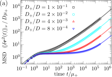
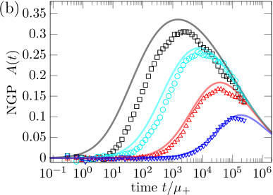
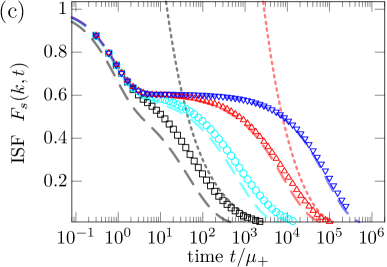
Figure 6: Non-equilibrium dimer model [$\rho^{+}(\tau)$ and $\rho^{-}(\tau)$ are an exponential distribution and a power law, respectively]. The symbols are data obtained by numerical integration of Eqs. (39) and (40). The fast and slow state diffusivities $D_{\pm}$ are set as $D_{+}/D=10^{-1},2\times 10^{-2},4\times 10^{-3},8\times 10^{-4}$, and $D_{-}=0.01D_{+}$. The power-law index $\alpha$ is fixed as $\alpha=0.6$, the potential parameter $k_{0}$ as $\beta k_{0}D\mu_{+}=1$, the initial fractions $p_{\pm}^{0}$ as $p_{\pm}^{0}=0.5$, and the cutoff parameter $\tau_{0}$ as $\tau_{0}/\mu_{+}=0.1$. (a) MSD vs time. The lines are the theoretical prediction in Eq. (93). (b) NGP vs time. The lines are the prediction in Eq. (87). (c) ISF vs time. The lines are the prediction in Eq. (98). The wave number $k$ is set as $k=\sqrt{\beta k_{0}/2}$. [In (b-c), results for the four different values of $D_{+}$ are displayed with the same color code as in (a)].

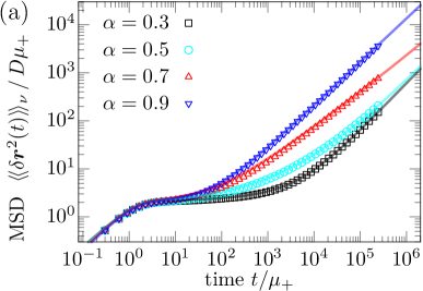
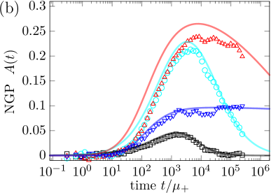
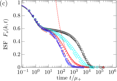
Figure 7: Non-equilibrium dimer model (the same model as in Fig. 6). The power-law index is set as $\alpha=0.3,0.5,0.7$ and $0.9$. The diffusivity $D_{\pm}$ of the two states are fixed as $D_{+}/D=3.0\times 10^{-2}$ and $D_{-}=0.01D_{+}$. Parameters $k_{0}$, $p_{\pm}^{0}$, $\tau_{0}$, and $k$ are the same as those in Fig. 6. (a) MSD vs time. The lines are the theoretical prediction in Eq. (93). (b) NGP vs time. The lines are the prediction in Eq. (96). (c) ISF vs time. The lines are the prediction in Eq. (98). [In (b-c), results for the four different values of $\alpha$ are displayed with the same color code as in (a)].

To obtain the MSD and the NGP, we derive the ISF at small $k$. We expand Eq. (91) around $k=0$, and carry out the Laplace inversion; the resulting equation is substituted in Eq. (69), thereby obtaining the ISF at small $k$

$$F_{s}(k,t)\simeq e^{-k^{2}D_{s}(t)t}$$

$$\times\left[1-k^{2}(At^{\alpha}+D_{-}t)+\frac{k^{4}(At^{\alpha}+D_{-}t)^{2}}{2}+\frac{k^{4}A^{2}Bt^{2\alpha}}{2}\right]$$

$$\simeq\exp\left\{-k^{2}\left[D_{s}(t)+At^{\alpha-1}+D_{-}\right]t+\frac{k^{4}A^{2}Bt^{2\alpha}}{2}\right\},$$ (92)

where we omit some lower order terms with respect to $t$; $A$ and $B$ are constants defined as $A:=\mu_{+}\Delta D_{0}/a\Gamma(1+\alpha)$ and $B=2\Gamma^{2}(1+\alpha)/\Gamma(1+2\alpha)-1$.

By using $\left\langle\!\left\langle\delta\bm{r}^{2}(t)\right\rangle\!\right\rangle_{\nu}=-\nabla_{k}^{2}F_{s}(k,t)|_{k=0}$, we obtain the ensemble-averaged MSD as

$$\frac{\left\langle\left\langle\delta\bm{r}^{2}(t)\right\rangle\right\rangle_{\nu}}{2n}\simeq\left[D_{s}(t)+At^{\alpha-1}+D_{-}\right]t.$$ (93)

This formula is evident again from the fact that Eq. (92) is a cumulant expansion. Alternatively, the MSD formula can be derived with Eq. (58). In fact, from Eqs. (30) and (87) in Ref. Miyaguchi et al. (2016), we have $\langle D_{0}(u)\rangle_{\nu}\simeq\alpha At^{\alpha-1}+D_{-}$. With this relation and Eq. (58), we recover Eq. (93).

In contrast to the equilibrium ensemble, in which only normal diffusion is observed, the MSD for the non-equilibrium ensemble shows transient subdiffusion at intermediate timescale. At longer timescale, normal diffusion recovers (the long-time diffusivity is $D_{-}$). Interestingly, the same intermediate and long-time properties as in Eq. (93) are observed in a molecular dynamics simulation for supercooled liquids Kob and Andersen (1995a). As shown in Figs. 6(a) and 7(a), the theoretical prediction in Eq. (93) is consistent with numerical simulations, except for the case $D_{+}/D=0.1$. The slight inconsistency for $D_{+}/D=0.1$ should be caused by the assumption $D_{+}\ll D$, which is used in our analysis [See the text above Eq. (54)].

As remarked in Sec. IV.2, the ensemble-averaged and time-averaged MSDs do not coincide in non-equilibrium systems. Therefore, here a formula for the time-averaged MSD is derived by using the general expression in Eq. (66). The mean diffusivity $\left\langle D_{0}(t)\right\rangle_{\nu}$ is given by [Eqs.(30) and (87) in Ref.Miyaguchi et al. (2016)]

$$\left\langle D_{0}(t)\right\rangle_{\nu}\approx D_{-}+\Delta D_{0}\frac{\mu_{+}t^{\alpha-1}}{a\Gamma(\alpha)}.$$ (94)

Thus, $D_{0}(t)$ is a non-stationary process; the origin of the non-stationarity can be understood from the fact that the diffusive state is increasingly stuck in the slow state $D_{-}$ as $t$ increases Korabel and Barkai (2010); Miyaguchi et al. (2016).

Inserting Eq. (94) into Eq. (67), we obtain an explicit formula for $\left\langle\overline{D}_{0}(u;t)\right\rangle_{\nu}$. Then, substituting this formula into Eq. (66), we have the ensemble average of the time-averaged MSD as

$$\frac{\left\langle\left\langle\overline{\delta\bm{r}}^{2}(\Delta;t)\right\rangle\right\rangle_{\nu}}{2n}\simeq\left[D_{s}(\Delta)+At^{\alpha-1}+D_{-}\right]\Delta,$$ (95)

where $\Delta\ll t$ is assumed. Thus, the time-averaged MSD has a form different from the ensemble-averaged one [Eq. (93)]; this is a natural consequence of the non-stationarity of $D_{0}(t)$ [Eq. (94)].

In particular, the time-averaged MSD does not exhibit subdiffusion in contrast to the ensemble-averaged MSD. It is also prominent that the time-averaged MSD depends on the measurement time $t$; such a property is referred to as an aging effect Schulz et al. (2014). This aging effect occurs at an intermediate timescale (with respect to the measurement time $t$), at which the ensemble-averaged MSD shows the subdiffusion.

In Fig. 8, time dependences of the ensemble-averaged MSD [Eq. (93)] and the ensemble average of the time-averaged MSD [Eq. (95)] are displayed with thick solid and dashed lines. It is clear that these two MSDs behave differently at the intermediate timescale. In contrast, at short and long times, these two MSDs coincide.

Moreover, in Fig. 8, numerical results of the time-averaged MSDs are also presented with thin red lines; each red line is calculated from a single trajectory data. It is clear that the time-averaged MSDs show trajectory-to-trajectory fluctuations. Relaxation properties of these fluctuations should be closely related to non-Gaussianity of displacement distributions Miyaguchi et al. (2016).

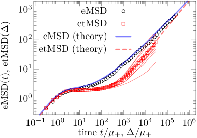
Figure 8: Ensemble-averaged and time-averaged MSDs vs time for non-equilibrium dimer model (the same model as in Fig. 6). The thick solid line and the thick dashed line are the theoretical predictions for the ensemble-averaged MSD [Eq. (93)] and the ensemble average of time-averaged MSD [Eq. (95)], respectively. Each thin red solid line is a time-averaged MSD obtained from a single trajectory data; time-averaged MSDs for ten trajectories are displayed. The power-law index and the total measurement time are set as $\alpha=0.7$ and $t=3\times 10^{5}$. The other parameters $D_{\pm}$, $k_{0}$, $p_{\pm}^{0}$ and $\tau_{0}$ are the same as those in Fig. 7.

In the same way as the ensemble-averaged MSD, the NGP [Eq. (36)] can be derived with $\left\langle\left\langle\delta\bm{r}^{4}\right\rangle\right\rangle_{\nu}=\nabla_{k}^{2}\nabla_{k}^{2}F_{s}(k,t)|_{k=0}$ as

$$A(t)\simeq\frac{A^{2}Bt^{2\alpha-2}}{\left(1/\beta k_{0}t+D_{-}+At^{\alpha-1}\right)^{2}},$$ (96)

where the short-time diffusivity $D_{s}(t)$ is replaced with its asymptotic form at long times $D_{s}(t)\simeq 1/\beta k_{0}t$, because Eq. (91) is valid only for large $t$ (i.e., $t\gg\mu_{\pm},\,a^{1/\alpha}$). This function shows a unimodal shape as shown in Figs. 6(b) and 7(b), in which Eq. (96) is compared with the simulations. The agreement is fairly good, but there are some deviations, which might be due to lower order corrections neglected in deriving Eq. (92).

Next, let us derive a formula for the ISF $F_{s}(k,t)$ without the assumption of $k$ being small. With the Laplace inversion of the first and second terms of Eq. (91) (the third and fourth terms are neglected, because they are lower order corrections in terms of $t$), the relaxation function is given by [Eqs. (63) and (65) in Ref. Miyaguchi et al. (2019)]

$$\left\langle e^{-k^{2}\int^{t}_{0}D_{0}(u)du}\right\rangle_{\nu}\simeq\begin{cases}e^{-k^{2}\left[D_{-}+At^{\alpha-1}\right]t},&(t\sim\frac{1}{D_{+}k^{2}}),\\[2.84544pt] \frac{\Delta D_{0}}{k^{2}D_{+}^{2}}\frac{a}{\mu_{+}}\frac{e^{-k^{2}D_{-}t}}{\Gamma(1-\alpha)t^{\alpha}},&(t\gg\frac{1}{D_{+}k^{2}}).\end{cases}$$ (97)

By using Eqs. (69) and (97), the ISF is obtained as

$$F_{s}(k,t)\simeq\begin{cases}e^{-k^{2}\left[D_{s}(t)+D_{-}+At^{\alpha-1}\right]t},&(t\sim\frac{1}{D_{+}k^{2}}),\\[2.84544pt] \frac{\Delta D_{0}}{k^{2}D_{+}^{2}}\frac{a}{\mu_{+}}\frac{e^{-k^{2}[D_{s}(t)+D_{-}]t}}{\Gamma(1-\alpha)t^{\alpha}},&(t\gg\frac{1}{D_{+}k^{2}}),\end{cases}$$ (98)

which shows an exponential relaxation at short time, a stretched-exponential relaxation at intermediate time, and a power-law relaxation at long time.

As in the equilibrium case, the first equation in Eq. (98) exhibits a two-step relaxation as shown in Figs. 6(c) and 7(c). The theoretical prediction (the dashed lines) is consistent with the numerical simulation except at long time, at which the second equation in Eq . (98) shows good agreement [the second equation is shown by dotted lines only for the cases $D_{+}/D=10^{-1}$ and $4\times 10^{-3}$ in Fig. 6(c) and $\alpha=0.7$ in Fig. 7(c)].

VI Discussion

Several models with both the memory effect and the fluctuating diffusivity have been proposed and studied so far Ślęzak et al. (2018); Wang et al. (2020a, b); Sabri et al. (2020); Janczura et al. (2021); Dieball et al. (2022); Goswami and Chakrabarti (2022), but physical backgrounds of these models, such as the fluctuation-dissipation relation, have been unclear. In this paper, we proposed the GLEFD [Eq. (20)], and showed that it satisfies the generalized fluctuation-dissipation relation [Eq. (21)]. By utilizing the Markovian embedding method, a numerical integration scheme of the GLEFD was also presented. With the physical background, the GLEFD [Eqs. (20) and (21)] should become an important model to explain complex diffusion processes observed in single-particle-tracking experiments and molecular dynamics simulations.

To explain the non-Gaussianity in the viscoelastic dynamics, a random potential energy (quenched disorder) has also been frequently employed Goychuk and Pöschel (2020); Goychuk and Pöschel (2021). It is probable that such an approach is related to the one presented in this article, because quenched disorder can be approximated with annealed disorder for some systems with dimension higher than two Machta (1985); Bouchaud (1992), and the annealed disorder might be modeled by the fluctuating diffusivity Uneyama et al. (2015). It is also worth noticing that annealed models are easier to handle theoretically than quenched models Bouchaud and Georges (1990).

Moreover, as special cases of the GLEFD, the FBMFD and the dimer model were investigated in detail. The FBMFD, which shows the subdiffusion, non-Gaussianity and stretched-exponential relaxation, must be an important model in biological applications. This is because subdiffusion and non-Gaussianity are observed in many single-particle-tracking experiments inside cytoplasm He et al. (2008); Parry et al. (2014); Lampo et al. (2017); Sabri et al. (2020); Janczura et al. (2021) and molecular dynamics simulations Akimoto et al. (2011); Yamamoto et al. (2014); Jeon et al. (2016); Yamamoto et al. (2017); importantly, in some experiments and simulations, the subdiffusion is attributed to the FBM-like anti-persistent correlation Magdziarz et al. (2009); Thapa et al. (2018); Lampo et al. (2017); Akimoto et al. (2011); Jeon et al. (2016). The origin of the non-Gaussianity is still controversial, but, in our approach, it is attributed to the fluctuating diffusivity.

In the FBMFD in this article, the power-law index $\alpha$ is constant, whereas some experiments have revealed that this parameter is also random Sabri et al. (2020); Janczura et al. (2021). To incorporate a time-dependent fluctuation in $\alpha$ in our approach, $k_{i}$ in Eq. (14) should be fluctuating and depend on time. This however causes a violation of the detailed balance, because the potential energy changes with time. Thus, it is an interesting question whether equilibrium dynamics can or cannot explain the randomness in the power-law index $\alpha$.

The dimer model is one of the simplest model of the GLEFD, and analytically tractable to some extent. In fact, only this case can be described by a single equation without an integral term [Eq. (45)], with which we can see a complicated interplay between the memory effect and the fluctuating diffusivity [Eq. (47)]. Formulas for the MSD, the NGP, and the ISF in the dimer model were also derived analytically, and it was found that they are fairly consistent with numerical simulations. In particular, for the non-equilibrium ensemble, the dimer model exhibits subdiffusion as well as stretched-exponential relaxation at intermediate timescales.

Both the FBMFD and the non-equilibrium dimer model show subdiffusion, non-Gaussianity (with a unimodal shape in the NGP), and stretched-exponential relaxation. In addition to these features, the dimer model also exhibits plateaus in the MSD and the ISF; these features are similar to those observed in supercooled liquids and glassy systems Götze (2009). However, it is numerically reported in Ref. Kob and Andersen (1995a, b) that these properties are observed even in equilibrium systems. In contrast, for the dimer model, subdiffusion and stretched-exponential relaxation are observed only for the non-equilibrium initial conditions, and thus the mechanism giving rise to the above properties in the dimer model might well be different from that in the supercooled liquids and glassy systems.

Note however that we only studied the fast switching limit for the dimer model with power-law sojourn times. For the case in which timescales of switching and diffusion are comparable, analytical results are limited to the equilibrium dimer model in which the sojourn-time distributions $\rho^{\pm}(\tau)$ are both given by exponential distributions [Fig. 3]. Thus, an interesting question for future studies would be to clarify the properties without the fast switching assumption. In addition, throughout the analysis of the dimer model [Secs. IV and V], we assume $D_{0}(t)\ll D$; it should be also important to study the dimer model without this assumption.

To incorporate the fluctuating diffusivity into the GLE, we used the Markovian embedding in this paper, but there should be other ways to do so. For example, it is possible to incorporate it by assuming that the memory is reset at each switching event. There would be some situations in which resetting the memory is a natural choice Dieball et al. (2022), though evolution equations without resetting (such as the GLEFD in this article) might be more natural in other situations; an example is monomer dynamics of a flexible polymer, in which the memory effect originates from internal degrees of freedom of the polymer Panja (2010), and the fluctuating diffusivity originates from hydrodynamic interactions Miyaguchi (2017); Yamamoto et al. (2021) or polymer size fluctuations Nampoothiri et al. (2021, 2022).

But, whether it is possible to derive the GLEFD from microscopic models such as polymer systems should be explored in future studies. Because the GLE is derived from microscopic equations of motion with the projection operator method Götze (2009); Hansen and McDonald (1990), and thus the auxiliary variables should be related to the fast variables which are projected out. For example, the middle monomer of the Rouse polymer can be described by Eqs. (13) and (14), where the auxiliary variables $\bm{r}_{i}(t)$ are normal modes of the Rouse polymer Panja (2010). If the hydrodynamic interactions between the monomers are further taken into account, the diffusivities of the normal modes might be fluctuating Miyaguchi (2017). These points will be investigated in more detail and reported elsewhere.

Although the GLEFD is constructed in the presence of the external force $\bm{F}_{e}$ [Eq. (20)], the FBMFD and the dimer model were studied in the absence of $\bm{F}_{e}$. Thus, effects of external forces such as a constant force and a force due to a harmonic potential should be explored in future work. Moreover, beyond the analysis of the NGP, elucidation of displacement distributions for the GLEFD is also an important future subject Lanoiselée and Grebenkov (2018); Barkai and Burov (2020); Hidalgo-Soria et al. (2021). A quantity called codifference may also be useful to characterize the non-Gaussianity Ślęzak et al. (2019).

Fluctuation properties of the time-averaged MSD are not elucidated in this work, but such properties are quite important in that they are closely related to the non-Gaussianity of the displacement, and that fluctuation analysis of the time-averaged MSD would be more efficient than the NGP method Miyaguchi (2017); Yamamoto et al. (2021). Fluctuation properties of the time-averaged MSD have been studied with its relative standard deviation or relative variance (the latter is referred to as an ergodicity breaking parameter Metzler et al. (2014)). For normal diffusion with fluctuating diffusivity, such parameters have been shown to behave similarly to the NGP $A(t)$ at long times Miyaguchi et al. (2016), but further studies are necessary for subdiffusive systems.

In this article, the fluctuating diffusivity is assumed to be a scalar. But, many diffusion processes are described by diffusivity given by a second rank tensor Dhont (1996); Miyaguchi (2017). Therefore, a generalization to the tensor diffusivity should be studied in future. Moreover, in all the simulations in this article, the fluctuating diffusivity is assumed to be two-state processes. Instead of these two-state processes, it is interesting to use a process of which stationary distribution is consistent with experimentally observed distributions such as the exponential distribution Lampo et al. (2017); Chechkin et al. (2017); Lanoiselée and Grebenkov (2018).

In GLEFD [Eq. (20)], the fluctuating diffusivity is incorporated only into the correlated noise $\bm{\xi}_{c}(t)$ and the white Gaussian noise $\bm{\xi}(t)$ is left unchanged. But, it is also interesting to study the opposite case in which the diffusivity due to the white noise $\bm{\xi}(t)$ is fluctuating and that due to the correlated noise $\bm{\xi}_{c}(t)$ is not fluctuating. Such a model might be relevant for tagged-particle motion in single-file diffusion Kollmann (2003) with wall effects Alexandre et al. (2022). Furthermore, we studied the GLEFD at the overdamped limit, but it is also possible to incorporate the fluctuating diffusivity into the underdamped GLE Goychuk (2009).

The procedure used to obtain the FBMFD is readily generalized into an arbitrary memory kernel. In fact, if an even function $\phi(t)$ is a memory kernel of a GLE without the fluctuating diffusivity and the property in Eq. (30) is assumed, then the memory kernel $\phi(t,t^{\prime})$ of the corresponding GLEFD is given by

$$\phi(t,t^{\prime})=\phi\left(\int_{t^{\prime}}^{t}\kappa(u)du\right).$$ (99)

Note that Eqs. (27) and (32) satisfy the above relation.

Unfortunately, it is difficult at present to theoretically analyze the GLEFD, because the integral term of the GLEFD [Eq. (20)] is not of a convolution form and consequently the Laplace transform cannot be utilized [Note also that, in spite of this non-convolution form, the time-translation symmetry is not broken, if the system is in equilibrium. See Eq. (23)]. Hence, developing theoretical tools, which includes an approach through Fokker–Planck-like equations Fox (1977), to analyze the GLEFD should be one of the most important future tasks.

It is interesting to examine whether the generalized fluctuation-dissipation relation in Eq. (21) is valid in more general diffusivity fluctuations. For example, suppose that the correlated noise $\bm{\xi}_{c}(t)$ in the GLEFD [Eq. (20)] is given by

$$\bm{\xi}_{c}(t)=B(t)\bm{\xi}_{c}^{0}(t),$$ (100)

where $B(t)$ is a stochastic process, and $\bm{\xi}_{c}^{0}(t)$ is a correlated Gaussian noise [a similar system was studied in Refs. Wang et al. (2020a, b) without the integral term and the white noise $\bm{\xi}(t)$]. Then, it is tempting to conjecture from Eq. (21) that the fluctuation-dissipation relation would be given by

$$\phi(t,t^{\prime})\bm{I}=\left\langle\bm{\xi}_{c}(t)\bm{\xi}_{c}(t^{\prime})\right\rangle=B(t)B(t^{\prime})\left\langle\bm{\xi}_{c}^{0}(t)\bm{\xi}_{c}^{0}(t^{\prime})\right\rangle.$$ (101)

It is possible to show that the conjecture is true with a Markovian embedding method. In fact, the Markovian embedding in Sec. II.2 can be utilized again except Eq. (12), which is replaced with

$$k_{i}^{\prime}(\bm{r}_{i}-\bm{r})=\sqrt{D}\bm{\xi}_{i}-k_{i}^{\prime}\int_{0}^{t}e^{-\nu_{i}(t-t^{\prime})}B(t^{\prime})\dot{\bm{r}}(t^{\prime})dt^{\prime}.$$ (102)

Then, Markovian equations of motion are obtained as

$$\frac{d\bm{R}(t)}{dt}=\beta\bm{L}\cdot\bm{F}+\bm{\Xi},$$ (103)

where a supervector notation $\bm{R}(t):=(\bm{r},\bm{r}_{0},\dots,\bm{r}_{N-1})$ is employed

In Eq. (103), $\beta\bm{L}$ is a mobility tensor defined by

$$\bm{L}=\begin{pmatrix}D\bm{I}&DC\bm{I}&\dots&DC^{2}\bm{I}\\ DC\bm{I}&(D_{0}+DC^{2})\bm{I}&\dots&DC^{2}\bm{I}\\ \vdots&&&\\ DC\bm{I}&DC^{2}\bm{I}&\dots&(D_{N-1}+DC^{2})\bm{I}\\ \end{pmatrix},$$ (104)

where $C(t):=1-B(t)$. Moreover, $\bm{F}$ is a (non-random) force vector given by $\bm{F}:=(\bm{F}_{t}+\bm{F}_{e},\bm{F}_{0},\dots,\bm{F}_{N-1})$. Here, $\bm{F}_{i}$ are harmonic forces exerted on the auxiliary variables $\bm{r}_{i}$ and are defined by $\bm{F}_{i}:=k_{i}(\bm{r}-\bm{r}_{i})$; and $\bm{F}_{t}$ is a resultant force exerted on the original variable $\bm{r}$ and is defined by $\bm{F}_{t}:=-\sum_{i=0}^{N-1}\bm{F}_{i}$. Finally, $\bm{\Xi}$ is a noise vector defined by

$$\bm{\Xi}=\begin{pmatrix}\sqrt{2D}\bm{\xi}\\ \sqrt{2D}C\bm{\xi}+\sqrt{2D_{0}}\bm{\eta}_{0}\\ \vdots\\ \sqrt{2D}C\bm{\xi}+\sqrt{2D_{N-1}}\bm{\eta}_{N-1}\\ \end{pmatrix},$$ (105)

where $\bm{\eta}_{i}(t)$ is the white Gaussian noise defined in Eq. (9). If $C(t)\equiv 0$, Eq. (103) is equivalent to Eqs. (13) and (14).

Then, it is readily shown that Eq. (103) satisfies the fluctuation-dissipation relation $\left\langle\bm{\Xi}(t)\bm{\Xi}(t^{\prime})\right\rangle=2\bm{L}\delta(t-t^{\prime})$ Doi and Edwards (1986). Thus, a generality of Eq. (21) should be promising, but further studies are obviously required. Moreover, it should be interesting per se to study the GLEFD [Eq. (20)] with Eqs. (100) and (101). Note that Eq. (103) can be utilized as a scheme for numerical integration of this system.

Appendix A Fractional Brownian motion

In this Appendix, the FBM without the fluctuating diffusivity [Eqs. (24) and (25)] is briefly reviewed. Carrying out the double Laplace transforms ($t\leftrightarrow s$ and $t^{\prime}\leftrightarrow s^{\prime}$) of Eqs. (5) and (6), we have fluctuation-dissipation relations in the Laplace domain Pottier (2003)

$$\Bigl{\langle}\hat{\bm{\xi}}(s)\hat{\bm{\xi}}(s^{\prime})\Bigr{\rangle} =\frac{1}{s+s^{\prime}}\bm{I},$$ (106)

$$\left\langle\hat{\bm{\xi}}_{c}^{0}(s)\hat{\bm{\xi}}_{c}^{0}(s^{\prime})\right\rangle =\frac{\hat{\phi}(s)+\hat{\phi}(s^{\prime})}{s+s^{\prime}}\bm{I}.$$ (107)

Moreover, the Laplace transform of Eq. (24) is given by

$$\hat{\bm{r}}(s)=\sqrt{D}\frac{\sqrt{2}\hat{\bm{\xi}}(s)+\hat{\bm{\xi}}_{c}(s)}{s[1+\hat{\phi}(s)]}$$ (108)

where $\bm{r}(0)=0$ is assumed, and consequently $\delta\bm{r}(t)=\bm{r}(t)$ in the following. With these relations and the independence of $\hat{\bm{\xi}}$ and $\hat{\bm{\xi}}_{c}^{0}$, we obtain

$$\left\langle\hat{\bm{r}}(s)\hat{\bm{r}}(s^{\prime})\right\rangle=D\frac{\frac{1}{1+\hat{\phi}(s)}+\frac{1}{1+\hat{\phi}(s^{\prime})}}{ss^{\prime}(s+s^{\prime})}\bm{I},$$ (109)

If the memory kernel $\phi(t)$ is the power-law form in Eq. (25), its Laplace transform is given by $\hat{\phi}(s)=A\Gamma(1-\alpha)s^{\alpha-1}$ $(0<\alpha<1)$. Using this relation and Eq. (109), we obtain

$$\left\langle\hat{\bm{r}}(s)\hat{\bm{r}}(s^{\prime})\right\rangle\simeq\begin{cases}\frac{2D}{ss^{\prime}(s+s^{\prime})}\bm{I},&[1\ll\hat{\phi}(s),\hat{\phi}(s^{\prime})],\\[2.84544pt] \frac{D_{\alpha}\Gamma(1+\alpha)(s^{1-\alpha}+s^{\prime 1-\alpha})}{ss^{\prime}(s+s^{\prime})}\bm{I},&[1\gg\hat{\phi}(s),\hat{\phi}(s^{\prime})].\end{cases}$$ (110)

Then, the double Laplace inversions give the following asymptotic formulas at short and long times:

$$\left\langle\bm{r}(t)\bm{r}(t^{\prime})\right\rangle\simeq\begin{cases}{2D}\mathrm{min}(t,t^{\prime})\bm{I},&(t,t^{\prime}\ll t_{c}),\\[2.84544pt] D_{\alpha}[t^{\alpha}+t^{\prime\alpha}-|t-t^{\prime}|^{\alpha}]\bm{I},&(t,t^{\prime}\gg t_{c}),\end{cases}$$ (111)

where $t_{c}:=[\Gamma(1+\alpha)D_{\alpha}/D]^{1/(1-\alpha)}$ is the crossover time. By putting $t=t^{\prime}$ and taking contractions of the tensors, we obtain the MSD in Eq. (26).

Likewise, for the case in which $t^{\prime}\ll t_{c}\ll t$, we have $\langle\bm{r}(t)\bm{r}(t^{\prime})\rangle\simeq D_{\alpha}[t^{\alpha}-(t-t^{\prime})^{\alpha}]$. Autocorrelation of the velocity $\bm{v}(t):=d\bm{r}(t)/dt$ is obtained by differentiating the above equation with $t$ and $t^{\prime}$ and then putting $t^{\prime}=0$ as $\langle\bm{v}(t)\bm{v}(0)\rangle\simeq\alpha(\alpha-1)t^{\alpha-2}\bm{I}$ for $t\gg t_{c}$. Thus, the velocity shows negative (anti-persistent) correlation at long times.

Appendix B Exact MSD formula for dimer model

For the dimer model, a formula for the MSD [Eq. (59)] is derived under the assumption $D_{0}(t)\ll D$ for any $t$. But, if $D_{0}(t)$ is a stationary process, it is also possible to derive an exact formula as shown below. Let us study the two-state model in which the sojourn-time distributions $\rho^{\pm}(\tau)$ are exponential distributions. From Eqs. (53) and (79), we have

$$\frac{f(t)}{D\beta k_{0}}=A_{+}e^{-(\beta k_{0}D+\lambda_{+})t}+A_{-}e^{-(\beta k_{0}D+\lambda_{-})t},$$ (112)

where $k^{2}$ in $\lambda_{\pm}$ [Eq. (80)] and $A_{\pm}$ [Eq. (81)] should be replaced with $\beta k_{0}$.

Then, the MSD can be calculated with Eqs. (52) and (112) as

$$\frac{\left\langle\left\langle\delta\bm{r}^{2}(t)\right\rangle\right\rangle_{\nu}}{2n}=D\left[t-\frac{\beta k_{0}D}{2}t^{2}\sum_{l=\pm}A_{l}g_{d}((\beta k_{0}D+\lambda_{l})t)\right],$$ (113)

where $g_{d}(t)$ is the Debye function defined in Eq. (76). The equation (113) has the same asymptotic forms as those of Eq. (59). Note also that Eq. (59) is valid if $D_{\pm}\ll D$, whereas Eq. (113) does not need such a restriction. For cases in which there are more relaxation modes (See Ref. Uneyama et al. (2019) for an example), a result similar to Eq. (113) can be readily obtained.

Appendix C Sojourn time distribution

In the FBMFD and the dimer model, the fluctuating diffusivity $\kappa(t)$ [Eq. (30)] and $D_{0}(t)$ [Eq. (71)] are defined as two-state processes. Switching between the two states can be characterized by the sojourn-time distributions of the two states $\rho^{\pm}(\tau)$. In the case studies in this article, we assume that $\rho^{\pm}(\tau)$ follow either exponential distributions or power-law distributions. Thus, in the following, we briefly summarize switching processes and these distributions (See Ref. Miyaguchi et al. (2019) for detail).

We suppose that observation of the two-state process starts at $t=0$, but if the process is in equilibrium at $t=0$, the process should have started at $t=-\infty$. Therefore, $t=0$ is not a renewal time (the renewal time is the time at which the state just switches from one state to the other). In other words, the first sojourn time does not follow the sojourn-time distribution $\rho^{\pm}(\tau)$. Instead of $\rho^{\pm}(\tau)$, the first sojourn time follows the equilibrium distribution $\rho^{\pm,\mathrm{eq}}(\tau)$, which is defined through its Laplace transform as (See Ref. Miyaguchi et al. (2019) for a derivation)

$$\hat{\rho}^{\pm,\mathrm{eq}}(s)=\frac{1-\hat{\rho}^{\pm}(s)}{\mu_{\pm}s}.$$ (114)

Note that the equilibrium distribution $\rho^{\pm,\mathrm{eq}}(\tau)$ exists only if the mean sojourn time $\mu_{\pm}$ is finite.

C.1 Exponential distribution

As sojourn-time distributions $\rho^{\pm}(\tau)$ for the FBMFD and the dimer model, we employ the exponential distribution

$$\rho^{\pm}(\tau)=\frac{1}{\mu_{\pm}}\exp\left(-\frac{\tau}{\mu_{\pm}}\right).$$ (115)

The Laplace transform of $\rho^{\pm}(\tau)$ is given by ($\tau\leftrightarrow s$)

$$\hat{\rho}^{\pm}(s)=\frac{1}{1+\mu_{\pm}s}.$$ (116)

For the exponential distribution, the equilibrium distribution $\rho^{\pm,\mathrm{eq}}(\tau)$ is equivalent to $\rho^{\pm}(\tau)$ Miyaguchi et al. (2019), because

$$\hat{\rho}^{\pm,\mathrm{eq}}(s)=\frac{1-\hat{\rho}^{\pm}(s)}{\mu_{\pm}s}=\hat{\rho}^{\pm}(s),$$ (117)

where Eq. (114) is used. As a result, the first sojourn time $\tau_{1}$ follows the same distribution [Eq. (115)] as that of the later sojourn times of the same state $\tau_{k}\,(k=3,5,\dots)$.

C.2 Power law distribution

As a sojourn-time distribution of the slow state $\rho^{-}(\tau)$ in the dimer model, the power-law distribution is also employed. The power-law distribution is defined by

$$\rho^{-}(\tau)\underset{\tau\to\infty}{\simeq}\frac{a}{|\Gamma(-\alpha)|\tau^{1+\alpha}},$$ (118)

where $\alpha$ is the power-law index with $0<\alpha<2$, $a$ is a scale factor, and $\Gamma(-\alpha)$ is the Gamma function. Asymptotic forms of its Laplace transform $\hat{\rho}^{-}(s):=\int_{0}^{\infty}d\tau\,e^{-\tau s}\rho^{-}(\tau)$ at small $s$ are given by

$$\hat{\rho}^{-}(s) \underset{s\to 0}{\simeq}1-as^{\alpha}+o(s^{\alpha}),\quad (0<\alpha<1),$$ (119)

$$\hat{\rho}^{-}(s) \underset{s\to 0}{\simeq}1-\mu_{-}s+as^{\alpha}+o(s^{\alpha}),\quad (1<\alpha<2),$$ (120)

where $o(s^{\alpha})$ is the Landau notation.

For $0<\alpha<1$, the mean sojourn time $\mu_{-}$ diverges, and therefore the equilibrium distribution $\rho^{-,\mathrm{eq}}(\tau)$ does not exist. In contrast, for $1<\alpha<2$, $\mu_{-}$ is finite, and consequently the equilibrium distribution $\rho^{-,\mathrm{eq}}(\tau)$ exists; in fact, from Eqs. (114) and (120), it is given by Miyaguchi et al. (2019)

$$\hat{\rho}^{-,\mathrm{eq}}(s)=\frac{1-\hat{\rho}^{-}(s)}{\mu_{-}s}\underset{s\to 0}{\simeq}1-\frac{a}{\mu_{-}}s^{\alpha-1}.$$ (121)

In numerical simulations, we employ the following power-law distribution for $0<\alpha<2$

$$\rho^{-}(\tau)=\frac{\alpha\tau_{0}^{\alpha}}{\tau^{1+\alpha}},\qquad(\tau_{0}\leq\tau<\infty)$$ (122)

where $\tau_{0}$ is a cutoff time for short sojourn times. By comparing Eq. (122) with a general form in Eq. (118), it is found that $a$ is given by $a=\tau_{0}^{\alpha}|\Gamma(1-\alpha)|$. For $1<\alpha<2$, the mean sojourn time $\mu_{-}$ of this distribution [Eq. (122)] is given by $\mu_{-}=\alpha\tau_{0}/(\alpha-1)$. Sojourn times $\tau_{k}$ which follow the equilibrium distribution $\rho^{\pm,\mathrm{eq}}(\tau)$ are generated by the method presented in Ref.Miyaguchi and Akimoto (2013).

Appendix D Dimensionless forms

For numerical integration, the Markovian equations of motion [Eqs. (13) and (15)] are discretized as

$$d\bm{r} =-\beta D\bm{F}_{e}dt-\beta D\sum_{i=0}^{N-1}k_{i}(\bm{r}-\bm{r}_{i})dt+\sqrt{2Ddt}\bm{\xi}(t),$$ (123)

$$d\bm{r}_{i} =-\beta D_{i}(t)k_{i}(\bm{r}_{i}-\bm{r})dt+\sqrt{2D_{i}(t)dt}\bm{\eta}_{i}(t).$$ (124)

Hereafter, we assume that $D_{i}(t)$ [or equivalently $\nu_{i}(t)$] is a two-state process given by Eq. (30) and that the sojourn-time distribution of the fast state $\rho^{+}(\tau)$ is given by a distribution with mean $\mu_{+}$.

Then, Eqs. (123) and (124) can be made dimensionless by using transformations

$$\tilde{\bm{r}}(\tilde{t}) =\frac{\bm{r}(t)}{\sqrt{D\mu_{+}}},\quad\tilde{\bm{r}}_{i}(\tilde{t})=\frac{\bm{r}_{i}(t)}{\sqrt{D\mu_{+}}},$$ (125)

$$\tilde{t} =\frac{t}{\mu_{+}},\quad\tilde{k}_{i}=\beta D\mu_{+}k_{i},$$ (126)

$$\tilde{\bm{F}}_{e} =\beta\sqrt{D\mu_{+}}\bm{F}_{e},\quad\tilde{D}_{i}(\tilde{t})=\frac{D_{i}(t)}{D}.$$ (127)

In the figures of this article, theoretical and numerical results are presented with these units. The dimensionless equations of motion are then given by

$$d\tilde{\bm{r}} =-\tilde{\bm{F}}_{e}d\tilde{t}-\sum_{i=0}^{N-1}\tilde{k}_{i}(\tilde{\bm{r}}-\tilde{\bm{r}}_{i})d\tilde{t}+\sqrt{2d\tilde{t}}\bm{\xi}(\tilde{t}),$$ (128)

$$d\tilde{\bm{r}}_{i} =-\tilde{D}_{i}(\tilde{t})\tilde{k}_{i}(\tilde{\bm{r}}_{i}-\tilde{\bm{r}})dt+\sqrt{2\tilde{D}_{i}(\tilde{t})d\tilde{t}}\bm{\eta}_{i}(\tilde{t}).$$ (129)

The sojourn time $\tau$, and its distributions $\rho^{\pm}(\tau)$ and $\rho^{\pm,\mathrm{eq}}(\tau)$ for the two-state diffusivity models are made dimensionless by transforms

$$\tilde{\tau}=\frac{\tau}{\mu_{+}},\quad\tilde{\rho}^{\pm}(\tilde{\tau})=\mu_{+}\rho^{\pm}(\tau),\quad\tilde{\rho}^{\pm,\mathrm{eq}}(\tilde{\tau})=\mu_{+}\rho^{\pm,\mathrm{eq}}(\tau).$$ (130)

As a numerical scheme to integrate Eqs. (128) and (129), the Euler method is employed Kloeden and Platen (2011). In addition, all the numerical simulations presented in this article are carried out for one-dimensional systems $n=1$.

References

- Dhont (1996) J. K. G. Dhont, An Introduction to Dynamics of Colloids (Elsevier, Amsterdam, 1996).
- He et al. (2008) Y. He, S. Burov, R. Metzler, and E. Barkai, Random Time-Scale Invariant Diffusion and Transport Coefficients, Phys. Rev. Lett. 101, 058101 (2008).
- Wang et al. (2012) B. Wang, J. Kuo, S. C. Bae, and S. Granick, When Brownian diffusion is not Gaussian, Nat. Mater. 11, 481 (2012).
- Parry et al. (2014) B. R. Parry, I. V. Surovtsev, M. T. Cabeen, C. S. O’Hern, E. R. Dufresne, and C. Jacobs-Wagner, The Bacterial Cytoplasm Has Glass-like Properties and Is Fluidized by Metabolic Activity, Cell 156, 183 (2014).
- Manzo et al. (2015) C. Manzo, J. A. Torreno-Pina, P. Massignan, G. J. Lapeyre, M. Lewenstein, and M. F. Garcia Parajo, Weak Ergodicity Breaking of Receptor Motion in Living Cells Stemming from Random Diffusivity, Phys. Rev. X 5, 011021 (2015).
- Lampo et al. (2017) T. J. Lampo, S. Stylianidou, M. P. Backlund, P. A. Wiggins, and A. J. Spakowitz, Cytoplasmic rna-protein particles exhibit non-gaussian subdiffusive behavior, Biophys. J. 112, 532 (2017).
- Sabri et al. (2020) A. Sabri, X. Xu, D. Krapf, and M. Weiss, Elucidating the Origin of Heterogeneous Anomalous Diffusion in the Cytoplasm of Mammalian Cells, Phys. Rev. Lett. 125, 058101 (2020).
- Janczura et al. (2021) J. Janczura, M. Balcerek, K. Burnecki, A. Sabri, M. Weiss, and D. Krapf, Identifying heterogeneous diffusion states in the cytoplasm by a hidden Markov model, New J. Phys. 23, 053018 (2021).
- Berg et al. (1981) O. G. Berg, R. B. Winter, and P. H. Von Hippel, Diffusion-driven mechanisms of protein translocation on nucleic acids. 1. Models and theory, Biochemistry 20, 6929 (1981).
- Bressloff and Newby (2013) P. C. Bressloff and J. M. Newby, Stochastic models of intracellular transport, Rev. Mod. Phys. 85, 135 (2013).
- Goychuk (2009) I. Goychuk, Viscoelastic subdiffusion: From anomalous to normal, Phys. Rev. E 80, 046125 (2009).
- Goychuk (2012) I. Goychuk, Viscoelastic subdiffusion: generalized Langevin equation approach, Adv. Chem. Phys. 150, 187 (2012).
- Goychuk and Pöschel (2021) I. Goychuk and T. Pöschel, Fingerprints of viscoelastic subdiffusion in random environments: Revisiting some experimental data and their interpretations, Phys. Rev. E 104, 034125 (2021).
- Kubo et al. (1991) R. Kubo, M. Toda, and N. Hashitume, Statistical Physics II. Nonequilibrium Statistical Mechanics (Springer-Verlag, 1991).
- Götze (2009) W. Götze, Complex dynamics of glass-forming liquids: A mode-coupling theory (Oxford University Press, Oxford, 2009).
- Hansen and McDonald (1990) J.-P. Hansen and I. R. McDonald, Theory of Simple Liquids (Elsevier, New York, 1990).
- Uneyama et al. (2015) T. Uneyama, T. Miyaguchi, and T. Akimoto, Fluctuation analysis of time-averaged mean-square displacement for the Langevin equation with time-dependent and fluctuating diffusivity, Phys. Rev. E 92, 032140 (2015).
- Miyaguchi (2017) T. Miyaguchi, Elucidating fluctuating diffusivity in center-of-mass motion of polymer models with time-averaged mean-square-displacement tensor, Phys. Rev. E 96, 042501 (2017).
- Nampoothiri et al. (2021) S. Nampoothiri, E. Orlandini, F. Seno, and F. Baldovin, Polymers critical point originates Brownian non-Gaussian diffusion, Phys. Rev. E 104, L062501 (2021).
- Yamamoto et al. (2021) E. Yamamoto, T. Akimoto, A. Mitsutake, and R. Metzler, Universal Relation between Instantaneous Diffusivity and Radius of Gyration of Proteins in Aqueous Solution, Phys. Rev. Lett. 126, 128101 (2021).
- Nampoothiri et al. (2022) S. Nampoothiri, E. Orlandini, F. Seno, and F. Baldovin, Brownian non-Gaussian polymer diffusion and queuing theory in the mean-field limit, New J. Phy. 24, 023003 (2022).
- Miyaguchi and Akimoto (2011) T. Miyaguchi and T. Akimoto, Intrinsic randomness of transport coefficient in subdiffusion with static disorder, Phys. Rev. E 83, 031926 (2011).
- Miyaguchi and Akimoto (2015) T. Miyaguchi and T. Akimoto, Anomalous diffusion in a quenched-trap model on fractal lattices, Phys. Rev. E 91, 010102(R) (2015).
- Miyaguchi et al. (2016) T. Miyaguchi, T. Akimoto, and E. Yamamoto, Langevin equation with fluctuating diffusivity: A two-state model, Phys. Rev. E 94, 012109 (2016).
- Jain and Sebastian (2016) R. Jain and K. L. Sebastian, Diffusion in a crowded, rearranging environment, J. Phys. Chem. B 120, 3988 (2016).
- Chechkin et al. (2017) A. V. Chechkin, F. Seno, R. Metzler, and I. M. Sokolov, Brownian yet Non-Gaussian Diffusion: From Superstatistics to Subordination of Diffusing Diffusivities, Phys. Rev. X 7, 021002 (2017).
- Tyagi and Cherayil (2017) N. Tyagi and B. J. Cherayil, Non-gaussian Brownian diffusion in dynamically disordered thermal environments, J. Phys. Chem. B 121, 7204 (2017).
- Lanoiselée and Grebenkov (2018) Y. Lanoiselée and D. S. Grebenkov, A model of non-Gaussian diffusion in heterogeneous media, J. Phys. A 51, 145602 (2018).
- Akimoto et al. (2011) T. Akimoto, E. Yamamoto, K. Yasuoka, Y. Hirano, and M. Yasui, Non-Gaussian Fluctuations Resulting from Power-Law Trapping in a Lipid Bilayer, Phys. Rev. Lett. 107, 178103 (2011).
- Yamamoto et al. (2014) E. Yamamoto, T. Akimoto, M. Yasui, and K. Yasuoka, Origin of subdiffusion of water molecules on cell membrane surfaces, Sci. Rep. 4, 4720 (2014).
- Jeon et al. (2016) J.-H. Jeon, M. Javanainen, H. Martinez-Seara, R. Metzler, and I. Vattulainen, Protein Crowding in Lipid Bilayers Gives Rise to Non-Gaussian Anomalous Lateral Diffusion of Phospholipids and Proteins, Phys. Rev. X 6, 021006 (2016).
- Yamamoto et al. (2017) E. Yamamoto, T. Akimoto, A. C. Kalli, K. Yasuoka, and M. S. P. Sansom, Dynamic interactions between a membrane binding protein and lipids induce fluctuating diffusivity, Science Advances 3, e1601871 (2017).
- Ślęzak et al. (2018) J. Ślęzak, R. Metzler, and M. Magdziarz, Superstatistical generalised Langevin equation: non-Gaussian viscoelastic anomalous diffusion, New J. Phys. 20, 023026 (2018).
- Wang et al. (2020a) W. Wang, F. Seno, I. M. Sokolov, A. V. Chechkin, and R. Metzler, Unexpected crossovers in correlated random-diffusivity processes, New J. Phys. 22, 083041 (2020a).
- Wang et al. (2020b) W. Wang, A. G. Cherstvy, A. V. Chechkin, S. Thapa, F. Seno, X. Liu, and R. Metzler, Fractional Brownian motion with random diffusivity: emerging residual nonergodicity below the correlation time, J. Phys. A 53, 474001 (2020b).
- Dieball et al. (2022) C. Dieball, D. Krapf, M. Weiss, and A. Godec, Scattering fingerprints of two-state dynamics, New J. Phys. 24, 023004 (2022).
- Goswami and Chakrabarti (2022) K. Goswami and R. Chakrabarti, Motion of an active particle with dynamical disorder, Soft Matter 18, 2332 (2022).
- Kou (2008) S. C. Kou, Stochastic modeling in nanoscale biophysics: Subdiffusion within proteins, Ann. Appl. Stat. 2, 501 (2008).
- Chubynsky and Slater (2014) M. V. Chubynsky and G. W. Slater, Diffusing Diffusivity: A Model for Anomalous, yet Brownian, Diffusion, Phys. Rev. Lett. 113, 098302 (2014).
- Note (1) At least in this article, the dimensionarity plays no important role. However, the dimensionarity becomes important when the diffusivity is represented by a rank two tensor; the tensorial diffusivity is necessary to study polymer dynamics Doi and Edwards (1986); Uneyama et al. (2015); Miyaguchi (2017) and colloid dynamics with hydrodynamic interactions Dhont (1996); Miyaguchi (2020).
- Deng and Barkai (2009) W. Deng and E. Barkai, Ergodic properties of fractional Brownian-Langevin motion, Phys. Rev. E 79, 011112 (2009).
- Jeon and Metzler (2012) J.-H. Jeon and R. Metzler, Inequivalence of time and ensemble averages in ergodic systems: Exponential versus power-law relaxation in confinement, Phys. Rev. E 85, 021147 (2012).
- Panja (2010) D. Panja, Anomalous polymer dynamics is non-Markovian: memory effects and the generalized Langevin equation formulation, J. Stat. Mech. 2010, P06011 (2010).
- Doetsch (2012) G. Doetsch, Introduction to the Theory and Application of the Laplace Transformation (Springer, Berlin, 2012).
- Uneyama et al. (2019) T. Uneyama, T. Miyaguchi, and T. Akimoto, Relaxation functions of the Ornstein-Uhlenbeck process with fluctuating diffusivity, Phys. Rev. E 99, 032127 (2019).
- Pottier (2003) N. Pottier, Aging properties of an anomalously diffusing particule, Physica A 317, 371 (2003).
- Burov and Barkai (2008) S. Burov and E. Barkai, Fractional Langevin equation: Overdamped, underdamped, and critical behaviors, Phys. Rev. E 78, 031112 (2008).
- Molina-Garcia et al. (2018) D. Molina-Garcia, T. Sandev, H. Safdari, G. Pagnini, A. Chechkin, and R. Metzler, Crossover from anomalous to normal diffusion: truncated power-law noise correlations and applications to dynamics in lipid bilayers, New J. Phys. 20, 103027 (2018).
- Godrèche and Luck (2001) C. Godrèche and J. M. Luck, Statistics of the occupation time of renewal processes, J. Stat. Phys. 104, 489 (2001).
- Miyaguchi et al. (2019) T. Miyaguchi, T. Uneyama, and T. Akimoto, Brownian motion with alternately fluctuating diffusivity: Stretched-exponential and power-law relaxation, Phys. Rev. E 100, 012116 (2019).
- Van der Straeten and Beck (2011) E. Van der Straeten and C. Beck, Dynamical modelling of superstatistical complex systems, Physica A: Statistical Mechanics and its Applications 390, 951 (2011).
- Fodor et al. (2016) E. Fodor, H. Hayakawa, P. Visco, and F. van Wijland, Active cage model of glassy dynamics, Phys. Rev. E 94, 012610 (2016).
- Hachiya et al. (2019) Y. Hachiya, T. Uneyama, T. Kaneko, and T. Akimoto, Unveiling diffusive states from center-of-mass trajectories in glassy dynamics, J. Chem. Phys. 151, 034502 (2019).
- Fox (1977) R. F. Fox, The generalized Langevin equation with Gaussian fluctuations, J. Math. Phys. 18, 2331 (1977).
- Binney et al. (1992) J. J. Binney, N. J. Dowrick, A. J. Fisher, and M. E. Newman, The theory of critical phenomena: an introduction to the renormalization group (Oxford University Press, Oxford, 1992).
- Golding and Cox (2006) I. Golding and E. C. Cox, Physical Nature of Bacterial Cytoplasm, Phys. Rev. Lett. 96, 098102 (2006).
- Weeks et al. (2000) E. R. Weeks, J. C. Crocker, A. C. Levitt, A. Schofield, and D. A. Weitz, Three-Dimensional Direct Imaging of Structural Relaxation Near the Colloidal Glass Transition, Science 287, 627 (2000).
- Metzler and Klafter (2000) R. Metzler and J. Klafter, The random walk’s guide to anomalous diffusion: a fractional dynamics approach, Phys. Rep. 339, 1 (2000).
- Doi and Edwards (1986) M. Doi and S. F. Edwards, The Theory of Polymer Dynamics (Oxford University Press, Oxford, 1986).
- Kob and Andersen (1995a) W. Kob and H. C. Andersen, Testing mode-coupling theory for a supercooled binary Lennard-Jones mixture I: The van Hove correlation function, Phys. Rev. E 51, 4626 (1995a).
- Korabel and Barkai (2010) N. Korabel and E. Barkai, Paradoxes of subdiffusive infiltration in disordered systems, Phys. Rev. Lett. 104, 170603 (2010).
- Schulz et al. (2014) J. H. P. Schulz, E. Barkai, and R. Metzler, Aging renewal theory and application to random walks, Phys. Rev. X 4, 011028 (2014).
- Goychuk and Pöschel (2020) I. Goychuk and T. Pöschel, Finite-range viscoelastic subdiffusion in disordered systems with inclusion of inertial effects, New J. Phys. 22, 113018 (2020).
- Machta (1985) J. Machta, Random walks on site disordered lattices, J. Phys. A 18, L531 (1985).
- Bouchaud (1992) J. P. Bouchaud, Weak ergodicity breaking and aging in disordered systems, J. Phys. I France 2, 1705 (1992).
- Bouchaud and Georges (1990) J. Bouchaud and A. Georges, Anomalous diffusion in disordered media: Statistical mechanisms, models and physical applications, Phys. Rep. 195, 127 (1990).
- Magdziarz et al. (2009) M. Magdziarz, A. Weron, K. Burnecki, and J. Klafter, Fractional Brownian Motion Versus the Continuous-Time Random Walk: A Simple Test for Subdiffusive Dynamics, Phys. Rev. Lett. 103, 180602 (2009).
- Thapa et al. (2018) S. Thapa, M. A. Lomholt, J. Krog, A. G. Cherstvy, and R. Metzler, Bayesian analysis of single-particle tracking data using the nested-sampling algorithm: maximum-likelihood model selection applied to stochastic-diffusivity data, Phys. Chem. Chem. Phys. 20, 29018 (2018).
- Kob and Andersen (1995b) W. Kob and H. C. Andersen, Testing mode-coupling theory for a supercooled binary Lennard-Jones mixture. II. Intermediate scattering function and dynamic susceptibility, Phys. Rev. E 52, 4134 (1995b).
- Barkai and Burov (2020) E. Barkai and S. Burov, Packets of Diffusing Particles Exhibit Universal Exponential Tails, Phys. Rev. Lett. 124, 060603 (2020).
- Hidalgo-Soria et al. (2021) M. Hidalgo-Soria, E. Barkai, and S. Burov, Cusp of Non-Gaussian Density of Particles for a Diffusing Diffusivity Model, Entropy 23, 231 (2021).
- Ślęzak et al. (2019) J. Ślęzak, R. Metzler, and M. Magdziarz, Codifference can detect ergodicity breaking and non-Gaussianity, New J. Phys. 21, 053008 (2019).
- Metzler et al. (2014) R. Metzler, J.-H. Jeon, A. G. Cherstvy, and E. Barkai, Anomalous diffusion models and their properties: non-stationarity, non-ergodicity, and ageing at the centenary of single particle tracking, Phys. Chem. Chem. Phys. 16, 24128 (2014).
- Kollmann (2003) M. Kollmann, Single-file diffusion of atomic and colloidal systems: Asymptotic laws, Phys. Rev. Lett. 90, 180602 (2003).
- Alexandre et al. (2022) A. Alexandre, M. Lavaud, N. Fares, E. Millan, Y. Louyer, T. Salez, T. Guérin, D. S. Dean, et al., Non-Gaussian diffusion near surfaces, arXiv:2207.01880 (2022).
- Miyaguchi and Akimoto (2013) T. Miyaguchi and T. Akimoto, Ergodic properties of continuous-time random walks: Finite-size effects and ensemble dependences, Phys. Rev. E 87, 032130 (2013).
- Kloeden and Platen (2011) P. E. Kloeden and E. Platen, Numerical Solution of Stochastic Differential Equations (Springer, Berlin, 2011).
- Miyaguchi (2020) T. Miyaguchi, Reduction of self-diffusion coefficient in a coarse-grained model of cytoplasm, Phys. Rev. Research 2, 013279 (2020).