SAAC: Safe Reinforcement Learning as an
Adversarial Game of Actor-Critics

Abstract

Although Reinforcement Learning (RL) is effective for sequential decision-making problems under uncertainty, it still fails to thrive in real-world systems where risk or safety is a binding constraint. In this paper, we formulate the RL problem with safety constraints as a non-zero-sum game. While deployed with maximum entropy RL, this formulation leads to a safe adversarially guided soft actor-critic framework, called $\mathtt{SAAC}$. In $\mathtt{SAAC}$, the adversary aims to break the safety constraint while the RL agent aims to maximize the constrained value function given the adversary’s policy. The safety constraint on the agent’s value function manifests only as a repulsion term between the agent’s and the adversary’s policies. Unlike previous approaches, $\mathtt{SAAC}$ can address different safety criteria such as safe exploration, mean-variance risk sensitivity, and CVaR-like coherent risk sensitivity. We illustrate the design of the adversary for these constraints. Then, in each of these variations, we show the agent differentiates itself from the adversary’s unsafe actions in addition to learning to solve the task. Finally, for challenging continuous control tasks, we demonstrate that $\mathtt{SAAC}$ achieves faster convergence, better efficiency, and fewer failures to satisfy the safety constraints than risk-averse distributional RL and risk-neutral soft actor-critic algorithms.

1 Introduction

Reinforcement Learning (RL) is a paradigm of Machine Learning (ML) that addresses the problem of sequential decision making and learning under incomplete information (Puterman, 2014; Sutton and Barto, 2018). Designing an RL algorithm requires both efficient quantification of uncertainty regarding the incomplete information and the probabilistic decision making policy, and effective design of a policy that can leverage these quantifications to achieve optimal performance. Recent success of RL in structured games, like Chess and Go Mnih et al. (2015); Gibney (2016), and simulated environments, like continuous control using simulators Lillicrap et al. (2015); Degrave et al. (2019), have drawn significant amount of interest. Still, real-world deployment of RL in industrial processes, unmanned vehicles, robotics etc., does not only require effectiveness in terms of performance but also being sensitive to risks involved in decisions Pan et al. (2017); Dulac-Arnold et al. (2020); Thananjeyan et al. (2021). This has motivated a surge in works quantifying risks in RL and designing risk-sensitive (or robust, or safe) RL algorithms Garcıa and Fernández (2015); Pinto et al. (2017); Ray et al. (2019); Wachi and Sui (2020); Eriksson et al. (2021); Eysenbach and Levine (2021).

Risk-sensitive RL. In risk-sensitive RL, the perception of risk-sensitivity or safety is embedded mainly using two approaches. The first approach is constraining the RL algorithm to converge in a restricted, “safe” region of the state space Geibel and Wysotzki (2005); Thananjeyan et al. (2021); Koller et al. (2018); Ray et al. (2019). Here, the “safe” region is the part of the state space that obeys some external risk-based constraints, such as the non-slippery part of the floor for a walker. RL algorithms developed using this approach either try to construct policies that generate trajectories which stay in this safe region with high probability Geibel and Wysotzki (2005), or to start with a conservative “safe” policy and then to incrementally estimate the maximal safe region Berkenkamp et al. (2016).

The other approach is to define a risk-measure on the long-term cumulative return of a policy for a fixed environment, and then to minimize the corresponding total risk Howard and Matheson (1972); Garcıa and Fernández (2015); Prashanth and Fu (2018). A risk-measure is a statistics computed on the cumulative return which quantifies either the spread of the return distribution around its mean value or the heaviness of this distribution’s tails Szegö (2004). Example of such risk measures are variance, conditional value-at-risk (CVaR) Rockafellar et al. (2000), exponential utility Howard and Matheson (1972), variance Prashanth and Ghavamzadeh (2016), etc. These risk-measures are also extensively used in dynamic pricing Lim and Shanthikumar (2007), financial decision making Artzner et al. (1999), robust control Chen et al. (2005), and other decision making problems where risk has consequential effects.

Our Contributions. In this paper, we unify both of these approaches as a constrained RL problem, and further derive an equivalent non-zero-sum (NZS) stochastic game formulation Sorin (1986) of it. In our NZS game formulation, risk-sensitive RL reduces to a game between an agent and an adversary (Sec. 3). The adversary tries to break the safety constraints, i.e., either to move out of the “safe” region or to increase the risk measures corresponding to a given policy. In contrast, the agent tries to construct a policy that maximizes its expected long-term return given the adversarial feedback, which is a statistics computed on the adversary’s constraint breaking.

Given this formulation, we propose a generic actor-critic framework where any two compatible actor-critic RL algorithms are employed to enact as the agent and the adversary to ensure risk-sensitive performance (Sec. 4). In order to instantiate our approach, we propose a specific algorithm, Safe Adversarially guided Actor-Critic ($\mathtt{SAAC}$), that deploys two Soft Actor-Critics (SAC) Haarnoja et al. (2018) as the agent and the adversary. We further derive the policy gradients for the two SACs, showing that the risk-sensitivity of the agent is ensured by a term repulsing it from the adversary in the policy space. Interestingly, this term can also be used to seek risk and explore more.

In Sec. 5, we experimentally verify the risk-sensitive performance of $\mathtt{SAAC}$ under safe region, CVaR, and variance constraints for continuous control tasks from real-world RL suite Dulac-Arnold et al. (2020). We show that $\mathtt{SAAC}$ is not only risk-sensitive but also outperforms the state-of-the-art risk-sensitive RL and distributional RL algorithms.

2 Background

In this section, we elaborate the details of the three main components of our work: Markov Decision Process (MDP), Maximum-Entropy RL, and risk-sensitive RL.

2.1 Markov Decision Process (MDP)

We consider the RL problems that can be modelled as a Markov Decision Process (MDP) Sutton and Barto (2018). An MDP is defined as a tuple $\mathcal{M}\triangleq\left(\mathcal{S},\mathcal{A},\mathcal{R},\mathcal{T},\gamma\right)$. $\mathcal{S}\subseteq^{d}$ is the state space. $\mathcal{A}$ is the admissible action space. $\mathcal{R}:\mathcal{S}\times\mathcal{A}\rightarrow$ is the reward function that quantifies the goodness or badness of a state-action pair $(s,a)$. $\mathcal{T}:\mathcal{S}\times\mathcal{A}\rightarrow\Delta_{\mathcal{S}}$ is the transition kernel that dictates the probability to go to a next state given the present state and action. Here, $\gamma\in(0,1]$ is the discount factor that affects how much weight is given to future rewards. The goal of the agent is to compute a policy $\pi:\mathcal{S}\rightarrow\Delta_{\mathcal{A}}$ that maximizes the expected value of cumulative rewards obtained by a time horizon $T\in\mathbb{N}$. For a given policy $\pi$, the value function or the expected value of discounted cumulative rewards is

$$V_{\pi}(s) \triangleq\underset{\underset{s_{t}\sim\mathcal{T}(s_{t-1},a_{t-1})}{a_{t}\sim\pi(s_{t})}}{\mathop{\mbox{$\mathbb{E}$}}\nolimits}\left[\sum_{t=0}^{T}\gamma^{t}\mathcal{R}(s_{t},a_{t})|s_{0}=s\right]\triangleq\mathop{\mbox{$\mathbb{E}$}}\nolimits_{\pi\mathcal{M}}[Z_{\pi}^{T}(s)].$$

We refer to $Z_{\pi}^{T}(s)$ as the return of policy $\pi$ up to time $T$ and $Q_{\pi}(s,a)$ as the action-value function which is the expected return starting from state $s$, taking action $a$ and following policy $\pi$.

2.2 Maximum-Entropy RL

In this paper, we adopt the Maximum-Entropy RL (MaxEnt RL) framework Eysenbach and Levine (2019, 2021), also known as entropy-regularized RL Neu et al. (2017). In MaxEnt RL, we aim to maximize the sum of value function and the conditional action entropy, $\mathop{\mbox{$\mathcal{H}$}}\nolimits_{\pi}(a|s)$, for a policy $\pi$:

$$\mathop{\rm arg\,max}_{\pi}\quad V_{\pi}(s)+\mathop{\mbox{$\mathcal{H}$}}\nolimits_{\pi}(a|s)=\underset{\underset{s_{t}\sim\mathcal{T}(s_{t-1},a_{t-1})}{a_{t}\sim\pi(s_{t})}}{\mathop{\mbox{$\mathbb{E}$}}\nolimits}\left[Z_{\pi}^{T}(s)-\log\pi(a_{t}|s_{t})\mid s_{0}=s\right].$$

Unlike the classical value function maximizing RL that always has a deterministic policy as a solution Puterman (2014), MaxEnt RL tries to learn stochastic policies such that states with multiple near-optimal actions have higher entropy and states with single optimal action have lower entropy. Interestingly, solving MaxEnt RL is equivalent to computing a policy $\pi$ that has minimum KL-divergence from a target trajectory distribution $\mathcal{T}\circ\mathcal{R}$:

$$\mathop{\rm arg\,max}_{\pi}V_{\pi}(s)+\mathop{\mbox{$\mathcal{H}$}}\nolimits_{\pi}(a|s)=\mathop{\rm arg\,min}_{\pi}D_{\mathrm{KL}}\left(\pi(\tau)~{}\middle\|~{}\mathcal{T}\circ\mathcal{R}(\tau)\right).$$ (1)

Here, $\tau$ is a trajectory $\{(s_{0},a_{0}),\ldots,(s_{T},a_{T})\}$. Target distribution $\mathcal{T}\circ\mathcal{R}$ is a Boltzmann distribution (or softmax) on the cumulative rewards given the trajectory: $\mathcal{T}\circ\mathcal{R}(\tau)\propto p_{0}(s)\prod_{t=0}^{T}\mathcal{T}(s_{t+1}|s_{t},a_{t})\exp[Z_{\pi}^{T}(s)]$. Policy distribution is the distribution of generating trajectory $\tau$ given the policy $\pi$ and MDP $\mathcal{M}$: $\pi(\tau)\propto p_{0}(s)\prod_{t=0}^{T}\mathcal{T}(s_{t+1}|s_{t},a_{t})\pi(a_{t}|s_{t})$. Thus in MaxEnt RL, the optimal policy is a Boltzmann distribution over the expected future return of state-action pairs.

This perspective of MaxEnt RL allows us to design $\mathtt{SAAC}$ which transforms the robust RL into an adversarial game in the softmax policy space. MaxEnt RL is widely used in solving complex RL problems as: it enhances exploration Haarnoja et al. (2018), it transforms the optimal control problem in RL into a probabilistic inference problem Todorov (2007); Toussaint (2009), and it modifies the optimization problem by smoothing the value function landscape Williams and Peng (1991); Ahmed et al. (2019).

Soft Actor-Critic (SAC) Haarnoja et al. (2018). Specifically, we use the SAC framework to solve the MaxEnt RL problem. Following the actor-critic methodology, SAC uses two components, an actor and a critic, to iteratively maximize $V_{\pi}(s)+\mathop{\mbox{$\mathcal{H}$}}\nolimits_{\pi}(a|s)$. The critic minimizes the soft Bellman residual with a functional approximation $Q_{\phi}$:

$$J(Q_{\phi})= \mathbb{E}_{\left(s_{t},a_{t}\right)\sim\mathcal{D}}\Big{[}\frac{1}{2}\Big{(}Q_{\phi}\left(s_{t},a_{t}\right)-\left(\mathcal{R}\left(s_{t},a_{t}\right)+\gamma\mathbb{E}_{s_{t+1}\sim\rho}\left[V_{\bar{\phi}}\left(s_{t+1}\right)\right]\right)\Big{)}^{2}\Big{]},$$ (2)

where $\rho$ is the state marginal of the policy distribution, and $V_{\bar{\phi}}\left(s_{t}\right)\triangleq\mathbb{E}_{a_{t}\sim\pi_{\theta}}\left[Q_{\bar{\phi}}\left(s_{t},a_{t}\right)-\alpha\log\pi\left(a_{t}|s_{t}\right)\right]$. Eq. (2) makes use of a target soft Q-function with parameters $\bar{\phi}$ obtained using an exponentially moving average of the soft Q-function parameters $\phi$. Mnih et al. (2015) has demonstrated this technique stabilizes training. Given the $Q_{\phi}$, the actor learns the policy parameters $\theta$ by minimizing $J(\pi_{\theta})$:

$$J(\pi_{\theta})=\mathbb{E}_{s_{t}\sim\mathcal{D}}\left[\mathbb{E}_{a_{t}\sim\pi_{\theta}}\left[\alpha\log\left(\pi_{\theta}\left(a_{t}|s_{t}\right)\right)-Q_{\phi}\left(s_{t},a_{t}\right)\right]\right].$$ (3)

Here, $\alpha$ is called the entropy temperature; it regulates the relative importance of the entropy term versus the reward and produces better results. We use the version of SAC with an automatic temperature tuning scheme for $\alpha$.

2.3 Safe RL

Risk Measure for Safety. Safe or risk-sensitive RL with MDPs is first considered in Howard and Matheson (1972), where they aim to maximize an exponential utility function over the cumulative reward: $V_{\pi}(s|\lambda)=\lambda^{-1}\log\mathop{\mbox{$\mathbb{E}$}}\nolimits[\exp(\lambda Z_{\pi}^{T}(s))]$. This is equivalent to maximizing $V_{\pi}(s)+\lambda\mathop{\mbox{$\mathbb{V}$}}\nolimits[Z_{\pi}^{T}(s)]$, such that the high variance in return is penalized for $\lambda<0$ and encouraged for $\lambda>0$. Though this approach of using exponential utility in risk-sensitive discrete MDPs dominates the initial phase of safe RL research Marcus et al. (1997); Coraluppi and Marcus (1999); Garcıa and Fernández (2015), with the invent of coherent risks Artzner et al. (1999), researchers have looked into other risk measures, such as Conditional Value-at-Risk (CVaR) Chow et al. (2015). Also, application of RL to large scale problems Chow and Ghavamzadeh (2014); Chow et al. (2017), tried to make the algorithms scalable and to extend to the continuous MDPs Ray et al. (2019). Our approach is flexible to consider all these risk measures and both discrete and continuous MDP settings.

Safe Exploration. Another approach is to consider a part of the state-space to be “safe” and constrain the RL algorithm to explore inside it with high probability. Geibel and Wysotzki (2005) considered a subset of terminal states as “error” states $\mathcal{E}\subseteq\mathcal{S}$ and developed a constrained MDP problem to avoid reaching it:

$$\mathop{\rm arg\,max}_{\pi}V_{\pi}(s)\text{ s.t. }\forall s\in\mathcal{S}\setminus\mathcal{E},\rho_{\pi}(s)\leq\delta.$$ (4)

Here, $\rho_{\pi}(s)$ is the total number of times the agent goes to the terminal error states $\mathcal{E}$. Due to existence of these error states, even a policy with low variance can produce large risks (e.g. falls or accidents) Ray et al. (2019).

The other approach is to use the Lyapunov theory of stability on the value function. This approach computes a compatible Lyapunov function ensuring safety, and then computes a corresponding region of attraction, i.e., a safe region. Given this structure, the goal becomes to compute a safe policy that stays in this safe region with high probability while maximizing the corresponding value function. Given a Lyapunov function and thus, a region of attraction, this approach can also be formulated as Eq. (4) but with a different $\rho$. In the following section, we express the aforementioned two approaches to safe RL as a constrained MDP.

Robustness with Chance Constraints.

Another family of approaches are developed from the minimax analysis of robustness. In the minimax approach, an agent tries to maximize the value function for the MDP that yields minimum return. Since this approach is worst-case, it is often too conservative in practice and harder to optimize for a plausible family of MDPs in which the MDP of interest is in. Thus, for a given unknown MDP, a stochastic version Heger (1994) of this problem is developed using chance constraints. In the chance constraint formulation, the agent maximizes the value given that the return is lower than a threshold $\lambda\in$ with probability less than or equal to $\delta\in(0,1]$:

$$\mathop{\rm arg\,max}_{\pi}V_{\pi}(s) \text{ s.t. }\mathbb{P}\left[Z_{\pi}^{T}(s)\leq\lambda\right]\leq\delta.$$

As mentioned in Prashanth and Fu (2018) and Chow and Ghavamzadeh (2014), safety constraints can be adopted to develop constrained MDP Altman (1999) formulation of risk-sensitive RL. This motivates the constrained MDP formulation.

3 Problem Formulation: Safe RL as a Non-Zero Sum Game

Safe RL as Constrained MDP (CMDP). All of the aforementioned methods to safe RL can be expressed as a CMDP problem that aims to maximize the value function $V_{\pi}$ of a policy $\pi$ while constraining the total risk $\rho_{\pi}$ below a certain threshold $\delta$:

$$\mathop{\rm arg\,max}_{\pi}V_{\pi}(s)\text{ s.t. }\rho_{\pi}(s)\leq\delta\text{ for }\delta>0.$$ (5)

• If Mean-Standard Deviation (MSD) Prashanth and Ghavamzadeh (2016) is the risk measure, $\rho_{\pi}(s)\triangleq\mathop{\mbox{$\mathbb{E}$}}\nolimits\left[Z_{\pi}^{T}(s)|\pi,s_{0}=s\right]+\lambda\sqrt{\mathop{\mbox{$\mathbb{V}$}}\nolimits\left[Z_{\pi}^{T}(s)|\pi,s_{0}=s\right]}$ ($\lambda<0$).

• If CVaR is the risk measure, $\rho_{\pi}(s)\triangleq\mathop{\mbox{$\mathrm{CVaR}$}}\nolimits_{\lambda}\left[Z_{\pi}^{T}(s)|\pi,s_{0}=s\right]$ for $\lambda\in[0,1)$.

• For the constraint of staying in the “non-error” states $\mathcal{S}\setminus\mathcal{E}$, $\rho_{\pi}(s)\triangleq\mathop{\mbox{$\mathbb{E}$}}\nolimits\left[\sum_{t=0}^{T}\mathds{1}(s_{t+1}\in\mathcal{E})|\pi,s_{0}=s\in\mathcal{S}\setminus\mathcal{E}\right]=\sum_{t=0}^{T}\mathbb{P}_{\pi}[s_{t+1}\in\mathcal{E}]$ such that $s_{0}=s$ is a non-error state. We refer to this as subspace risk $\mathrm{Risk}(A,\mathcal{S})$ for $A\subseteq\mathcal{S}$.

CMDP as a Non-Zero Sum (NZS) Game. The most common technique to address the constraint optimization in Eq. (5) is formulating its Lagrangian:

$$\mathcal{L}(\pi,\beta)\triangleq V_{\pi}(s)-\beta_{0}\rho_{\pi}(s),\text{ for }\beta_{0}\geq 0.$$ (6)

For $\beta_{0}=0$, this reduces to its risk-neutral counterpart. Instead, as $\beta_{0}\rightarrow\infty$, this reduces to the unconstrained risk-sensitive approach. Thus, the choice of $\beta_{0}$ is important. We automatically tune it as described in Sec. 4.3.

Now, the important question is to estimate the risk function $\rho_{\pi}(s)$. Researchers have either solved an explicit optimization problem to estimate the parameter or subspace corresponding to the risk measure, or used a stochastic estimator of the risk gradients. These approaches are poorly scalable and lead to high variance estimates as there is no provably convergent CVaR estimator in RL settings. In order to circumvent these issues, we deploy an adversary that aims to maximize the cumulative risk $\rho_{\pi}(s)$ given the same initial state $s$ and trajectory $\tau$ as the agent maximizing Eq. (6) and use it as a proxy for the risk constraint in Eq. (6):

$$\theta^{*}\triangleq\mathop{\rm arg\,max}_{\theta}\mathcal{L}(\theta,\beta)=V_{\pi_{\theta}}(s)-\beta_{0}V_{\pi_{\omega}}(s),$$

$$\omega^{*}\triangleq\mathop{\rm arg\,max}_{\omega}V_{\pi_{\omega}}(s).$$ (7)

Here, we consider that the policies of the agent and the adversary are parameterized by $\theta$ and $\omega$ respectively. The value function of the adversary $V_{\pi_{\omega}}(s,\cdot)$ is designed to estimate the corresponding risk $\rho_{\pi}(s)$. This is a non-zero sum game (NZS) as the objectives of the adversary and the agent are not the same and do not sum up to $0$. Following this formulation, any safe RL problem expressed as a CMDP (Eq. (5)), can be reduced to a corresponding agent-adversary non-zero sum game (Eq. (7)). The adversary tries to maximize the risk, and thus to shrink the feasibility region of the agent’s value function. The agent tries to maximize the regularized Lagrangian objective in the shrinked feasibility region. We refer to this duelling game as Risk-sensitive Non-zero Sum (RNS) game.

Given this RNS formulation of Safe RL problems, we derive a MaxEnt RL equivalent of it in the next section. This formulation naturally leads to a dueling soft actor-critic algorithm ($\mathtt{SAAC}$) for performing safe RL tasks.

4 SAAC: Safe Adversarial Soft Actor-Critics

In this section, we first derive a MaxEnt RL formulation of the Risk-sensitive Non-zero Sum (RNS) game. We show that this naturally leads to a duel between the adversary and the agent in the policy space. Following that, we elaborate the generic architecture of $\mathtt{SAAC}$, and the details of designing the risk-seeking adversary for different risk constraints. We conclude the section with a note on automatic adjustment of regularization parameters.

4.1 Risk-sensitive Non-zero Sum (RNS) Game with MaxEnt RL

In order to perform the RNS game with MaxEnt RL, we substitute the Q-values in Eq. (7) with corresponding soft Q-values. Thus, the adversary’s objective is maximizing:

$$\mathop{\mbox{$\mathbb{E}$}}\nolimits_{\pi_{\omega}}[Q_{\omega}(s,\cdot)]+\alpha_{0}\mathop{\mbox{$\mathcal{H}$}}\nolimits_{\pi_{\omega}}(\pi_{\omega}(.|s))$$

for $\pi_{\omega}\in\Pi_{\omega}$, and the agent’s objective is maximizing:

$$\begin{split}&\mathop{\mbox{$\mathbb{E}$}}\nolimits_{\pi_{\theta}}[Q_{\theta}(s,\cdot)]+\alpha_{0}\mathop{\mbox{$\mathcal{H}$}}\nolimits_{\pi_{\theta}}(\pi_{\theta}(.|s))-\beta_{0}(\mathop{\mbox{$\mathbb{E}$}}\nolimits_{\pi_{\theta}}[Q_{\omega}(s,\cdot)]+\alpha_{0}\mathop{\mbox{$\mathcal{H}$}}\nolimits_{\pi_{\omega}}(\pi_{\omega}(.|s)))\end{split}$$ (8)

for $\pi_{\theta}\in\Pi_{\theta}$.

Following the equivalent KL-divergence formulation in policy space, the adversary aims to compute:

$$\omega^{*}=\mathop{\rm arg\,min}_{\omega}D_{\mathrm{KL}}\left(\pi_{\omega}(.|s)~{}\middle\|~{}\exp\left(\alpha_{0}^{-1}Q_{\omega}(s,\cdot)\right)/Z_{\omega}(s)\right).$$ (9)

Similarly, the agent’s objective is to compute:

$${\theta}^{*} =\mathop{\rm arg\,max}_{\theta}~{}~{}\mathop{\mbox{$\mathbb{E}$}}\nolimits_{\pi_{\theta}}[Q_{\theta}(s,\cdot)]+\alpha_{0}(1+\beta_{0})\mathop{\mbox{$\mathcal{H}$}}\nolimits_{\pi_{\theta}}(\pi_{\theta}(.|s))$$

$$+\alpha_{0}\beta_{0}\mathop{\mbox{$\mathbb{E}$}}\nolimits_{\pi_{\theta}}[\ln(\pi_{\omega}(.|s))-\ln\exp[\alpha_{0}^{-1}Q_{\omega}(s,\cdot)]]+\alpha_{0}\beta_{0}D_{\mathrm{KL}}\left(\pi_{\theta}(\cdot|s)~{}\middle\|~{}\pi_{\omega}(\cdot|s)\right)$$

$$=\mathop{\rm arg\,min}_{\theta}D_{\mathrm{KL}}\left(\pi_{\theta}(.|s)~{}\middle\|~{}\exp\left((\alpha_{0}(1+\beta_{0}))^{-1}Q_{\theta}(s,\cdot)\right)/Z_{\theta}(s)\right)$$

$$-\alpha_{0}\beta_{0}\mathop{\mbox{$\mathbb{E}$}}\nolimits_{\pi_{\theta}}[\ln(\pi_{\omega}(.|s))-\ln\exp[\alpha_{0}^{-1}Q_{\omega}(s,\cdot)]]-\alpha_{0}\beta_{0}D_{\mathrm{KL}}\left(\pi_{\theta}(\cdot|s)~{}\middle\|~{}\pi_{\omega}(\cdot|s)\right)$$

$$=\mathop{\rm arg\,min}_{\theta}D_{\mathrm{KL}}\left(\pi_{\theta}(.|s)~{}\middle\|~{}\exp\left(\alpha^{-1}Q_{\theta}(s,\cdot)\right)/Z_{\theta}(s)\right)-\beta D_{\mathrm{KL}}\left(\pi_{\theta}(\cdot|s)~{}\middle\|~{}\pi_{\omega^{*}}(\cdot|s)\right).$$ (10)

Here, $\alpha=\alpha_{0}(1+\beta_{0})$ and $\beta=\alpha_{0}\beta_{0}$.

The last equality holds true as $\pi_{\omega^{*}}(.|s)=\exp\left(\alpha_{0}^{-1}Q_{\omega^{*}}(s,\cdot)\right)/Z_{\omega^{*}}(s)$ for the adversary’s optimal policy $\pi_{\omega^{*}}$, and since the optimization is over $\theta$, adding $\ln Z_{\omega}(s)$ does not make a change.

Additionally, for $\omega\neq\omega^{*}$, the relaxed objective $-(D_{\mathrm{KL}}\left(\pi_{\theta}(.|s)~{}\middle\|~{}\exp\left(\alpha^{-1}Q_{\theta}(s,\cdot)\right)/Z_{\theta}(s)\right)-\beta D_{\mathrm{KL}}\left(\pi_{\theta}(\cdot|s)~{}\middle\|~{}\pi_{\omega}(\cdot|s)\right))$ is a strict lower bound of the goal of the agent in Eq. (8). Thus, maximizing the reduced objective is similar to maximizing the lower bound on the actual objective. This is a similar trick adopted in general EM algorithms Wu (1983) for maximizing likelihoods. Thus, not only in asymptotics, but at every step optimizing the reduced objective allows to maximize the agent’s risk-sensitive soft Q-value.

Following this reduction, we observe that performing the RNS game with MaxEnt RL is equivalent to performing the traditional MaxEnt RL for adversary with a risk-seeking Q-function $Q_{\omega}$, and a modified MaxEnt RL for the agent that includes the usual soft Q-function and a KL-divergence term repulsing the agent’s policy $\pi_{\theta}$ from the adversary’s policy $\pi_{\omega}$. This behaviour of RNS game in policy space allows to propose a duelling soft actor-critic algorithm, namely $\mathtt{SAAC}$, to solve risk-sensitive RL problems.

4.2 The $\mathtt{SAAC}$ Algorithm

We propose an algorithm $\mathtt{SAAC}$ to solve the objectives of the agent (Eq. (4.1)) and of the adversary (Eq. (9)). In $\mathtt{SAAC}$, we deploy two soft actor-critics (SACs) to enact the agent and the adversary respectively. We illustrate the schematic of $\mathtt{SAAC}$ in Fig. 1.

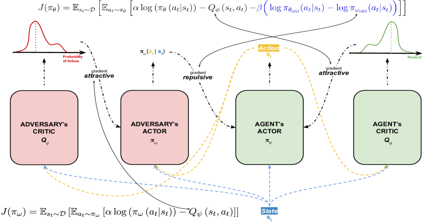
Figure 1: The schematic of the Safe Adversarially guided Actor-Critics ($\mathtt{SAAC}$) algorithm.

As a building block for $\mathtt{SAAC}$, we deploy the recent version of SAC Haarnoja et al. (2018) that uses two soft Q-functions to mitigate positive bias in the policy improvement step in Eq. (3), which was encountered in Hasselt (2010); Fujimoto et al. (2018). In the design of $\mathtt{SAAC}$, we introduce two new ideas: an off-policy deep actor-critic algorithm within the MaxEnt RL framework and a Risk-sensitive Non-zero Sum (RNS) game. $\mathtt{SAAC}$ engages the agent in safer strategies while finding the optimal actions to maximize the expected returns. The role of the adversary is to find a policy that maximizes the probability of breaking the constraints given by the environment. The adversary is trained online with off-policy data given by the agent. We denote the parameter of the adversary policy using $\omega$. For each sequence of transition from the replay buffer, the adversary should find actions that minimize the following loss:

$$J(\pi_{\omega})=\mathbb{E}_{s_{t}\sim\mathcal{D}}\left[\mathbb{E}_{a_{t}\sim\pi_{\omega}}\left[\alpha\log\left(\pi_{\omega}\left(a_{t}|s_{t}\right)\right)-Q_{\psi}\left(s_{t},a_{t}\right)\right]\right].$$

Finally, leveraging the RNS based reduced objective, $\mathtt{SAAC}$ makes the agent’s actor minimize $J(\pi_{\theta})$:

$$J(\pi_{\theta})=\mathbb{E}_{s_{t}\sim\mathcal{D}}\Big{[}\mathbb{E}_{a_{t}\sim\pi_{\theta}}\Big{[}\alpha\log\left(\pi_{\theta}\left(a_{t}|s_{t}\right)\right)-Q_{\phi}\left(s_{t},a_{t}\right){\color[rgb]{0,0,1}-\beta\Big{(}\log\pi_{\theta_{\text{old}}}(a_{t}|s_{t})-\log\pi_{\omega_{\text{old}}}(a_{t}|s_{t})\Big{)}}\Big{]}\Big{]}.$$

In blue is the repulsion term introduced by $\mathtt{SAAC}$. The method alternates between collecting samples from the environment with the current agent’s policy and updating the function approximators, namely the adversary’s critic $Q_{\psi}$, the adversary’s policy $\pi_{\omega}$, the agent’s critic $Q_{\phi}$ and the agent’s policy $\pi_{\theta}$. It performs stochastic gradient descent on corresponding loss functions with batches sampled from the replay buffer. We provide a generic description of $\mathtt{SAAC}$ in Algorithm 1. Now, we provide a few examples of designing the adversary’s critic $Q_{\psi}$ for different safety constraints.

Algorithm 1 $\mathtt{SAAC}$

  Input parameters: $\tau,\lambda_{Q},\lambda_{\pi},\lambda_{\alpha},\lambda_{\beta}$

  Initialize adversary’s and agent’s policies and Q-functions parameters $\omega$, $\psi$, $\theta$ and $\phi$

  Initialize temperature parameters $\alpha$ and $\beta$

  $\mathcal{D}\leftarrow\emptyset$

  for each iteration do

     for each step do

        $a_{t}\sim\pi_{\theta}(a_{t}|s_{t})$

        $s_{t+1}\sim{\cal P}\left(s_{t},a_{t}\right)$

        $\mathcal{D}\leftarrow\mathcal{D}\cup\left\{\left(s_{t},a_{t},r_{t},s_{t+1}\right)\right\}$

     end for

     for each gradient step do

        sample batch $\mathcal{B}$ from $\mathcal{D}$

        $\psi\leftarrow\psi-\lambda_{Q}\hat{\nabla}_{\psi}J_{Q}\left(\psi\right)$  

        $\omega\leftarrow\omega-\lambda_{\pi}\hat{\nabla}_{\omega}J(\pi_{\omega})$

        $\beta\leftarrow\beta-\lambda_{\beta}\hat{\nabla}_{\beta}J(\beta)$

        $\bar{\psi}\leftarrow\tau\psi+(1-\tau)\bar{\psi}$

        $\phi\leftarrow\phi-\lambda_{Q}\hat{\nabla}_{\phi}J_{Q}\left(\phi\right)$    

        $\theta\leftarrow\theta-\lambda_{\pi}\hat{\nabla}_{\theta}J(\pi_{\theta})$

        $\alpha\leftarrow\alpha-\lambda_{\alpha}\hat{\nabla}_{\alpha}J(\alpha)$

        $\bar{\phi}\leftarrow\tau\phi+(1-\tau)\bar{\phi}$

     end for

  end for

$\mathtt{SAAC}$-$\mathtt{Cons}$: Subspace Risk. At every step, the environment signals whether the constraints have been satisfied or not. We construct a reward signal based on this information. This constraint reward, denoted as $r_{c}$, is $1$ if all the constraints have been broken, and $0$ otherwise. $J(Q_{\psi})$ is the soft Bellman residual for the critic responsible with constraint satisfaction:

$$J(Q_{\psi})=\mathbb{E}_{\left(s_{t},a_{t}\right)\sim\mathcal{D}}\Big{[}\frac{1}{2}\Big{(}Q_{\psi}\left(s_{t},a_{t}\right)-\big{(}r_{c}\left(s_{t},a_{t}\right)+\gamma\mathbb{E}_{s_{t+1}\sim\rho}\mathbb{E}_{a_{t}\sim\pi_{\omega}}\left[Q_{\bar{\psi}}\left(s_{t},a_{t}\right)-\alpha\log\pi\left(a_{t}|s_{t}\right)\right]\Big{)}^{2}\Big{]}.$$ (11)

$\mathtt{SAAC}$-$\mathtt{MSD}$: Mean-Standard Deviation (MSD). In this case, we consider optimizing a Mean-Standard Deviation risk Prashanth and Ghavamzadeh (2016), which we estimate using: $Q_{\psi}(s,a)=Q_{\phi}(s,a)+\lambda\sqrt{\mathop{\mbox{$\mathbb{V}$}}\nolimits[Q_{\phi}(s,a)]}.$ $\lambda<0$ is a hyperparameter that dictates the lower $\lambda-\mathrm{SD}$ considered to represent the lower tail. In the experiments, we use $\lambda=-1$. In practice, we approximate the variance $\mathop{\mbox{$\mathbb{V}$}}\nolimits[Q_{\phi}(s,a)]$ using the state-action pairs in the current batch of samples. We refer to the associated method as $\mathtt{SAAC}$-$\mathtt{MSD}$.

$\mathtt{SAAC}$-$\mathtt{CVaR}$: CVaR. Given a state-action pair $(s,a)$, the Q-value distribution is approximated by a set of quantile values at quantile fractions Eriksson et al. (2021). Let $\left\{\tau_{i}\right\}_{i=0,\ldots,N}$ denote a set of quantile fractions, which satisfy $\tau_{0}=0$, $\tau_{N}=1$, $\tau_{i}<\tau_{j}\,\forall i<j$, $\tau_{i}\in[0,1]\,\forall i=0,\ldots,N$, and $\hat{\tau}_{i}=\left(\tau_{i}+\tau_{i+1}\right)/2$. If $Z^{\pi}:\mathcal{S}\times\mathcal{A}\rightarrow\mathcal{Z}$ denotes the soft action-value of policy $\pi$, $Q_{\psi}(s,a)=-\sum_{i=0}^{N-1}\left(\tau_{i+1}-\tau_{i}\right)g^{\prime}\left(\hat{\tau}_{i}\right)Z^{\pi_{\theta}}_{\hat{\tau}_{i}}(s,a;\phi)$ with $g(\tau)=\min\{\tau/\lambda,1\}$, where $\lambda\in(0,1)$. In the experiments, we set $\lambda=0.25$, i.e. we truncate the right tail of the return distribution by dropping 75% of the topmost atoms.

4.3 Automating Adversarial Adjustment

Similar to the solution introduced in Haarnoja et al. (2018), the adversary temperature $\beta$ and the entropy temperature are automatically adjusted. Since the adversary bonus can differ across tasks and during training, a fixed coefficient would be a poor solution. We use $\bar{\mathcal{A}}$ to denote the adversary’s bonus target, which is a hyperparameter in $\mathtt{SAAC}$. By formulating a constrained optimization problem where the KL-divergence between the agent and the adversary is constrained, $\beta$ is learned by gradient descent with respect to:

$$J(\beta)=\mathbb{E}_{s_{t}\sim\mathcal{D}}\left[\log\beta\cdot\left(D_{\mathrm{KL}}\left(\pi_{\theta}(\cdot|s_{t})~{}\middle\|~{}\pi_{\omega}(\cdot|s_{t})\right)-\bar{\mathcal{A}}\right)\right].$$

In addition, the entropy temperature $\alpha$ is also learned by taking a gradient step with respect to the loss:

$$J(\alpha)=\mathbb{E}_{s_{t}\sim\mathcal{D}}\left[\log\alpha\cdot\left(-\log\pi_{\theta}\left(a_{t}|s_{t}\right)-\bar{\mathcal{H}}\right)\right].$$

$\bar{\mathcal{H}}$ is the target entropy: a hyperparameter needed in SAC. We illustrate this in the pseudo-code of SAAC as in Algorithm 1.

5 Experimental Analysis

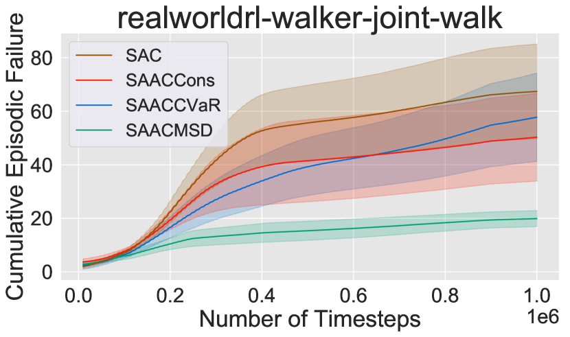
Figure 2: $\mathtt{SAAC}$ variants.

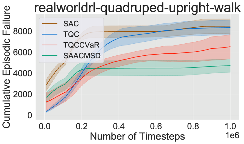
Figure 3: $\mathtt{SAAC}$ vs. baselines.

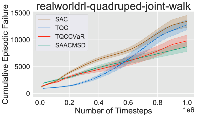
Figure 4: $\mathtt{SAAC}$ vs. baselines.

Experimental Setup. First, we compare some possible variants of our method. Indeed, as presented in Sec. 4.2, the adversary has different quantifications of risk to fulfill the objective of finding actions with high probability of breaking the constraints: $\mathtt{SAAC}$-$\mathtt{Cons}$, $\mathtt{SAAC}$-$\mathtt{CVaR}$, and $\mathtt{SAAC}$-$\mathtt{MSD}$.

Following that, we compare our method with best performing competitors in continuous control problems: SAC Haarnoja et al. (2018) and TQC Kuznetsov et al. (2020). TQC builds on top of C51 Bellemare et al. (2017) and QR-DQN Dabney et al. (2018), and adapt the distributional RL methods for continuous control. Further, they apply truncation for the approximated distributions to control their overestimation and use ensembling on the approximators for additional performance improvement. Finally, we qualitatively compare the behavior of our risk-averse method with that of SAC, using state vectors collected during validation in test environments. Note that for all the experiments (repeated over 9 random seeds), the agents are trained for 1M timesteps and their performance is evaluated at every 1000-th step.

Similar to TQC, we implement $\mathtt{SAAC}$ on top of SAC and choose to automatically tune the adversary temperature $\beta$ (Sec. 4.3) and the entropy temperature $\alpha$. Last but not least, using $\mathtt{SAAC}$ on top of SAC introduces only one hyperparameter: the learning rate for the automatic tuning of $\beta$. All the other hyperparameters are the same as for SAC and are available for consultation in (Haarnoja et al., 2018, Appendix D). For TQC, we employ the same hyperparameters as reported in Kuznetsov et al. (2020).

Description of Environments. To validate the framework of a RNS Game with MaxEnt RL, we conduct a set of experiments in the DM control suite Tassa et al. (2018). More specifically, we use the real-world RL challenge Dulac-Arnold et al. (2020), which introduces a set of real-world inspired challenges. In this paper, we are particularly interested in the tasks, where a set of constraints are imposed on existing control domains. In the following, we give a short description of the tasks and safety constraints used in the experiments, with their respective observation ($\mathcal{S}$) and action ($\mathcal{A}$) dimensions. First, realworldrl-walker-walk ($\mathcal{S}\times\mathcal{A}=18\times 6$) corresponds to the dm-control suite walker task with (a) joint-specific constrains on the joint angles to be within a range and (b) a constrain on the joint velocities to be within a range. Next, realworldrl-quadruped-joint-walk ($\mathcal{S}\times\mathcal{A}=78\times 12$) corresponds to the dm-control suite quadruped task with the same set of constraints as just described. realworldrl-quadruped-upright-walk has a constrain on the quadruped’s torso’s z-axis to be oriented upwards, and realworldrl-quadruped-force-walk limits foot contact forces when touching the ground.

Table 1: Comparison of $\mathtt{SAAC}$ variants.

Method	Efficiency (xSAC)	# Failures $\pm\sigma$
SAC	$\times 1$	$65.88\pm 17.25$
$\mathtt{SAAC}$-$\mathtt{Cons}$	$\times 1.33$	$48.66\pm 15.99$
$\mathtt{SAAC}$-$\mathtt{CVaR}$	$\times 2.02$	$54.39\pm 15.37$
$\mathtt{SAAC}$-$\mathtt{MSD}$	$\mathbf{\times 2.21}$	$\mathbf{19.31\pm 3.02}$

Table 2: In quadruped-upright-walk.

Method	Efficiency (xSAC)	# Failures $\pm\sigma$
SAC	$\times 1$	$8443.93\pm 696.47$
TQC	$\times 0.97$	$8297.63\pm 697.88$
TQC-CVaR	$\times 1.03$	$6298.33\pm 1078.50$
$\mathtt{SAAC}$-$\mathtt{MSD}$	$\mathbf{\times 1.19}$	$\mathbf{4632.80\pm 657.35}$

Table 3: In quadruped-joint-walk.

Method	Efficiency (xSAC)	# Failures $\pm\sigma$
SAC	$\times 1$	$12583.43\pm 997.29$
TQC	$\times 1.07$	$11738.57\pm 995.62$
TQC-CVaR	$\times 1.05$	$9015.82\pm 1011.31$
$\mathtt{SAAC}$-$\mathtt{MSD}$	$\mathbf{\times 1.27}$	$\mathbf{8069.45\pm 803.42}$

5.1 Comparison between Risk Quantifiers of $\mathtt{SAAC}$

First, we compare the different variants of $\mathtt{SAAC}$ allowed by the method’s framework in the realworldrl-walker-walk-returns task. From Table 3 and Fig. 4 (lines are average performances and shaded areas represent one standard deviation) we evaluate how our method affects the performance and risk aversion of agents.

In addition to the rate at which the maximum average return is reached by each of the methods compared to SAC, we compare the cumulative number of failures of the agents (the lower the better). As expected, risk-sensitive agents such as $\mathtt{SAAC}$ decrease the probability of breaking safety constraints. Concurrently, they achieve the maximum average return with much higher sample efficiency, $\mathtt{SAAC}$-$\mathtt{MSD}$ ahead. Henceforth, we use the $\mathtt{SAAC}$-$\mathtt{MSD}$ version of our method to compare with the baselines.

5.2 Comparison of $\mathtt{SAAC}$ to Baselines

Now, we compare the best performing $\mathtt{SAAC}$ variant $\mathtt{SAAC}$-$\mathtt{MSD}$ with SAC Haarnoja et al. (2018), TQC Kuznetsov et al. (2020) and TQC-CVaR, i.e. an extension of TQC with 16% of the topmost atoms dropped (cf. Table 6 in (Kuznetsov et al., 2020, Appendix B)) of all Q-function atoms. In Table 3 and Fig. 4, we evaluate $\mathtt{SAAC}$-$\mathtt{MSD}$ in realworldrl-quadruped-upright-walk. In Table 3 and Fig. 4, we report the results for realworldrl-quadruped-joint-walk.

Table 3 shows that $\mathtt{SAAC}$-$\mathtt{MSD}$ performs better than all other baselines both in terms of final performance and in terms of finding risk-averse policies. Moreover, although TQC-CVaR exhibits fewer number of failures over the course of learning, it performs slightly worse than its non-truncated counterpart TQC. Table 3 confirms the advantage of using $\mathtt{SAAC}$-$\mathtt{MSD}$ as a risk-averse MaxEnt RL method over the baselines: overall using $\mathtt{SAAC}$ allows the agents to achieve faster convergence using safer policies during training. Interestingly, TQC achieves the maximum score of the task a bit later than the SAC agent. Nevertheless, TQC-CVaR, its CVaR variant, opens the door for better sample efficiency score with much safer policies.

5.3 Visualization of Safer State Space Visitation

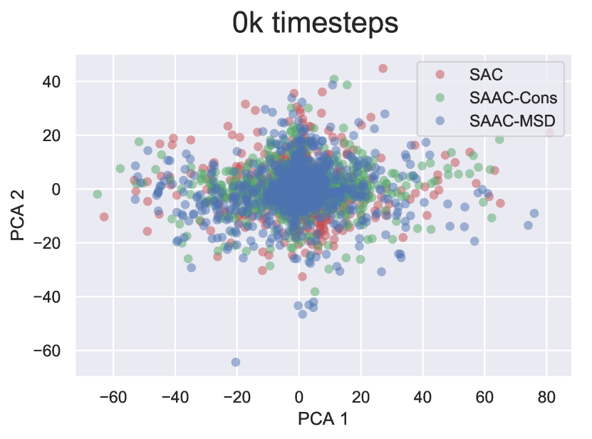
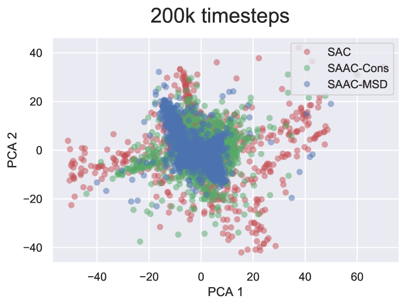
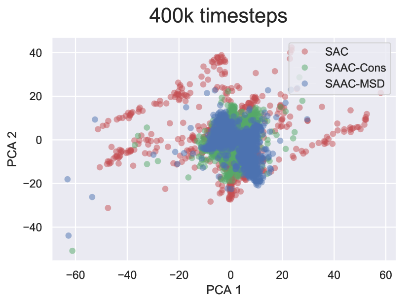
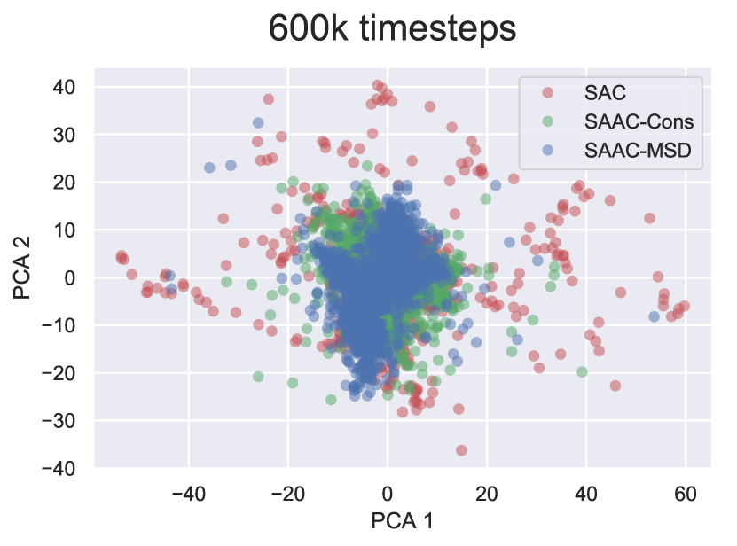
Figure 5: Visualization of visited state space projection at different stages of learning in the realworldrl-walker-walk task.

In this experiment, we choose SAC, $\mathtt{SAAC}$-$\mathtt{Cons}$ and $\mathtt{SAAC}$-$\mathtt{MSD}$ to train a relatively wide spectrum of agents using the same experimental protocol as in Sec. 5.2., and on the realworldrl-walker-walk task. We collect samples of states visited during the evaluation phase in a test environment at different stages of the training. The state vectors are projected from a 18D space to a 2D space using PCA. We present the results in Fig. 5. At the beginning of training, there is no clear distinction in terms of explored state regions, as the learning has not begun yet. On the contrary, during the 200k-600k timesteps, there is a significant difference in terms of state space visitation. In resonance with the cumulative number of failures shown in Fig. 4, the results suggest that SAC engages in actions leading to more unsafe states. Conversely, $\mathtt{SAAC}$ seems to successfully constraint the agents to safe regions.

6 Discussion and Future Work

In this paper, we address the problem of risk-sensitive RL under safety constraints and coherent risk measures. We propose that maximizing the value function under risk or safety constraints is equivalent to playing a risk-sensitive non-zero sum (RNS) game. In the RNS game, an adversary tries to maximize the risk of a decision trajectory while the agent tries to maximize a weighted sum of its value function given the adversary’s feedback. Specifically, under the MaxEnt RL framework, this RNS game reduces to deploying two soft-actor critics for the agent and the adversary while accounting for a repulsion term between their policies. This allows us to formulate a duelling SAC-based algorithm, called $\mathtt{SAAC}$. We instantiate our method for subspace, mean-standard deviation, and CVaR constraints, and also experimentally test it on various continuous control tasks. Our algorithm leads to better risk-sensitive performance than SAC and the risk-sensitive distributional RL baselines in all these environments. In future work, further study on leveraging the flexibility of $\mathtt{SAAC}$ to incorporate more safety constraints is anticipated.

References

- Ahmed et al. (2019) Zafarali Ahmed, Nicolas Le Roux, Mohammad Norouzi, and Dale Schuurmans. Understanding the impact of entropy on policy optimization. In International Conference on Machine Learning, pages 151–160. PMLR, 2019.
- Altman (1999) Eitan Altman. Constrained Markov decision processes, volume 7. CRC Press, 1999.
- Artzner et al. (1999) Philippe Artzner, Freddy Delbaen, Jean-Marc Eber, and David Heath. Coherent measures of risk. Mathematical finance, 9(3):203–228, 1999.
- Bellemare et al. (2017) Marc G Bellemare, Will Dabney, and Rémi Munos. A distributional perspective on reinforcement learning. In International Conference on Machine Learning, pages 449–458. PMLR, 2017.
- Berkenkamp et al. (2016) Felix Berkenkamp, Riccardo Moriconi, Angela P. Schoellig, and Andreas Krause. Safe learning of regions of attraction for uncertain, nonlinear systems with Gaussian processes. In IEEE CDC, pages 4661–4666, 2016.
- Chen et al. (2005) Xinjia Chen, Jorge L Aravena, and Kemin Zhou. Risk analysis in robust control-making the case for probabilistic robust control. In Proceedings of the 2005, American Control Conference, 2005., pages 1533–1538. IEEE, 2005.
- Chow and Ghavamzadeh (2014) Y. Chow and M. Ghavamzadeh. Algorithms for CVaR optimization in MDPs. In Advances in neural information processing systems, pages 3509–3517, 2014.
- Chow et al. (2015) Y. Chow, A. Tamar, S. Mannor, and M. Pavone. Risk-sensitive and robust decision-making: a cvar optimization approach. In Advances in Neural Information Processing Systems, pages 1522–1530, 2015.
- Chow et al. (2017) Yinlam Chow, Mohammad Ghavamzadeh, Lucas Janson, and Marco Pavone. Risk-constrained reinforcement learning with percentile risk criteria. The Journal of Machine Learning Research, 18(1):6070–6120, 2017.
- Coraluppi and Marcus (1999) Stefano P Coraluppi and Steven I Marcus. Risk-sensitive and minimax control of discrete-time, finite-state Markov decision processes. Automatica, 35(2):301–309, 1999.
- Dabney et al. (2018) Will Dabney, Mark Rowland, Marc Bellemare, and Rémi Munos. Distributional reinforcement learning with quantile regression. In Proceedings of the AAAI Conference on Artificial Intelligence, 2018.
- Degrave et al. (2019) Jonas Degrave, Michiel Hermans, Joni Dambre, et al. A differentiable physics engine for deep learning in robotics. Frontiers in neurorobotics, 13:6, 2019.
- Dulac-Arnold et al. (2020) Gabriel Dulac-Arnold, Nir Levine, Daniel J Mankowitz, Jerry Li, Cosmin Paduraru, Sven Gowal, and Todd Hester. An empirical investigation of the challenges of real-world reinforcement learning. arXiv preprint arXiv:2003.11881, 2020.
- Eriksson et al. (2021) Hannes Eriksson, Debabrota Basu, Mina Alibeigi, and Christos Dimitrakakis. SENTINEL: Taming uncertainty with ensemble-based distributional reinforcement learning. arXiv preprint arXiv:2102.11075, 2021.
- Eysenbach and Levine (2019) Benjamin Eysenbach and Sergey Levine. If MaxEnt RL is the answer, what is the question? arXiv preprint arXiv:1910.01913, 2019.
- Eysenbach and Levine (2021) Benjamin Eysenbach and Sergey Levine. Maximum entropy RL (provably) solves some robust RL problems. arXiv preprint arXiv:2103.06257, 2021.
- Fujimoto et al. (2018) Scott Fujimoto, Herke Hoof, and David Meger. Addressing function approximation error in actor-critic methods. In International Conference on Machine Learning, pages 1587–1596. PMLR, 2018.
- Garcıa and Fernández (2015) Javier Garcıa and Fernando Fernández. A comprehensive survey on safe reinforcement learning. Journal of Machine Learning Research, 16(1):1437–1480, 2015.
- Geibel and Wysotzki (2005) Peter Geibel and Fritz Wysotzki. Risk-sensitive reinforcement learning applied to control under constraints. Journal of Artificial Intelligence Research, 24:81–108, 2005.
- Gibney (2016) Elizabeth Gibney. Google AI algorithm masters ancient game of Go. Nature News, 529(7587):445, 2016.
- Haarnoja et al. (2018) Tuomas Haarnoja, Aurick Zhou, Kristian Hartikainen, George Tucker, Sehoon Ha, Jie Tan, Vikash Kumar, Henry Zhu, Abhishek Gupta, Pieter Abbeel, and Sergey Levine. Soft actor-critic algorithms and applications. arXiv preprint arXiv:1812.05905, 2018.
- Hasselt (2010) Hado Hasselt. Double Q-learning. Advances in neural information processing systems, 23:2613–2621, 2010.
- Heger (1994) Matthias Heger. Consideration of risk in reinforcement learning. In Machine Learning Proceedings 1994, pages 105–111. Elsevier, 1994.
- Howard and Matheson (1972) Ronald A Howard and James E Matheson. Risk-sensitive Markov decision processes. Management science, 18(7):356–369, 1972.
- Koller et al. (2018) Torsten Koller, Felix Berkenkamp, Matteo Turchetta, and Andreas Krause. Learning-based model predictive control for safe exploration. In 2018 IEEE Conference on Decision and Control (CDC), pages 6059–6066. IEEE, 2018.
- Kuznetsov et al. (2020) Arsenii Kuznetsov, Pavel Shvechikov, Alexander Grishin, and Dmitry Vetrov. Controlling overestimation bias with truncated mixture of continuous distributional quantile critics. In ICML, pages 5556–5566. PMLR, 2020.
- Lillicrap et al. (2015) Timothy P Lillicrap, Jonathan J Hunt, Alexander Pritzel, Nicolas Heess, Tom Erez, Yuval Tassa, David Silver, and Daan Wierstra. Continuous control with deep reinforcement learning. arXiv preprint arXiv:1509.02971, 2015.
- Lim and Shanthikumar (2007) Andrew EB Lim and J George Shanthikumar. Relative entropy, exponential utility, and robust dynamic pricing. Operations Research, 55(2):198–214, 2007.
- Marcus et al. (1997) Steven I Marcus, Emmanual Fernández-Gaucherand, Daniel Hernández-Hernandez, Stefano Coraluppi, and Pedram Fard. Risk sensitive markov decision processes. In Systems and control in the twenty-first century, pages 263–279. Springer, 1997.
- Mnih et al. (2015) Volodymyr Mnih, Koray Kavukcuoglu, David Silver, Andrei A Rusu, Joel Veness, Marc G Bellemare, Alex Graves, Martin Riedmiller, Andreas K Fidjeland, Georg Ostrovski, et al. Human-level control through deep reinforcement learning. Nature, 518(7540):529–533, 2015.
- Neu et al. (2017) Gergely Neu, Anders Jonsson, and Vicenç Gómez. A unified view of entropy-regularized Markov decision processes. arXiv preprint arXiv:1705.07798, 2017.
- Pan et al. (2017) Xinlei Pan, Yurong You, Ziyan Wang, and Cewu Lu. Virtual to real reinforcement learning for autonomous driving. arXiv preprint arXiv:1704.03952, 2017.
- Pinto et al. (2017) Lerrel Pinto, James Davidson, Rahul Sukthankar, and Abhinav Gupta. Robust adversarial reinforcement learning. In International Conference on Machine Learning, pages 2817–2826. PMLR, 2017.
- Prashanth and Fu (2018) A Prashanth and Michael Fu. Risk-sensitive reinforcement learning: A constrained optimization viewpoint. arXiv e-prints, pages arXiv–1810, 2018.
- Prashanth and Ghavamzadeh (2016) LA Prashanth and Mohammad Ghavamzadeh. Variance-constrained actor-critic algorithms for discounted and average reward MDPs. Machine Learning, 105(3):367–417, 2016.
- Puterman (2014) Martin L Puterman. Markov decision processes: discrete stochastic dynamic programming. John Wiley & Sons, 2014.
- Ray et al. (2019) Alex Ray, Joshua Achiam, and Dario Amodei. Benchmarking safe exploration in deep reinforcement learning. arXiv preprint arXiv:1910.01708, 2019.
- Rockafellar et al. (2000) R Tyrrell Rockafellar, Stanislav Uryasev, et al. Optimization of conditional value-at-risk. Journal of risk, 2:21–42, 2000.
- Sorin (1986) S Sorin. Asymptotic properties of a non-zero sum stochastic game. International Journal of Game Theory, 15(2):101–107, 1986.
- Sutton and Barto (2018) Richard S Sutton and Andrew G Barto. Reinforcement learning: An introduction. MIT press, 2018.
- Szegö (2004) Giorgio P Szegö. Risk measures for the 21st century, volume 1. Wiley New York, 2004.
- Tassa et al. (2018) Yuval Tassa, Yotam Doron, Alistair Muldal, Tom Erez, Yazhe Li, Diego de Las Casas, David Budden, Abbas Abdolmaleki, Josh Merel, Andrew Lefrancq, et al. Deepmind control suite. arXiv preprint arXiv:1801.00690, 2018.
- Thananjeyan et al. (2021) Brijen Thananjeyan, Ashwin Balakrishna, Suraj Nair, Michael Luo, Krishnan Srinivasan, Minho Hwang, Joseph E Gonzalez, Julian Ibarz, Chelsea Finn, and Ken Goldberg. Recovery RL: Safe reinforcement learning with learned recovery zones. IEEE Robotics and Automation Letters, 6(3):4915–4922, 2021.
- Todorov (2007) Emanuel Todorov. Linearly-solvable Markov decision problems. In Advances in neural information processing systems, pages 1369–1376, 2007.
- Toussaint (2009) Marc Toussaint. Robot trajectory optimization using approximate inference. In Proceedings of the 26th annual international conference on machine learning, pages 1049–1056, 2009.
- Wachi and Sui (2020) Akifumi Wachi and Yanan Sui. Safe reinforcement learning in constrained Markov decision processes. In International Conference on Machine Learning, pages 9797–9806. PMLR, 2020.
- Williams and Peng (1991) Ronald J Williams and Jing Peng. Function optimization using connectionist reinforcement learning algorithms. Connection Science, 3(3):241–268, 1991.
- Wu (1983) C. F. Jeff Wu. On the Convergence Properties of the EM Algorithm. The Annals of Statistics, 11(1):95 – 103, 1983.