∎
22email: jfcai@ust.hk 33institutetext: M. Huang 44institutetext: School of Mathematical Sciences, Beihang University, Beijing, 100191, China
44email: menghuang@buaa.edu.cn 55institutetext: D. Li 66institutetext: SUSTech International Center for Mathematics and Department of Mathematics, Southern University of Science and Technology, Shenzhen, China
66email: lid@sustech.edu.cn 77institutetext: Y. Wang 88institutetext: Department of Mathematics, The Hong Kong University of Science and Technology, Hong Kong, China
88email: yangwang@ust.hk
Nearly optimal bounds for the global geometric landscape of phase retrieval ††thanks: J. F. Cai was supported in part by Hong Kong Research Grant Council grants 16309518, 16309219, 16310620, 16306821. Y. Wang was supported in part by the Hong Kong Research Grant Council grants 16306415 and 16308518.
Abstract
The phase retrieval problem is concerned with recovering an unknown signal from a set of magnitude-only measurements . A natural least squares formulation can be used to solve this problem efficiently even with random initialization, despite its non-convexity of the loss function. One way to explain this surprising phenomenon is the benign geometric landscape: (1) all local minimizers are global; and (2) the objective function has a negative curvature around each saddle point and local maximizer. In this paper, we show that Gaussian random measurements are sufficient to guarantee the loss function of a commonly used estimator has such benign geometric landscape with high probability. This is a step toward answering the open problem given by Sun-Qu-Wright Sun18 , in which the authors suggest that or even is enough to guarantee the favorable geometric property.
Keywords:
Phase retrieval Geometric landscape Nonconvex optimizationMSC:
94A12 65K10 49K451 Introduction
1.1 Background
In a prototypical phase retrieval problem, one is interested in how to recover an unknown signal from a series of magnitude-only measurements
| (1) |
where are given vectors and is the number of measurements. This problem is of fundamental importance in numerous areas of physics and engineering such as X-ray crystallography harrison1993phase ; millane1990phase , microscopy miao2008extending , astronomy fienup1987phase , coherent diffractive imaging shechtman2015phase ; Gerchberg1972 and optics walther1963question etc, where the optical detectors can only record the magnitude of signals while losing the phase information. Despite its simple mathematical formulation, it has been shown that reconstructing a finite-dimensional discrete signal from the magnitude of its Fourier transform is generally an NP-complete problem Sahinoglou .
Due to the practical ubiquity of the phase retrieval problem, many algorithms have been designed for this problem. For example, based on the technique “matrix-lifting”, the phase retrieval problem can be recast as a low rank matrix recovery problem. By using convex relaxation one can show that the matrix recovery problem under suitable conditions is equivalent to a convex optimization problem phaselift ; Phaseliftn ; Waldspurger2015 . However, since the matrix-lifting technique involves semidefinite program for matrices, the computational cost is prohibitive for large scale problems. In contrast, many non-convex algorithms bypass the lifting step and operate directly on the lower-dimensional ambient space, making them much more computationally efficient. Early non-convex algorithms were mostly based on the technique of alternating projections, e.g. Gerchberg-Saxton Gerchberg1972 and Fineup ER3 . The main drawback, however, is the lack of theoretical guarantee. Later Netrapalli et al AltMin proposed the AltMinPhase algorithm based on a technique known as spectral initialization. They proved that the algorithm linearly converges to the true solution with resampling Gaussian random measurements. This work led further to several other non-convex algorithms based on spectral initialization. A common thread is first choosing a good initial guess through spectral initialization, and then solving an optimization model through gradient descent, such as WF ; TWF ; Gaoxu ; TAF ; RWF ; huangwang ; tan2019phase . We refer the reader to survey papers shechtman2015phase ; Chinonconvex ; jaganathan2016phase for accounts of recent developments in the theory, algorithms and applications of phase retrieval.
1.2 Prior arts and motivation
As stated earlier, producing a good initial guess using carefully-designed initialization seems to be a prerequisite for prototypical non-convex algorithms to succeed with good theoretical guarantee. A natural and fundamental question is:
Is it possible for non-convex algorithms to achieve successful recovery with a random initialization ?
Recently, Ju Sun et al. carried out a deep study of the global geometric structure of the loss function:
| (2) |
where are measurements given in (1). They proved that the loss function does not possess any spurious local minima under Gaussian random measurements. More specifically, it was shown in Sun18 that all minimizers of coincide with the target signal up to a global phase, and has a negative directional curvature around each saddle point. Thanks to this benign geometric landscape any algorithm which can avoid strict saddle points converges to the true solution with high probability. A trust-region method was employed in Sun18 to find the global minimizers with random initialization. The results in Sun18 require samples to guarantee the favorable geometric property and efficient recovery. On the other hand, based on ample numerical evidences, the authors of Sun18 conjectured that the optimal sampling complexity could be or even to guarantee the benign landscape of the loss function (cf. p. 1160 therein).
In this paper, we focus on this conjecture and prove that the loss function possesses the favorable geometric property, as long as the measurement number , by some sophisticated analysis. In other words, we prove that (1) all local minimizers of the loss function are global; and (2) the objective function has a negative curvature around each saddle point and local maximizer. This is a step toward proving the open problem.
We shall emphasize that if allowing some modifications to the loss function , the sampling complexity can be reduced to the optimal bound 2020b ; 2020c ; cai2019 . In cai2019 the authors show that a combination of the loss function (2) with a judiciously chosen activation function also has the benign geometry structure under Gaussian random measurements. Furthermore, in our recent work 2020a , we consider another new smoothed amplitude flow estimator which is based on a piece-wise smooth modification to the loss function
| (3) |
and we could also prove that the loss function (3) after some modifications has a benign geometric landscape under the optimal sampling threshold .
The emerging concept of a benign geometric landscape has also recently been explored in many other applications of signal processing and machine learning, e.g. matrix sensing bhojanapalli2016global ; park2016non , tensor decomposition ge2016matrix , dictionary learningsun2016complete and matrix completion ge2015escaping . For general optimization problems there exist a plethora of loss functions with well-behaved geometric landscapes such that all local optima are also global optima and each saddle point has a negative direction curvature in its vincinity. Correspondingly several techniques have been developed to guarantee that the standard gradient based optimization algorithms can escape such saddle points efficiently, see e.g. jin2017escape ; du2017gradient ; jin2017accelerated .
1.3 Our contributions
In this paper, we focus on the open problem: what is the optimal sampling complexity to guarantee the loss function given in (2) has favorable geometric landscape? We develop several new techniques and prove that Gaussian random measurements are enough. While we can not prove the optimality of this bound, it is an improvement over the result of given in Sun18 . The main result of our paper is the following theorem.
Theorem 1.1
Assume that are i.i.d. standard Gaussian random vectors and is a fixed vector. There exist positive absolute constants , and , such that if , then with probability at least the loss function defined by (2) has no spurious local minimizers. In other words, the only local minimizer is up to a global phase and all saddle points are strict, i.e., each saddle point has a neighborhood where the function has negative directional curvature. Moreover, the loss function is strongly convex in a neighborhood of , and the point is a local maximum point where the Hessian is strictly negative-definite.
Remark 1
For simplicity we consider here only the real-valued case and will investigate the complex-valued case elsewhere. In Theorem 1.1 the probability bound can be refined.
Remark 2
Another interesting issue is to show the measurements are non-adaptive, i.e., a single realization of measurement vectors can be used to reconstruct all . However we shall not dwell on this refinement here for simplicity.
1.4 Notations
Throughout the paper, we write if and . We use to denote the usual characteristic function. For example if and if . For any quantity , we shall write if for some constant . We write if for some universal constant . We shall write if where the constant will be sufficiently small. We use to denote where is a universal constant. In this paper, we use and the subscript (superscript) form of them to denote universal constants whose values vary with the context.
1.5 Organization
The rest of the papers are organized as follows. In Section 2, we divide the whole space into several regions and investigate the geometric property of on each region. In Section 3, we present the detailed justification for the technical lemmas given in Section 2. Finally, the appendix collects some auxiliary estimates needed in the proof.
2 Proof of the main result
In the rest of this section we shall carry out the proof of Theorem 1.1 in several steps. More specifically, we decompose into several regions (not necessarily non-overlapping), on each of which has certain property that will allow us to show that with high probability has no local minimizers other than . Furthermore, we show is strongly convex in a neighborhood of .
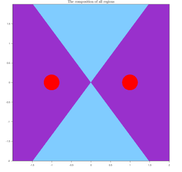
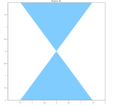
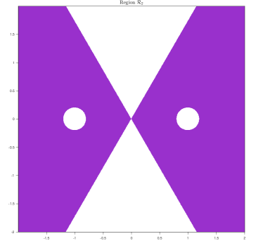
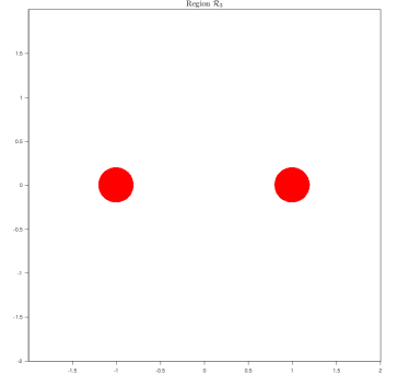
Without loss of generality, we assume . Denote . Then we can decompose into three regions as shown below.
-
•
,
-
•
,
-
•
,
where is arbitrary small positive constant and is a universal constant. Figure 1 visualizes the partitioning regions described above and gives the idea of how they cover the whole space.
The properties of over these regions are summarized in the following three lemmas.
Lemma 1
For any there exists a constant such that with probability at least it holds: any critical point obeys
provided . Here, and are positive constants depending only on , and is a universal constant.
Lemma 2
Assume that . Then with probability at least there is no critical point in the region . Here, and are constants depending only on .
Lemma 3
Assume that . There exists a constant such that with probability at least we have for all and unit vectors . In other words, is strongly convex in . Here, and are constants depending only on .
The proofs of the above lemmas are given in Section 3. Lemma 2 guarantee the gradient of does not vanish in . Thus the critical points of can only occur in and . However, Lemma 1 shows that at any critical point in , has a negative directional curvature. Finally, Lemma 3 implies that is strongly convex in . Recognizing that and , thus is the local minimizer. Putting it all together, we can establish Theorem 1.1 as shown below.
Proof of Theorem 1.1 For any being a possible critical point and satisfying , Lemma 1 shows that has a negative directional curvature. For any satisfying and , Lemma 2 demonstrates that the gradient . Finally, when is very close to the target solutions , is strongly convex and are the global solutions. ∎
3 Proofs of technical results in Section 2
The basic idea of the proof is to show for each critical point except there is a negative curvature direction.
3.1 Proof of Lemma 1
Proof For any , denote
| (4) |
Recall the function
| (5) |
Through a simple calculation, the Hessian of the function along the direction can be denote by
We first show that is a local maximum. Indeed, by Corollary 2 in the appendix, if then it holds with probability at least that
Here, and are universal positive constants. This means that with high probability the Hessian is strictly negative definite.
Next, we consider the case where and prove the loss function (5) has a negative curvature at each critical point in the regime . Through a simple calculation, we have
If at some we have a critical point, then
where is defined by (4). By Lemma 11, if then it holds with probability at least that . Here, is a universal constant. Consequently, if at some we have a critical point, then it holds
| (6) |
On the other hand, the Hessian at this point along the direction is
Using the equation (6), we obtain
| (7) |
We claim that for any , when , with probability at least , the following holds:
| (8) |
where are constants depending only on and is a universal constant. On the other hand, by Lemma 11, when , with probability at least it holds
| (9) |
Putting (8) and (9) into (7), we obtain that for , with probability at least , it holds
Since the term is the sum of nonnegative random variables, the deviation below its expectation is bounded and the lower-tail is well-behaved. More concretely, by Lemma 11, if then with probability at least we have
It immediately gives
for some constant by taking to be sufficiently small (depending on ), provided . Here, is an absolute constant. This means the Hessian matrix has a negative curvature along the direction , which proves the lemma.
Finally, it remains to prove the claim (8). Due to the heavy tail of fourth powers of Gaussian random variables, to prove the result with sampling complexity , we need to decompose it into several parts by a Lipschitz continuous truncated function. To do this, take , for all , for and for . We can write
Next, we give upper bounds for the terms and . Thanks to the smooth cut-off, can be well bounded. By Lemma 12, for any , there exist constants depending on such that if then with probability at least it holds that
Moreover, note that
Since , it then follows from Lemma 6 that for sufficiently large (depending only on ) we have
which means
For the terms and , when is sufficiently large depending only on , applying Lemma 10 gives
with probability at least provided . Here, and are universal positive constants. Thus for and , by Cauchy-Schwarz inequality, we have
Collecting the above estimators together gives that when , with probability at least , it holds
which completes the proof of claim (8). ∎
3.2 Proof of Lemma 2
Proof Without loss of generality we can assume . For any , denote
| (10) |
Recognize that
At any potential critical point , we should have . Thus gives
Similarly, according to we have
Combining the above two equations leads to the following fundamental relation for any critical point :
| (11) |
Observe that
where . By Corollary 3, for any , if then with probability at least it holds
| (12) |
For the convenience, we denote
We claim that for any , if then with probability at least the following holds:
| (13) |
and
| (14) |
Putting (12), (13) and (14) into (11), we immediately have
| (15) |
with probability at least , provided . By Lemma 11, for with probability at least it holds that
| (16) |
In particular, we have . Then we can simplify (15) as
| (17) |
Note that , which means . On the other hand, recall that . By taking to be sufficiently small, it then follows from (17) that must be sufficiently close to . It implies that for any , if then with probability at least it holds
| (18) |
Furthermore, it follows from the equality in (17) that
Combining with (16) gives the desired two-way bound for that
On the other hand, it follows from (13) that if then with probability at least it holds
This immediately means that the term also has the desired two-way bounds
Finally if is a critical point, then by (6), we have
Since we have already shown that and are well-bounded, it then follows that
| (19) |
Combining (18) and (19), we obtain that if is a critical point then it holds
by taking . This contradicts to the condition that for all . Thus, the loss function has no critical point on . We arrive at the conclusion.
Finally, it remains to prove the claims (13) and (14). Let be such that for all , for and for . Then we can write
where
Through a simple calculation, we have
Using the same procedure as the claim (8), it is easy to derive from Lemma 12, Lemma 6 and Lemma 15 that for any if then with probability at least it holds
and
To deal with the error terms, observe that
Using the Lemma 15 again, we obtain that when , with probability at least it holds
3.3 Proof of Lemma 3
This section goes in the direction of showing the loss function is strongly convex in a neighborhood of , as demonstrated in Lemma 3.
Proof Recall that along any direction ,
To prove the lemma, it suffices to give a lower bound for the first term and an upper bound for the second term. Indeed, for the second term , by Lemma 17, for any if then with probability at least it holds
Here, we use the fact that . For the first term , denote where . Take such that for all , for and for . It is easy to see
By Lemma 12, for any when with probability at least , it holds that
On the other hand, it follows from Lemma 6 that there exists sufficiently large (depending only on ) such that
Collecting the above estimators, we have that when , with probability at least , it holds
| (20) | |||||
for all . Here, we use the fact that in the first inequality. Recall that . It means
| (21) |
Without loss of generality we assume . It then follows from (21) that
Putting it into (20), we have
Note that . By taking sufficiently small we arrive at the conclusion. ∎
4 Appendix: Preliminaries and supporting lemmas
In this section we shall adopt the following convention.
-
•
For a random variable , we shall sometimes use “mean” to denote . This notation is particularly handy when is given by a sum of random variables involving various truncations and modifications.
-
•
For a random variable , the sub-exponential orlicz norm is defined as
In particular . Similarly the sub-gaussian orlicz norm is
-
•
We denote as a sequence of i.i.d. random vectors which are copies of a standard Gaussian random vector satisfying .
Lemma 4 (Hoeffding’s inequality, Vershynin2018 )
Let , be independent, mean zero, sub-gaussian random variables. Let . Then for every , we have
where .
Lemma 5 (Bernstein’s inequality, Vershynin2018 )
Let , be independent, mean zero, sub-exponential random variables. Let . Then for every , we have
where .
Lemma 6
For any , there exists , such that for any , we have
where , .
Proof Since are i.i.d., it suffices to prove the statement for a single random vector . Noting that and , we have
if is sufficiently large. Note that one can easily quantify in terms of . However we shall not dwell on this here. ∎
Lemma 7
Let . For any , if then
In particular, for , with probability at least , we have
Here, and are universal positive constants.
Proof We briefly sketch the standard proof here for the sake of completeness. By using a -net on with and , we have
Now for a pair of fixed , , since , by using Lemma 5, we have for any ,
For any , taking and , we have
provided . Here, and are universal positive constants. ∎
Lemma 8
Suppose is a locally Lipschitz continuous function such that
Assume that for a standard Gaussian random variable . For any , if , then with probability at least , it holds
Here, and are universal positive constants.
Proof Introduce a -net on with . Observe that by Lemma 5, for any , it holds
By Lemma 7, we have for with probability at least , it holds that
Thus with probability at least and uniformly for , , we have
Now we take and . It follows that for with probability at least
the desired inequality holds uniformly for all . ∎
Corollary 1
Let . Assume . There exists such that for any , with probability at least , it holds
Proof We choose such that for , for , and for all . Clearly then
We can then apply Lemma 8 with . Note that (below is a standard normal random variable)
if . ∎
Lemma 9
Let : be independent random variables with
Then for any ,
Proof
Without loss of generality we can assume has zero mean. The result then follows from Markov’s inequality and the observation
Lemma 10
Let . Assume . There exists such that for any , with probability at least , we have
Here, and are universal positive constants.
Proof
Lemma 11
For any , there exist constants only depending on such that if , then the following holds with probability at least :
Proof
Let be such that for all , for and for . Then for any ,
We first take sufficiently large (depending only on ) such that
where . Then by using Lemma 8, we have for ,
The desired result then easily follows.
Lemma 12
Suppose are Lipschitz continuous functions such that
where is a constant. Assume that for a standard Gaussian random variable . For any , there exist constant only depending on and universal constant such that if , then with probability at least , we have
Proof
Introduce a -net on with . By Lemma 5, for any , we have
where is a universal constant. Next by Lemma 7 and 8, if then with probability at least , it holds
where are universal positive constants. Consequently, for any , there exist such that , , and then
Now set and . The desired conclusion then follows with probability at least
provided . Here, is a positive universal constant and is a positive constant only depending on .
Corollary 2
If , then with probability at least , we have
where and are absolute positive constants.
Proof
Step 1. Write , where , and is such that . Let and denote , . Clearly , and , are independent. Now let . We have
where is an absolute constant, and is taken to be a sufficiently large absolute constant.
Step 2. Let be such that for and for . Clearly if , then with probability at least , we have
and thus
Lemma 13
Let be a Lipschitz continuous function such that
Define the set
Suppose satisfies . For any , if , then with probability at least , we have
Proof
First it is easy to check that . By Lemma 4, for each , we have
Now let and introduce a -net on the set . Note that the set can be identified as a unit ball in . We have . Thus
By Lemma 7, if , then with probability at least , we have
Now if , with , then with probability at least , we have
where , are absolute constants. On the other hand
It follows that for some absolute constant ,
Now set . The desired conclusion then follows with probability at least
provided , where is an absolute constant.
Lemma 14
Let be a Lipschitz continuous function such that
Let be such that
Define
Then for any , there exist , , such that if , then the following holds with probability at least :
Proof
Step 1. Set . Denote
By Lemma 9, we have
Then with probability at least , we have
where is some absolute constant.
Step 2. Denote . An important observation is that and are independent. Note that for we have . Thus for every with the property , we have the following as a consequence of Lemma 13: For any , if , then with probability at least , we have
Step 3. By using the results from Step 1 and Step 2, with probability at least , we have
Now note that . By Lemma 9, we have
Choosing where is a sufficiently large absolute constant such that
then yields the result.
Corollary 3
For any , there exist , , such that if , then the following holds with probability at least :
Proof
We decompose , where . The result then easily follows from Lemma 14.
Lemma 15
For any , there exists , , , such that if , then the following hold with probability at least : For any , we have
Proof
We only sketch the proof. Write , where . For the first inequality, note that (observe )
For the first term one can use Lemma 9. For the second term one can use Lemma 14.
Now for the second inequality, we write
For , by using the estimates already obtained in the beginning part of this proof, it is clear that we can take sufficiently large such that . After is fixed, we return to the estimate of . Note that we can work with a smoothed cut-off function instead of the strict cut-off. The result then follows from Lemma 12 by taking sufficiently large.
Lemma 16
Define . Suppose satisfies and . For any , if , then with probability at least , it holds that
Proof
Let and introduce a -net on the set . Note that the set can be identified as a unit ball in . We have . Introduce the operator
We have
By Lemma 5, for each , we have
Thus
Taking and then yields the result.
Corollary 4
Suppose , are locally Lipschitz continuous functions such that
Define . Suppose satisfies and . For any , there exist a constant , such that if , then with probability at least , it holds that
Proof
Let and introduce a -net with on the set . As we shall see momentarily, we will need to take . By Lemma 5, we have
Now for any , with , , we have
where is an absolute constant. Now introduce the operator
By Lemma 16, with probability at least , we have
Thus with the same probability, we have
where is another absolute constant. It is also not difficult to control the differences in expectation, i.e. for some absolute constant ,
Now take and the desired result clearly follows by taking .
Lemma 17
For any , there are constants , , such that if , then with probability at least , it holds
Proof
Write , where . Then
Clearly the first two terms can be easily handled by Lemma 9 and Lemma 14 respectively. For these terms we actually only need . To handle the last term we need . The main observation is that and are independent. Write and observe that with probability at least , we have
For , by using Lemma 16, it holds with probability at least that
By Lemma 9, we have with probability ,
The desired result then easily follows.
References
- (1) Bhojanapalli, S., Behnam, N., Srebro, N.: Global optimality of local search for low rank matrix recovery. In: Advances in Neural Information Processing Systems, pp. 3873–3881 (2016)
- (2) Cai, J. F., Huang, M., Li, D., Wang, Y.: Solving phase retrieval with random initial guess is nearly as good as by spectral initialization. Appl. Comput. Harmon. Anal. vol. 58, pp. 60–84 (2022)
- (3) Cai, J. F., Huang, M., Li, D., Wang, Y.: The global landscape of phase retrieval I: Perturbed Amplitude Models. Ann. Appl. Math. 37(4), 437–512 (2021)
- (4) Cai, J. F., Huang, M., Li, D., Wang, Y.: The global landscape of phase retrieval II: Quotient Intensity Models. Ann. Appl. Math. 38 (1), 62–114 (2022)
- (5) Candès, E. J., Li, X.: Solving quadratic equations via PhaseLift when there are about as many equations as unknowns. Found. Comut. Math. 14(5), 1017–1026 (2014)
- (6) Candès, E. J. , Li, X., Soltanolkotabi, M.: Phase retrieval via Wirtinger flow: Theory and algorithms. IEEE Trans. Inf. Theory. 61(4), 1985–2007 (2015)
- (7) Candès, E. J., Strohmer, T., Voroninski, V.: Phaselift: Exact and stable signal recovery from magnitude measurements via convex programming. Commun. Pure Appl. Math. 66(8), 1241–1274 (2013)
- (8) Chen, Y., Candès, E. J.: Solving random quadratic systems of equations is nearly as easy as solving linear systems. Commun. Pure Appl. Math. 70(5), 822–883 (2017)
- (9) Chi, Y., Lu, Y. M., Chen, Y.: Nonconvex optimization meets low-rank matrix factorization: An overview. IEEE Trans. Signal Process. 67(20), 5239–5269 (2019)
- (10) Dainty, J. C., Fienup, J.R.: Phase retrieval and image reconstruction for astronomy. Image Recovery: Theory and Application. vol. 231, pp. 275 (1987)
- (11) Du, S. S., Jin, C., Lee, J. D., Jordan, M. I.: Gradient descent can take exponential time to escape saddle points. In: Advances in Neural Information Processing Systems, pp. 1067–1077 (2017)
- (12) Fienup, J. R.: Phase retrieval algorithms: a comparison. Appl. Opt. 21(15), 2758–2769 (1982)
- (13) Gao, B., Xu, Z.: Phaseless recovery using the Gauss–Newton method. IEEE Trans. Signal Process. 65(22), 5885–5896 (2017)
- (14) Ge, R., Huang, F., Jin, C., Yuan, Y.: Escaping from saddle points—online stochastic gradient for tensor decomposition. In: Conference on Learning Theory, pp. 797–842 (2015)
- (15) Ge, R., Lee, J., Jin, C., Ma, T.: Matrix completion has no spurious local minimum. In: Advances in Neural Information Processing Systems, pp. 2973–2981 (2016)
- (16) Gerchberg, R. W.: A practical algorithm for the determination of phase from image and diffraction plane pictures. Optik. vol. 35, pp. 237–246 (1972)
- (17) Harrison, R. W.: Phase problem in crystallography. JOSA A. 10(5), 1046–1055 (1993)
- (18) Huang, M., Wang, Y.: Linear convergence of randomized Kaczmarz method for solving complex-valued phaseless equations. SIAM J. Imaging Sci. (to accepted) (2022)
- (19) Jaganathan, K., Eldar, Y. C., Hassibi, B.: Phase retrieval: An overview of recent developments. Optical Compressive Imaging, pp. 279–312 (2016)
- (20) Jin, C., Ge, R., Netrapalli, P., Kakade, S. M., Jordan, M. I.: How to escape saddle points efficiently. In: Proceedings of the 34th International Conference on Machine Learning, vol. 70, pp. 1724–1732 (2017)
- (21) Jin, C., Netrapalli, P., Jordan, M. I.: Accelerated gradient descent escapes saddle points faster than gradient descent (2017). arXiv preprint arXiv: 1711.10456
- (22) Li, Z., Cai, J. F., Wei, K.: Towards the optimal construction of a loss function without spurious local minima for solving quadratic equations. IEEE Trans. Inf. Theory. 66(5), 3242–3260 (2020)
- (23) Miao, J., Ishikawa, T., Shen, Q., Earnest, T.: Extending x-ray crystallography to allow the imaging of noncrystalline materials, cells, and single protein complexes. Annu. Rev. Phys. Chem., vol. 59, pp. 387–410 (2008)
- (24) Millane, R. P.: Phase retrieval in crystallography and optics. J. Optical Soc. America A 7(3), 394-411 (1990)
- (25) Netrapalli, P., Jain, P., Sanghavi, S.: Phase retrieval using alternating minimization. IEEE Trans. Signal Process. 63(18), 4814–4826 (2015)
- (26) Park, D., Kyrillidis, A., Caramanis, C.: Non-square matrix sensing without spurious local minima via the Burer-Monteiro approach. Artificial Intelligence and Statistics, pp. 65–74 (2017)
- (27) Sahinoglou, H., Cabrera, S. D.: On phase retrieval of finite-length sequences using the initial time sample. IEEE Trans. Circuits and Syst. 38(8), 954–958 (1991)
- (28) Shechtman, Y., Eldar, Y. C., Cohen, O., Chapman, H. N., Miao, J., Segev, M.: Phase retrieval with application to optical imaging: a contemporary overview. IEEE Signal Process. Mag. 32(3), 87–109 (2015)
- (29) Sun, J., Qu, Q., Wright, J.: A geometric analysis of phase retrieval. Found. Comput. Math. 18(5), 1131–1198 (2018)
- (30) Sun, J., Qu, Q., Wright, J.: Complete dictionary recovery over the sphere I: Overview and the geometric picture. IEEE Trans. Inf. Theory 63(2), 853–884 (2016)
- (31) Tan, Y. S., Vershynin, R.: Phase retrieval via randomized kaczmarz: Theoretical guarantees. Information and Inference: A Journal of the IMA 8(1), 97–123 (2019)
- (32) Vershynin, R.: High-dimensional probability: An introduction with applications in data science. U.K.:Cambridge Univ. Press (2018)
- (33) Waldspurger, I., d’Aspremont, A., Mallat, S.: Phase recovery, maxcut and complex semidefinite programming. Math. Prog. 1491, 47–81 (2015)
- (34) Walther, A.: The question of phase retrieval in optics. J. Mod. Opt. 10(1), 41–49 (1963)
- (35) Wang, G., Giannakis, G. B., Eldar, Y. C.: Solving systems of random quadratic equations via truncated amplitude flow. IEEE Trans. Inf. Theory 64(2), 773–794 (2018)
- (36) Zhang, H., Zhou, Y., Liang, Y., Chi, Y.: A nonconvex approach for phase retrieval: Reshaped wirtinger flow and incremental algorithms. J. Mach. Learn. Res. 18(1), 5164–5198 (2017)