Strong convexity of affine phase retrieval

Abstract

The recovery of a signal from the intensity measurements with some entries being known in advance is termed as affine phase retrieval. In this paper, we prove that a natural least squares formulation for the affine phase retrieval is strongly convex on the entire space under some mild conditions, provided the measurements are complex Gaussian random vecotrs and the measurement number $m\gtrsim d\log d$ where $d$ is the dimension of signals. Based on the result, we prove that the simple gradient descent method for the affine phase retrieval converges linearly to the target solution with high probability from an arbitrary initial point. These results show an essential difference between the affine phase retrieval and the classical phase retrieval, where the least squares formulations for the classical phase retrieval are non-convex.

1 Introduction

1.1 Problem setup

The problem of recovering ${\bm{x}}$ from the intensity-only measurements

$$y_{j}=\left\lvert\langle{{\bm{a}}_{j},{\bm{x}}}\rangle+b_{j}\right\rvert^{2},\quad j=1,\ldots,m$$

is termed as affine phase retrieval. Here, ${\bm{x}}\in{\mathbb{C}}^{d}$ is an arbitrary unknown vector, ${\bm{a}}_{j}\in{\mathbb{C}}^{d},j=1,\ldots,m$ are known sampling vectors, ${\bm{b}}:=(b_{1},\ldots,b_{m})^{\top}\in{\mathbb{C}}^{m}$ is the bias vector and $y_{j}\in{\mathbb{R}},j=1,\ldots,m$ are observed measurements. The affine phase retrieval is of significant importance to a number of fields, such as holography liebling2003local ; latychevskaia ; barmherzig ; guizar and Fourier phase retrieval problem beinert2015 ; beinert2018 ; huangK2016 ; bendory , where a “reference” is situated or a part of signal is a priori known before capturing the intensity-only measurements. It has been show theoretically that $m\geq 4d-1$ generic measurements are sufficient to recover all the signals ${\bm{x}}$ exactly gaoaffine ; huang2021 .

A natural approach to recover the signal ${\bm{x}}$ is to solve the following program:

$$\min_{{\bm{z}}\in{\mathbb{C}}^{d}}\quad f({\bm{z}}):=\frac{1}{2m}\sum_{j=1}^{m}\left(\left\lvert\langle{{\bm{a}}_{j},{\bm{z}}}\rangle+b_{j}\right\rvert^{2}-y_{j}\right)^{2}.$$ (1)

If all $b_{j}$ are zeros then the above program becomes

$$\min_{{\bm{z}}\in{\mathbb{C}}^{d}}\quad g({\bm{z}}):=\frac{1}{2m}\sum_{j=1}^{m}\left(\left\lvert\langle{{\bm{a}}_{j},{\bm{z}}}\rangle\right\rvert^{2}-y_{j}\right)^{2},$$ (2)

which is the intensity-based model WF ; turstregion ; TAF ; RWF for solving the classical phase retrieval. Due to the non-convexity of $g$, the algorithms for solving (2) rely on the carefully-designed initialization heavily WF ; Gaoxu ; RWF or require $g$ possesses the benign geometrical landscape turstregion ; 2020a ; cai2019 . Our focus is the program (1). So we are interested in the following questions: Could the program (1) be solved from an arbitrary initial point via the simple gradient descent method? Can we establish the rate of convergence?

1.2 Related Work

1.2.1 Phase Retrieval

The classical phase retrieval problem aims to recover a signal ${\bm{x}}\in{\mathbb{C}}^{d}$ from the intensity-only measurements

$$y_{j}=\left\lvert\langle{{\bm{a}}_{j},{\bm{x}}}\rangle\right\rvert^{2},\quad j=1,\ldots,m.$$ (3)

It arises in various disciplines and has been investigated recently due to its wide range of practical applications in fields of physical sciences and engineering, such as X-ray crystallography harrison1993phase ; millane1990phase , diffraction imaging shechtman2015phase ; chai2010array , microscopy miao2008extending , astronomy fienup1987phase , optics and acoustics walther1963question ; balan2006signal etc, where the detector can record only the diffracted intensity while losing the phase information. Despite its simple mathematical form, it has been shown that to reconstruct a finite-dimensional discrete signal from its Fourier transform magnitudes is generally NP-complete Sahinoglou .

Note that $\left\lvert\langle{{\bm{a}}_{j},{\bm{x}}}\rangle\right\rvert^{2}=\left\lvert\langle{{\bm{a}}_{j},e^{i\theta}{\bm{x}}}\rangle\right\rvert^{2}$ for any $\theta\in{\mathbb{R}}$. Therefore the recovery of ${\bm{x}}$ is up to a global phase for classical phase retrieval. It was shown that $m\geq 4d-4$ generic measurements suffice to recover ${\bm{x}}$ for the complex case conca2015algebraic ; wangxu and $m\geq 2d-1$ are sufficient for the real case balan2006signal . In the perspective of algorithms, some efficient gradient descent methods have been proposed to solve the classical phase retrieval problem based on some natural least squares formulations. Due to the non-convexity of those loss functions, the convergence of the algorithms usually require some sophisticated techniques, such as carefully-designed initializationhuangwang ; tan2019phase ; WF ; TAF ; TWF , benign geometric landscape turstregion ; 2020a ; cai2019 . For instance, in turstregion , Sun, Qu and Wright study the global geometry structure of the following loss function

$$F({\bm{z}}):=\frac{1}{m}\sum_{j=1}^{m}\left(\left\lvert\langle{{\bm{a}}_{j},{\bm{z}}}\rangle\right\rvert^{2}-y_{j}\right)^{2},$$

and show $F$ does not have any spurious local minima under $m=O(d\log^{3}d)$ complex Gaussian random measurements. In other words, all minimizers of $F$ are the target signal ${\bm{x}}$ up to a global phase, and there is a negative directional curvature around each saddle point. With this benign geometric landscape in place, the authors of turstregion develop a trust-region method to find a global solution of $\min_{\bm{z}}F({\bm{z}})$ with random initialization. In fact, armed with these two conditions, the vanilla gradient descent converges almost surely to the global solution with random initialization Leegradient , but, to our knowledge, there is no result about the convergence rate. To understand the convergence properties of gradient descent with random initialization, Chen et al. chenrandom use the “leave-one-out” arguments coupled with finer dynamics to prove that the gradient descent with random initialization enjoys nearly linear convergence. We refer the reader to survey papers shechtman2015phase ; Chinonconvex ; jaganathan2016phase for accounts of recent developments in the theory, algorithms and applications of phase retrieval.

1.2.2 Holographic phase retrieval

The holography was introduced by Gabor in 1948 when he was working on improving the resolution of the invented electron microscope gabor1948 , and he was awarded the Nobel Prize in Physics in 1971. In holographic optics, a reference signal, whose structure is a prior known, is included in the diffraction patterns alongside the signal of interestlatychevskaia ; barmherzig ; guizar . Mathematically, when a known reference ${\bm{x}}^{\prime}\in{\mathbb{C}}^{k}$ is situated to the object ${\bm{x}}\in{\mathbb{C}}^{d}$, it gives ${\widehat{\bm{x}}}:=\left(\begin{array}[]{l}{\bm{x}}\\ {\bm{x}}^{\prime}\end{array}\right)\in{\mathbb{C}}^{d+k}$. The intensity measurements we obtain is

$$\hat{y}_{j}=\left\lvert\langle{\hat{{\bm{a}}}_{j},{\widehat{\bm{x}}}}\rangle\right\rvert^{2}=\left\lvert\langle{{\bm{a}}_{j},{\bm{x}}}\rangle+\langle{{\bm{a}}^{\prime}_{j},{\bm{x}}^{\prime}}\rangle\right\rvert^{2}=\left\lvert\langle{{\bm{a}}_{j},{\bm{x}}}\rangle+b_{j}\right\rvert^{2},\quad j=1,\ldots,m.$$

Here, $\hat{{\bm{a}}}_{j}\in{\mathbb{C}}^{d+k}$ are the vectors corresponding to the rows of discrete Fourier transform (DFT) matrix, and we write $\hat{{\bm{a}}}_{j}:=\left(\begin{array}[]{l}{\bm{a}}_{j}\\ {\bm{a}}^{\prime}_{j}\end{array}\right)$, $b_{j}:=\langle{{\bm{a}}^{\prime}_{j},{\bm{x}}^{\prime}}\rangle$. The recovery of ${\bm{x}}$ from the measurements $\hat{y}_{j}$ is the famous holographic phase retrieval problem, which is an example of the affine phase retrieval.

1.2.3 The connection between the affine phase retrieval and the classical phase retrieval

Recall that the classical phase retrieval aims to recover a signal ${\bm{x}}\in{\mathbb{C}}^{d}$ from the intensity-only measurements

$$y_{j}:=\left\lvert\langle{{\bm{a}}_{j},{\bm{x}}}\rangle\right\rvert^{2},\quad j=1,\ldots,m,$$ (4)

where ${\bm{a}}_{j}\in{\mathbb{C}}^{d}$ for all $j=1,\ldots,m$. In some practical applications, some entries of ${\bm{x}}$ might be known in advance, such as the reconstruction of signals in a shift-invariant space from their phaseless samples chen2020phase . In such scenarios, if we assume the first $k$-entries of ${\bm{x}}$ are known, namely,

$${\bm{x}}:=\left(\begin{array}[]{l}{\bm{x}}_{1}\\ {\bm{x}}_{2}\end{array}\right)\in{\mathbb{C}}^{d}$$

where ${\bm{x}}_{2}\in{\mathbb{C}}^{d-k}$ and ${\bm{x}}_{1}\in{\mathbb{C}}^{k}$ is a known vector. If we rewrite

$${\bm{a}}_{j}:=\left(\begin{array}[]{l}{\bm{a}}_{j,1}\\ {\bm{a}}_{j,2}\end{array}\right)\quad\mbox{with}\quad{\bm{a}}_{j,1}\in{\mathbb{C}}^{k},{\bm{a}}_{j,2}\in{\mathbb{C}}^{d-k},$$

then (4) can be formulated as

$$y_{j}=\left\lvert\langle{{\bm{a}}_{j},{\bm{x}}}\rangle\right\rvert^{2}=\left\lvert\langle{{\bm{a}}_{j,2},{\bm{x}}_{2}}\rangle+b_{j}\right\rvert^{2},$$

where $b_{j}:={\bm{a}}_{j,1}^{*}{\bm{x}}_{1}$ is known. From the relationship above, we can see that the reconstruction of ${\bm{x}}_{2}$ from the intensity-only measurements $y_{j}$ is exactly the affine phase retrieval problem in ${\mathbb{C}}^{d-k}$. Thus, the affine phase retrieval can be viewed as the classical phase retrieval with some background information.

It is well-known that the reconstruction of signals from the intensity of the Fourier transform is not uniquely solvable sanz1985 ; edidin2019 . There exist ambiguities which are caused by translation, reflection and conjugation, or multiplication with an unimodular constant. These ambiguities are trivial and cannot be avoided. However, besides these trivial ambiguities, there are also $2^{d-2}$ nontrivial ambiguities beinert2015 for a signal ${\bm{x}}\in{\mathbb{C}}^{d}$. In order to evaluate a meaningful solution of the Fourier phase retrieval, one needs to pose appropriate priori conditions to enforce uniqueness of solutions. One way to achieve this goal is to use additionally known values of some entries beinert2018 , which can be recast as affine phase retrieval.

1.3 Our contributions

As stated before, the classical phase retrieval is difficult to solve due to the non-convexity. It usually requires some sophisticated techniques, such as carefully-designed initialization and benign geometric landscape. Since the affine phase retrieval has strong relationship to the classical phase retrieval, so we may ask: Does the algorithms for solving the affine phase retrieval still require such techniques?

In this paper, we give a negative answer to this problem by showing that the loss function $f$ given in (1) is strongly convex on the entire space under some mild conditions on ${\bm{b}}$, and the simple gradient descent method converges linearly to the global solution with an arbitrary initial point, as stated below.

Theorem 1.1 (Informal)

Assume that ${\bm{x}}\in{\mathbb{C}}^{d}$ is a fixed vector. Assume that the vector ${\bm{b}}\in{\mathbb{C}}^{m}$ satisfies $\|{{\bm{b}}}\|_{2}\geq c_{0}\sqrt{m}\|{{\bm{x}}}\|_{2}$, $\sum_{j=1}^{m}|b_{j}|^{4}\lesssim m\|{{\bm{x}}}\|_{2}^{4}$ and $\|{{\bm{b}}}\|_{\infty}\lesssim\sqrt{\log m}\|{{\bm{x}}}\|_{2}$, where $c_{0}\geq 3/2$ is a fixed constant. Suppose that ${\bm{a}}_{j}\in{\mathbb{C}}^{d},j=1,\ldots,m$, are complex Gaussian random vectors with $m\geq Cd\log d$. Then with high probability the function $f$ given in (1) is strongly convex on the entire space ${\mathbb{C}}^{d}$. Moreover, the Wirtinger flow method with a fixed step size converges linearly to the global solution, from an arbitrary initialization which lies in the complex ball with radius $R_{0}:=2\left(\frac{1}{m}\sum_{j=1}^{m}y_{j}-\|{{\bm{b}}}\|_{2}^{2}/m\right)^{1/2}$. Here, $C>0$ is a universal constant.

The theorem asserts that the loss function of the affine phase retrieval has excellent geometric landscape, namely, it possesses the strong convexity property. Thus, solving the affine phase retrieval is as easy as solving a convex problem, which does not need any sophisticated technique used in solving the classical phase retrieval.

1.4 Notations

1.4.1 Basic notations

Throughout this paper, we assume the measurements ${\bm{a}}_{j}\in{\mathbb{C}}^{d},\;j=1,\ldots,m$ are i.i.d. complex Gaussian random vectors and we say a vector ${\bm{a}}\in{\mathbb{C}}^{d}$ is a complex Gaussian random vector if ${\bm{a}}\sim 1/\sqrt{2}\cdot{\mathcal{N}}(0,I_{d})+i/\sqrt{2}\cdot{\mathcal{N}}(0,I_{d})$. We set $\mathbb{S}_{{\mathbb{C}}}^{d-1}:=\{{\bm{z}}\in{\mathbb{C}}^{d}:\|{{\bm{z}}}\|_{2}=1\}$. For a complex number $b$, we use $b_{\Re}$ and $b_{\Im}$ to denote the real and imaginary part of $b$, respectively. For any $A,B\in{\mathbb{R}}$, we use $A\lesssim B$ to denote $A\leq C_{0}B$ where $C_{0}\in{\mathbb{R}}_{+}$ is an absolute constant. The notion $\gtrsim$ can be defined similarly. We use the notations $\|{\cdot}\|_{2}$ and $\|{\cdot}\|_{*}$ to denote the operator norm and nuclear norm of a matrix, respectively. Throughout this paper, $c$, $C$ and the subscript (superscript) forms of them denote universal constants whose values vary with the context.

1.4.2 Wirtinger calculus

Let ${\bm{z}}_{\Re}\in{\mathbb{R}}^{d}$ and ${\bm{z}}_{\Im}\in{\mathbb{R}}^{d}$ denote the real and imaginary parts of a complex vector ${\bm{z}}\in{\mathbb{C}}^{d}$, respectively. Consider a real-valued function $f:{\mathbb{C}}^{d}\to{\mathbb{R}}$. According to the Cauchy-Riemann conditions, $f$ is not complex differentiable unless it is constant. However, if we view $f({\bm{z}})$ as a function in $({\bm{x}},{\bm{y}})\in{\mathbb{R}}^{d}\times{\mathbb{R}}^{d}\cong{\mathbb{C}}^{d}$ where ${\bm{x}}:={\bm{z}}_{\Re},{\bm{y}}:={\bm{z}}_{\Im}$, it is possible that $f({\bm{x}},{\bm{y}})$ is differentiable in the real sense. Taking derivative for $f$ with respect to ${\bm{x}}$ and ${\bm{y}}$ directly tends to be complicated and tedious. A simpler way is to adopt the Wirtinger calculus, which makes the expressions for derivatives become significantly simpler and resemble those with respect to ${\bm{x}}$ and ${\bm{y}}$ directly. Here we only present a simple exposition of Wirtinger calculus (see also WF ; Kreutz ).

For any real-valued function $f({\bm{z}})$, we can write it in the form of $f({\bm{z}},\bar{{\bm{z}}})$, where ${\bm{z}}={\bm{x}}+i{\bm{y}}$ and $\bar{{\bm{z}}}:={\bm{x}}-i{\bm{y}}$. Here ${\bm{x}}:={\bm{z}}_{\Re}$ and ${\bm{y}}:={\bm{z}}_{\Im}$. If $f$ is differentiable as a function of $({\bm{x}},{\bm{y}})\in{\mathbb{R}}^{d}\times{\mathbb{R}}^{d}$ then the Wirtinger gradient is well-defined and can be denoted by

$$\nabla f({\bm{z}})=\left(\frac{\partial f}{\partial{\bm{z}}},\frac{\partial f}{\partial\bar{{\bm{z}}}}\right)^{*},$$

where

$$\frac{\partial f}{\partial{\bm{z}}}:=\frac{\partial f({\bm{z}},\bar{{\bm{z}}})}{\partial{\bm{z}}}\Bigg{|}_{\bar{{\bm{z}}}=\mbox{constant}}=\left(\frac{\partial f({\bm{z}},\bar{{\bm{z}}})}{\partial z_{1}},\ldots,\frac{\partial f({\bm{z}},\bar{{\bm{z}}})}{\partial z_{d}}\right)\Bigg{|}_{\bar{{\bm{z}}}=\mbox{constant}}$$

and

$$\frac{\partial f}{\partial\bar{{\bm{z}}}}:=\frac{\partial f({\bm{z}},\bar{{\bm{z}}})}{\partial\bar{{\bm{z}}}}\Bigg{|}_{{\bm{z}}=\mbox{constant}}=\left(\frac{\partial f({\bm{z}},\bar{{\bm{z}}})}{\partial\bar{z}_{1}},\ldots,\frac{\partial f({\bm{z}},\bar{{\bm{z}}})}{\partial\bar{z}_{d}}\right)\Bigg{|}_{{\bm{z}}=\mbox{constant}}.$$

Here, when applying the operator $\frac{\partial f}{\partial{\bm{z}}}$, $\bar{{\bm{z}}}$ is formally treated as a constant, and similar to the operator $\frac{\partial f}{\partial\bar{{\bm{z}}}}$. It has been proved in remmert1991 ; brandwood1983 that the partial derivatives $\frac{\partial f}{\partial{\bm{z}}}$ and $\frac{\partial f}{\partial\bar{{\bm{z}}}}$ can be equivalently written as

$$\frac{\partial f}{\partial{\bm{z}}}=\frac{1}{2}\left(\frac{\partial f}{\partial{\bm{x}}}-i\frac{\partial f}{\partial{\bm{y}}}\right)\quad\mbox{and}\quad\frac{\partial f}{\partial\bar{{\bm{z}}}}=\frac{1}{2}\left(\frac{\partial f}{\partial{\bm{x}}}+i\frac{\partial f}{\partial{\bm{y}}}\right),$$ (5)

where the partial derivatives with respect to ${\bm{x}}$ and ${\bm{y}}$ are standard partial derivatives of the function $f({\bm{x}},{\bm{y}}):=f({\bm{z}})$ in the real sense. The Hessian matrix in Wirtinger calculus is defined as

$$\nabla^{2}f({\bm{z}}):=\left[\begin{array}[]{ll}\frac{\partial}{\partial{\bm{z}}}\left(\frac{\partial f}{\partial{\bm{z}}}\right)^{*}&\quad\frac{\partial}{\partial\bar{{\bm{z}}}}\left(\frac{\partial f}{\partial{\bm{z}}}\right)^{*}\vspace{1em}\\ \frac{\partial}{\partial{\bm{z}}}\left(\frac{\partial f}{\partial\bar{{\bm{z}}}}\right)^{*}&\quad\frac{\partial}{\partial\bar{{\bm{z}}}}\left(\frac{\partial f}{\partial\bar{{\bm{z}}}}\right)^{*}\end{array}\right].$$

With the gradient and Hessian in place, Taylor’s approximation for $f$ near the point ${\bm{z}}$ is

$$f({\bm{z}}+\Delta{\bm{z}})\approx f({\bm{z}})+\left(\nabla f({\bm{z}})\right)^{*}\left[\begin{array}[]{l}\Delta{\bm{z}\vspace{0.5em}}\\ \overline{\Delta{\bm{z}}}\end{array}\right]+\frac{1}{2}\left[\begin{array}[]{l}\Delta{\bm{z}\vspace{0.5em}}\\ \overline{\Delta{\bm{z}}}\end{array}\right]^{*}\nabla^{2}f({\bm{z}})\left[\begin{array}[]{l}\Delta{\bm{z}\vspace{0.5em}}\\ \overline{\Delta{\bm{z}}}\end{array}\right]$$

for a small perturbation $\Delta{\bm{z}}\in{\mathbb{C}}^{d}$. For a real-valued function $f$, ${\bm{z}}$ is a stationary point if and only if the Wirtinger gradient obeys

$$\nabla f({\bm{z}})=\bm{0}.$$

The curvature of $f$ at a stationary point ${\bm{z}}$ is dictated by the Wirtinger Hessian $\nabla^{2}f({\bm{z}})$. An important observation is that the Hessian quadratic form involves left and right multiplication with a $2d$-dimensional vector consisting of a conjugate pair $\left(\Delta{\bm{z}},\overline{\Delta{\bm{z}}}\right)$. This gives the definition of strongly convex for a real-valued function $f$.

Definition 1

A real-valued function $f:{\mathbb{C}}^{d}\to{\mathbb{R}}$ is called strongly convex on the entire space with a constant $c_{0}>0$ if

$$\left(\begin{array}[]{l}{\bm{v}}\\ \bar{{\bm{v}}}\end{array}\right)^{*}\nabla^{2}f({\bm{z}})\left(\begin{array}[]{l}{\bm{v}}\\ \bar{{\bm{v}}}\end{array}\right)\,\,\geq\,\,c_{0}\|{{\bm{v}}}\|_{2}^{2},\quad\text{ for all }{\bm{z}},{\bm{v}}\in{\mathbb{C}}^{d}.$$

Remark 1

For a differentiable function $h:{\mathbb{R}}^{d}\to{\mathbb{R}}$, the standard definition of strongly convex with a parameter $\beta>0$ is

$$h({\bm{u}})\geq h({\bm{w}})+\nabla h({\bm{w}})^{\top}({\bm{u}}-{\bm{w}})+\frac{\beta}{2}\|{{\bm{u}}-{\bm{w}}}\|_{2}^{2}\quad\mbox{for all}\quad{\bm{u}},{\bm{w}}\in{\mathbb{R}}^{d}.$$

Here, the $\nabla h$ is the standard gradient of the function $h$. In fact, Definition 1 is equivalent to the above standard definition of strong convexity. To show it, we observe that if

$$\left(\begin{array}[]{l}{\bm{v}}\\ \bar{{\bm{v}}}\end{array}\right)^{*}\nabla^{2}f({\bm{z}})\left(\begin{array}[]{l}{\bm{v}}\\ \bar{{\bm{v}}}\end{array}\right)\geq c_{0}\|{{\bm{v}}}\|_{2}^{2}\quad\mbox{for all}\quad{\bm{v}}\in{\mathbb{C}}^{d},$$ (6)

it then follows from (5) and the fundamental theorem of calculus that

$$f({\bm{z}}+\Delta{\bm{z}}) = f({\bm{z}})+\int_{0}^{1}\left(\nabla f({\bm{z}}+t\Delta{\bm{z}})\right)^{*}\left[\begin{array}[]{l}\Delta{\bm{z}\vspace{0.5em}}\\ \overline{\Delta{\bm{z}}}\end{array}\right]dt$$ (9)

$$= f({\bm{z}})+\left(\nabla f({\bm{z}})\right)^{*}\left[\begin{array}[]{l}\Delta{\bm{z}\vspace{0.5em}}\\ \overline{\Delta{\bm{z}}}\end{array}\right]+\int_{0}^{1}\int_{0}^{t}\left[\begin{array}[]{l}\Delta{\bm{z}\vspace{0.5em}}\\ \overline{\Delta{\bm{z}}}\end{array}\right]^{*}\nabla^{2}f({\bm{z}}+\tau\Delta{\bm{z}})\left[\begin{array}[]{l}\Delta{\bm{z}\vspace{0.5em}}\\ \overline{\Delta{\bm{z}}}\end{array}\right]d\tau dt$$ (15)

$$\geq f({\bm{x}},{\bm{y}})+\left[\nabla_{{\bm{x}}}f({\bm{x}},{\bm{y}})^{\top}\quad\nabla_{{\bm{y}}}f({\bm{x}},{\bm{y}})^{\top}\right]\left[\begin{array}[]{l}\Delta{\bm{x}\vspace{0.5em}}\\ \Delta{\bm{y}}\end{array}\right]+\frac{c_{0}}{2}\left\|\left[\begin{array}[]{l}\Delta{\bm{x}\vspace{0.5em}}\\ \Delta{\bm{y}}\end{array}\right]\right\|^{2}$$ (20)

for all ${\bm{z}},\Delta{\bm{z}}\in{\mathbb{C}}^{d}$. Here, ${\bm{x}}:={\bm{z}}_{\Re},{\bm{y}}:={\bm{z}}_{\Im},\Delta{\bm{x}}:=(\Delta{\bm{z}})_{\Re}$ and $\Delta{\bm{y}}:=(\Delta{\bm{z}})_{\Im}$. We view $f({\bm{x}},{\bm{y}}):=f({\bm{z}})$ as a function of $({\bm{x}},{\bm{y}})\in{\mathbb{R}}^{d}\times{\mathbb{R}}^{d}$. We use $\nabla_{{\bm{x}}}f({\bm{x}},{\bm{y}}),\nabla_{{\bm{y}}}f({\bm{x}},{\bm{y}})$ to denote the standard gradients of $f({\bm{x}},{\bm{y}})$ with respect to ${\bm{x}},{\bm{y}}$. Since $f({\bm{z}}+\Delta{\bm{z}})=f({\bm{x}}+\Delta{\bm{x}},{\bm{y}}+\Delta{\bm{y}})$, it then follows from (20) that $f({\bm{z}})=f({\bm{x}},{\bm{y}})$ is strongly convex with parameter $c_{0}>0$. Here, $c_{0}$ is defined in (6).

Strong convexity is one of the most important concepts in optimization, especially for guaranteeing linearly convergence of many gradient descent based algorithms. For the loss function $f$ defined in (1), direct calculation gives the Wirtinger gradient

$$\nabla f({\bm{z}})=\frac{1}{m}\sum_{j=1}^{m}\left[\begin{array}[]{l}\left(|{\bm{a}}_{j}^{*}{\bm{z}}+b_{j}|^{2}-y_{j}\right)\left({\bm{a}}_{j}^{*}{\bm{z}}+b_{j}\right){\bm{a}}_{j}\vspace{1em}\\ \left(|{\bm{a}}_{j}^{*}{\bm{z}}+b_{j}|^{2}-y_{j}\right)\left({\bm{a}}_{j}^{\top}\bar{{\bm{z}}}+\bar{b}_{j}\right)\bar{{\bm{a}}}_{j}\end{array}\right]$$ (21)

and the Hessian matrix

$$\nabla^{2}f({\bm{z}})=\frac{1}{m}\sum_{j=1}^{m}\left[\begin{array}[]{cc}\left(2|{\bm{a}}_{j}^{*}{\bm{z}}+b_{j}|^{2}-y_{j}\right){\bm{a}}_{j}{\bm{a}}_{j}^{*}&({\bm{a}}_{j}^{*}{\bm{z}}+b_{j})^{2}{\bm{a}}_{j}{\bm{a}}_{j}^{\top}\vspace{1em}\\ ({\bm{z}}^{*}{\bm{a}}_{j}+\bar{b}_{j})^{2}\bar{{\bm{a}}}_{j}{\bm{a}}_{j}^{*}&\left(2|{\bm{a}}_{j}^{*}{\bm{z}}+b_{j}|^{2}-y_{j}\right)\bar{{\bm{a}}}_{j}{\bm{a}}_{j}^{\top}\end{array}\right].$$ (22)

1.5 Organization

The paper is organized as follows. In Section 2, we demonstrate that the natural least squares formulation (1) for the affine phase retrieval is strongly convex, which means the loss function exhibits the excellent global landscape. Based on this characterization, in Section 3 we show that the Wirtinger flow for solving the affine phase retrieval from an arbitrary initial point is linearly convergent. In Section 4, we study the empirical performance of our algorithm via a series of numerical experiments. In Section 5, we present a brief discussion for the future work. Appendixes A and B collect the technical lemmas needed in our analysis and the detailed proofs to technical results, respectively.

2 The strong convexity of the objective function

In this section we demonstrate that the objective function $f$ given in (1) is strongly convex on the entire space. The intuition is as follows: since ${\bm{a}}_{j}$ are complex Gaussian random vectors, it is easy to check the Hessian matrix (22) is strongly convex in expectation, under some suitable conditions on ${\bm{b}}$. However, the loss function (1) is heavy-tailed because it involves the third powers and the fourth powers of Gaussian random variables. Thus, to ensure the Hessian matrix is uniformly close to its expectation directly, it requires $m\geq Cd^{2}$ samples. This is a sub-optimal result since $m=O(d)$ measurements suffice to guarantee the uniqueness of the affine phase retrieval.

To address this issue, we truncate the terms which involve the third powers or the fourth powers of Gaussian random variables into two parts. For the first part, it is well-behaved; and for the second part, it is heavy-tailed but can be bounded by another nonnegative term which in the form of fourth powers of Gaussian random variables. Because it is nonnegative, its deviation below its expectation is bounded, which means the lower tail is well-behaved. By exploiting this technique, we can prove the main result:

Theorem 2.1

Assume that ${\bm{x}}\in{\mathbb{C}}^{d}$ is an arbitrary fixed vector and the vector ${\bm{b}}\in{\mathbb{C}}^{m}$ satisfies $\|{{\bm{b}}}\|_{2}\geq c_{0}\sqrt{m}\|{{\bm{x}}}\|_{2}$, $\sum_{j=1}^{m}|b_{j}|^{4}\lesssim m\|{{\bm{x}}}\|_{2}^{4}$ and $\|{{\bm{b}}}\|_{\infty}\lesssim\sqrt{\log m}\|{{\bm{x}}}\|_{2}$, where $c_{0}>\sqrt{4.4/1.96}$ is a positive constant. Suppose that ${\bm{a}}_{j}\in{\mathbb{C}}^{d},j=1,\ldots,m$, are complex Gaussian random vectors and $y_{j}=\left\lvert\langle{{\bm{a}}_{j},{\bm{x}}}\rangle+b_{j}\right\rvert^{2},j=1,\ldots,m$. If $m\geq Cd\log d$ then with probability at least $1-c_{a}m^{-1}-18\exp(-c_{d}d)-c_{b}\exp(-c_{c}m/\log m)$ the Hessian matrix of $f$ given in (22) obeys

$$\left(\begin{array}[]{l}{\bm{v}}\\ \bar{{\bm{v}}}\end{array}\right)^{*}\nabla^{2}f({\bm{z}})\left(\begin{array}[]{l}{\bm{v}}\\ \bar{{\bm{v}}}\end{array}\right)\geq\left(1.96c_{0}^{2}-4.4\right)\|{{\bm{x}}}\|_{2}^{2}\quad\mbox{for all}\quad{\bm{v}}\in\mathbb{S}_{\mathbb{C}}^{d-1},{\bm{z}}\in{\mathbb{C}}^{d}.$$

Here, $C,c_{a},c_{b},c_{c}$ and $c_{d}$ are positive universal constants.

From Theorem 2.1 and Definition 1, we immediately obtain that with high probability the loss function $f$ defined in (1) is strongly convex for all ${\bm{z}}\in{\mathbb{C}}^{d}$ under some suitable condition on ${\bm{b}}$.

Remark 2

In Theorem 2.1, we require that the bias vector ${\bm{b}}\in{\mathbb{C}}^{m}$ satisfies the conditions $\|{{\bm{b}}}\|_{2}\geq c_{0}\sqrt{m}\|{{\bm{x}}}\|_{2}$, $\sum_{j=1}^{m}|b_{j}|^{4}\lesssim m\|{{\bm{x}}}\|_{2}^{4}$ and $\|{{\bm{b}}}\|_{\infty}\lesssim\sqrt{\log m}\|{{\bm{x}}}\|_{2}$ for some fixed constant $c_{0}>0$. In fact, there exist many vectors satisfying them. For instance, if each entry of ${\bm{b}}$ is generated independently according to the Gaussian distribution, i.e., $b_{j}\sim\lambda\|{{\bm{x}}}\|_{2}\cdot\mathcal{N}(\mu,\sigma^{2})$ where $\mu,\sigma$ are arbitrary constants with $\sigma\neq 0$, then the vector ${\bm{b}}$ satisfies those conditions with high probability provided the parameter $\lambda\geq kc_{0}/\sigma$ for a universal constant $k>0$.

Proof of Theorem 2.1  Without loss of generality, we assume that $\|{{\bm{x}}}\|_{2}=1$ (the general case can be obtained via a simple rescaling ). For any unit vector ${\bm{v}}\in{\mathbb{C}}^{d}$, let

$${\bm{u}}:=\left(\begin{array}[]{l}{\bm{v}}\\ \bar{{\bm{v}}}\end{array}\right)\in{\mathbb{C}}^{2d}.$$

It then follows from (22) that

$${\bm{u}}^{*}\nabla^{2}f({\bm{z}}){\bm{u}}$$ (23)

$$\quad=\frac{2}{m}\sum_{j=1}^{m}\left(2|{\bm{a}}_{j}^{*}{\bm{z}}+b_{j}|^{2}-|{\bm{a}}_{j}^{*}{\bm{x}}+b_{j}|^{2}\right)|{\bm{a}}_{j}^{*}{\bm{v}}|^{2}+\frac{2}{m}\sum_{j=1}^{m}\left(({\bm{a}}_{j}^{*}{\bm{z}}+b_{j})^{2}({\bm{v}}^{*}{\bm{a}}_{j})^{2}\right)_{\Re}$$

$$\quad\geq\frac{2}{m}\sum_{j=1}^{m}|{\bm{a}}_{j}^{*}{\bm{z}}+b_{j}|^{2}|{\bm{a}}_{j}^{*}{\bm{v}}|^{2}-\frac{2}{m}\sum_{j=1}^{m}|{\bm{a}}_{j}^{*}{\bm{x}}+b_{j}|^{2}|{\bm{a}}_{j}^{*}{\bm{v}}|^{2}+\frac{4}{m}\sum_{j=1}^{m}\left(({\bm{a}}_{j}^{*}{\bm{z}}+b_{j})({\bm{v}}^{*}{\bm{a}}_{j})\right)_{\Re}^{2}$$

$$\quad\geq\frac{2}{m}\sum_{j=1}^{m}\left(|{\bm{a}}_{j}^{*}{\bm{z}}|^{2}|{\bm{a}}_{j}^{*}\bm{v}|^{2}-|{\bm{a}}_{j}^{*}{\bm{x}}|^{2}|{\bm{a}}_{j}^{*}{\bm{v}}|^{2}+2\left(({\bm{a}}_{j}^{*}{\bm{z}})({\bm{v}}^{*}{\bm{a}}_{j})\right)_{\Re}^{2}+2\left(\bar{b}_{j}({\bm{a}}_{j}^{*}{\bm{z}})\right)_{\Re}|{\bm{a}}_{j}^{*}{\bm{v}}|^{2}\right)$$

$$\qquad+\frac{2}{m}\sum_{j=1}^{m}\left(2\left(\bar{b}_{j}({\bm{a}}_{j}^{*}{\bm{v}})\right)_{\Re}^{2}-2\left(\bar{b}_{j}({\bm{a}}_{j}^{*}{\bm{x}})\right)_{\Re}|{\bm{a}}_{j}^{*}{\bm{v}}|^{2}-4\left(\bar{b}_{j}({\bm{a}}_{j}^{*}{\bm{v}}))\right)_{\Re}\left(({\bm{a}}_{j}^{*}{\bm{z}})({\bm{a}}_{j}^{*}{\bm{v}})\right)_{\Re}\right).$$

For convenience, we set

$${\mathcal{A}}({\bm{z}},{\bm{v}})\,\,:=\,\,\frac{1}{m}\sum_{j=1}^{m}\left\lvert{\bm{a}}_{j}^{*}{\bm{z}}\right\rvert^{2}|{\bm{a}}_{j}^{*}{\bm{v}}|^{2}.$$

We claim that if $m\geq c(\epsilon)d\log d$ then with probability at least $1-c_{1}\exp(-c_{2}(\epsilon)m/\log m)-c_{3}(\epsilon)m^{-1}-18\exp(-c_{4}d)$, it holds that

$$\frac{1}{2}{\bm{u}}^{*}\nabla^{2}f({\bm{z}}){\bm{u}} \geq{\mathcal{A}}({\bm{z}},{\bm{v}})-6\epsilon\left(\frac{\|{{\bm{b}}}\|_{2}}{\sqrt{m}}+1\right)\left({\mathcal{A}}({\bm{z}},{\bm{v}})\right)^{\frac{1}{2}}+(1-\epsilon)\cdot\frac{\|{{\bm{b}}}\|_{2}^{2}}{m}$$ (24)

$$\quad-(1+\epsilon)-|{\bm{x}}^{*}{\bm{v}}|^{2}-6\epsilon\left(\frac{\|{{\bm{b}}}\|_{2}}{\sqrt{m}}+1\right)\|{{\bm{z}}}\|_{2}-2\epsilon\left(\frac{\|{{\bm{b}}}\|_{2}}{\sqrt{m}}+1\right)-2\epsilon.$$

Here, $\epsilon$ is any constant in $(0,1)$, $c_{1},c_{4}$ are positive universal constants, $c(\epsilon),c_{2}(\epsilon)$ and $c_{3}(\epsilon)$ are positive constants depending only on $\epsilon$. Set

$$\mathcal{R}:=\left\{({\bm{z}},{\bm{v}})\in{\mathbb{C}}^{d}\times\mathbb{S}_{{\mathbb{C}}}^{d-1}:{\mathcal{A}}({\bm{z}},{\bm{v}})\geq 1\right\}.$$

To give a lower bound for ${\bm{u}}^{*}\nabla^{2}f({\bm{z}}){\bm{u}}$, we divide the space ${\mathbb{C}}^{d}\times\mathbb{S}_{{\mathbb{C}}}^{d-1}$ into two regimes: $({\bm{z}},{\bm{v}})\in\mathcal{R}$ and $({\bm{z}},{\bm{v}})\notin\mathcal{R}$.

Regime 1: If $({\bm{z}},{\bm{v}})\in\mathcal{R}$ then we have

$$\left({\mathcal{A}}({\bm{z}},{\bm{v}})\right)^{\frac{1}{2}}\leq{\mathcal{A}}({\bm{z}},{\bm{v}}).$$ (25)

By Lemma 7, we obtain that when $m\geq c(\epsilon)d\log d$, with probability at least $1-c^{\prime}m^{-d}-c^{\prime\prime}\exp(-c^{\prime\prime\prime}(\epsilon)m)$, it holds that

$${\mathcal{A}}({\bm{z}},{\bm{v}})\geq(1-\epsilon)\left(\|{{\bm{z}}}\|_{2}^{2}+|{\bm{z}}^{*}{\bm{v}}|^{2}\right)\quad\mbox{for all}\quad{\bm{z}}\in{\mathbb{C}}^{d},{\bm{v}}\in\mathbb{S}_{{\mathbb{C}}}^{d-1}.$$ (26)

Note that $\|{{\bm{b}}}\|_{2}\geq c_{0}\sqrt{m}$ and $\|{{\bm{b}}}\|_{2}\leq\sqrt[4]{m\sum_{j=1}^{m}|b_{j}|^{4}}\leq C_{1}\sqrt{m}$ for a universal constant $C_{1}\geq 1$. Putting (25) and (26) into (24) and taking $\epsilon:=\frac{1}{60(C_{1}+1)}$, we obtain that, when $m\geq c(\epsilon)d\log d$, with probability at least $1-c_{a}m^{-1}-c_{b}\exp(-c_{c}m/\log m)-18\exp(-c_{d}d)$, it holds that

$$\frac{1}{2}{\bm{u}}^{*}\nabla^{2}f({\bm{z}}){\bm{u}} \geq \left(1-6\epsilon\left(\frac{\|{{\bm{b}}}\|_{2}}{\sqrt{m}}+1\right)\right)(1-\epsilon)\left(\|{{\bm{z}}}\|_{2}^{2}+|{\bm{z}}^{*}{\bm{v}}|^{2}\right)+(1-\epsilon)\cdot\frac{\|{{\bm{b}}}\|_{2}^{2}}{m}$$

$$-(1+\epsilon)-|{\bm{x}}^{*}{\bm{v}}|^{2}-6\epsilon\left(\frac{\|{{\bm{b}}}\|_{2}}{\sqrt{m}}+1\right)\|{{\bm{z}}}\|_{2}-2\epsilon\left(\frac{\|{{\bm{b}}}\|_{2}}{\sqrt{m}}+1\right)-2\epsilon$$

$$\geq 0.88\|{{\bm{z}}}\|_{2}^{2}-0.1\|{{\bm{z}}}\|_{2}+0.98\cdot\frac{\|{{\bm{b}}}\|_{2}^{2}}{m}-2.1$$

$$\geq 0.98c_{0}^{2}-2.2,$$

where we use the fact that $0.88t^{2}-0.1t+0.1>0$ for any $t\geq 0$ in the last inequality. Here, $c_{a},c_{b},c_{c}$ and $c_{d}$ are positive universal constants.

Regime 2: If $({\bm{z}},{\bm{v}})\notin\mathcal{R}$ then we have

$${\mathcal{A}}({\bm{z}},{\bm{v}})\,\,<\,\,1.$$

Similarly, taking $\epsilon:=\frac{1}{60(C_{1}+1)}$ in (24), we obtain that

$$\frac{1}{2}{\bm{u}}^{*}\nabla^{2}f({\bm{z}}){\bm{u}} \geq {\mathcal{A}}({\bm{z}},{\bm{v}})-6\epsilon\left(\frac{\|{{\bm{b}}}\|_{2}}{\sqrt{m}}+1\right)+(1-\epsilon)\cdot\frac{\|{{\bm{b}}}\|_{2}^{2}}{m}$$

$$-(1+\epsilon)-|{\bm{x}}^{*}{\bm{v}}|^{2}-6\epsilon\left(\frac{\|{{\bm{b}}}\|_{2}}{\sqrt{m}}+1\right)\|{{\bm{z}}}\|_{2}-2\epsilon\left(\frac{\|{{\bm{b}}}\|_{2}}{\sqrt{m}}+1\right)-2\epsilon.$$

$$\geq (1-\epsilon)\left(\|{{\bm{z}}}\|_{2}^{2}+|{\bm{z}}^{*}{\bm{v}}|^{2}\right)+(1-\epsilon)\cdot\frac{\|{{\bm{b}}}\|_{2}^{2}}{m}-6\epsilon\left(\frac{\|{{\bm{b}}}\|_{2}}{\sqrt{m}}+1\right)\|{{\bm{z}}}\|_{2}$$

$$-8\epsilon\left(\frac{\|{{\bm{b}}}\|_{2}}{\sqrt{m}}+1\right)-2-3\epsilon$$

$$\geq 0.98c_{0}^{2}-2.2.$$

Here, the second inequality follows from (26) and the fact of $|{\bm{x}}^{*}{\bm{v}}|\leq 1$ . Combining the results above, we arrive at the conclusion.

It remain to prove (24). Our main idea is to bound the terms in (23). According to Lemma 6, when $m\geq c(\epsilon)d\log d$, with probability at least $1-c_{5}\epsilon^{-2}m^{-1}-c_{6}\exp(-c_{7}\epsilon^{2}m/\log m)$, it holds that

$$\frac{1}{m}\sum_{j=1}^{m}|{\bm{a}}_{j}^{*}{\bm{x}}|^{2}|{\bm{a}}_{j}^{*}{\bm{v}}|^{2} = {\bm{v}}^{*}\left(\frac{1}{m}\sum_{j=1}^{m}|{\bm{a}}_{j}^{*}{\bm{x}}|^{2}{\bm{a}}_{j}{\bm{a}}_{j}^{*}\right){\bm{v}}$$

$$\leq 1+\epsilon+|{\bm{x}}^{*}{\bm{v}}|^{2}\qquad\mbox{for all}\quad{\bm{v}}\in\mathbb{S}_{{\mathbb{C}}}^{d-1},$$

where we use the fact that $\|{{\bm{x}}}\|_{2}=1$ in the inequality. Here, $\epsilon$ is any constant in $(0,1)$, $c_{5},c_{6}$ and $c_{7}$ are positive universal constants. From Lemma 7, we obtain that the following holds with probability at least $1-c^{\prime}m^{-d}-c^{\prime\prime}\exp(-c^{\prime\prime\prime}(\epsilon)m)$

$$\frac{1}{m}\sum_{j=1}^{m}\left(({\bm{a}}_{j}^{*}{\bm{z}})({\bm{v}}^{*}{\bm{a}}_{j})\right)_{\Re}^{2} \geq \frac{1-\epsilon}{2}\left(\|{{\bm{z}}}\|_{2}^{2}+3({\bm{z}}^{*}{\bm{v}})_{\Re}-({\bm{z}}^{*}{\bm{v}})_{\Im}\right)$$

$$\geq \frac{1-\epsilon}{2}\left(\|{{\bm{z}}}\|_{2}^{2}-|{\bm{z}}^{*}{\bm{v}}|^{2}\right)\quad\mbox{for all}\quad{\bm{z}}\in{\mathbb{C}}^{d},{\bm{v}}\in\mathbb{S}_{{\mathbb{C}}}^{d-1},$$

provided $m\geq c(\epsilon)d\log d$, where $c^{\prime},c^{\prime\prime}$ are positive universal constants and $c^{\prime\prime\prime}(\epsilon)>0$ is a constant depending only on $\epsilon$. Recall that $\|{{\bm{x}}}\|_{2}=1$, $\sum_{j=1}^{m}|b_{j}|^{4}\lesssim m$ and $\|{{\bm{b}}}\|_{\infty}\leq\sqrt{\log m}$. It follows from Lemma 11 that, for $m\geq c(\epsilon)d\log m$, with probability at least $1-6\exp(-c_{4}d)-6\exp(-c^{\prime\prime\prime}(\epsilon)~{}m/\log m)$, it holds that

$$\left\lvert\frac{1}{m}\sum_{j=1}^{m}\left(\bar{b}_{j}({\bm{a}}_{j}^{*}{\bm{z}})\right)_{\Re}|{\bm{a}}_{j}^{*}{\bm{v}}|^{2}\right\rvert\leq\epsilon\left(\frac{\|{{\bm{b}}}\|_{2}}{\sqrt{m}}+1\right)\left(\|{{\bm{z}}}\|_{2}+\left({\mathcal{A}}({\bm{z}},{\bm{v}})\right)^{\frac{1}{2}}\right)$$

for all ${\bm{z}}\in{\mathbb{C}}^{d},{\bm{v}}\in\mathbb{S}_{\mathbb{C}}^{d-1}$. Here, $c_{4}>0$ is a universal constant. Applying Lemma 13, the following holds with probability at least $1-6\exp(-c_{7}\epsilon^{2}m/\log m)-6\exp(-c_{4}d)$:

$$\frac{1}{m}\sum_{j=1}^{m}\left(\bar{b}_{j}({\bm{a}}_{j}^{*}{\bm{v}})\right)_{\Re}^{2}\geq\frac{1-\epsilon}{2}\cdot\frac{\|{{\bm{b}}}\|_{2}^{2}}{m}-\epsilon\quad\mbox{for all}\;{\bm{v}}\in\mathbb{S}_{{\mathbb{C}}}^{d-1},$$

provided $m\geq C^{\prime}\epsilon^{-2}\log(1/\epsilon)~{}d\log m$, where $C^{\prime}>0$ is a universal constant. Recognize that $\|{{\bm{b}}}\|_{2}\lesssim\sqrt{m}$. It can be deduced from Lemma 12 that when $m\geq C^{\prime}\epsilon^{-2}d\log m$, the following holds with probability at least $1-c_{5}\epsilon^{-2}m^{-1}-2\exp(-c_{7}\epsilon^{2}m/\log m)$:

$$\left\lvert\frac{1}{m}\sum_{j=1}^{m}\left(\bar{b}_{j}({\bm{a}}_{j}^{*}{\bm{x}})\right)_{\Re}|{\bm{a}}_{j}^{*}{\bm{v}}|^{2}\right\rvert\leq\epsilon\left(\frac{\|{{\bm{b}}}\|_{2}}{\sqrt{m}}+1\right)\quad\mbox{for all}\;{\bm{v}}\in\mathbb{S}_{\mathbb{C}}^{d-1}.$$

Finally, Lemma 14 implies that when $m\geq c(\epsilon)d\log m$ with probability at least $1-6\exp(-c_{4}d)-6\exp(-c^{\prime\prime\prime}(\epsilon)m/\log m)$ it holds

$$\left\lvert\frac{1}{m}\sum_{j=1}^{m}\left(\bar{b}_{j}({\bm{a}}_{j}^{*}{\bm{v}})\right)_{\Re}\left(({\bm{a}}_{j}^{*}{\bm{z}})({\bm{a}}_{j}^{*}{\bm{v}})\right)_{\Re}\right\rvert\leq\epsilon\left(\frac{\|{{\bm{b}}}\|_{2}}{\sqrt{m}}+1\right)\left(\|{{\bm{z}}}\|_{2}+\left({\mathcal{A}}({\bm{z}},{\bm{v}})\right)^{\frac{1}{2}}\right)$$

for all ${\bm{z}}\in{\mathbb{C}}^{d},{\bm{v}}\in\mathbb{S}_{{\mathbb{C}}}^{d-1}$. Substituting the results above into (23), we obtain (24). ∎

3 Optimization by Wirtinger Gradient Descent

Based on the strongly convex of $f$, we could solve the program (1) by the following vanilla Wirtinger gradient descent

$${\bm{z}}_{k+1}={\bm{z}}_{k}-\mu\nabla f({\bm{z}}_{k})$$

with an arbitrary initial point. Here, with abuse of notation, we set

$$\nabla f({\bm{z}}):=\frac{1}{m}\sum_{j=1}^{m}\left(|{\bm{a}}_{j}^{*}{\bm{z}}+b_{j}|^{2}-y_{j}\right)\left({\bm{a}}_{j}^{*}{\bm{z}}+b_{j}\right){\bm{a}}_{j}\,\,\in\,\,{\mathbb{C}}^{d}.$$ (27)

Compared with (21), the $\nabla f({\bm{z}})\in{\mathbb{C}}^{d}$ in (27) just keeps the first $d$ entries of (21) due to the fact that the second part of (21) is the conjugate of the first.

The following lemma presents an upper bound for $\|{{\bm{x}}}\|_{2}$ which is useful for choosing an initial guess.

Lemma 1

Assume that ${\bm{x}}\in{\mathbb{C}}^{d}$ is an arbitrary fixed vector and ${\bm{b}}=(b_{1},\ldots,b_{m})^{\top}\in{\mathbb{C}}^{m}$ is a vector satisfying $\|{{\bm{b}}}\|_{2}\lesssim\sqrt{m}\|{{\bm{x}}}\|_{2}$. Suppose $y_{j}=|{\bm{a}}_{j}^{*}{\bm{x}}+b_{j}|^{2},j=1,\ldots,m$ where ${\bm{a}}_{j}\in{\mathbb{C}}^{d}$ are i.i.d complex Gaussian random vectors. Then, with probability at least $1-4\exp(-cm)$, the following holds

$$R_{0}/3\leq\|{{\bm{x}}}\|_{2}\leq R_{0}.$$

Here, $R_{0}:=2\left(\frac{1}{m}\sum_{j=1}^{m}y_{j}-\frac{\|{{\bm{b}}}\|_{2}^{2}}{m}\right)^{1/2}$ and $c>0$ is a universal constant.

Proof

See Appendix B.

Based on Lemma 1, we can choose an initial point ${\bm{z}}_{0}$ over $\mathbb{B}_{{\mathbb{C}}}^{d}(R_{0}):=\left\{{\bm{z}}\in{\mathbb{C}}^{d}:\|{{\bm{z}}}\|_{2}\leq R_{0}\right\}$ arbitrarily. This gives the following algorithm:

Algorithm 1 Gradient Descent Algorithm for Affine Phase Retrieval with Arbitrary Initial Point

Measurement vectors: ${\bm{a}}_{j}\in{\mathbb{C}}^{d},j=1,\ldots,m$; Bias vector: ${\bm{b}}\in{\mathbb{C}}^{m}$; Observations: ${\bm{y}}\in{\mathbb{R}}^{m}$; Step size $\mu$; The maximum number of iterations $T$.

1. Choose ${\bm{z}}_{0}\in\mathbb{B}_{{\mathbb{C}}}^{d}(R_{0})$ as an initial guess.

2. Loop:

   for $k=0$ to $T-1$ do

   $${\bm{z}}_{k+1}={\bm{z}}_{k}-\mu\nabla f({\bm{z}}_{k})$$

3. end for

The vector ${\bm{z}}_{T}$.

Next, we prove the Algorithm 1 converges to the target solution ${\bm{x}}$ linearly. To this end, we need to provide the Lipschitz constant of the Wirtinger derivative $\nabla f({\bm{z}})$, as shown below.

Lemma 2 (Local Smoothness Property)

Suppose that ${\bm{a}}_{j}\in{\mathbb{C}}^{d},j=1,\ldots,m,$ are i.i.d complex Gaussian random vectors. Let $\mathcal{S}_{R}:=\left\{{\bm{z}}\in{\mathbb{C}}^{d}:\|{{\bm{z}}}\|_{2}\leq R\right\}$ be a bounded region where $R$ is any positive constant. If $m\geq Cd$ then with probability at least $1-4\exp(-cm)-c_{a}m^{-d}$, the Wirtinger gradient $\nabla f({\bm{z}})$ given in (21) is Lipschitz continuous over $\mathcal{S}_{R}$, i.e.,

$$\|{\nabla f({\bm{z}})-\nabla f({\bm{z}}^{\prime})}\|_{2}\leq C_{R}\|{{\bm{z}}-{\bm{z}}^{\prime}}\|_{2}\quad\mbox{for all}\quad{\bm{z}},{\bm{z}}^{\prime}\in\mathcal{S}_{R},$$

where

$$C_{R}=6\sqrt{2}\left(2Rd\log m+\|{{\bm{b}}}\|_{\infty}\sqrt{d\log m}\right)\left(R+\frac{\|{{\bm{b}}}\|_{2}}{\sqrt{m}}\right)+8\sqrt{2}\Big{(}2d\log m(R^{2}+\|{{\bm{x}}}\|_{2}^{2})+\|{{\bm{b}}}\|_{\infty}^{2}\Big{)}.$$

Here, ${\bm{b}}\in{\mathbb{C}}^{m}$ is an arbitrary vector, $C,c$ and $c_{a}$ are positive universal constants.

Proof

See Appendix B.

Based on strongly convex and local smoothness properties as stated in Theorem 2.1 and Lemma 2 respectively, we are ready to present the convergence property of Algorithm 1.

Theorem 3.1

Assume that ${\bm{x}}\in{\mathbb{C}}^{d}$ is an arbitrary fixed vector. Assume that the vector ${\bm{b}}\in{\mathbb{C}}^{m}$ satisfies $\|{{\bm{b}}}\|_{2}\geq c_{0}\sqrt{m}\|{{\bm{x}}}\|_{2}$, $\sum_{j=1}^{m}|b_{j}|^{4}\leq c_{1}m\|{{\bm{x}}}\|_{2}^{4}$ and $\|{{\bm{b}}}\|_{\infty}\leq c_{2}\sqrt{\log m}\|{{\bm{x}}}\|_{2}$, where $c_{0}>{\sqrt{4.4/1.96}}$ and $c_{1},c_{2}>0$ are positive constants. Suppose that ${\bm{a}}_{j}\in{\mathbb{C}}^{d},j=1,\ldots,m$, are complex Gaussian random vectors and $y_{j}=\left\lvert\langle{{\bm{a}}_{j},{\bm{x}}}\rangle+b_{j}\right\rvert^{2},j=1,\ldots,m$. If $m\geq Cd\log d$ then with probability at least $1-c_{a}m^{-1}-c_{b}\exp(-c_{c}m/\log m)-26\exp(-c_{d}d)$, the iteration ${\bm{z}}_{k}$ given by Algorithm 1 with a fixed step size $\mu\leq c_{3}/(d\log m\|{{\bm{x}}}\|_{2}^{2})$ obeys

$$\|{{\bm{z}}_{k}-{\bm{x}}}\|_{2}^{2}\leq 16(1-\rho)^{k}\|{{\bm{x}}}\|_{2}^{2},$$

where $\rho:=\mu(1.96c_{0}^{2}-4.4)<1$. Here, $C,c_{a},c_{b},c_{c},c_{d}$ are positive universal constants and $c_{3}>0$ is a constant depending only on $c_{1},c_{2}$.

Proof

Set

$$\widehat{\mathcal{R}}\,\,:=\,\,\left\{{\bm{z}}\in{\mathbb{C}}^{d}:\|{{\bm{z}}}\|_{2}\leq 5\|{{\bm{x}}}\|_{2}\right\}.$$

Lemma 2 implies that, with probability at least $1-4\exp(-cm)-c_{a}m^{-d}$, the Wirtinger gradient $\nabla f({\bm{z}})$ given in (21) is Lipschitz continuous over $\widehat{\mathcal{R}}$, namely,

$$\|{\nabla f({\bm{z}})-\nabla f({\bm{z}}^{\prime})}\|_{2}\leq L_{\widehat{\mathcal{R}}}\|{{\bm{z}}-{\bm{z}}^{\prime}}\|_{2}\quad\mbox{for all}\quad{\bm{z}},{\bm{z}}^{\prime}\in\widehat{\mathcal{R}},$$ (28)

where $L_{\widehat{\mathcal{R}}}:=C_{1}d\log m\|{{\bm{x}}}\|_{2}^{2}$ for a constant $C_{1}>0$ depending only on $c_{1}$ and $c_{2}$. Here, we use $\|{{\bm{b}}}\|_{2}\leq\sqrt[4]{m\sum_{j=1}^{m}|b_{j}|^{4}}\leq\sqrt[4]{c}_{1}\sqrt{m}\|{{\bm{x}}}\|_{2}$ which follows from $\sum_{j=1}^{m}|b_{j}|^{4}\leq c_{1}m\|{{\bm{x}}}\|_{2}^{4}$ and the Cauchy-Schwarz inequality. We next claim that, with probability at least $1-4\exp(-cm)-c_{a}m^{-d}$, it holds that

$$f({\bm{z}}^{\prime})\leq f({\bm{z}})+2\langle{\nabla f({\bm{z}}),{\bm{z}}^{\prime}-{\bm{z}}}\rangle_{\Re}+\frac{\sqrt{2}L_{\widehat{\mathcal{R}}}}{2}\|{{\bm{z}}^{\prime}-{\bm{z}}}\|_{2}^{2}\quad\mbox{for all}\quad{\bm{z}}^{\prime},{\bm{z}}\in\widehat{\mathcal{R}}.$$ (29)

Here, $\nabla f({\bm{z}})$ is given in (27).

Theorem 2.1 implies that the loss function $f({\bm{z}})$ is strongly convex with probability at least $1-c_{a}m^{-1}-c_{b}\exp(-c_{c}m/\log m)-18\exp(-c_{d}d)$. Hence, we have

$$f({\bm{x}})\geq f({\bm{z}})+2\langle{\nabla f({\bm{z}}),{\bm{x}}-{\bm{z}}}\rangle_{\Re}+\frac{\beta}{2}\|{{\bm{z}}-{\bm{x}}}\|_{2}^{2}\quad\mbox{for all}\quad{\bm{z}}\in{\mathbb{C}}^{d},$$ (30)

where $\beta:=1.96c_{0}^{2}-4.4$ (see Remark 1 for detail).

Based on (29) and (30), we can prove the conclusion recursively. Indeed, since the initial point ${\bm{z}}_{0}\in\mathbb{B}_{{\mathbb{C}}}^{d}(R_{0})$, we have $\|{{\bm{z}}_{0}}\|_{2}\leq R_{0}$. According to Lemma 1, we obtain that, with probability at least $1-4\exp(-cm)$, it holds that $\|{{\bm{x}}}\|_{2}\leq R_{0}\leq 3\|{{\bm{x}}}\|_{2}$, which implies ${\bm{z}}_{0},{\bm{x}}\in\widehat{\mathcal{R}}$. Next, if we assume ${\bm{z}}_{k}\in\widehat{\mathcal{R}}$ then

$$\|{{\bm{z}}_{k+1}-{\bm{x}}}\|_{2}^{2} = \|{{\bm{z}}_{k}-{\bm{x}}-\mu\nabla f({\bm{z}}_{k})}\|_{2}^{2}$$ (31)

$$= \|{{\bm{z}}_{k}-{\bm{x}}}\|_{2}^{2}+2\mu\cdot\langle{\nabla f({\bm{z}}_{k}),{\bm{x}}-{\bm{z}}_{k}}\rangle_{\Re}+\mu^{2}\|{\nabla f({\bm{z}}_{k})}\|_{2}^{2}$$

$$\leq \left(1-\frac{\mu\beta}{2}\right)\|{{\bm{z}}_{k}-{\bm{x}}}\|_{2}^{2}-\mu\left(f({\bm{z}}_{k})-f({\bm{x}})\right)+\mu^{2}\|{\nabla f({\bm{z}}_{k})}\|_{2}^{2}$$

$$\leq \left(1-\frac{\mu\beta}{2}\right)\|{{\bm{z}}_{k}-{\bm{x}}}\|_{2}^{2}-\mu\left(f({\bm{z}}_{k})-f({\bm{x}})\right)+\frac{2\mu^{2}L_{\widehat{\mathcal{R}}}}{4-\sqrt{2}}\left(f({\bm{z}}_{k})-f({\bm{x}})\right)$$

$$= \left(1-\frac{\mu\beta}{2}\right)\|{{\bm{z}}_{k}-{\bm{x}}}\|_{2}^{2}-\mu\left(1-\frac{2\mu L_{\widehat{\mathcal{R}}}}{4-\sqrt{2}}\right)\left(f({\bm{z}}_{k})-f({\bm{x}})\right)$$

$$\leq \left(1-\frac{\mu\beta}{2}\right)\|{{\bm{z}}_{k}-{\bm{x}}}\|_{2}^{2},$$

provided the step size $\mu\leq(4-\sqrt{2})/(2L_{\widehat{\mathcal{R}}})$, where the first inequality follows from (30) and the second inequality follows from the fact of

$$f({\bm{z}}_{k})-f({\bm{x}}) \geq f({\bm{z}}_{k})-f({\bm{z}}_{k}-\frac{1}{L_{\widehat{\mathcal{R}}}}\nabla f({\bm{z}}_{k}))$$

$$\geq f({\bm{z}}_{k})-\left(f({\bm{z}}_{k})+2\langle{\nabla f({\bm{z}}_{k}),-\frac{1}{L_{\widehat{\mathcal{R}}}}\nabla f({\bm{z}}_{k})}\rangle_{\Re}+\frac{\sqrt{2}L_{\widehat{\mathcal{R}}}}{2}\|{\frac{1}{L_{\widehat{\mathcal{R}}}}\nabla f({\bm{z}}_{k})}\|_{2}^{2}\right)$$

$$= \frac{4-\sqrt{2}}{2L_{\widehat{\mathcal{R}}}}\|{\nabla f({\bm{z}}_{k})}\|_{2}^{2}.$$

Here, we use the fact that $f({\bm{z}})\geq f({\bm{x}})$ for any ${\bm{z}}\in{\mathbb{C}}^{d}$ in the first inequality and the claim (29) in the second inequality. We can use(31) to obtain that

$$\|{{\bm{z}}_{k+1}}\|_{2}\leq\|{{\bm{z}}_{k+1}-{\bm{x}}}\|_{2}+\|{{\bm{x}}}\|_{2}\leq\|{{\bm{z}}_{0}-{\bm{x}}}\|_{2}+\|{{\bm{x}}}\|_{2}\leq\|{{\bm{z}}_{0}}\|_{2}+2\|{{\bm{x}}}\|_{2}\leq 5\|{{\bm{x}}}\|_{2},$$

which implies ${\bm{z}}_{k+1}\in\widehat{\mathcal{R}}$. Applying the (31) recursively and observing that $\|{{\bm{z}}_{0}-{\bm{x}}}\|_{2}\leq 4\|{{\bm{x}}}\|_{2}$ holds with probability at least $1-4\exp(-cm)$, we arrive at the conclusion.

It remains to prove the claim (29). Indeed, from the fundamental theorem of calculus, as shown in (20), we have

$$f({\bm{z}}^{\prime}) = f({\bm{z}})+\int_{0}^{1}\left(\nabla f({\bm{z}}+t({\bm{z}}^{\prime}-{\bm{z}}))\right)^{*}\left[\begin{array}[]{l}{\bm{z}}^{\prime}-{\bm{z}\vspace{0.5em}}\\ \overline{{\bm{z}}^{\prime}-{\bm{z}}}\end{array}\right]dt$$

$$\leq f({\bm{z}})+\left(\nabla f({\bm{z}})\right)^{*}\left[\begin{array}[]{l}{\bm{z}}^{\prime}-{\bm{z}\vspace{0.5em}}\\ \overline{{\bm{z}}^{\prime}-{\bm{z}}}\end{array}\right]+\sqrt{2}\int_{0}^{1}\|{\nabla f({\bm{z}}+t({\bm{z}}^{\prime}-{\bm{z}}))-\nabla f({\bm{z}})}\|_{2}\|{{\bm{z}}^{\prime}-{\bm{z}}}\|_{2}dt$$

$$\leq f({\bm{z}})+2\langle{\nabla f({\bm{z}}),{\bm{z}}^{\prime}-{\bm{z}}}\rangle_{\Re}+\sqrt{2}L_{\widehat{\mathcal{R}}}\int_{0}^{1}t\|{{\bm{z}}^{\prime}-{\bm{z}}}\|_{2}^{2}~{}dt$$

$$\leq f({\bm{z}})+2\langle{\nabla f({\bm{z}}),{\bm{z}}^{\prime}-{\bm{z}}}\rangle_{\Re}+\frac{\sqrt{2}L_{\widehat{\mathcal{R}}}}{2}\|{{\bm{z}}^{\prime}-{\bm{z}}}\|_{2}^{2},$$

where the second inequality follows from (28). This completes the proof of the claim (29).

4 Numerical Simulations

In this section, we demonstrate experimentally that the objective function $f$ given in (1) is well structured even when the number of measurements $m=O(d)$. To this end, we test the efficiency and robustness of Algorithm 1 via a series of numerical experiments. In our numerical experiments, the target vector ${\bm{x}}\in{\mathbb{C}}^{d}$ is chosen randomly from the standard complex Gaussian distribution, that is ${\bm{x}}\sim\mathcal{N}(0,I_{d})+i\mathcal{N}(0,I_{d})$. The measurement vectors ${\bm{a}}_{j},\,j=1,\ldots,m$ are generated randomly from standard complex Gaussian distribution, and the bias vector ${\bm{b}}\sim 5\|{{\bm{x}}}\|_{2}\cdot\mathcal{N}(0,I_{d})$. All experiments are carried out on a laptop computer with a 2.4GHz Intel Core i7 Processor, 8 GB 2133 MHz LPDDR3 memory and Matlab R2016a.

Example 1

In this example, we test the empirical success rate of the Algorithm 1 versus the number of measurements. We set $d=1000$ and vary $m$ within the range $[3d,8d]$. The step size $\mu=0.01$. For each $m$, we run $100$ times trials to calculate the success rate. Here, we say a trial to have successfully reconstructed the target signal if the algorithm returns a vector ${\bm{z}}_{T}$ which has a small relative error, that is when $\|{{\bm{z}}_{T}-{\bm{x}}}\|_{2}/\|{{\bm{x}}}\|_{2}\leq 10^{-5}$. The results are plotted in Figure 1. It can be seen that the Algorithm 1 achieves 100% success rate when the number of measurements $m\geq 6.5d$, which means $m\geq 6.5d$ samples may be sufficient to ensure the strong convexity property holds.

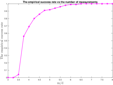
Figure 1: The empirical success rate for different $m/d$ based on $100$ random trails.

Example 2

In this example, we test the convergence rate of the Algorithm 1. We choose $d=1000$ and $m=7d$. The step size $\mu=0.01$. To show the robustness, we consider the noisy data model $y_{j}=\left\lvert\langle{{\bm{a}}_{j},{\bm{x}}}\rangle+b_{j}\right\rvert^{2}+\eta_{j}$ where the noise $\eta_{j}\sim{\mathcal{N}}(0,0.01^{2})$. The results are presented in Figure 2, which verifies the linear convergence of the Algorithm 1.

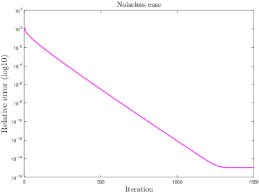
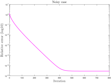
Figure 2: Relative error versus the number of iterations: (a) The noiseless measurements; (b) The noisy measurements.

5 Discussion

In this paper, we provide the characterization of a natural least squares formulation (1) for the affine phase retrieval problem. We show the loss function $f$ given in (1) is strongly convex on the entire space ${\mathbb{C}}^{d}$. This benign geometric structure allows the simple gradient descent algorithm to reconstruct the target signals with linear convergence rate.

There are some interesting problems for future research. First, Theorem 2.1 requires $m\gtrsim d\log d$ samples to guarantee the strongly convexity. Based on numerical experiments, we conjecture $m\gtrsim d$ samples are sufficient to ensure the property. It is interesting to see whether the gap can be closed. Second, our current analysis requires the measurements to be Gaussian random vectors. It is of practical interest to extend this result to other measurements, such as sub-Gaussian measurements, Fourier measurements and short-time Fourier measurements etc.

Appendix A Preliminaries and supporting lemmas

Lemma 3 (Chebyshev’s inequality)

For a random variable $X$ with finite variance $\sigma^{2}=\mbox{\rm Var}(X)$, we have

$${\mathbb{P}}\left(\left\lvert X-{\mathbb{E}}X\right\rvert\geq t\right)\leq\frac{\sigma^{2}}{t^{2}}\quad\mbox{for all}\quad t>0.$$

Lemma 4

(Vershynin2018, , Bernstein’s inequality) Let $X_{1},\ldots,X_{m}$ be independent, mean zero, sub-exponential random variables, and ${\bm{b}}=(b_{1},\ldots,b_{m})\in{\mathbb{R}}^{m}$. Then for any $t\geq 0$ it holds that

$${\mathbb{P}}\left\{\Big{|}\sum_{j=1}^{m}b_{j}X_{j}\Big{|}\geq t\right\}\leq 2\exp\left(-c\min\Big{(}\frac{t^{2}}{K^{2}\|{{\bm{b}}}\|_{2}^{2}},\frac{t}{K\|{\bm{b}}\|_{\infty}}\Big{)}\right),$$

where $c>0$ is an absolute constant and $K$ is the maximal sub-exponential norm, i.e., $K:=\mathrm{max}_{j}\|X_{j}\|_{\psi_{1}}$.

The following result is a complex version of Lemma 4.4.3 in Vershynin2018 and the proof is the same as that of Lemma 4.4.3 in Vershynin2018 .

Lemma 5

Let $M\in{\mathbb{C}}^{d\times d}$ be a Hermitian matrix and $\varepsilon\in[0,1/2)$. Then we have

$$\|{M}\|_{2}\leq\frac{1}{1-2\varepsilon}\cdot\sup_{{\bm{x}}\in\mathcal{N}}|\langle{M{\bm{x}},{\bm{x}}}\rangle|,$$

where $\mathcal{N}$ is a $\varepsilon$-net of the sphere $\mathbb{S}_{{\mathbb{C}}}^{d-1}$.

Lemma 6

(turstregion, , Lemma 21) Let ${\bm{a}}_{j}\in{\mathbb{C}}^{d},j=1,\ldots,m,$ be i.i.d complex Gaussian random vectors. Suppose that ${\bm{x}}\in{\mathbb{C}}^{d}$ is a fixed vector. For any $\epsilon\in(0,1)$ the following holds with probability at least $1-c_{a}\epsilon^{-2}m^{-1}-c_{b}\exp(-c_{c}\epsilon^{2}m/\log m)$:

$$\left\|\frac{1}{m}\sum_{j=1}^{m}\left\lvert{\bm{a}}_{j}^{*}{\bm{x}}\right\rvert^{2}{\bm{a}}_{j}{\bm{a}}_{j}^{*}-\big{(}{\bm{x}}{\bm{x}}^{*}+\|{{\bm{x}}}\|_{2}^{2}~{}I\big{)}\right\|\leq\epsilon\|{{\bm{x}}}\|^{2}$$

provided $m\geq C(\epsilon)d\log d$. Here $C(\epsilon)$ is a constant depending on $\epsilon$, $c_{a}$, $c_{b}$ and $c_{c}$ are positive absolute constants.

Lemma 7

(turstregion, , Lemma 22) Let ${\bm{a}}_{j}\in{\mathbb{C}}^{d},j=1,\ldots,m,$ be i.i.d complex Gaussian random vectors. For any $\epsilon\in(0,1)$ the followings hold with probability at least $1-c^{\prime}m^{-d}-c^{\prime\prime}\exp(-c(\epsilon)m)$:

$$\frac{1}{m}\sum_{j=1}^{m}\left\lvert{\bm{a}}_{j}^{*}{\bm{z}}\right\rvert^{2}\left\lvert{\bm{a}}_{j}^{*}\bm{v}\right\rvert^{2}\geq(1-\epsilon)\left(\|{\bm{v}}\|^{2}\|{{\bm{z}}}\|^{2}+\left\lvert\bm{v}^{*}{\bm{z}}\right\rvert^{2}\right)\quad\mbox{for all}\quad{\bm{z}},\bm{v}\in{\mathbb{C}}^{d},$$

$$\frac{1}{m}\sum_{j=1}^{m}\left(({\bm{a}}_{j}^{*}{\bm{z}})({\bm{v}}^{*}{\bm{a}}_{j})\right)_{\Re}^{2}\geq(1-\epsilon)\left(\frac{1}{2}\|{{\bm{z}}}\|_{2}^{2}\|{{\bm{v}}}\|_{2}^{2}+\frac{3}{2}\left(\Re({\bm{z}}^{*}{\bm{v}})\right)^{2}-\frac{1}{2}\left(\Im({\bm{z}}^{*}{\bm{v}})\right)^{2}\right)$$

$$\mbox{for all}\quad{\bm{z}},\;{\bm{v}}\in{\mathbb{C}}^{d},$$

provided $m\geq C(\epsilon)d\log d$. Here $C(\epsilon)$ and $c(\epsilon)$ are constants depending on $\epsilon$ and $c^{\prime}$, $c^{\prime\prime}$ are positive absolute constants.

The following lemma is an alternative version of Lemma 3.3 in huang2021a .

Lemma 8

Let $\eta\in{\mathbb{R}}^{m}$ be a fixed vector. Suppose that ${\bm{a}}_{j}\in{\mathbb{C}}^{d},j=1,\ldots,m$, are i.i.d. complex Gaussian random vectors. Then there exists a universal constant $C>0$ such that the following holds with probability at least $1-2\exp(-c_{0}d)$:

$$\|{\sum_{j=1}^{m}\eta_{j}({\bm{a}}_{j}{\bm{a}}_{j}^{*}-I)}\|_{2}\leq C\left(\sqrt{d}\|{\eta}\|_{2}+d\|{\eta}\|_{\infty}\right).$$

Here, $c_{0}>0$ is a universal constant.

Lemma 9

Assume that ${\bm{a}}_{j}\in{\mathbb{C}}^{d},j=1,\ldots,m,$ are i.i.d complex Gaussian random vectors. If $m\geq Cd$ for a universal constant $C>0$ then, with probability at least $1-3\exp(-cm)$, the following holds:

$$\frac{1}{m}\sum_{j=1}^{m}\left\lvert|{\bm{a}}_{j}^{*}{\bm{z}}+b_{j}|^{2}-|{\bm{a}}_{j}^{*}{\bm{w}}+b_{j}|^{2}\right\rvert\leq\frac{3}{2}\left(\|{{\bm{z}}}\|_{2}+\|{{\bm{w}}}\|_{2}+\frac{2\|{{\bm{b}}}\|_{2}}{\sqrt{m}}\right)\|{{\bm{z}}-{\bm{w}}}\|_{2}$$

for all ${\bm{z}},{\bm{w}}\in{\mathbb{C}}^{d}$ and ${\bm{b}}=(b_{1},\ldots,b_{m})^{\top}\in{\mathbb{C}}^{m}$. Here, $c$ is a positive absolute constants.

Proof

A simple calculation shows that

$$\frac{1}{m}\sum_{j=1}^{m}\left\lvert|{\bm{a}}_{j}^{*}{\bm{z}}+b_{j}|^{2}-|{\bm{a}}_{j}^{*}{\bm{w}}+b_{j}|^{2}\right\rvert$$ (34)

$$\leq\frac{1}{m}\sum_{j=1}^{m}\left\lvert|{\bm{a}}_{j}^{*}{\bm{z}}|^{2}-|{\bm{a}}_{j}^{*}{\bm{w}}|^{2}\right\rvert+\frac{2}{m}\sum_{j=1}^{m}|b_{j}|\left\lvert{\bm{a}}_{j}^{*}({\bm{z}}-{\bm{w}})\right\rvert$$

$$\leq\frac{1}{m}\sum_{j=1}^{m}\left\lvert|{\bm{a}}_{j}^{*}{\bm{z}}|^{2}-|{\bm{a}}_{j}^{*}{\bm{w}}|^{2}\right\rvert+\frac{2\|{{\bm{b}}}\|_{2}}{\sqrt{m}}\sqrt{\frac{1}{m}\sum_{j=1}^{m}|{\bm{a}}_{j}^{*}({\bm{z}}-{\bm{w}})|^{2}}.$$

We first consider the term $\frac{1}{m}\sum_{j=1}^{m}\left\lvert|{\bm{a}}_{j}^{*}{\bm{z}}|^{2}-|{\bm{a}}_{j}^{*}{\bm{w}}|^{2}\right\rvert$ in (34). According to Lemma 3.1 in phaselift , the following holds with probability at least $1-2\exp(-cm)$:

$$\frac{1}{m}\sum_{j=1}^{m}\left\lvert|{\bm{a}}_{j}^{*}{\bm{z}}|^{2}-|{\bm{a}}_{j}^{*}{\bm{w}}|^{2}\right\rvert \leq \frac{3}{2\sqrt{2}}\Big{\|}{\bm{z}}{\bm{z}}^{*}-{\bm{w}}{\bm{w}}^{*}\Big{\|}_{*}$$ (35)

$$\leq \frac{3}{2}\|{{\bm{z}}{\bm{z}}^{*}-{\bm{w}}{\bm{w}}^{*}}\|_{2}$$

$$\leq \frac{3}{2}(\|{{\bm{z}}}\|_{2}+\|{{\bm{w}}}\|_{2})\|{{\bm{z}}-{\bm{w}}}\|_{2}.$$

for all ${\bm{z}},{\bm{w}}\in{\mathbb{C}}^{d}$. Here, $\|\cdot\|_{*}$ denotes the nuclear norm.

We next turn to the second term in (34). We have

$$\frac{1}{m}\sum_{j=1}^{m}|{\bm{a}}_{j}^{*}({\bm{z}}-{\bm{w}})|^{2}\leq\Big{\|}\frac{1}{m}\sum_{j=1}^{m}{\bm{a}}_{j}{\bm{a}}_{j}^{*}\Big{\|}_{2}\Big{\|}{\bm{z}}-{\bm{w}}\Big{\|}_{2}^{2}\leq\frac{9}{4}\Big{\|}{\bm{z}}-{\bm{w}}\Big{\|}_{2}^{2},$$ (36)

where we use the fact that $\Big{\|}\frac{1}{m}\sum_{j=1}^{m}{\bm{a}}_{j}{\bm{a}}_{j}^{*}\Big{\|}_{2}\leq\frac{9}{4}$ with probability at least $1-\exp(-cm)$ in the last inequality.

Putting (36) and (35) into (34), we obtain that when $m\geq Cd$ then with probability at least $1-3\exp(-cm)$ it holds

$$\frac{1}{m}\sum_{j=1}^{m}\left\lvert|{\bm{a}}_{j}^{*}{\bm{z}}+b_{j}|^{2}-|{\bm{a}}_{j}^{*}{\bm{w}}+b_{j}|^{2}\right\rvert\leq\frac{3}{2}\left(\|{{\bm{z}}}\|_{2}+\|{{\bm{w}}}\|_{2}+\frac{2\|{{\bm{b}}}\|_{2}}{\sqrt{m}}\right)\|{{\bm{z}}-{\bm{w}}}\|_{2}$$

for all ${\bm{z}},{\bm{w}}\in{\mathbb{C}}^{d}$.

Lemma 10

Suppose that $\beta\geq 1$ is fixed constant. Assume ${\bm{a}}_{j}\in{\mathbb{C}}^{d},j=1,\ldots,m$, are i.i.d. complex Gaussian random vectors and ${\bm{b}}\in{\mathbb{C}}^{m}$ obeys $\sum_{j=1}^{m}|b_{j}|^{4}\lesssim m$ and $\|{{\bm{b}}}\|_{\infty}\leq\sqrt{\log m}$. For any $\epsilon\in(0,1)$, if $m\geq C\epsilon^{-2}\log(1/\epsilon)d\log m$ then with probability at least $1-2\exp(-c^{\prime}\epsilon^{2}m/\log m)-2\exp(-c^{\prime\prime}d)$ it holds that

$$\frac{1}{m}\sum_{j=1}^{m}|b_{j}|^{2}|{\bm{a}}_{j}^{*}{\bm{v}}|^{2}{\mathds{1}}_{|{\bm{a}}_{j}^{*}{\bm{v}}|\geq\beta}\leq\left(2\beta e^{-0.49\beta^{2}}+\epsilon\right)\cdot\frac{\|{{\bm{b}}}\|_{2}^{2}}{m}+\epsilon$$

for all ${\bm{v}}\in\mathbb{S}_{{\mathbb{C}}}^{d-1}$. Here, $C,c^{\prime},c^{\prime\prime}>0$ are universal constants and $~{}\mathbb{S}_{{\mathbb{C}}}^{d-1}:=\{{\bm{v}}\in{\mathbb{C}}^{d}:\|{\bm{v}}\|=1\}$.

Proof

Due to the non-Lipschitz of the indicator function ${\mathds{1}}_{|{\bm{a}}_{j}^{*}{\bm{v}}|\geq\beta}$, we introduce an auxiliary Lipschitz function to approximate it. Set

$$\chi(t):=\left\{\begin{array}[]{ll}t,&\mbox{if}\quad t\geq\beta^{2};\\ \frac{1}{\delta}t-(\frac{1}{\delta}-1)\beta^{2},&\mbox{if}\quad(1-\delta)\beta^{2}\leq t\leq\beta^{2};\\ 0,&\mbox{otherwise}.\end{array}\right.$$

Here $\delta\in(0,1)$ is a constant which will be chosen later. Then it is easy to check that

$$\frac{1}{m}\sum_{j=1}^{m}|b_{j}|^{2}|{\bm{a}}_{j}^{*}{\bm{v}}|^{2}{\mathds{1}}_{|{\bm{a}}_{j}^{*}{\bm{v}}|\geq\beta}\leq\frac{1}{m}\sum_{j=1}^{m}|b_{j}|^{2}\chi(|{\bm{a}}_{j}^{*}{\bm{v}}|^{2}).$$ (37)

For any fixed ${\bm{v}}_{0}\in\mathbb{S}_{{\mathbb{C}}}^{d-1}$, the terms $\chi(|{\bm{a}}_{j}^{*}{\bm{v}}_{0}|^{2})$ are independent sub-exponential random variables with the maximal sub-exponential norm being a constant. According to Bernstein’s inequality (Lemma 4), for any fixed $t\geq 0$ , it holds that

$${\mathbb{P}}\left\{\left\lvert\frac{1}{m}\sum_{j=1}^{m}|b_{j}|^{2}\chi(|{\bm{a}}_{j}^{*}{\bm{v}}_{0}|^{2})-\frac{\|{{\bm{b}}}\|_{2}^{2}}{m}\cdot{\mathbb{E}}\left(\chi(|{\bm{a}}_{1}^{*}{\bm{v}}_{0}|^{2})\right)\right\rvert\geq t\right\}\leq 2\exp\left(-c\min\Big{(}\frac{m^{2}t^{2}}{\sum_{j=1}^{m}|b_{j}|^{4}},\frac{mt}{\|{{\bm{b}}}\|_{\infty}^{2}}\Big{)}\right),$$ (38)

where $c>0$ is a universal constant. Recall that $\sum_{j=1}^{m}|b_{j}|^{4}\lesssim m\quad\mbox{and}\quad\|{{\bm{b}}}\|_{\infty}^{2}\lesssim\log m$. For any $0<\epsilon<1$, taking $t:=\epsilon/2$ in (38), we obtain that

$$\frac{1}{m}\sum_{j=1}^{m}|b_{j}|^{2}\chi(|{\bm{a}}_{j}^{*}{\bm{v}}_{0}|^{2})\leq\frac{\|{{\bm{b}}}\|_{2}^{2}}{m}\cdot{\mathbb{E}}\left(\chi(|{\bm{a}}_{1}^{*}{\bm{v}}_{0}|^{2})\right)+\frac{\epsilon}{2}$$ (39)

holds with probability at least $1-2\exp(-c_{1}\epsilon^{2}m/\log m)$, where $c_{1}>0$ is a universal constant.

We next show that (39) holds for any ${\bm{v}}\in{\mathbb{S}}_{{\mathbb{C}}}^{d-1}$. Suppose that $\mathcal{N}$ is a $\varepsilon_{0}$-net over ${\mathbb{S}}_{{\mathbb{C}}}^{d-1}$ with $\#\mathcal{N}\leq(1+\frac{2}{\varepsilon_{0}})^{2d}$. Then for any ${\bm{v}}\in{\mathbb{S}}_{{\mathbb{C}}}^{d-1}$, there exists a ${\bm{v}}_{0}\in\mathcal{N}$ such that $\|{{\bm{v}}-{\bm{v}}_{0}}\|_{2}\leq\varepsilon_{0}$. Note that $\chi(t)$ is a Lipschitz function with Lipschitz constant $1/\delta$. We obtain that if $m\geq C_{1}d\log m$ for a universal constant $C_{1}>0$ then

$$\left\lvert\frac{1}{m}\sum_{j=1}^{m}|b_{j}|^{2}\chi(|{\bm{a}}_{j}^{*}{\bm{v}}|^{2})-\frac{1}{m}\sum_{j=1}^{m}|b_{j}|^{2}\chi(|{\bm{a}}_{j}^{*}{\bm{v}}_{0}|^{2})\right\rvert$$ (40)

$$\leq\frac{1}{m\delta}\sum_{j=1}^{m}|b_{j}|^{2}\left\lvert|{\bm{a}}_{j}^{*}{\bm{v}}|^{2}-|{\bm{a}}_{j}^{*}{\bm{v}}_{0}|^{2}\right\rvert$$

$$\leq\frac{1}{m\delta}\sum_{j=1}^{m}|b_{j}|^{2}|{\bm{a}}_{j}^{*}{\bm{v}}|\left\lvert{\bm{a}}_{j}^{*}({\bm{v}}-{\bm{v}}_{0})\right\rvert+\frac{1}{m\delta}\sum_{j=1}^{m}|b_{j}|^{2}|{\bm{a}}_{j}^{*}{\bm{v}}_{0}|\left\lvert{\bm{a}}_{j}^{*}({\bm{v}}-{\bm{v}}_{0})\right\rvert$$

$$\leq\frac{1}{\delta}\left(\sqrt{\frac{1}{m}\sum_{j=1}^{m}|b_{j}|^{2}|{\bm{a}}_{j}^{*}{\bm{v}}|^{2}}+\sqrt{\frac{1}{m}\sum_{j=1}^{m}|b_{j}|^{2}|{\bm{a}}_{j}^{*}{\bm{v}}_{0}|^{2}}\right)\cdot\sqrt{\frac{1}{m}\sum_{j=1}^{m}|b_{j}|^{2}\left\lvert{\bm{a}}_{j}^{*}({\bm{v}}-{\bm{v}}_{0})\right\rvert^{2}}$$

$$\overset{(a)}{\lesssim}\frac{1}{\delta}\left(\frac{\|{{\bm{b}}}\|_{2}^{2}}{m}+\sqrt{\frac{1}{m}\sum_{j=1}^{m}|b_{j}|^{4}}+\frac{d\|{{\bm{b}}}\|_{\infty}^{2}}{m}\right)\varepsilon_{0}$$

$$\lesssim\frac{1}{\delta}\left(\frac{\|{{\bm{b}}}\|_{2}^{2}}{m}+1\right)\varepsilon_{0}.$$

Here, the inequality $(a)$ follows from Lemma 8 which says that, with probability at least $1-2\exp(-c_{2}d)$, it holds that

$$\sum_{j=1}^{m}|b_{j}|^{2}|{\bm{a}}_{j}^{*}{\bm{w}}|^{2}\leq{\bm{w}}^{*}\left(\sum_{j=1}^{m}|b_{j}|^{2}{\bm{a}}_{j}{\bm{a}}_{j}^{*}\right){\bm{w}}\lesssim\left(\|{{\bm{b}}}\|_{2}^{2}+\sqrt{d}\sqrt{\sum_{j=1}^{m}|b_{j}|^{4}}+d\|{{\bm{b}}}\|_{\infty}^{2}\right)\|{{\bm{w}}}\|_{2}^{2}$$

for all ${\bm{w}}\in{\mathbb{C}}^{d}$, where $c_{2}>0$ is a universal constant. Here, we use the fact that $\sum_{j=1}^{m}|b_{j}|^{4}\lesssim m$ and $\|{{\bm{b}}}\|_{\infty}^{2}\lesssim\log m$. Choosing $\varepsilon_{0}:=c_{3}\epsilon\delta$ in (40) for some universal constant $c_{3}>0$ and taking the union bound over $\mathcal{N}$, we obtain that

$$\frac{1}{m}\sum_{j=1}^{m}|b_{j}|^{2}\chi(|{\bm{a}}_{j}^{*}{\bm{v}}|^{2})\leq\frac{\|{{\bm{b}}}\|_{2}^{2}}{m}\cdot\left({\mathbb{E}}\left(\chi(|{\bm{a}}_{1}^{*}{\bm{v}}|^{2})\right)+\epsilon\right)+\epsilon$$ (41)

holds for all ${\bm{v}}\in\mathbb{S}_{{\mathbb{C}}}^{d-1}$ with probability at least

$$1-2(1+\frac{2}{\varepsilon_{0}})^{2d}\cdot\exp(-c_{1}\epsilon^{2}m/\log m)-2\exp(-c_{2}d)\geq 1-2\exp(-c^{\prime}\epsilon^{2}m/\log m)-2\exp(-c_{2}d)$$

provided $m\geq C^{\prime}\epsilon^{-2}\log(\epsilon^{-1}\delta^{-1})~{}d\log m$, where $C^{\prime},c^{\prime}>0$ are universal constants.

We next turn to ${\mathbb{E}}\left(\chi(|{\bm{a}}_{1}^{*}{\bm{v}}|^{2})\right)$ in (41). A simple calculation shows that

$${\mathbb{E}}\left(|{\bm{a}}_{1}^{*}{\bm{v}}|^{2}{\mathds{1}}_{|{\bm{a}}_{j}^{*}{\bm{v}}|\geq\gamma}\right)\leq\sqrt{\frac{2}{\pi}}\left(\gamma+\frac{1}{\gamma}\right)e^{-\gamma^{2}/2}$$ (42)

for any $\gamma>0$. Note that ${\mathbb{E}}\left(\chi(|{\bm{a}}_{1}^{*}{\bm{v}}|^{2})\right)\leq{\mathbb{E}}\left(|{\bm{a}}_{1}^{*}{\bm{v}}|^{2}{\mathds{1}}_{|{\bm{a}}_{j}^{*}{\bm{v}}|\geq(1-\delta)\beta}\right)$. Set $\delta:=0.01$ and $\gamma:=(1-\delta)\beta$. It then follows from (37), (41) and (42) that with probability at least $1-2\exp(-c^{\prime}\epsilon^{2}m/\log m)-2\exp(-c_{2}d)$, it holds

$$\frac{1}{m}\sum_{j=1}^{m}|b_{j}|^{2}|{\bm{a}}_{j}^{*}{\bm{v}}|^{2}{\mathds{1}}_{|{\bm{a}}_{j}^{*}{\bm{v}}|\geq\beta}\leq\left(2\beta e^{-0.49\beta^{2}}+\epsilon\right)\cdot\frac{\|{{\bm{b}}}\|_{2}^{2}}{m}+\epsilon$$

for all ${\bm{v}}\in\mathbb{S}_{{\mathbb{C}}}^{d-1}$, provided $m\geq C\epsilon^{-2}\log(1/\epsilon)~{}d\log m$. Here, $C>0$ is a universal constant. We complete the proof.

Lemma 11

Suppose that ${\bm{a}}_{j}\in{\mathbb{C}}^{d},j=1,\ldots,m$, are i.i.d. complex Gaussian random vectors. Assume that ${\bm{b}}\in{\mathbb{C}}^{m}$ is a vector obeying $\sum_{j=1}^{m}|b_{j}|^{4}\lesssim m$ and $\|{{\bm{b}}}\|_{\infty}\lesssim\sqrt{\log m}$. For any $\epsilon\in(0,1)$, if $m\geq c(\epsilon)d\log m$ then the following holds with probability at least $1-6\exp(-c^{\prime}(\epsilon)m/\log m)-6\exp(-c^{\prime\prime}d)$:

$$\left\lvert\frac{1}{m}\sum_{j=1}^{m}\left(\bar{b}_{j}({\bm{a}}_{j}^{*}{\bm{z}})\right)_{\Re}|{\bm{a}}_{j}^{*}{\bm{v}}|^{2}\right\rvert\leq\epsilon\left(\frac{\|{{\bm{b}}}\|_{2}}{\sqrt{m}}+1\right)\left(1+\left(\frac{1}{m}\sum_{j=1}^{m}|{\bm{a}}_{j}^{*}{\bm{z}}|^{2}|{\bm{a}}_{j}^{*}{\bm{v}}|^{2}\right)^{\frac{1}{2}}\right)$$

for all ${\bm{z}},{\bm{v}}\in\mathbb{S}_{{\mathbb{C}}}^{d-1}$, where $~{}\mathbb{S}_{{\mathbb{C}}}^{d-1}:=\{{\bm{x}}\in{\mathbb{C}}^{d}:\|{\bm{x}}\|=1\}$, $c^{\prime\prime}$ is a positive universal constant and $c(\epsilon)$, $c^{\prime}(\epsilon)$ are positive constants depending only on $\epsilon$.

Proof

Suppose that $\phi\in C_{c}^{\infty}(\mathbb{R})$ is a Lipschitz continuous function satisfying $0\leq\phi(x)\leq 1$ for all $x\in\mathbb{R}$. We furthermore require $\phi(x)=1$ for $|x|\leq 1$ and $\phi(x)=0$ for $|x|\geq 2$. For any $\beta>0$, we have

$$\left\lvert\frac{1}{m}\sum_{j=1}^{m}\left(\bar{b}_{j}({\bm{a}}_{j}^{*}{\bm{z}})\right)_{\Re}|{\bm{a}}_{j}^{*}{\bm{v}}|^{2}\right\rvert$$ (43)

$$\leq\left\lvert\frac{1}{m}\sum_{j=1}^{m}\left(\bar{b}_{j}({\bm{a}}_{j}^{*}{\bm{z}})\right)_{\Re}|{\bm{a}}_{j}^{*}{\bm{v}}|^{2}\phi\left(\frac{|{\bm{a}}_{j}^{*}{\bm{v}}|}{\beta}\right)\right\rvert+\left\lvert\frac{1}{m}\sum_{j=1}^{m}\left(\bar{b}_{j}({\bm{a}}_{j}^{*}{\bm{z}})\right)_{\Re}|{\bm{a}}_{j}^{*}{\bm{v}}|^{2}\left(1-\phi\left(\frac{|{\bm{a}}_{j}^{*}{\bm{v}}|}{\beta}\right)\right)\right\rvert$$

$$\leq\left\lvert\frac{1}{m}\sum_{j=1}^{m}b_{j,\Re}({\bm{a}}_{j}^{*}{\bm{z}})_{\Re}|{\bm{a}}_{j}^{*}{\bm{v}}|^{2}\phi\left(\frac{|{\bm{a}}_{j}^{*}{\bm{v}}|}{\beta}\right)\right\rvert+\left\lvert\frac{1}{m}\sum_{j=1}^{m}b_{j,\Im}({\bm{a}}_{j}^{*}{\bm{z}})_{\Im}|{\bm{a}}_{j}^{*}{\bm{v}}|^{2}\phi\left(\frac{|{\bm{a}}_{j}^{*}{\bm{v}}|}{\beta}\right)\right\rvert$$

$$\quad+\frac{1}{m}\sum_{j=1}^{m}|b_{j}||{\bm{a}}_{j}^{*}{\bm{z}}||{\bm{a}}_{j}^{*}{\bm{v}}|^{2}{\mathds{1}}_{\left\{|{\bm{a}}_{j}^{*}{\bm{v}}|\geq\beta\right\}}:=T_{1}+T_{2}+r.$$

We claim that for any $\epsilon\in(0,1)$ there exists a sufficiently large $\beta>1$ such that if $m\geq c(\epsilon)d\log m$ then, with probability at least $1-6\exp(-c^{\prime}(\epsilon)m/\log m)-6\exp(c^{\prime\prime}d)$, the followings hold

$$T_{1}\leq\frac{\epsilon}{2}\cdot\left(\frac{\|{{\bm{b}}}\|_{2}}{\sqrt{m}}+1\right),\quad T_{2}\leq\frac{\epsilon}{2}\cdot\left(\frac{\|{{\bm{b}}}\|_{2}}{\sqrt{m}}+1\right),$$ (44)

$$r\leq\epsilon\left(\frac{\|{{\bm{b}}}\|_{2}}{\sqrt{m}}+1\right)\left(\frac{1}{m}\sum_{j=1}^{m}|{\bm{a}}_{j}^{*}{\bm{z}}|^{2}|{\bm{a}}_{j}^{*}{\bm{v}}|^{2}\right)^{\frac{1}{2}}$$ (45)

for all ${\bm{z}},{\bm{v}}\in\mathbb{S}_{{\mathbb{C}}}^{d-1}$. Here $c(\epsilon),c^{\prime}(\epsilon)$ are constants depending on $\epsilon$ and $c^{\prime\prime}$ is a positive universal constant. Combining (43), (44) and (45), we arrive at the conclusion, i.e,

$$\left\lvert\frac{1}{m}\sum_{j=1}^{m}\left(\bar{b}_{j}({\bm{a}}_{j}^{*}{\bm{z}})\right)_{\Re}|{\bm{a}}_{j}^{*}{\bm{v}}|^{2}\right\rvert\leq\epsilon\left(\frac{\|{{\bm{b}}}\|_{2}}{\sqrt{m}}+1\right)\left(1+\left(\frac{1}{m}\sum_{j=1}^{m}|{\bm{a}}_{j}^{*}{\bm{z}}|^{2}|{\bm{a}}_{j}^{*}{\bm{v}}|^{2}\right)^{\frac{1}{2}}\right)$$

holds for all ${\bm{z}},{\bm{v}}\in\mathbb{S}_{{\mathbb{C}}}^{d-1}$.

It remains to prove the claims (44) and (45). We first present an upper bound for $T_{1}$. For any fixed ${\bm{z}}_{0},{\bm{v}}_{0}\in\mathbb{S}_{{\mathbb{C}}}^{d-1}$, due to the cut-off $\phi\left(\frac{|{\bm{a}}_{j}^{*}{\bm{v}}|}{\beta}\right)$, the terms $({\bm{a}}_{j}^{*}{\bm{z}}_{0})_{\Re}|{\bm{a}}_{j}^{*}{\bm{v}}_{0}|^{2}\phi\left(\frac{|{\bm{a}}_{j}^{*}{\bm{v}}_{0}|}{\beta}\right)$ are centered, independent sub-gaussian random variables with the sub-gaussian norm $O(\beta)$. According to Hoeffding’s inequality, we obtain that the following holds with probability at least $1-2\exp(-c\epsilon^{2}\beta^{-2}m)$

$$\left\lvert\frac{1}{m}\sum_{j=1}^{m}b_{j,\Re}({\bm{a}}_{j}^{*}{\bm{z}}_{0})_{\Re}|{\bm{a}}_{j}^{*}{\bm{v}}_{0}|^{2}\phi\left(\frac{|{\bm{a}}_{j}^{*}{\bm{v}}_{0}|}{\beta}\right)\right\rvert\leq\frac{\epsilon\|{{\bm{b}}}\|_{2}}{4\sqrt{m}},$$ (46)

where $c>0$ is a universal constant. We next show that (46) holds for all unit vectors ${\bm{z}},{\bm{v}}\in{\mathbb{S}}_{{\mathbb{C}}}^{d-1}$. We adopt a basic version of a $\delta$-net argument to show that. We assume that $\mathcal{N}$ is a $\delta$-net of the unit complex sphere in ${\mathbb{S}}_{{\mathbb{C}}}^{d-1}$ and hence the covering number $\#\mathcal{N}\leq(1+\frac{2}{\delta})^{2d}$. For any ${\bm{z}},{\bm{v}}\in\mathbb{S}_{{\mathbb{C}}}^{d-1}$, there exists a ${\bm{z}}_{0},{\bm{v}}_{0}\in\mathcal{N}\times\mathcal{N}$ such that $\|{{\bm{z}}-{\bm{z}}_{0}}\|_{2}\leq\delta$ and $\|{{\bm{v}}-{\bm{v}}_{0}}\|_{2}\leq\delta$. Noting $f(\tau):=\tau^{2}\phi(\tau/\beta)$ is a bounded function with Lipschitz constant $O(\beta)$, we obtain that

$$\Big{|}\frac{1}{m}\sum_{j=1}^{m}b_{j,\Re}({\bm{a}}_{j}^{*}{\bm{z}})_{\Re}|{\bm{a}}_{j}^{*}{\bm{v}}|^{2}\phi\left(\frac{|{\bm{a}}_{j}^{*}{\bm{v}}|}{\beta}\right)-\frac{1}{m}\sum_{j=1}^{m}b_{j,\Re}({\bm{a}}_{j}^{*}{\bm{z}}_{0})_{\Re}|{\bm{a}}_{j}^{*}{\bm{v}}_{0}|^{2}\phi\left(\frac{|{\bm{a}}_{j}^{*}{\bm{v}}_{0}|}{\beta}\right)\Big{|}$$

$$\leq\frac{1}{m}\sum_{j=1}^{m}|b_{j,\Re}||{\bm{a}}_{j}^{*}{\bm{v}}|^{2}\phi\left(\frac{|{\bm{a}}_{j}^{*}{\bm{v}}|}{\beta}\right)\left\lvert{\bm{a}}_{j}^{*}{\bm{z}}-{\bm{a}}_{j}^{*}{\bm{z}}_{0}\right\rvert$$

$$\quad+\frac{1}{m}\sum_{j=1}^{m}|b_{j,\Re}||{\bm{a}}_{j}^{*}{\bm{z}}_{0}|~{}\Big{|}|{\bm{a}}_{j}^{*}{\bm{v}}|^{2}\phi\left(\frac{|{\bm{a}}_{j}^{*}{\bm{v}}|}{\beta}\right)-|{\bm{a}}_{j}^{*}{\bm{v}}_{0}|^{2}\phi\left(\frac{|{\bm{a}}_{j}^{*}{\bm{v}}_{0}|}{\beta}\right)\Big{|}$$

$$\lesssim\frac{\beta^{2}}{m}\sum_{j=1}^{m}|b_{j,\Re}|\left\lvert{\bm{a}}_{j}^{*}{\bm{z}}-{\bm{a}}_{j}^{*}{\bm{z}}_{0}\right\rvert+\frac{\beta}{m}\sum_{j=1}^{m}|b_{j,\Re}||{\bm{a}}_{j}^{*}{\bm{z}}_{0}|\left\lvert{\bm{a}}_{j}^{*}{\bm{v}}-{\bm{a}}_{j}^{*}{\bm{v}}_{0}\right\rvert$$

$$\leq\frac{\beta^{2}}{m}\|{{\bm{b}}}\|_{2}\sqrt{\sum_{j=1}^{m}\lvert{\bm{a}}_{j}^{*}({\bm{z}}-{\bm{z}}_{0})\rvert^{2}}+\frac{\beta}{m}\sqrt{\sum_{j=1}^{m}|b_{j}|\lvert{\bm{a}}_{j}^{*}{\bm{z}}_{0}\rvert^{2}}\cdot\sqrt{\sum_{j=1}^{m}|b_{j}|\lvert{\bm{a}}_{j}^{*}({\bm{v}}-{\bm{v}}_{0})\rvert^{2}}$$

$$\lesssim\frac{\beta^{2}\|{{\bm{b}}}\|_{2}}{\sqrt{m}}\|{{\bm{z}}-{\bm{z}}_{0}}\|_{2}+\beta\left(\frac{\|{{\bm{b}}}\|_{2}}{\sqrt{m}}+1\right)\|{{\bm{v}}-{\bm{v}}_{0}}\|_{2}\leq 2\left(\frac{\|{{\bm{b}}}\|_{2}}{\sqrt{m}}+1\right)\beta^{2}\delta,$$

where the fourth inequality follows from Lemma 8 which says, with probability at least $1-2\exp(-c_{1}d)$ for a universal constant $c_{1}>0$, the following holds

$$\sum_{j=1}^{m}|b_{j}||{\bm{a}}_{j}^{*}{\bm{w}}|^{2}={\bm{w}}^{*}\left(\sum_{j=1}^{m}|b_{j}|{\bm{a}}_{j}{\bm{a}}_{j}^{*}\right){\bm{w}} \lesssim \left(\sum_{j=1}^{m}|b_{j}|+\sqrt{d}\|{{\bm{b}}}\|_{2}+d\|{{\bm{b}}}\|_{\infty}\right)\|{{\bm{w}}}\|_{2}^{2}$$

$$\lesssim \left(\sqrt{m}\|{{\bm{b}}}\|_{2}+m\right)\|{{\bm{w}}}\|_{2}^{2}\quad\mbox{for all}\quad{\bm{w}}\in{\mathbb{C}}^{d},$$

provided $\sum_{j=1}^{m}|b_{j}|\lesssim m$, $\|{{\bm{b}}}\|_{\infty}\lesssim\sqrt{\log m}$ and $m\gtrsim d\log m$. Here, we use the fact that

$$\sum_{j=1}^{m}|b_{j}|\leq\sqrt{m}\sqrt{\sum_{j=1}^{m}|b_{j}|^{2}}\leq\sqrt{m}\sqrt[4]{m\sum_{j=1}^{m}|b_{j}|^{4}}\lesssim m.$$

Choosing $\delta=c_{2}\epsilon/\beta^{2}$ for some universal constant $c_{2}>0$ and taking the union bound, we obtain that

$$T_{1}=\left\lvert\frac{1}{m}\sum_{j=1}^{m}b_{j,\Re}({\bm{a}}_{j}^{*}{\bm{z}})_{\Re}|{\bm{a}}_{j}^{*}{\bm{v}}|^{2}\phi\left(\frac{|{\bm{a}}_{j}^{*}{\bm{v}}|}{\beta}\right)\right\rvert\leq\left(\frac{\|{{\bm{b}}}\|_{2}}{\sqrt{m}}+1\right)\cdot\frac{\epsilon}{2}\quad\mbox{for all}\quad{\bm{z}},{\bm{v}}\in\mathbb{S}_{{\mathbb{C}}}^{d-1}$$

holds with probability at least

$$1-2(1+\frac{2}{\delta})^{2d}\cdot\exp(-c\epsilon^{2}\beta^{-2}m)-2\exp(-c_{1}d)\geq 1-2\exp(-c_{3}\epsilon^{2}\beta^{-2}m)-2\exp(-c_{1}d)$$

provided $m\geq C\cdot(\beta/\epsilon)^{2}\log(\beta/\epsilon)d\log m$. Here, $C$ and $c_{3}$ are positive universal constants. Using the similar argument as above, we obtain that the following holds with probability at least $1-2\exp(-c_{3}\epsilon^{2}\beta^{-2}m)-2\exp(-c_{1}d)$:

$$T_{2}=\left\lvert\frac{1}{m}\sum_{j=1}^{m}b_{j,\Im}({\bm{a}}_{j}^{*}{\bm{z}})_{\Im}|{\bm{a}}_{j}^{*}{\bm{v}}|^{2}\phi\left(\frac{|{\bm{a}}_{j}^{*}{\bm{v}}|}{\beta}\right)\right\rvert\leq\left(\frac{\|{{\bm{b}}}\|_{2}}{\sqrt{m}}+1\right)\cdot\frac{\epsilon}{2}\quad\mbox{for all}\quad{\bm{z}},{\bm{v}}\in\mathbb{S}_{{\mathbb{C}}}^{d-1}$$

provided $m\geq C\cdot(\beta/\epsilon)^{2}\log(\beta/\epsilon)d\log m$.

Finally, we turn to prove the claim (45). We use Cauchy-Schwarz inequality to obtain that

$$\frac{1}{m}\sum_{j=1}^{m}|b_{j}||{\bm{a}}_{j}^{*}{\bm{z}}||{\bm{a}}_{j}^{*}{\bm{v}}|^{2}{\mathds{1}}_{\left\{|{\bm{a}}_{j}^{*}{\bm{v}}|\geq\beta\right\}}\leq\sqrt{\frac{1}{m}\sum_{j=1}^{m}|{\bm{a}}_{j}^{*}{\bm{z}}|^{2}|{\bm{a}}_{j}^{*}{\bm{v}}|^{2}}\sqrt{\frac{1}{m}\sum_{j=1}^{m}|b_{j}|^{2}|{\bm{a}}_{j}^{*}{\bm{v}}|^{2}{\mathds{1}}_{|{\bm{a}}_{j}^{*}{\bm{v}}|\geq\beta}}.$$ (47)

Recall that $\sum_{j=1}^{m}|b_{j}|^{4}\lesssim m$ and $\|{\bm{b}}\|_{\infty}\lesssim\sqrt{m}$. According to Lemma 10, we obtain that if $m\geq C_{1}\epsilon^{-4}\log(1/\epsilon^{2})d\log m$ then, with probability at least $1-2\exp(-c_{4}\epsilon^{4}m/\log m)-2\exp(-c_{5}d)$ , the following holds

$$\frac{1}{m}\sum_{j=1}^{m}|b_{j}|^{2}|{\bm{a}}_{j}^{*}{\bm{v}}|^{2}{\mathds{1}}_{|{\bm{a}}_{j}^{*}{\bm{v}}|\geq\beta} \leq\left(2\beta e^{-0.49\beta^{2}}+\frac{\epsilon^{2}}{2}\right)\cdot\frac{\|{{\bm{b}}}\|_{2}^{2}}{m}+\frac{\epsilon^{2}}{2}$$ (48)

$$\leq\left(\frac{\|{{\bm{b}}}\|_{2}^{2}}{m}+1\right)\cdot\epsilon^{2}\leq\left(\frac{\|{{\bm{b}}}\|_{2}}{\sqrt{m}}+1\right)\epsilon$$

for all ${\bm{v}}\in\mathbb{S}_{{\mathbb{C}}}^{d-1}$, where $C_{1},c_{4}$ and $c_{5}$ are positive universal constants. Here, in the second inequality we take $\beta$ to be sufficiently large (depending only on $\epsilon$). Combining (47) and (48), we arrive at (45).

Lemma 12

Suppose that ${\bm{a}}_{j}\in{\mathbb{C}}^{d},j=1,\ldots,m$, are i.i.d. complex Gaussian random vectors. Assume that ${\bm{b}}\in{\mathbb{C}}^{m}$ satisfies $\sum_{j=1}^{m}|b_{j}|^{4}\lesssim m$ and $\|{{\bm{b}}}\|_{\infty}\lesssim\sqrt{\log m}$. Assume that ${\bm{x}}\in{\mathbb{C}}^{d}$ is a fixed vector. For any $\epsilon\in(0,1)$, if $m\geq C_{1}\epsilon^{-2}d\log m$ then, with probability at least $1-2\exp(-c^{\prime}\epsilon^{2}m/\log m)-c^{\prime\prime}\epsilon^{-2}m^{-1}$, it holds that

$$\left\|\frac{1}{m}\sum_{j=1}^{m}\left(\bar{b}_{j}({\bm{a}}_{j}^{*}{\bm{x}})\right)_{\Re}{\bm{a}}_{j}{\bm{a}}_{j}^{*}\right\|_{2}\leq\epsilon\left(\frac{\|{{\bm{b}}}\|_{2}}{\sqrt{m}}+1\right)\|{{\bm{x}}}\|_{2}.$$

Here, $C_{1},c^{\prime}$ and $c^{\prime\prime}$ are positive universal constants.

Proof

We assume that $\mathcal{N}$ is a $1/4$-net of the complex unit sphere ${\mathbb{S}}_{{\mathbb{C}}}^{d-1}$ with the cardinality $\#\mathcal{N}\leq 9^{2d}$. According to Lemma 5, we have

$$\left\|\frac{1}{m}\sum_{j=1}^{m}\left(\bar{b}_{j}({\bm{a}}_{j}^{*}{\bm{x}})\right)_{\Re}{\bm{a}}_{j}{\bm{a}}_{j}^{*}\right\|_{2}\leq 2\max_{{\bm{v}}\in\mathcal{N}}\Big{|}\frac{1}{m}\sum_{j=1}^{m}\left(\bar{b}_{j}({\bm{a}}_{j}^{*}{\bm{x}})\right)_{\Re}|{\bm{a}}_{j}^{*}{\bm{v}}|^{2}\Big{|}.$$

Without loss of generality, we assume ${\bm{x}}={\bm{e}}_{1}$. Then

$$\frac{1}{m}\sum_{j=1}^{m}\left(\bar{b}_{j}({\bm{a}}_{j}^{*}{\bm{x}})\right)_{\Re}|{\bm{a}}_{j}^{*}{\bm{v}}|^{2} =\frac{1}{m}\left\lvert v_{1}\right\rvert^{2}\sum_{j=1}^{m}\left(\bar{b}_{j}\bar{a}_{j,1}\right)_{\Re}|\bar{a}_{j,1}|^{2}+\frac{1}{m}\sum_{j=1}^{m}\left(\bar{b}_{j}\bar{a}_{j,1}\right)_{\Re}|\tilde{{\bm{a}}}_{j}^{*}\tilde{{\bm{v}}}|^{2}$$ (49)

where $\tilde{{\bm{a}}}_{j},\tilde{{\bm{v}}}\in{\mathbb{C}}^{d-1}$ are generated by deleting the first entry of the vector ${\bm{a}}_{j}$ and ${\bm{v}}$, respectively. For the first term, since ${\bm{a}}_{j}$ are standard complex Gaussian random variables, a simple calculation shows that

$$\mbox{Var}\left(\left(\bar{b}_{j}\bar{a}_{j,1}\right)_{\Re}|\bar{a}_{j,1}|^{2}\right)\leq 3\left\lvert{\bm{b}}_{j}\right\rvert^{2}.$$

It then follows from Chebyshev’s inequality (Lemma 3) that

$${\mathbb{P}}\left(\left\lvert\frac{1}{m}\sum_{j=1}^{m}\left(\bar{b}_{j}\bar{a}_{j,1}\right)_{\Re}|\bar{a}_{j,1}|^{2}\right\rvert\geq t\right)\leq\frac{3\|{{\bm{b}}}\|_{2}^{2}}{m^{2}t^{2}}.$$ (50)

For any $0<\epsilon<1$, taking $t:=\epsilon\|{{\bm{b}}}\|_{2}/\sqrt{m}$ in (50), we obtain that the following holds

$$\left\lvert\frac{1}{m}\sum_{j=1}^{m}\left(\bar{b}_{j}\bar{a}_{j,1}\right)_{\Re}|\bar{a}_{j,1}|^{2}\right\rvert\leq\frac{\epsilon\|{{\bm{b}}}\|_{2}}{\sqrt{m}}$$ (51)

with probability at least $1-3\epsilon^{-2}m^{-1}$. We next turn to the term $\frac{1}{m}\sum_{j=1}^{m}\left(\bar{b}_{j}\bar{a}_{j,1}\right)_{\Re}|\tilde{{\bm{a}}}_{j}^{*}\tilde{{\bm{v}}}|^{2}$ in (49). We note that

$$\frac{1}{m}\sum_{j=1}^{m}\left(\bar{b}_{j}\bar{a}_{j,1}\right)_{\Re}|\tilde{{\bm{a}}}_{j}^{*}\tilde{{\bm{v}}}|^{2}=\frac{1}{m}\sum_{j=1}^{m}b_{j,\Re}a_{j,1,\Re}|\tilde{{\bm{a}}}_{j}^{*}\tilde{{\bm{v}}}|^{2}-\frac{1}{m}\sum_{j=1}^{m}b_{j,\Im}a_{j,1,\Im}|\tilde{{\bm{a}}}_{j}^{*}\tilde{{\bm{v}}}|^{2}.$$

For any fixed $\tilde{{\bm{v}}}_{0}\in{\mathbb{C}}^{d-1}$, the terms $|\tilde{{\bm{a}}}_{j}^{*}\tilde{{\bm{v}}}_{0}|^{2}-\|{\tilde{{\bm{v}}}_{0}}\|_{2}^{2}$ are centered subexponential random variables with the maximal subexponential norm $K:=C\|{\tilde{{\bm{v}}}_{0}}\|_{2}^{2}$ where $C>0$ is a universal constant. Furthermore, $|\tilde{{\bm{a}}}_{j}^{*}\tilde{{\bm{v}}}_{0}|^{2}$ are independent with $a_{j,1}$. We use Bernstein’s inequality to obtain that

$${\mathbb{P}}\left(\frac{1}{m}\sum_{j=1}^{m}b_{j,\Re}a_{j,1,\Re}\Big{(}|\tilde{{\bm{a}}}_{j}^{*}\tilde{{\bm{v}}}_{0}|^{2}-\|{\tilde{{\bm{v}}}_{0}}\|_{2}^{2}\Big{)}\geq t\|{\tilde{{\bm{v}}}_{0}}\|_{2}^{2}\right)$$

$$\quad\leq 2\exp\left(-c\min\left(\frac{m^{2}t^{2}}{\sum_{j=1}^{m}b_{j,\Re}^{2}a_{j,1,\Re}^{2}},\frac{mt}{\max_{j\in[m]}\left\lvert b_{j,\Re}\right\rvert\cdot\left\lvert a_{j,1,\Re}\right\rvert}\right)\right),$$

where $c>0$ is a universal constant. Taking $t:=\epsilon/2$, together with the union bound over $\mathcal{N}$, we obtain that

$${\mathbb{P}}\left(\frac{1}{m}\sum_{j=1}^{m}b_{j,\Re}a_{j,1,\Re}\Big{(}|\tilde{{\bm{a}}}_{j}^{*}\tilde{{\bm{v}}}|^{2}-\|{\tilde{{\bm{v}}}}\|_{2}^{2}\Big{)}\geq\frac{\epsilon}{2}\|{\tilde{{\bm{v}}}}\|_{2}^{2}\right)$$ (52)

$$\leq 2\exp\left(-4c\min\left(\frac{m^{2}\epsilon^{2}}{\sum_{j=1}^{m}b_{j,\Re}^{2}a_{j,1,\Re}^{2}},\frac{m\epsilon}{\max_{j\in[m]}\left\lvert b_{j,\Re}\right\rvert\cdot\left\lvert a_{j,1,\Re}\right\rvert}\right)+5d\right)$$

for all ${\bm{v}}\in\mathcal{N}$. By Chebyshev’s inequality, we obtain that the following holds with probability at least $1-\epsilon^{-2}m^{-1}$

$$\left\lvert\frac{1}{m}\sum_{j=1}^{m}b_{j,\Re}a_{j,1,\Re}\right\rvert\|{\tilde{{\bm{v}}}}\|_{2}^{2}\leq\frac{\epsilon\|{{\bm{b}}_{\Re}}\|_{2}}{\sqrt{m}}\|{\tilde{{\bm{v}}}}\|_{2}^{2}.$$ (53)

Similarly, the Chebyshev’s inequality implies

$${\mathbb{P}}\left(\left\lvert\sum_{j=1}^{m}b_{j,\Re}^{2}a_{j,1,\Re}^{2}-\frac{1}{2}\|{{\bm{b}}_{\Re}}\|_{2}^{2}\right\rvert\geq m\right)\leq\frac{\sum_{j=1}^{m}|b_{j}|^{4}}{m^{2}}\lesssim\frac{1}{m}$$ (54)

provided $\sum_{j=1}^{m}|b_{j}|^{4}\lesssim m$. Moreover, a union bound gives

$$\max_{1\leq j\leq m}|a_{j,1}|\leq\sqrt{10\log m}$$ (55)

with probability at least $1-m^{-2}$. Putting (53), (54) and (55) into (52), we obtain that, with probability at least $1-2\exp(-c_{1}\epsilon^{2}m/\log m)-c_{2}\epsilon^{-2}m^{-1}-m^{-2}$, it holds

$$\left\lvert\frac{1}{m}\sum_{j=1}^{m}b_{j,\Re}a_{j,1,\Re}|\tilde{{\bm{a}}}_{j}^{*}\tilde{{\bm{v}}}|^{2}\right\rvert\leq\left(\frac{\|{{\bm{b}}_{\Re}}\|_{2}}{\sqrt{m}}+\frac{1}{2}\right)\epsilon\|{\tilde{{\bm{v}}}}\|_{2}^{2}\quad\mbox{for all}\quad{\bm{v}}\in\mathcal{N}$$ (56)

provided $\|{{\bm{b}}}\|_{2}\leq\sqrt[4]{m\sum_{j=1}^{m}|b_{j}|^{4}}\lesssim\sqrt{m}$, $\|{{\bm{b}}}\|_{\infty}\lesssim\sqrt{\log m}$ and $m\geq C_{1}\epsilon^{-2}d\log m$. Here, $C_{1},c_{1}$ and $c_{2}$ are positive universal constants. Using the same argument as above, we obtain that

$$\left\lvert\frac{1}{m}\sum_{j=1}^{m}b_{j,\Im}a_{j,1,\Im}|\tilde{{\bm{a}}}_{j}^{*}\tilde{{\bm{v}}}|^{2}\right\rvert\leq\left(\frac{\|{{\bm{b}}_{\Im}}\|_{2}}{\sqrt{m}}+\frac{1}{2}\right)\epsilon\|{\tilde{{\bm{v}}}}\|_{2}^{2}\quad\mbox{for all}\quad{\bm{v}}\in\mathcal{N}.$$ (57)

Combining (51), (56) and (57), we obtain that

$$\frac{1}{m}\sum_{j=1}^{m}\left(\bar{b}_{j}({\bm{a}}_{j}^{*}{\bm{x}})\right)_{\Re}|{\bm{a}}_{j}^{*}{\bm{v}}|^{2}\leq\left(\frac{\|{{\bm{b}}}\|_{2}}{\sqrt{m}}+1\right)\epsilon\|{{\bm{v}}}\|_{2}^{2}\quad\mbox{for all}\quad{\bm{v}}\in{\mathcal{N}}$$

holds with probability at least $1-2\exp(-c^{\prime}\epsilon^{2}m/\log m)-c^{\prime\prime}\epsilon^{-2}m^{-1}$, provided $m\geq C_{1}\epsilon^{-2}d\log m$. Here, $c^{\prime}>0$ and $c^{\prime\prime}>0$ are universal constants. This completes the proof.

Lemma 13

Suppose that ${\bm{a}}_{j}\in{\mathbb{C}}^{d},j=1,\ldots,m$, are i.i.d. complex Gaussian random vectors. Assume that ${\bm{b}}\in{\mathbb{C}}^{m}$ which satisfies $\sum_{j=1}^{m}|b_{j}|^{4}\lesssim m$ and $\|{{\bm{b}}}\|_{\infty}\leq\sqrt{\log m}$. For any $\epsilon\in(0,1)$, if $m\geq C^{\prime\prime}\epsilon^{-2}\log(1/\epsilon)~{}d\log m$ then, with probability at least $1-6\exp(-c^{\prime}\epsilon^{2}m/\log m)-6\exp(-c^{\prime\prime}d)$, it holds that

$$\frac{1}{m}\sum_{j=1}^{m}\left(\bar{b}_{j}({\bm{a}}_{j}^{*}{\bm{v}})\right)_{\Re}^{2}\geq\frac{1-\epsilon}{2}\cdot\frac{\|{{\bm{b}}}\|_{2}^{2}}{m}-\epsilon\quad\mbox{for all}\;{\bm{v}}\in\mathbb{S}_{{\mathbb{C}}}^{d-1}.$$

Here, $C^{\prime\prime},c^{\prime},c^{\prime\prime}>0$ are universal constants.

Proof

A simple calculation shows that

$$\left(\bar{b}_{j}({\bm{a}}_{j}^{*}{\bm{v}})\right)_{\Re}^{2}=b_{j,\Re}^{2}({\bm{a}}_{j}^{*}{\bm{v}})_{\Re}^{2}+b_{j,\Im}^{2}({\bm{a}}_{j}^{*}{\bm{v}})_{\Im}^{2}+2b_{j,\Re}b_{j,\Im}({\bm{a}}_{j}^{*}{\bm{v}})_{\Re}({\bm{a}}_{j}^{*}{\bm{v}})_{\Im}.$$ (58)

We first give a lower bound for the first term $\frac{1}{m}\sum_{j=1}^{m}b_{j,\Re}^{2}({\bm{a}}_{j}^{*}{\bm{v}})_{\Re}^{2}$. Note that ${\mathbb{E}}({\bm{a}}_{j}^{*}{\bm{v}})_{\Re}^{2}=1/2$. For any fixed ${\bm{v}}_{0}\in\mathbb{S}_{{\mathbb{C}}}^{d-1}$, by Bernstein’s inequality, we have

$${\mathbb{P}}\left(\left\lvert\frac{1}{m}\sum_{j=1}^{m}b_{j,\Re}^{2}({\bm{a}}_{j}^{*}{\bm{v}}_{0})_{\Re}^{2}-\frac{\|{{\bm{b}}_{\Re}}\|_{2}^{2}}{2m}\right\rvert\geq\frac{\epsilon}{6}\right)\leq 2\exp\left(-c\min\left(\frac{\epsilon^{2}m^{2}}{\sum_{j=1}^{m}b_{j,\Re}^{4}},\frac{\epsilon m}{\|{{\bm{b}}}\|_{\infty}^{2}}\right)\right),$$

where $c>0$ is a universal constant. Recall that $\sum_{j=1}^{m}|b_{j}|^{4}\lesssim m$ and $\|{{\bm{b}}}\|_{\infty}\lesssim\sqrt{\log m}$. We obtain that, with probability at least $1-2\exp(-c_{1}\epsilon^{2}m/\log m)$, it holds that

$$\frac{1}{m}\sum_{j=1}^{m}b_{j,\Re}^{2}({\bm{a}}_{j}^{*}{\bm{v}}_{0})_{\Re}^{2}\geq\frac{\|{{\bm{b}}_{\Re}}\|_{2}^{2}}{2m}-\frac{\epsilon}{6},$$ (59)

where $c_{1}>0$ is a universal constant. We next give a uniform bound for (59). Suppose that $\mathcal{N}$ is an $\varepsilon_{0}$-net over $\mathbb{S}_{{\mathbb{C}}}^{d-1}$ with the cardinality $\#\mathcal{N}\leq(1+\frac{2}{\varepsilon_{0}})^{2d}$. Then for any ${\bm{v}}\in\mathbb{S}_{{\mathbb{C}}}^{d-1}$, there exists a ${\bm{v}}_{0}\in\mathcal{N}$ such that $\|{{\bm{v}}-{\bm{v}}_{0}}\|_{2}\leq\varepsilon_{0}$. Thus, when $m\geq C^{\prime}d\log m$ for a universal constant $C^{\prime}>0$, with probability at least $1-2\exp(-c_{2}d)$, it holds that

$$\left\lvert\frac{1}{m}\sum_{j=1}^{m}b_{j,\Re}^{2}({\bm{a}}_{j}^{*}{\bm{v}})_{\Re}^{2}-\frac{1}{m}\sum_{j=1}^{m}b_{j,\Re}^{2}({\bm{a}}_{j}^{*}{\bm{v}}_{0})_{\Re}^{2}\right\rvert$$ (60)

$$\leq\frac{1}{m}\sum_{j=1}^{m}b_{j,\Re}^{2}|{\bm{a}}_{j}^{*}{\bm{v}}|\left\lvert{\bm{a}}_{j}^{*}({\bm{v}}-{\bm{v}}_{0})\right\rvert+\frac{1}{m}\sum_{j=1}^{m}b_{j,\Re}^{2}|{\bm{a}}_{j}^{*}{\bm{v}}_{0}|\left\lvert{\bm{a}}_{j}^{*}({\bm{v}}-{\bm{v}}_{0})\right\rvert$$

$$\leq\left(\sqrt{\frac{1}{m}\sum_{j=1}^{m}b_{j,\Re}^{2}|{\bm{a}}_{j}^{*}{\bm{v}}|^{2}}+\sqrt{\frac{1}{m}\sum_{j=1}^{m}b_{j,\Re}^{2}|{\bm{a}}_{j}^{*}{\bm{v}}_{0}|^{2}}\right)\cdot\sqrt{\frac{1}{m}\sum_{j=1}^{m}b_{j,\Re}^{2}\left\lvert{\bm{a}}_{j}^{*}({\bm{v}}-{\bm{v}}_{0})\right\rvert^{2}}$$

$$\leq 2\left(\frac{\|{{\bm{b}}_{\Re}}\|_{2}^{2}}{m}+\sqrt{\frac{1}{m}\sum_{j=1}^{m}|b_{j}|^{4}}+\frac{d\|{{\bm{b}}_{\Re}}\|_{\infty}^{2}}{m}\right)\varepsilon_{0}$$

$$\lesssim\left(\frac{\|{{\bm{b}}_{\Re}}\|_{2}^{2}}{m}+1\right)\varepsilon_{0}$$

where the third inequality follows from Lemma 8 which says that

$$\|{\sum_{j=1}^{m}b_{j,\Re}^{2}{\bm{a}}_{j}{\bm{a}}_{j}^{*}}\|_{2}\lesssim\|{{\bm{b}}_{\Re}}\|_{2}^{2}+\sqrt{d}\sqrt{\sum_{j=1}^{m}|b_{j}|^{4}}+d\|{{\bm{b}}_{\Re}}\|_{\infty}^{2}$$

holds with probability at least $1-2\exp(-c_{2}d)$. Here, $c_{2}>0$ is a universal constant. Choosing $\varepsilon_{0}:=c_{3}\epsilon$ in (60) for some universal constant $c_{3}>0$ and taking the union bound over $\mathcal{N}$, we obtain that

$$\frac{1}{m}\sum_{j=1}^{m}b_{j,\Re}^{2}({\bm{a}}_{j}^{*}{\bm{v}})_{\Re}^{2}\geq\frac{3-\epsilon}{6}\cdot\frac{\|{{\bm{b}}_{\Re}}\|_{2}^{2}}{m}-\frac{\epsilon}{3}$$ (61)

holds for all ${\bm{v}}\in\mathbb{S}_{{\mathbb{C}}}^{d-1}$ with probability at least

$$1-2(1+\frac{2}{\varepsilon_{0}})^{2d}\cdot\exp(-c_{1}\epsilon^{2}m/\log m)-2\exp(-c_{2}d)\geq 1-2\exp(-c^{\prime}\epsilon^{2}m/\log m)-2\exp(-c_{2}d)$$

provided $m\geq C^{\prime\prime}\epsilon^{-2}\log(1/\epsilon)~{}d\log m$, where $C^{\prime\prime}$ and $c^{\prime}$ are universal positive constants.

Similarly, for the second and third terms of (58), when $m\geq C^{\prime\prime}\epsilon^{-2}\log(1/\epsilon)~{}d\log m$, with probability at least $1-2\exp(-c^{\prime}\epsilon^{2}m/\log m)-2\exp(-c_{2}d)$, the followings hold

$$\frac{1}{m}\sum_{j=1}^{m}b_{j,\Im}^{2}({\bm{a}}_{j}^{*}{\bm{v}})_{\Im}^{2}\geq\frac{3-\epsilon}{6}\cdot\frac{\|{{\bm{b}}_{\Im}}\|_{2}^{2}}{m}-\frac{\epsilon}{3}$$ (62)

and

$$\left\lvert\frac{1}{m}\sum_{j=1}^{m}b_{j,\Re}b_{j,\Im}({\bm{a}}_{j}^{*}{\bm{v}})_{\Re}({\bm{a}}_{j}^{*}{\bm{v}})_{\Im}\right\rvert\leq\frac{\epsilon}{3}\cdot\left(\frac{\|{{\bm{b}}}\|_{2}^{2}}{m}+1\right).$$ (63)

Combining (62), (63) and (61), we arrive at the conclusion.

Lemma 14

Suppose that ${\bm{a}}_{j}\in{\mathbb{C}}^{d},j=1,\ldots,m$, are i.i.d. complex Gaussian random vectors. Assume that ${\bm{b}}\in{\mathbb{C}}^{m}$ is a vector obeying $\sum_{j=1}^{m}|b_{j}|^{4}\lesssim m$ and $\|{{\bm{b}}}\|_{\infty}\leq\sqrt{\log m}$. For any $\epsilon\in(0,1)$, if $m\geq c(\epsilon)d\log m$ then the following holds with probability at least $1-6\exp(-c^{\prime}(\epsilon)m/\log m)-6\exp(-c^{\prime\prime}d)$:

$$\left\lvert\frac{1}{m}\sum_{j=1}^{m}\left(\bar{b}_{j}({\bm{a}}_{j}^{*}{\bm{v}})\right)_{\Re}\left(({\bm{a}}_{j}^{*}{\bm{z}})({\bm{a}}_{j}^{*}{\bm{v}})\right)_{\Re}\right\rvert\leq\epsilon\left(\frac{\|{{\bm{b}}}\|_{2}}{\sqrt{m}}+1\right)\left(1+\left(\frac{1}{m}\sum_{j=1}^{m}|{\bm{a}}_{j}^{*}{\bm{z}}|^{2}|{\bm{a}}_{j}^{*}{\bm{v}}|^{2}\right)^{\frac{1}{2}}\right)$$

for all ${\bm{z}},{\bm{v}}\in\mathbb{S}_{{\mathbb{C}}}^{d-1}$, where $c^{\prime\prime}$ is a positive universal constant and $c(\epsilon)$, $c^{\prime}(\epsilon)$ are positive constants depending only on $\epsilon$.

Proof

Suppose that $\phi\in C_{c}^{\infty}(\mathbb{R})$ is a Lipschitz continuous function satisfying $0\leq\phi(x)\leq 1$ for all $x\in\mathbb{R}$. We furthermore require $\phi(x)=1$ for $|x|\leq 1$ and $\phi(x)=0$ for $|x|\geq 2$. For any $\beta>0$, we have

$$\left\lvert\frac{1}{m}\sum_{j=1}^{m}\left(\bar{b}_{j}({\bm{a}}_{j}^{*}{\bm{v}})\right)_{\Re}\left(({\bm{a}}_{j}^{*}{\bm{z}})({\bm{a}}_{j}^{*}{\bm{v}})\right)_{\Re}\right\rvert\leq T_{1}+T_{2}+r,$$ (64)

where

$$T_{1} :=\left\lvert\frac{1}{m}\sum_{j=1}^{m}b_{j,\Re}({\bm{a}}_{j}^{*}{\bm{v}})_{\Re}\left(({\bm{a}}_{j}^{*}{\bm{z}})({\bm{a}}_{j}^{*}{\bm{v}})\right)_{\Re}\phi^{2}\left(\frac{|{\bm{a}}_{j}^{*}{\bm{v}}|}{\beta}\right)\right\rvert,$$

$$T_{2} :=\left\lvert\frac{1}{m}\sum_{j=1}^{m}b_{j,\Im}({\bm{a}}_{j}^{*}{\bm{v}})_{\Im}\left(({\bm{a}}_{j}^{*}{\bm{z}})({\bm{a}}_{j}^{*}{\bm{v}})\right)_{\Re}\phi^{2}\left(\frac{|{\bm{a}}_{j}^{*}{\bm{v}}|}{\beta}\right)\right\rvert,$$

$$r :=\frac{1}{m}\sum_{j=1}^{m}|b_{j}||{\bm{a}}_{j}^{*}{\bm{z}}||{\bm{a}}_{j}^{*}{\bm{v}}|^{2}{\mathds{1}}_{\left\{|{\bm{a}}_{j}^{*}{\bm{v}}|\geq\beta\right\}}.$$

We claim that, for any $0<\epsilon<1$, there exists a sufficiently large constant $\beta>1$ such that if $m\geq c(\epsilon)d\log m$ then, with probability at least $1-6\exp(-c^{\prime}(\epsilon)m/\log m)-6\exp(c^{\prime\prime}d)$, the followings hold

$$T_{1}\leq\frac{\epsilon}{2}\cdot\left(\frac{\|{{\bm{b}}}\|_{2}}{\sqrt{m}}+1\right),\quad T_{2}\leq\frac{\epsilon}{2}\cdot\left(\frac{\|{{\bm{b}}}\|_{2}}{\sqrt{m}}+1\right)$$ (65)

and

$$r\leq\epsilon\left(\frac{\|{{\bm{b}}}\|_{2}}{\sqrt{m}}+1\right)\left(\frac{1}{m}\sum_{j=1}^{m}|{\bm{a}}_{j}^{*}{\bm{z}}|^{2}|{\bm{a}}_{j}^{*}{\bm{v}}|^{2}\right)^{\frac{1}{2}},$$ (66)

for all ${\bm{z}},{\bm{v}}\in\mathbb{S}_{{\mathbb{C}}}^{d-1}$. Here $c(\epsilon),c^{\prime}(\epsilon)$ are constants depending only on $\epsilon$ and $c^{\prime\prime}$ is a positive universal constant. Combining (64), (65) and (66), we obtain that

$$\left\lvert\frac{1}{m}\sum_{j=1}^{m}\left(\bar{b}_{j}({\bm{a}}_{j}^{*}{\bm{v}})\right)_{\Re}\left(({\bm{a}}_{j}^{*}{\bm{z}})({\bm{a}}_{j}^{*}{\bm{v}})\right)_{\Re}\right\rvert\leq\epsilon\left(\frac{\|{{\bm{b}}}\|_{2}}{\sqrt{m}}+1\right)\left(1+\left(\frac{1}{m}\sum_{j=1}^{m}|{\bm{a}}_{j}^{*}{\bm{z}}|^{2}|{\bm{a}}_{j}^{*}{\bm{v}}|^{2}\right)^{\frac{1}{2}}\right)$$

for all ${\bm{z}},{\bm{v}}\in\mathbb{S}_{{\mathbb{C}}}^{d-1}$.

It remains to prove the claims (65) and (66). For any fixed ${\bm{z}}_{0},{\bm{v}}_{0}\in\mathbb{S}_{{\mathbb{C}}}^{d-1}$, due to the cut-off $\phi\left(\frac{|{\bm{a}}_{j}^{*}{\bm{v}}_{0}|}{\beta}\right)$, the terms $({\bm{a}}_{j}^{*}{\bm{v}}_{0})_{\Re}\Re\left(({\bm{a}}_{j}^{*}{\bm{z}}_{0})({\bm{a}}_{j}^{*}{\bm{v}}_{0})\right)\phi^{2}\left(\frac{|{\bm{a}}_{j}^{*}{\bm{v}}_{0}|}{\beta}\right)$ are centered, independent sub-gaussian random variables with the sub-gaussian norm $O(\beta)$. According to Hoeffding’s inequality, we obtain that the following holds with probability at least $1-2\exp(-c\epsilon^{2}\beta^{-2}m)$

$$\left\lvert\frac{1}{m}\sum_{j=1}^{m}b_{j,\Re}({\bm{a}}_{j}^{*}{\bm{v}}_{0})_{\Re}\left(({\bm{a}}_{j}^{*}{\bm{z}}_{0})({\bm{a}}_{j}^{*}{\bm{v}}_{0})\right)_{\Re}\phi^{2}\left(\frac{|{\bm{a}}_{j}^{*}{\bm{v}}_{0}|}{\beta}\right)\right\rvert\leq\frac{\epsilon\|{{\bm{b}}}\|_{2}}{4\sqrt{m}},$$ (67)

where $c>0$ is a universal constant. We next show that (67) holds for all unit vectors ${\bm{z}},{\bm{v}}\in{\mathbb{C}}^{d}$, for which we adopt a basic version of a $\delta$-net argument. We assume that $\mathcal{N}$ is a $\delta$-net of the unit complex sphere in ${\mathbb{C}}^{d}$ and hence the covering number $\#\mathcal{N}\leq(1+\frac{2}{\delta})^{2d}$. For any ${\bm{z}},{\bm{v}}\in\mathbb{S}_{{\mathbb{C}}}^{d-1}$, there exists a ${\bm{z}}_{0},{\bm{v}}_{0}\in\mathcal{N}\times\mathcal{N}$ such that $\|{{\bm{z}}-{\bm{z}}_{0}}\|_{2}\leq\delta$ and $\|{{\bm{v}}-{\bm{v}}_{0}}\|_{2}\leq\delta$. Noting $f(\tau):=\tau^{2}\phi(\tau/\beta)$ is a bounded function with Lipschitz constant $O(\beta)$, we obtain that if $m\gtrsim d\log m$ then, with probability at least $1-2\exp(-c_{1}d)$, it holds that

$$\Big{|}\frac{1}{m}\sum_{j=1}^{m}b_{j,\Re}({\bm{a}}_{j}^{*}{\bm{v}})_{\Re}\left(({\bm{a}}_{j}^{*}{\bm{z}})({\bm{a}}_{j}^{*}{\bm{v}})\right)_{\Re}\phi^{2}\left(\frac{|{\bm{a}}_{j}^{*}{\bm{v}}|}{\beta}\right)-\frac{1}{m}\sum_{j=1}^{m}b_{j,\Re}({\bm{a}}_{j}^{*}{\bm{v}}_{0})_{\Re}\left(({\bm{a}}_{j}^{*}{\bm{z}}_{0})({\bm{a}}_{j}^{*}{\bm{v}}_{0})\right)_{\Re}\phi^{2}\left(\frac{|{\bm{a}}_{j}^{*}{\bm{v}}_{0}|}{\beta}\right)\Big{|}$$

$$\leq\frac{1}{m}\sum_{j=1}^{m}|b_{j,\Re}||{\bm{a}}_{j}^{*}{\bm{v}}||{\bm{a}}_{j}^{*}{\bm{z}}|\phi\left(\frac{|{\bm{a}}_{j}^{*}{\bm{v}}|}{\beta}\right)\left\lvert|{\bm{a}}_{j}^{*}{\bm{v}}|\phi\left(\frac{|{\bm{a}}_{j}^{*}{\bm{v}}|}{\beta}\right)-|{\bm{a}}_{j}^{*}{\bm{v}}_{0}|\phi\left(\frac{|{\bm{a}}_{j}^{*}{\bm{v}}_{0}|}{\beta}\right)\right\rvert$$

$$\quad+\frac{1}{m}\sum_{j=1}^{m}|b_{j,\Re}||{\bm{a}}_{j}^{*}{\bm{v}}|\phi\left(\frac{|{\bm{a}}_{j}^{*}{\bm{v}}|}{\beta}\right)|{\bm{a}}_{j}^{*}{\bm{v}}_{0}|\phi\left(\frac{|{\bm{a}}_{j}^{*}{\bm{v}}_{0}|}{\beta}\right)\left\lvert{\bm{a}}_{j}^{*}{\bm{z}}-{\bm{a}}_{j}^{*}{\bm{z}}_{0}\right\rvert$$

$$\quad+\frac{1}{m}\sum_{j=1}^{m}|b_{j,\Re}||{\bm{a}}_{j}^{*}{\bm{z}}_{0}||{\bm{a}}_{j}^{*}{\bm{v}}_{0}|\phi\left(\frac{|{\bm{a}}_{j}^{*}{\bm{v}}_{0}|}{\beta}\right)\Big{|}|{\bm{a}}_{j}^{*}{\bm{v}}|\phi\left(\frac{|{\bm{a}}_{j}^{*}{\bm{v}}|}{\beta}\right)-|{\bm{a}}_{j}^{*}{\bm{v}}_{0}|\phi\left(\frac{|{\bm{a}}_{j}^{*}{\bm{v}}_{0}|}{\beta}\right)\Big{|}$$

$$\lesssim\frac{\beta}{m}\sum_{j=1}^{m}|b_{j,\Re}||{\bm{a}}_{j}^{*}{\bm{v}}|\left\lvert{\bm{a}}_{j}^{*}{\bm{v}}-{\bm{a}}_{j}^{*}{\bm{v}}_{0}\right\rvert+\frac{\beta^{2}}{m}\sum_{j=1}^{m}|b_{j,\Re}|\left\lvert{\bm{a}}_{j}^{*}{\bm{z}}-{\bm{a}}_{j}^{*}{\bm{z}}_{0}\right\rvert+\frac{\beta}{m}\sum_{j=1}^{m}|b_{j,\Re}||{\bm{a}}_{j}^{*}{\bm{z}}_{0}|\left\lvert{\bm{a}}_{j}^{*}{\bm{v}}-{\bm{a}}_{j}^{*}{\bm{v}}_{0}\right\rvert$$

$$\lesssim\frac{\beta^{2}\|{{\bm{b}}}\|_{2}}{\sqrt{m}}\|{{\bm{z}}-{\bm{z}}_{0}}\|_{2}+2\beta\left(\frac{\|{{\bm{b}}}\|_{2}}{\sqrt{m}}+1\right)\|{{\bm{v}}-{\bm{v}}_{0}}\|_{2}\leq 2\left(\frac{\|{{\bm{b}}}\|_{2}}{\sqrt{m}}+1\right)\beta^{2}\delta,$$

provided $\sum_{j=1}^{m}|b_{j}|\lesssim m$ due to the fact $\sum_{j=1}^{m}|b_{j}|^{4}\lesssim m$, where the third inequality follows from Lemma 8. Here, $c_{1}>0$ is a universal constant. Choosing $\delta=c_{2}\epsilon/\beta^{2}$ for some universal constant $c_{2}>0$ and taking the union bound, we obtain that

$$T_{1}=\left\lvert\frac{1}{m}\sum_{j=1}^{m}b_{j,\Re}({\bm{a}}_{j}^{*}{\bm{z}})_{\Re}|{\bm{a}}_{j}^{*}{\bm{v}}|^{2}\phi\left(\frac{|{\bm{a}}_{j}^{*}{\bm{v}}|}{\beta}\right)\right\rvert\leq\left(\frac{\|{{\bm{b}}}\|_{2}}{\sqrt{m}}+1\right)\cdot\frac{\epsilon}{2}\quad\mbox{for all}\quad{\bm{z}},{\bm{v}}\in\mathbb{S}_{{\mathbb{C}}}^{d-1}$$

holds with probability at least

$$1-2(1+\frac{2}{\delta})^{2d}\cdot\exp(-c\epsilon^{2}\beta^{-2}m)-2\exp(-c_{1}d)\geq 1-2\exp(-c_{3}\epsilon^{2}\beta^{-2}m)-2\exp(-c_{1}d)$$

provided $m\geq C\cdot(\beta/\epsilon)^{2}\log(\beta/\epsilon)d\log m$. Here, $C$ and $c_{3}$ are positive universal constants. Using the method similar to the proof of Lemma 11, we can obtain the bounds for $T_{2}$ and $r$. We omit the detail here.

Appendix B Proofs of technical results in Section 3

Proof of Lemma 1  A simple calculation shows that

$$\frac{1}{m}\sum_{j=1}^{m}\left\lvert{\bm{a}}_{j}^{*}{\bm{x}}+b_{j}\right\rvert^{2}=\frac{1}{m}\sum_{j=1}^{m}\left\lvert{\bm{a}}_{j}^{*}{\bm{x}}\right\rvert^{2}+\frac{2}{m}\sum_{j=1}^{m}\left(\bar{b}_{j}({\bm{a}}_{j}^{*}{\bm{x}})\right)_{\Re}+\frac{\|{{\bm{b}}}\|_{2}^{2}}{m}.$$

We first consider the term $\frac{1}{m}\sum_{j=1}^{m}|{\bm{a}}_{j}^{*}{\bm{x}}|^{2}$. We use Bernstein’s inequality to obtain that

$$(1-\epsilon)\|{{\bm{x}}}\|_{2}^{2}\leq\frac{1}{m}\sum_{j=1}^{m}\left\lvert{\bm{a}}_{j}^{*}{\bm{x}}\right\rvert^{2}\leq(1+\epsilon)\|{{\bm{x}}}\|_{2}^{2}\quad\text{for any }0<\epsilon\leq 1,$$

holds with probability at least $1-2\exp(-c_{1}\epsilon^{2}m)$. Here, $c_{1}>0$ is a universal constant. For the second term, noting that

$$\frac{1}{m}\sum_{j=1}^{m}\left(\bar{b}_{j}({\bm{a}}_{j}^{*}{\bm{x}})\right)_{\Re}=\frac{1}{m}\sum_{j=1}^{m}{b}_{j,\Re}({\bm{a}}_{j}^{*}{\bm{x}})_{\Re}+\frac{1}{m}\sum_{j=1}^{m}{b}_{j,\Im}({\bm{a}}_{j}^{*}{\bm{x}})_{\Im},$$

we use Hoeffding’s inequality to obtain that

$$\left\lvert\frac{1}{m}\sum_{j=1}^{m}b_{j,\Re}({\bm{a}}_{j}^{*}{\bm{x}})_{\Re}\right\rvert\leq\frac{\epsilon\|{{\bm{b}}_{\Re}}\|_{2}}{\sqrt{m}}\|{{\bm{x}}}\|_{2},$$

and

$$\left\lvert\frac{1}{m}\sum_{j=1}^{m}b_{j,\Im}({\bm{a}}_{j}^{*}{\bm{x}})_{\Im}\right\rvert\leq\frac{\epsilon\|{{\bm{b}}_{\Im}}\|_{2}}{\sqrt{m}}\|{{\bm{x}}}\|_{2}$$

hold with probability at least $1-2\exp(-c_{2}\epsilon^{2}m)$, where $c_{2}>0$ is a universal constant.

Recall that $\|{{\bm{b}}}\|_{2}\leq c_{3}\sqrt{m}\|{{\bm{x}}}\|_{2}$ for a universal constant $c_{3}>0$. Collecting the above results, we obtain that, with probability at least $1-4\exp(-c_{4}\epsilon^{2}m)$, the following holds

$$(1-c_{0}\epsilon)\|{{\bm{x}}}\|_{2}^{2}+\frac{\|{{\bm{b}}}\|_{2}^{2}}{m}\leq\frac{1}{m}\sum_{j=1}^{m}\left\lvert{\bm{a}}_{j}^{*}{\bm{x}}+b_{j}\right\rvert^{2}\leq(1+c_{0}\epsilon)\|{{\bm{x}}}\|_{2}^{2}+\frac{\|{{\bm{b}}}\|_{2}^{2}}{m}$$

for a universal constant $c_{0}:=2\sqrt{2}c_{3}+1$. Here, $c_{4}>0$ is a universal constant. Taking $\epsilon:=\frac{3}{4c_{0}}$, we obtain that the following holds with probability at least $1-4\exp(-cm)$:

$$\frac{1}{4}\|{{\bm{x}}}\|_{2}^{2}\leq\frac{1}{m}\sum_{j=1}^{m}y_{j}-\frac{\|{{\bm{b}}}\|_{2}^{2}}{m}\leq\frac{7}{4}\|{{\bm{x}}}\|_{2}^{2},$$

where $c>0$ is a universal constant, which implies

$$\frac{1}{3}R_{0}\leq\|{{\bm{x}}}\|_{2}\leq R_{0},$$

where $R_{0}:=2\left(\frac{1}{m}\sum_{j=1}^{m}y_{j}-\frac{\|{{\bm{b}}}\|_{2}^{2}}{m}\right)^{1/2}$. This completes the proof. ∎

Proof of Lemma 2  For any ${\bm{z}},{\bm{z}}^{\prime}\in\mathcal{S}_{R}$, we have

$$\|{\nabla f({\bm{z}})-\nabla f({\bm{z}}^{\prime})}\|_{2}$$ (68)

$$=\frac{\sqrt{2}}{m}\left\|\sum_{j=1}^{m}\left(|{\bm{a}}_{j}^{*}{\bm{z}}+b_{j}|^{2}-y_{j}\right)\left({\bm{a}}_{j}^{*}{\bm{z}}+b_{j}\right){\bm{a}}_{j}-\sum_{j=1}^{m}\left(|{\bm{a}}_{j}^{*}{\bm{z}}^{\prime}+b_{j}|^{2}-y_{j}\right)\left({\bm{a}}_{j}^{*}{\bm{z}}^{\prime}+b_{j}\right){\bm{a}}_{j}\right\|_{2}$$

$$\leq\sqrt{2}\left\|\frac{1}{m}\sum_{j=1}^{m}\left(|{\bm{a}}_{j}^{*}{\bm{z}}+b_{j}|^{2}-|{\bm{a}}_{j}^{*}{\bm{z}}^{\prime}+b_{j}|^{2}\right){\bm{a}}_{j}{\bm{a}}_{j}^{*}{\bm{z}}^{\prime}\right\|_{2}+\sqrt{2}\left\|\frac{1}{m}\sum_{j=1}^{m}|{\bm{a}}_{j}^{*}{\bm{z}}+b_{j}|^{2}{\bm{a}}_{j}{\bm{a}}_{j}^{*}({\bm{z}}-{\bm{z}}^{\prime})\right\|_{2}$$

$$\quad+\sqrt{2}\left\|\frac{1}{m}\sum_{j=1}^{m}\left(|{\bm{a}}_{j}^{*}{\bm{z}}+b_{j}|^{2}-|{\bm{a}}_{j}^{*}{\bm{z}}^{\prime}+b_{j}|^{2}\right)b_{j}{\bm{a}}_{j}\right\|_{2}+\sqrt{2}\left\|\frac{1}{m}\sum_{j=1}^{m}|{\bm{a}}_{j}^{*}{\bm{x}}+b_{j}|^{2}{\bm{a}}_{j}{\bm{a}}_{j}^{*}({\bm{z}}-{\bm{z}}^{\prime})\right\|_{2}.$$

Since ${\bm{a}}_{j}\in{\mathbb{C}}^{d}$ are complex Gaussian random vectors, with probability at least $1-c_{a}m^{-d}$, the following holds

$$\max_{1\leq j\leq m}\|{{\bm{a}}_{j}}\|_{2}\leq 2\sqrt{d\log m},$$

where $c_{a}>0$ is a universal constant. Lemma 9 implies that when $m\geq Cd$ for a universal constant $C>0$, with probability at least $1-3\exp(-cm)$, it holds that

$$\frac{1}{m}\sum_{j=1}^{m}\left\lvert|{\bm{a}}_{j}^{*}{\bm{z}}+b_{j}|^{2}-|{\bm{a}}_{j}^{*}{\bm{z}}^{\prime}+b_{j}|^{2}\right\rvert\leq 3\left(R+\frac{\|{{\bm{b}}}\|_{2}}{\sqrt{m}}\right)\|{{\bm{z}}-{\bm{z}}^{\prime}}\|_{2}\quad\mbox{for all}\;{\bm{z}},{\bm{z}}^{\prime}\in\mathcal{S}_{R},$$

where $c>0$ is a universal constant. Combining the above two estimators, we obtain that the following holds with probability at least $1-3\exp(-cm)-c_{a}m^{-d}$:

$$\left\|\frac{1}{m}\sum_{j=1}^{m}\left(|{\bm{a}}_{j}^{*}{\bm{z}}+b_{j}|^{2}-|{\bm{a}}_{j}^{*}{\bm{z}}^{\prime}+b_{j}|^{2}\right){\bm{a}}_{j}{\bm{a}}_{j}^{*}{\bm{z}}^{\prime}\right\|_{2}$$ (69)

$$\leq\max_{1\leq j\leq m}\|{{\bm{a}}_{j}}\|_{2}^{2}\cdot\|{{\bm{z}}^{\prime}}\|_{2}\cdot\frac{1}{m}\sum_{j=1}^{m}\left\lvert|{\bm{a}}_{j}^{*}{\bm{z}}+b_{j}|^{2}-|{\bm{a}}_{j}^{*}{\bm{z}}^{\prime}+b_{j}|^{2}\right\rvert$$

$$\leq 12\cdot d\cdot\log m\cdot R\cdot\left(R+\frac{\|{{\bm{b}}}\|_{2}}{\sqrt{m}}\right)\cdot\|{{\bm{z}}-{\bm{z}}^{\prime}}\|_{2},$$

provided $m\geq Cd$. Here, we use the fact that $\|{{\bm{z}}^{\prime}}\|_{2}\leq R$ due to ${\bm{z}}^{\prime}\in\mathcal{S}_{R}$. Using the same argument as above, we obtain that

$$\left\|\frac{1}{m}\sum_{j=1}^{m}\left(|{\bm{a}}_{j}^{*}{\bm{z}}+b_{j}|^{2}-|{\bm{a}}_{j}^{*}{\bm{z}}^{\prime}+b_{j}|^{2}\right)b_{j}{\bm{a}}_{j}\right\|_{2}\leq 6\|{{\bm{b}}}\|_{\infty}\sqrt{d\log m}\left(R+\frac{\|{{\bm{b}}}\|_{2}}{\sqrt{m}}\right)\|{{\bm{z}}-{\bm{z}}^{\prime}}\|_{2}.$$ (70)

Noting that $\|{\frac{1}{m}\sum_{j=1}^{m}{\bm{a}}_{j}{\bm{a}}_{j}^{*}}\|_{2}\leq 2$ holds with probability at least $1-\exp(-cm)$, we obtain that

$$\left\|\frac{1}{m}\sum_{j=1}^{m}|{\bm{a}}_{j}^{*}{\bm{z}}+b_{j}|^{2}{\bm{a}}_{j}{\bm{a}}_{j}^{*}({\bm{z}}-{\bm{z}}^{\prime})\right\|_{2} \leq\Bigg{\|}\frac{1}{m}\sum_{j=1}^{m}|{\bm{a}}_{j}^{*}{\bm{z}}+b_{j}|^{2}{\bm{a}}_{j}{\bm{a}}_{j}^{*}\Bigg{\|}_{2}\|{{\bm{z}}-{\bm{z}}^{\prime}}\|_{2}$$ (71)

$$\leq 2\left(\max_{1\leq j\leq m}\|{{\bm{a}}_{j}}\|_{2}^{2}\cdot\|{{\bm{z}}}\|_{2}^{2}+\|{{\bm{b}}}\|_{\infty}^{2}\right)\cdot\Big{\|}\frac{1}{m}\sum_{j=1}^{m}{\bm{a}}_{j}{\bm{a}}_{j}^{*}\Big{\|}\cdot\|{{\bm{z}}-{\bm{z}}^{\prime}}\|_{2}$$

$$\leq 4\left(4R^{2}d\log m+\|{{\bm{b}}}\|_{\infty}^{2}\right)\|{{\bm{z}}-{\bm{z}}^{\prime}}\|_{2}.$$

Here, we use the inequality $|{\bm{a}}_{j}^{*}{\bm{z}}+b_{j}|^{2}\leq 2(|{\bm{a}}_{j}^{*}{\bm{z}}|^{2}+|b_{j}|^{2})$ for any $j$. Similarly,

$$\left\|\frac{1}{m}\sum_{j=1}^{m}|{\bm{a}}_{j}^{*}{\bm{x}}+b_{j}|^{2}{\bm{a}}_{j}{\bm{a}}_{j}^{*}({\bm{z}}-{\bm{z}}^{\prime})\right\|_{2}\leq 4\left(4\|{{\bm{x}}}\|_{2}^{2}d\log m+\|{{\bm{b}}}\|_{\infty}^{2}\right)\|{{\bm{z}}-{\bm{z}}^{\prime}}\|_{2}.$$ (72)

Substituting (69), (70), (71) and (72) into (68), we obtain that when $m\geq Cd$, with probability at least $1-4\exp(-cm)-c_{a}m^{-d}$, it holds that

$$\|{\nabla f({\bm{z}})-\nabla f({\bm{z}}^{\prime})}\|_{2}\leq C_{R}\|{{\bm{z}}-{\bm{z}}^{\prime}}\|_{2}\quad\mbox{for all}\quad{\bm{z}},{\bm{z}}^{\prime}\in\mathcal{S}_{R},$$

where

$$C_{R}=6\sqrt{2}\left(2Rd\log m+\|{{\bm{b}}}\|_{\infty}\sqrt{d\log m}\right)\left(R+\frac{\|{{\bm{b}}}\|_{2}}{\sqrt{m}}\right)+8\sqrt{2}\Big{(}2d\log m(R^{2}+\|{{\bm{x}}}\|_{2}^{2})+\|{{\bm{b}}}\|_{\infty}^{2}\Big{)}.$$

This completes the proof. ∎

Bibliography

- (1) Balan, R., Casazza, P., Edidin, D.: On signal reconstruction without phase. Appl. Comput. Harmon. Anal. 20(3), 345–356 (2006)
- (2) Barmherzig, D. A., Sun, J., Li, P. N., Lane, T. J., Candès, E.J.: Holographic phase retrieval and reference design. Inverse Probl. 35(9), 094001 (2019)
- (3) Beinert, R., Plonka, G.: Ambiguities in one-dimensional discrete phase retrieval from Fourier magnitudes. J. Fourier Anal. Appl. 21(6), 1169–1198 (2015)
- (4) Beinert, R., Plonka, G.: Enforcing uniqueness in one-dimensional phase retrieval by additional signal information in time domain. Appl. Comput. Harmon. Anal. 45(3), 505–525 (2018)
- (5) Bendory, T., Beinert, R., Eldar, Y. C.: Fourier phase retrieval: Uniqueness and algorithms. Compressed Sensing and its Applications, pp. 55–91 (2017)
- (6) Brandwood, D. H.: A complex gradient operator and its application in adaptive array theory. IEE Proceedings H-Microwaves, Optics and Antennas 130(1),11–16 (2015)
- (7) Cai, J. F., Huang, M., Li, D., Wang, Y.: Solving phase retrieval with random initial guess is nearly as good as by spectral initialization. Appl. Comput. Harmon. Anal., vol. 58, pp. 60–84 (2022)
- (8) Candès, E. J. , Li, X., Soltanolkotabi, M.: Phase retrieval via Wirtinger flow: Theory and algorithms. IEEE Trans. Inf. Theory. 61(4), 1985–2007 (2015)
- (9) Candès, E. J., Strohmer, T., Voroninski, V.: Phaselift: Exact and stable signal recovery from magnitude measurements via convex programming. Commun. Pure Appl. Math. 66(8), 1241–1274 (2013)
- (10) Chai, A., Moscoso, M., Papanicolaou, G.: Array imaging using intensity-only measurements. Inverse Probl. 27(1), 015005 (2010)
- (11) Chen, Y., Cheng, C., Sun, Q., Wang, H.: Phase retrieval of real-valued signals in a shift-invariant space. Appl. Comput. Harmon. Anal. 49(1), 56–73 (2020)
- (12) Chen, Y., Candès, E. J.: Solving random quadratic systems of equations is nearly as easy as solving linear systems. Commun. Pure Appl. Math. 70(5), 822–883 (2017)
- (13) Chen, Y., Chi, Y., Fan, J., Ma, C.: Gradient descent with random initialization: Fast global convergence for nonconvex phase retrieval. Math. Program. 176(1), 5–37 (2019)
- (14) Chi, Y., Lu, Y. M., Chen, Y.: Nonconvex optimization meets low-rank matrix factorization: An overview. IEEE Trans. Signal Process. 67(20), 5239–5269 (2019)
- (15) Conca, A., Edidin, D., Hering, M., Vinzant, C.: An algebraic characterization of injectivity in phase retrieval. Appl. Comput. Harmon. Anal. 38(2), 346–356 (2015)
- (16) Dainty, J. C., Fienup, J.R.: Phase retrieval and image reconstruction for astronomy. Image Recovery: Theory and Application, vol. 231, pp. 275 (1987)
- (17) Edidin, D.: The geometry of ambiguity in one-dimensional phase retrieval. SIAM J. Appl. Algebr. Geom. 3(4), 644–660 (2019)
- (18) Gabor, D.: A new microscopic principle. Nature, vol. 161, pp. 777–778 (1948)
- (19) Gao, B., Sun, Q., Wang, Y., Xu, Z.: Phase retrieval from the magnitudes of affine linear measurements. Adv. Appl. Math., vol. 93, pp. 121–141 (2018)
- (20) Gao, B., Xu, Z.: Phaseless recovery using the Gauss–Newton method. IEEE Trans. Signal Process. 65(22), 5885–5896 (2017)
- (21) Guizar-Sicairos, M., Fienup, J. R.: Holography with extended reference by autocorrelation linear differential operation. Opt. Express 15(26), 17592–17612 (2007)
- (22) Harrison, R. W.: Phase problem in crystallography. JOSA A. 10(5), 1046–1055 (1993)
- (23) Huang, K., Eldar, Y. C., Sidiropoulos, N. D.: Phase retrieval from 1D Fourier measurements: Convexity, uniqueness, and algorithms. IEEE Trans. Signal Process. 64(23), 6105–6117 (2016)
- (24) Huang, M., Wang, Y.: Linear convergence of randomized Kaczmarz method for solving complex-valued phaseless equations. SIAM J. Imaging Sci. (to accepted) (2022)
- (25) Huang, M., Xu, Z.: Phase retrieval from the norms of affine transformations. Adv. Appl. Math., vol. 130, pp. 102243 (2021)
- (26) Huang, M., Xu, Z.: Performance bound of the intensity-based model for noisy phase retrieval (2020). arXiv preprint arXiv: 2004.08764
- (27) Jaganathan, K., Eldar, Y. C., Hassibi, B.: Phase retrieval: An overview of recent developments. Optical Compressive Imaging, pp. 279–312 (2016)
- (28) Kreutz-Delgado, K.: The complex gradient operator and the CR-calculus (2009). arXiv preprint arXiv: 0906.4835
- (29) Latychevskaia, T.: Iterative phase retrieval for digital holography: tutorial. JOSA A 36(12), 31–40 (2019)
- (30) Lee, J., Simchowitz, M., Jordan, M. I., Recht, B.: Gradient descent only converges to minimizers. Conference on learning theory, PMLR, pp. 1246–1257 (2016)
- (31) Li, Z., Cai, J. F., Wei, K.: Towards the optimal construction of a loss function without spurious local minima for solving quadratic equations. IEEE Trans. Inf. Theory. 66(5), 3242–3260 (2020)
- (32) Liebling, M., Blu, T., Cuche, E., Marquet, P., Depeursinge, C., Unser, M.: Local amplitude and phase retrieval method for digital holography applied to microscopy. In: European Conference on Biomedical Optics, p. 5143_210 (2003)
- (33) Miao, J., Ishikawa, T., Shen, Q., Earnest, T.: Extending x-ray crystallography to allow the imaging of noncrystalline materials, cells, and single protein complexes. Annu. Rev. Phys. Chem., vol. 59, pp. 387–410 (2008)
- (34) Millane, R. P.: Phase retrieval in crystallography and optics. J. Optical Soc. America A 7(3), 394-411 (1990)
- (35) Remmert, R.: Theory of complex functions. Springer Science & Business Media (1991)
- (36) Sahinoglou, H., Cabrera, S. D.: On phase retrieval of finite-length sequences using the initial time sample. IEEE Trans. Circuits and Syst. 38(8), 954–958 (1991)
- (37) Sanz, J. L.: Mathematical considerations for the problem of Fourier transform phase retrieval from magnitude. SIAM J. Appl. Math. 45(4), 651–664 (1985)
- (38) Shechtman, Y., Eldar, Y. C., Cohen, O., Chapman, H. N., Miao, J., Segev, M.: Phase retrieval with application to optical imaging: a contemporary overview. IEEE Signal Process. Mag. 32(3), 87–109 (2015)
- (39) Sun, J., Qu, Q., Wright, J.: A geometric analysis of phase retrieval. Found. Comput. Math. 18(5), 1131–1198 (2018)
- (40) Tan, Y. S., Vershynin, R.: Phase retrieval via randomized kaczmarz: Theoretical guarantees. Information and Inference: A Journal of the IMA 8(1), 97–123 (2019)
- (41) Vershynin, R.: High-dimensional probability: An introduction with applications in data science. U.K.:Cambridge Univ. Press (2018)
- (42) Walther, A.: The question of phase retrieval in optics. J. Mod. Opt. 10(1), 41–49 (1963)
- (43) Wang, G., Giannakis, G. B., Eldar, Y. C.: Solving systems of random quadratic equations via truncated amplitude flow. IEEE Trans. Inf. Theory 64(2), 773–794 (2018)
- (44) Wang, Y., Xu, Z.: Generalized phase retrieval : measurement number, matrix recovery and beyond. Appl. Comput. Harmon. Anal. 47(2), 423–446 (2019)
- (45) Zhang, H., Zhou, Y., Liang, Y., Chi, Y.: A nonconvex approach for phase retrieval: Reshaped wirtinger flow and incremental algorithms. J. Mach. Learn. Res. 18(1), 5164–5198 (2017)