Generating 3D Molecules for Target Protein Binding

Abstract

A fundamental problem in drug discovery is to design molecules that bind to specific proteins. To tackle this problem using machine learning methods, here we propose a novel and effective framework, known as GraphBP, to generate 3D molecules that bind to given proteins by placing atoms of specific types and locations to the given binding site one by one. In particular, at each step, we first employ a 3D graph neural network to obtain geometry-aware and chemically informative representations from the intermediate contextual information. Such context includes the given binding site and atoms placed in the previous steps. Second, to preserve the desirable equivariance property, we select a local reference atom according to the designed auxiliary classifiers and then construct a local spherical coordinate system. Finally, to place a new atom, we generate its atom type and relative location w.r.t. the constructed local coordinate system via a flow model. We also consider generating the variables of interest sequentially to capture the underlying dependencies among them. Experiments demonstrate that our GraphBP is effective to generate 3D molecules with binding ability to target protein binding sites. Our implementation is available at https://github.com/divelab/GraphBP.

1 Introduction

Designing molecules that can bind to a specific target protein (a.k.a. structure-based drug design) is a fundamental and challenging problem in drug discovery (Anderson, 2003). It is highly promising to develop machine learning methods for this problem since there are recently available large-scale datasets of protein-ligand complex structures, such as PDBbind (Liu et al., 2017) and CrossDocked2020 (Francoeur et al., 2020). In addition, machine learning approaches have been shown to be effective for learning from richly structured data in biochemistry. The most representative example is AlphaFold (Jumper et al., 2021), which achieves remarkable accuracy on the problem of 3D protein structure prediction from amino acid sequence, a long-standing challenge for decades.

However, machine learning approaches have rarely been explored to generate molecules that bind to specific protein binding sites. We summarize the main challenges or considerations in three folds. (i) Complicated conditional information. When generating molecules that are capable of binding to a specific target protein, both the 3D geometric structure and the chemical features of the binding site are important considerations. It is crucial to consider how to capture such informative context effectively. (ii) Enormous chemical space and continuous 3D space. The chemical space of all possible molecules is enormous (estimated to be larger than $10^{60}$), while the number of molecules that have binding ability to a specific target is extremely small. In addition, the 3D space around the binding site is continuous by nature. In other words, it is desirable that our generative model is capable of generating molecules in any continuous positions without discretizing the space. (iii) Equivariance property. Intuitively, if we rotate or translate the binding site, the generated molecules are expected to be rotated or translated the same way. That is, molecules generated by our machine learning approach should be equivariant to any rigid transformation of the binding site.

Here, we present GraphBP, a novel and effective generative framework for structure-based drug design, that takes the described challenges into consideration. Particularly, we generate 3D molecules by placing atoms to the specific 3D binding site one by one. At each step, a 3D graph neural network is firstly employed to extract the intermediate contextual information by considering both 3D geometric structures and chemical interactions. Afterwards, we construct a local coordinate system based on a local reference atom selected by the designed auxiliary classifiers. Generating a new atom in this local coordinate system can ensure the equivariance property. Finally, to place a new atom, we generate its atom type and relative continuous position w.r.t. the constructed local coordinate system with a flow model. Moreover, the variables of interest are generated sequentially, aiming to capture the underlying dependencies.

To our knowledge, in structure-based drug design, our GraphBP is the first machine learning method that satisfies all of the following three characteristics; that is, it can perceive 3D geometric structures and chemical interactions of protein-ligand complexes, place atoms in any continuous positions, and preserve the desirable equivariance property. More discussions with prior works (Ragoza et al., 2021; Luo et al., 2021a) are included in Section 2. Experiments show that our approach outperforms baselines significantly in generating 3D molecules that have binding affinity to target 3D protein binding sites.

2 Preliminaries and Related Work

1D/2D molecule generation. Molecules can be represented as 1D SMILES strings (Weininger, 1988) or 2D molecular graphs. Several works propose to generate SMILES strings (Gómez-Bombarelli et al., 2018; Kusner et al., 2017; Dai et al., 2018) with sequence methods. Alternatively, many works generate 2D graphs by leveraging advanced deep generative models. They either generate the node type matrix and adjacency matrix directly (Simonovsky & Komodakis, 2018; De Cao & Kipf, 2018; Zang & Wang, 2020; Liu et al., 2021b), or generate nodes, edges, or motifs by adding them one by one (Li et al., 2018; You et al., 2018; Jin et al., 2018; Shi et al., 2019; Luo et al., 2021c). These methods generate 1D or 2D molecules without perceiving 3D spatial information. Thus, they cannot be directly applied to generate 3D molecules for target protein binding.

3D molecule generation. Recently, many works propose to generate 3D molecular geometries from given 2D graphs (Mansimov et al., 2019; Simm & Hernandez-Lobato, 2020; Gogineni et al., 2020; Xu et al., 2021; Shi et al., 2021; Ganea et al., 2021; Luo et al., 2021b), from a given bag of atoms (Simm et al., 2020), or from scratch (Gebauer et al., 2019; Hoffmann & Noé, 2019; Nesterov et al., 2020; Satorras et al., 2021; Luo & Ji, 2022). In structure-based drug design, however, the prior knowledge of 2D graphs or the bag of atoms are unknown. In addition, these methods usually consider small organic molecules (Luo et al., 2021a), thus remaining to be insufficient to generate 3D drug-like molecules interacting with given binding sites. For a comprehensive review of molecule generation, we recommend referring to the recent survey (Du et al., 2022).

Structure-based drug design. Generating 3D molecules that bind to specific binding sites with machine learning approaches is challenging and under-explored. LiGAN (Ragoza et al., 2021) converts protein-ligand complexes to 3D atomic density grids, i.e., 3D images. Then it treats structure-based drug design as a 3D image generation task, thus enabling the usage of GANs (Goodfellow et al., 2014) and VAEs (Kingma & Welling, 2013). After generating density grids, it performs an atom fitting algorithm to obtain 3D molecular geometries. As a preliminary work, it fails to preserve the desirable equivariance property since performing 3D CNNs (Ji et al., 2012) on an atomic density grid is not equivariant. Also, it has to discretize the continuous 3D space to construct grids. Another recent work (Luo et al., 2021a) tackles this problem by modeling the distribution of atom occurrence in the 3D space around the binding site, and then employing a sampling algorithm to place atoms according to the learned distribution. During sampling, it also discretizes the 3D space onto meshgrids and evaluates the probability densities of atom’s occurrences on the grids. In contrast, our method can place the atoms in any continuous positions, thereby enabling more flexible atom placement.

Autoregressive flow models. A flow model (Dinh et al., 2014; Rezende & Mohamed, 2015; Weng, 2018) defines a parameterized invertible transformation function $f_{\theta}:\boldsymbol{z}\in\mathbb{R}^{D}\rightarrow\boldsymbol{x}\in\mathbb{R}^{D}$ from latent variable $\boldsymbol{z}\sim p_{Z}$ to data variable $\boldsymbol{x}$, where $p_{Z}$ is a known prior distribution. The log-likelihood of a data point $\boldsymbol{x}$ can be computed by

$$\log p_{X}(\boldsymbol{x})=\log p_{Z}\left(f_{\theta}^{-1}(\boldsymbol{x})\right)+\log\left|\text{det}\frac{\partial f_{\theta}^{-1}(\boldsymbol{x})}{\partial\boldsymbol{x}}\right|.$$ (1)

Thus, $f_{\theta}$ is required to be invertible and its Jacobian determinant should be computed easily. An autoregressive flow model (Papamakarios et al., 2017) is a specific flow method where the transformation function is formulated as an autoregressive model; that is, each dimension of $\boldsymbol{x}$ is conditioned on the previous dimensions. Formally, it is usually defined as an affine transformation as

$$\boldsymbol{x}_{i}=\sigma_{i}(\boldsymbol{x}_{1:i-1})\odot\boldsymbol{z}_{i}+\mu_{i}(\boldsymbol{x}_{1:i-1}),\quad i=1,\cdots,D,$$ (2)

where the scale factor $\sigma_{i}(\cdot)\in\mathbb{R}$ and the translation factor $\mu_{i}(\cdot)\in\mathbb{R}$ are functions of $\boldsymbol{x}_{1:i-1}$. $\odot$ denotes the element-wise multiplication. This transformation function is easy to inverse as $\boldsymbol{z}_{i}=\frac{\boldsymbol{x}_{i}-\mu_{i}}{\sigma_{i}}$. In addition, the determinant of the Jacobian matrix can be computed linearly since it is a triangular matrix. To be specific, $\text{det}\frac{\partial f_{\theta}^{-1}(\boldsymbol{x})}{\partial\boldsymbol{x}}=\prod_{i=1}^{D}\frac{1}{\sigma_{i}}$.

3 Method

Notations and problem. We represent the 3D geometry of a molecule (i.e., a ligand) as $\mathcal{M}=\{(\boldsymbol{a}_{i},\boldsymbol{r}_{i})\}_{i=1}^{n}$ and the corresponding binding site of a protein (i.e., a receptor) as $\mathcal{P}=\{(\boldsymbol{b}_{j},\boldsymbol{s}_{j})\}_{j=1}^{m}$. $n$ and $m$ denote the numbers of atoms in the molecule and in the binding site, respectively. $\boldsymbol{a}_{i}\in\{0,1\}^{p}$ is the one-hot vector indicating the atom type of the $i$-th atom in the molecule, and $\boldsymbol{r}_{i}\in\mathbb{R}^{3}$ is its 3D Cartesian coordinate. Similarly, the atom type and the coordinate of the $j$-th atom in the binding site are denoted as one-hot vector $\boldsymbol{b}_{j}\in\{0,1\}^{q}$ and $\boldsymbol{s}_{j}\in\mathbb{R}^{3}$. $p$ and $q$ represent the total numbers of atom types in molecules and in binding sites, respectively, and they can be obtained from the statistics of the training set. We consider the problem of generating 3D molecules in the given binding site. Thus, our goal is to learn a generative model to capture the conditional distribution $p(\mathcal{M}|\mathcal{P})$ of observed protein-ligand pairs.

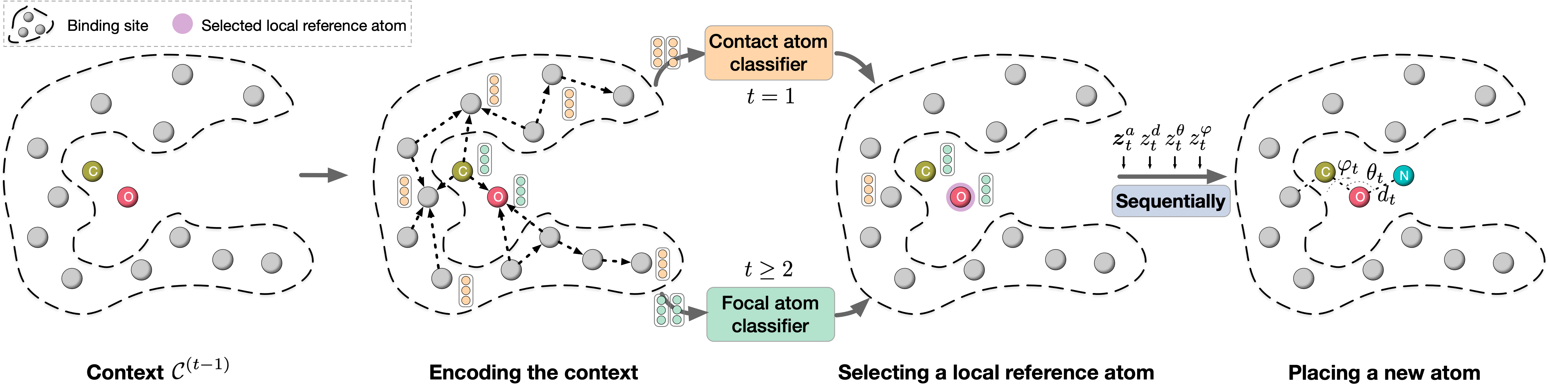
Figure 1: An illustration of one generation step of GraphBP. Details are described in Section 3.1.

3.1 Generation

Overview. In GraphBP, we formulate the generation of 3D molecules in the given binding site as a sequential generation process; that is, we place atoms to the given 3D binding site one by one. At the $t$-th step, we generate the $t$-th atom, including its atom type $\boldsymbol{a}_{t}$ and coordinate $\boldsymbol{r}_{t}$, based on the intermediate contextual information $\mathcal{C}^{(t-1)}$. Note that the context $\mathcal{C}^{(t-1)}$ contains not only the binding site but also the atoms placed in the previous $t-1$ steps, i.e., $\mathcal{C}^{(t-1)}=\mathcal{P}\cup\{(\boldsymbol{a}_{i},\boldsymbol{r}_{i})\}_{i=1}^{t-1}$ when $t\geq 2$. At the first step ($t=1$), the context is the binding site itself, i.e., $\mathcal{C}^{(0)}=\mathcal{P}$.

Within each step, we firstly generate the atom type based on the context. Afterwards, its coordinate is generated by considering both the context and the generated atom type information. Therefore, each step $t\ (t=1,2,\cdots,n)$ of our generation process can be formulated as

$$\boldsymbol{a}_{t}=g^{a}\left(\mathcal{C}^{(t-1)};\boldsymbol{z}_{t}^{a}\right),$$ (3)

$$\boldsymbol{r}_{t}=g^{r}\left(\mathcal{C}^{(t-1)},\boldsymbol{a}_{t};\boldsymbol{z}_{t}^{r}\right),$$

$$\mathcal{C}^{(t)}\leftarrow\mathcal{C}^{(t-1)}\cup\left\{(\boldsymbol{a}_{t},\boldsymbol{r}_{t})\right\}.$$

Generators $g^{a}(\cdot)$ and $g^{r}(\cdot)$ are autoregressive functions. $\boldsymbol{z}_{t}^{a}$ and $\boldsymbol{z}_{t}^{r}$ denote the latent variables used in the flow model at step $t$, which will be introduced in details later.

In the following, we describe the details of one generation step, i.e., how the autoregressive functions $g^{a}(\cdot)$ and $g^{r}(\cdot)$ are parameterized. In addition, we also explain how the key challenges summarized in Section 1 are considered in GraphBP. Particularly, there are mainly three parts in one generation step, namely encoding the context, selecting a local reference atom, and placing a new atom, as illustrated in Figure 1. The details are elucidated as follows.

3.1.1 Encoding the Context

As introduced in Section 1, both geometric shape and chemical interactions are vital to protein-ligand binding affinity. Hence, it is important to capture such information by the context encoder. We firstly construct a graph for the context $\mathcal{C}^{(t-1)}$ by connecting atoms with considering certain cutoff distance. Let $\mathcal{G}^{(t-1)}$ denote the obtained context graph. Afterwards, we employ a 3D graph neural network (3D GNN) to encode $\mathcal{G}^{(t-1)}$. Formally,

$$\{\boldsymbol{h}_{1}^{(t)},\cdots,\boldsymbol{h}_{m+t-1}^{(t)}\}=\text{3DGNN}\left(\mathcal{G}^{(t-1)}\right),$$ (4)

where $\boldsymbol{h}_{k}^{(t)}$ represents the encoded representation of atom $k$ in the context $\mathcal{C}^{(t-1)}$. Note that there are totally $m+t-1$ atoms in the context, including $m$ atoms from the binding site and $t-1$ atoms placed in the previous $t-1$ steps.

The first layer of our 3DGNN is an embedding layer for encoding atom types. Note that we use different learnable embeddings for atoms in the binding site and atoms in the ligand, thereby differentiating ligand atoms from protein atoms. For example, a carbon atom in the ligand and a carbon atom in the protein have different initial representations. Let $\{\boldsymbol{h}_{1}^{(t,0)},\cdots,\boldsymbol{h}_{m+t-1}^{(t,0)}\}$ be the resulting initial representations. Then, we have $L$ feature aggregation layers in our 3DGNN. The aggregation for each atom $k$ at the $\ell$-th layer ($1\leq\ell\leq L$) can be formulated as

$$\boldsymbol{h}_{k}^{(t,\ell)}=\boldsymbol{h}_{k}^{(t,\ell-1)}+\sum_{u\in\mathcal{N}(k)}\boldsymbol{h}_{u}^{(t,\ell-1)}\odot\text{MLP}^{\ell}\left(\boldsymbol{e}_{\text{RBF}}\left(d_{uk}\right)\right),$$ (5)

where $\mathcal{N}(k)$ denotes neighbors of atom $k$ in $\mathcal{G}^{(t-1)}$, $\text{MLP}^{\ell}(\cdot)$ is a multi-layer perceptron, and $\odot$ represents the element-wise multiplication. $\boldsymbol{e}_{\text{RBF}}\left(d_{uk}\right)$ is the high-dimensional embedding of the distance $d_{uk}$ using radial basis functions (RBF), such as Gaussian functions (Schlichtkrull et al., 2018) and spherical Bessel functions (Klicpera et al., 2019). Note that the representations $\{\boldsymbol{h}_{1}^{(t)},\cdots,\boldsymbol{h}_{m+t-1}^{(t)}\}$ obtained by these $L$ feature aggregation layers are invariant to the rotation and translation of the context $\mathcal{C}^{(t-1)}$, since the distance $d_{uk}$ used in Eq. (5) is rotationally and translationally invariant. Our aggregation layer shown in Eq. (5) is a variant of SchNet (Schlichtkrull et al., 2018). We can further employ more advanced but more memory-consuming 3D GNNs (Liu et al., 2021a), such as DimeNet (Klicpera et al., 2019) and SphereNet (Liu et al., 2022), to encode the context information. In this work, we do not use them as our encoder because of insufficient memory budget, given that the context graph could have hundreds of atoms.

3.1.2 Selecting a Local Reference Atom

As described in Section 1, the location of a generated molecule should be equivariant to any rigid transformation of the binding site. In other words, if we rotate or translate the binding site, the generated molecule should be rotated or translated correspondingly. In our sequential generation case, as formulated in Eq. (3), it is desired that the generated coordinate of the $t$-th atom is equivariant to any rigid transformation of the context $\mathcal{C}^{(t-1)}$, while the generated atom type keeps invariant. Formally,

$$g^{a}\left(\mathcal{C}^{(t-1)};\boldsymbol{z}_{t}^{a}\right)=g^{a}\left(\text{RT}\left(\mathcal{C}^{(t-1)}\right);\boldsymbol{z}_{t}^{a}\right),$$ (6)

$$\text{RT}\left(g^{r}\left(\mathcal{C}^{(t-1)},\boldsymbol{a}_{t};\boldsymbol{z}_{t}^{r}\right)\right)=g^{r}\left(\text{RT}\left(\mathcal{C}^{(t-1)}\right),\boldsymbol{a}_{t};\boldsymbol{z}_{t}^{r}\right),$$

where $\text{RT}(\cdot)$ represents any rigid transformation, including rotation, translation, and any composition of them.

As described in Section 3.1.1, our atom representations obtained from context encoding are invariant to any rigid transformation of the context. Thus, it is straightforward to generate invariant atom type by using these representations. Nevertheless, it is non-trivial to generate coordinate that are equivariant to any rigid transformation of the context. To achieve this desirable equivariance, inspired by G-SchNet (Gebauer et al., 2019), MolGym (Simm et al., 2020), and G-SphereNet (Luo & Ji, 2022), we choose to construct a local spherical coordinate system (SCS) and generate the invariant 3-tuple $(d_{t},\theta_{t},\varphi_{t})$ w.r.t. the constructed local SCS.

To construct such local SCS, we consider selecting a local reference atom from the context by using two auxiliary atom-wise classifiers; they are contact atom classifier (for $t=1$) and focal atom classifier (for $t\geq 2$). (i) At the first step ($t=1$), the known context information is the binding site. The contact atom classifier takes the context-encoded representation of each atom in the binding site as input, and determines if the corresponding atom can serve as a local reference atom (i.e., yes or no). The atom selected based on the contact atom classifier will be used as the local reference atom for generating the first atom in the ligand. This selected atom is termed as contact atom because it acts like a “bridge” in contact with the ligand. (ii) For $t\geq 2$, we select a local reference atom from the ligand atoms generated in the previous $t-1$ steps, considering that the new atom is expected to be placed in the local region of the selected reference atom. To be specific, we apply focal atom classifier to the context-encoded representations of all existing atoms in the ligand, which are generated in the previous $t-1$ steps, and classify them into two categories: focal atom and non-focal atom. Then, the selected focal atom will be used as the local reference atom to generate the new atom. Overall, for $t=1$, a local reference atom is selected from the binding site using the contact atom classifier. For $t\geq 2$, a local reference atom is selected from the existing ligand atoms according to the focal atom classifier. We describe how to train these two auxiliary classifiers in Section 3.2.

In general, we need three points in the 3D space to define an SCS. Assuming that the selected local reference atom is the $f$-th atom in the context $\mathcal{C}^{(t-1)}$, we can further find two atoms in the context that are closest and second closest to $f$. These two atoms are denoted as the $c$-th and the $e$-th atom in the context $\mathcal{C}^{(t-1)}$, and they could be in the ligand or in the binding site. With these three atoms $(f,c,e)$, we can construct a local SCS. Further, we can generate the invariant $(d_{t},\theta_{t},\varphi_{t})$ w.r.t. this local SCS. Specifically, $d_{t}$ is distance between the new atom and atom $f$, i.e., $d_{t}=||\boldsymbol{r}_{t}-\boldsymbol{r}_{f}||_{2}$, $\theta_{t}\in[0,\pi]$ is the angle between line $(\boldsymbol{r}_{f},\boldsymbol{r}_{t})$ and line $(\boldsymbol{r}_{f},\boldsymbol{r}_{c})$, and $\varphi_{t}\in[-\pi,\pi]$ is the torsion angle formed by plane $(\boldsymbol{r}_{f},\boldsymbol{r}_{c},\boldsymbol{r}_{t})$ and plane $(\boldsymbol{r}_{f},\boldsymbol{r}_{c},\boldsymbol{r}_{e})$. Afterwards, we can compute $\boldsymbol{r}_{t}$ based on the generated $(d_{t},\theta_{t},\varphi_{t})$ and the known $(\boldsymbol{r}_{f},\boldsymbol{r}_{c},\boldsymbol{r}_{e})$. Note that the constructed local SCS is associated with the context, thus being equivariant to any rigid transformation of the context. In other words, $(\boldsymbol{r}_{f},\boldsymbol{r}_{c},\boldsymbol{r}_{e})$ is equivariant to any rigid transformation of the context. Therefore, the computed $\boldsymbol{r}_{t}$ also keeps equivariant as long as the generated $(d_{t},\theta_{t},\varphi_{t})$ is invariant to any rigid transformation of the context $\mathcal{C}^{(t-1)}$. In addition, we can achieve flexible atom placement since the generated $(d_{t},\theta_{t},\varphi_{t})$ are continuous values, while previous works (Ragoza et al., 2021; Luo et al., 2021a) have to discretize the continuous space during atom placement.

3.1.3 Placing a New Atom

The remaining part in generation is to place a new atom by generating $(d_{t},\theta_{t},\varphi_{t})$ as well as $\boldsymbol{a}_{t}$. As analyzed above, $\boldsymbol{a}_{t}$, $d_{t}$, $\theta_{t}$, and $\varphi_{t}$ should be invariant to any rigid transformation of the context $\mathcal{C}^{(t-1)}$. Hence, it is natural to generate them with context-encoded representations of atoms $(f,c,e)$, i.e., $(\boldsymbol{h}_{f}^{(t)},\boldsymbol{h}_{c}^{(t)},\boldsymbol{h}_{e}^{(t)})$, which are invariant to the rotation and translation of the context $\mathcal{C}^{(t-1)}$. In addition, intuitively, $\boldsymbol{a}_{t}$, $d_{t}$, $\theta_{t}$, and $\varphi_{t}$ are not independent to each other. For example, a carbon atom and an oxygen atom have different distributions over the distance to their local reference atoms. Further, atoms with the same atom type but different distances w.r.t. their local reference atoms could have different distributions over angles. Thus, we propose to generate $\boldsymbol{a}_{t}$, $d_{t}$, $\theta_{t}$, and $\varphi_{t}$ sequentially in each generation step to capture their underlying dependencies. To be specific, we generate these variables using the order $\boldsymbol{a}_{t}\rightarrow d_{t}\rightarrow\theta_{t}\rightarrow\varphi_{t}$, and the generation of each variable is dependent on the previous variables. For instance, to generate $\varphi_{t}$, in addition to $\mathcal{C}^{(t-1)}$, we incorporate the information of $\boldsymbol{a}_{t}$, $d_{t}$, and $\theta_{t}$. Mathematically, $p\left(\boldsymbol{a}_{t},d_{t},\theta_{t},\varphi_{t}|\mathcal{C}^{(t-1)}\right)=p\left(\boldsymbol{a}_{t}|\mathcal{C}^{(t-1)}\right)p\left(d_{t}|\mathcal{C}^{(t-1)}\right)p\left(\theta_{t}|\mathcal{C}^{(t-1)}\right)p\left(\varphi_{t}|\mathcal{C}^{(t-1)}\right)$ does not hold if $\boldsymbol{a}_{t}$, $d_{t}$, $\theta_{t}$, and $\varphi_{t}$ are not independent. In contrast, the following equation always holds according to the multiplication rule of probability, no matter if the variables are independent or not.

$$p\left(\boldsymbol{a}_{t},d_{t},\theta_{t},\varphi_{t}|\mathcal{C}^{(t-1)}\right)=p\left(\boldsymbol{a}_{t}|\mathcal{C}^{(t-1)}\right)p\left(d_{t}|\mathcal{C}^{(t-1)},\boldsymbol{a}_{t}\right)$$ (7)

$$p\left(\theta_{t}|\mathcal{C}^{(t-1)},\boldsymbol{a}_{t},d_{t}\right)p\left(\varphi_{t}|\mathcal{C}^{(t-1)},\boldsymbol{a}_{t},d_{t},\theta_{t}\right).$$

This demonstrates that our generation strategy is also technically sound. We conduct ablation study in Section 4 to demonstrate the effectiveness of this sequential generation strategy. Therefore, our one-step generation, as shown in Eq. (3), can be reformulated as

$$\boldsymbol{a}_{t}=g^{a}\left(\mathcal{C}^{(t-1)};\boldsymbol{z}_{t}^{a}\right),$$ (8)

$$d_{t}=g^{d}\left(\mathcal{C}^{(t-1)},\boldsymbol{a}_{t};z_{t}^{d}\right),$$

$$\theta_{t}=g^{\theta}\left(\mathcal{C}^{(t-1)},\boldsymbol{a}_{t},d_{t};z_{t}^{\theta}\right),$$

$$\varphi_{t}=g^{\varphi}\left(\mathcal{C}^{(t-1)},\boldsymbol{a}_{t},d_{t},\theta_{t};z_{t}^{\varphi}\right),$$

where $\boldsymbol{z}_{t}^{a}\in\mathbb{R}^{p}$, $z_{t}^{d}\in\mathbb{R}$, $z_{t}^{\theta}\in\mathbb{R}$, and $z_{t}^{\varphi}\in\mathbb{R}$ are all latent variables used in the flow model. During generation, we sample latent variables from known prior Gaussian distributions, and then map them to variables of interest (i.e., $\boldsymbol{a}_{t}$, $d_{t}$, $\theta_{t}$, $\varphi_{t}$). For training, we map observed variables to latent variables, and maximize their likelihood. Since the atom type vector is discrete, which cannot fit into a flow model, we convert it to a continuous variable during training using dequantization techniques (Kingma & Dhariwal, 2018). This is widely used by existing molecule generation methods (Madhawa et al., 2019; Shi et al., 2019; Liu et al., 2021b). Specifically, we add uniform noise as $\boldsymbol{\tilde{a}}_{t}=\boldsymbol{a}_{t}+\boldsymbol{u}$, $\boldsymbol{u}\sim\mathcal{U}(0,1)^{p}$. In the following, we elaborate how to employ flow model to construct invertible mappings $\boldsymbol{z}_{t}^{a}\rightarrow\boldsymbol{\tilde{a}}_{t}$, $z_{t}^{d}\rightarrow d_{t}$, $z_{t}^{\theta}\rightarrow\theta_{t}$, and $z_{t}^{\varphi}\rightarrow\varphi_{t}$, respectively. The training scheme is elucidated in Section 3.2.

To generate $\boldsymbol{a}_{t}$, we first apply affine transformation to map the latent variable $\boldsymbol{z}_{t}^{a}$ to $\boldsymbol{\tilde{a}}_{t}$. Formally,

$$\boldsymbol{\tilde{a}}_{t}=\boldsymbol{\sigma}_{t}^{a}\left(\mathcal{C}^{(t-1)}\right)\odot\boldsymbol{z}_{t}^{a}+\boldsymbol{\mu}_{t}^{a}\left(\mathcal{C}^{(t-1)}\right),$$ (9)

where the scale factor $\boldsymbol{\sigma}_{t}^{a}(\cdot)\in\mathbb{R}^{p}$ and the translation factor $\boldsymbol{\mu}_{t}^{a}(\cdot)\in\mathbb{R}^{p}$ are both dependent on the context $\mathcal{C}^{(t-1)}$. To be specific, they are computed by applying MLPs to the context-encoded representation of the selected local reference atom $f$. Formally,

$$\begin{cases}\begin{aligned} \boldsymbol{\sigma}_{t}^{a}\left(\mathcal{C}^{(t-1)}\right)&=\text{MLP}_{\sigma}^{a}\left(\boldsymbol{h}_{f}^{(t)}\right),\\ \boldsymbol{\mu}_{t}^{a}\left(\mathcal{C}^{(t-1)}\right)&=\text{MLP}_{\mu}^{a}\left(\boldsymbol{h}_{f}^{(t)}\right).\\ \end{aligned}\end{cases}$$ (10)

After obtaining $\boldsymbol{\tilde{a}}_{t}$, we can derive the one-hot $\boldsymbol{a}_{t}$ by performing the argmax operation to $\boldsymbol{\tilde{a}}_{t}$.

Similar to the generation of atom type, we can produce $d_{t}$, $\theta_{t}$, and $\varphi_{t}$ as

$$d_{t} =\sigma_{t}^{d}\left(\mathcal{C}^{(t-1)},\boldsymbol{a}_{t}\right)\odot z_{t}^{d}+\mu_{t}^{d}\left(\mathcal{C}^{(t-1)},\boldsymbol{a}_{t}\right),$$ (11)

$$\theta_{t} =\sigma_{t}^{\theta}\left(\mathcal{C}^{(t-1)},\boldsymbol{a}_{t},d_{t}\right)\odot z_{t}^{\theta}+\mu_{t}^{\theta}\left(\mathcal{C}^{(t-1)},\boldsymbol{a}_{t},d_{t}\right),$$

$$\varphi_{t} =\sigma_{t}^{\varphi}\left(\mathcal{C}^{(t-1)},\boldsymbol{a}_{t},d_{t},\theta_{t}\right)\odot z_{t}^{\varphi}+\mu_{t}^{\varphi}\left(\mathcal{C}^{(t-1)},\boldsymbol{a}_{t},d_{t},\theta_{t}\right).$$

The scale factors $\sigma_{t}^{d}(\cdot),\sigma_{t}^{\theta}(\cdot),\sigma_{t}^{\varphi}(\cdot)\in\mathbb{R}$ and the translation factors $\mu_{t}^{d}(\cdot),\mu_{t}^{\theta}(\cdot),\mu_{t}^{\varphi}(\cdot)\in\mathbb{R}$ are dependent on their corresponding conditional information that are defined and justified in our generation strategy, as formulated in Eq. (8). These factors are also naturally parameterized by MLPs with considering their respective conditional information. To be specific,

$$\boldsymbol{h}_{f/c/e}^{(t)^{\prime}}=\boldsymbol{h}_{f/c/e}^{(t)}\odot\text{Embedding}\left(\boldsymbol{a}_{t}\right),$$ (12)

$$\begin{cases}\begin{aligned} \sigma_{t}^{d}\left(\mathcal{C}^{(t-1)},\boldsymbol{a}_{t}\right)&=\text{MLP}_{\sigma}^{d}\left(\boldsymbol{h}_{f}^{(t)^{\prime}}\right),\\ \mu_{t}^{d}\left(\mathcal{C}^{(t-1)},\boldsymbol{a}_{t}\right)&=\text{MLP}_{\mu}^{d}\left(\boldsymbol{h}_{f}^{(t)^{\prime}}\right),\end{aligned}\end{cases}$$ (13)

$$\boldsymbol{h}_{f/c/e}^{(t)^{\prime\prime}}=\boldsymbol{h}_{f/c/e}^{(t)^{\prime}}\odot\text{LB}_{\text{RBF}}\left(\boldsymbol{e}_{\text{RBF}}\left(d_{t}\right)\right),$$ (14)

$$\begin{cases}\begin{aligned} \sigma_{t}^{\theta}\left(\mathcal{C}^{(t-1)},\boldsymbol{a}_{t},d_{t}\right)&=\text{MLP}_{\sigma}^{\theta}\left(\left[\boldsymbol{h}_{f}^{(t)^{\prime\prime}},\boldsymbol{h}_{c}^{(t)^{\prime\prime}}\right]\right),\\ \mu_{t}^{\theta}\left(\mathcal{C}^{(t-1)},\boldsymbol{a}_{t},d_{t}\right)&=\text{MLP}_{\mu}^{\theta}\left(\left[\boldsymbol{h}_{f}^{(t)^{\prime\prime}},\boldsymbol{h}_{c}^{(t)^{\prime\prime}}\right]\right),\end{aligned}\end{cases}$$ (15)

$$\boldsymbol{h}_{f/c/e}^{(t)^{\prime\prime\prime}}=\boldsymbol{h}_{f/c/e}^{(t)^{\prime\prime}}\odot\text{LB}_{\text{CBF}}\left(\boldsymbol{e}_{\text{CBF}}\left(d_{t},\theta_{t}\right)\right),$$ (16)

$$\begin{cases}\begin{aligned} \sigma_{t}^{\varphi}\left(\mathcal{C}^{(t-1)},\boldsymbol{a}_{t},d_{t},\theta_{t}\right)&=\text{MLP}_{\sigma}^{\varphi}\left(\left[\boldsymbol{h}_{f}^{(t)^{\prime\prime\prime}},\boldsymbol{h}_{c}^{(t)^{\prime\prime\prime}},\boldsymbol{h}_{e}^{(t)^{\prime\prime\prime}}\right]\right),\\ \mu_{t}^{\varphi}\left(\mathcal{C}^{(t-1)},\boldsymbol{a}_{t},d_{t},\theta_{t}\right)&=\text{MLP}_{\mu}^{\varphi}\left(\left[\boldsymbol{h}_{f}^{(t)^{\prime\prime\prime}},\boldsymbol{h}_{c}^{(t)^{\prime\prime\prime}},\boldsymbol{h}_{e}^{(t)^{\prime\prime\prime}}\right]\right).\end{aligned}\end{cases}$$ (17)

$\text{Embedding}\left(\cdot\right)$ is the same embedding layer that is used to encode ligand atom types during context encoding. Multiplying the embedding of $\boldsymbol{a}_{t}$ in Eq. (12) helps to incorporate the generated atom type information in the subsequent generation for $d_{t}$, $\theta_{t}$, and $\varphi_{t}$. As the distance embedding in Eq. (5), $\boldsymbol{e}_{\text{RBF}}\left(d_{t}\right)$ is the RBF embedding of the distance $d_{t}$. Further, $\boldsymbol{e}_{\text{CBF}}\left(d_{t},\theta_{t}\right)$ denotes the high-dimensional embedding of $(d_{t},\theta_{t})$ with circular basis functions (CBF). We use the same circular basis functions as previous works that consider geometric information (Klicpera et al., 2019; Liu et al., 2022; Klicpera et al., 2021). $\text{LB}_{\text{RBF/CBF}}(\cdot)$ represents a linear layer and $[\cdot]$ denotes the concatenation operation. Intuitively, incorporating the distance embedding in Eq. (14) and distance-angle embedding in Eq. (16) can guide the subsequent generation for $\theta_{t}$ and $\varphi_{t}$, respectively. This aims to capture the underlying dependencies of variables $\boldsymbol{a}_{t}$, $d_{t}$, $\theta_{t}$, and $\varphi_{t}$.

3.1.4 Overall Generation Process

So far, we have described the key components of our generative framework. To generate a 3D molecular geometry for a given binding site, we autoregressively place one atom at each step. At each step $t$, we firstly encode the current known context information, then select a local reference atom with our auxiliary classifiers, and finally place a new atom by producing $\boldsymbol{a}_{t}$, $d_{t}$, $\theta_{t}$, and $\varphi_{t}$ sequentially. We illustrate one generation step of our GraphBP in Figure 1. The autoregressive generation will be terminated if either no atom in the ligand can serve as a local reference atom according to the focal atom classifier or a predefined maximum number of atoms has been achieved. Afterwards, following previous works (Ragoza et al., 2021; Luo et al., 2021a), we apply OpenBabel (O’Boyle et al., 2011) to construct bonds based on our generated 3D molecular geometries.

3.2 Training

To train our autoregressive generative model, we need to decompose a 3D molecule in a ligand-protein pair to a trajectory of atom placement steps. Inspired by G-SphereNet (Luo & Ji, 2022), we expect that the new atom should be placed in the local region of the reference atom during generation. Thus, we select the atom in the binding site that is closest to the ligand as the first local reference atom, i.e., contact atom, and the atom in the ligand that is closest to the binding site as the first atom to be generated. Then, starting from this selected atom in the ligand, we apply Prim’s algorithm on the 3D molecular geometry to obtain the placement order of atoms in the ligand, as well as their corresponding local reference atoms. This strategy can guarantee that the new atom for each step is always in the local region of the corresponding reference atom. With such obtained trajectory, GraphBP is trained by stochastic gradient descent using the following three loss functions.

Atom placement loss $\mathcal{L}_{ap}$. As described in Eq. (1), with flow model, we can compute the log-likelihood of training data and maximize it. Hence, the training loss function for atom placement is defined as the negative of the computed log-likelihood of the training trajectory. Formally, for a 3D molecular geometry with $n$ atoms, we have

$$\mathcal{L}_{ap}= -\sum_{t=1}^{n}\left[\left(\log\left(\text{PD}\left(p_{Z_{a}}\left(\boldsymbol{z}_{t}^{a}\right)\right)\right)+\log\left(\left|\text{PD}\left(\frac{1}{\boldsymbol{\sigma}_{t}^{a}}\right)\right|\right)\right)\right.$$ (18)

$$+\left(\log\left(p_{Z_{d}}\left(z_{t}^{d}\right)\right)+\log\left(\left|\frac{1}{\sigma_{t}^{d}}\right|\right)\right)$$

$$+\left(\log\left(p_{Z_{\theta}}\left(z_{t}^{\theta}\right)\right)+\log\left(\left|\frac{1}{\sigma_{t}^{\theta}}\right|\right)\right)$$

$$\left.+\left(\log\left(p_{Z_{\varphi}}\left(z_{t}^{\varphi}\right)\right)+\log\left(\left|\frac{1}{\sigma_{t}^{\varphi}}\right|\right)\right)\right].$$

$\text{PD}(\cdot)$ is used to represent the product of elements across dimensions of a vector, since $\boldsymbol{z}_{t}^{a}$ and $\boldsymbol{\sigma}_{t}^{a}$ are both $p$-dimensional vectors. Latent variables $\boldsymbol{z}_{t}^{a}$, $z_{t}^{d}$, $z_{t}^{\theta}$ and $z_{t}^{\varphi}$ can be computed by the inverted mappings of Eq. (9) and Eq. (11), such as $z_{t}^{d}=\frac{d_{t}-\mu_{t}^{d}}{\sigma_{t}^{d}}$. $p_{Z_{a}}$, $p_{Z_{d}}$, $p_{Z_{\theta}}$, and $p_{Z_{\varphi}}$ are prior Gaussian distributions. The detailed derivation of $\mathcal{L}_{ap}$ is included in Appendix A.

Contact atom classifier loss $\mathcal{L}_{cc}$. The contact atom classifier is used to select the first local reference atom from the binding site. We train it with the standard binary cross entropy loss. In particular, we use the contact atom, which is the atom in the binding site that is closest to the ligand, as the positive sample, and the atom in the binding site that is furthest to the ligand, as the negative sample.

Focal atom classifier loss $\mathcal{L}_{fc}$. The focal atom classifier is also trained with the standard binary cross entropy loss and used for selecting a local reference atom from the existing ligand atoms. The ground truth for an atom is negative if all of its bonded atoms have been generated, otherwise positive.

In summary, the overall loss function for training GraphBP is $\mathcal{L}=\mathcal{L}_{ap}+\mathcal{L}_{cc}+\mathcal{L}_{fc}$.

4 Experiments

We firstly evaluate the ability of our GraphBP to generate 3D molecules that are capable of binding to given protein targets. The experiment demonstrates that GraphBP outperforms baselines by significant margins. Afterwards, we perform ablation studies to verify the effectiveness of the sequential generation proposed in Section 3.1.3.

Dataset. We use the CrossDocked2020 dataset (Francoeur et al., 2020), which contains over $22$ million docked protein-ligand crystal structures, to evaluate GraphBP for structure-based drug design. Following LiGAN (Ragoza et al., 2021), we ignore any poses that have root-mean-squared deviations (RMSD) greater than $2$Å, thus obtaining a dataset with around $500$k protein-ligand complexes. We use the same training set and test set, as used in LiGAN, for fair comparison. Total number of atom types in ligands and in binding sites are $27$ and $19$, respectively. The atom types are summarized in Appendix B.

Setup. We use the same $10$ target proteins as LiGAN for test evaluation. Each of them could have multiple associated ligands, leading to $90$ protein-ligand pairs in the test set as reference. Following LiGAN, we generate $100$ molecules with GraphBP for each reference binding site in the test set. This evaluation setting is challenging because the test targets are diversely selected from different pocket clusters and the reference ligand usually bind strongly to the target binding site (Ragoza et al., 2021). We quantitatively measure the generation performance by two metrics: (i) Validity is the percentage of chemically valid molecules among all generated molecules. A molecule is valid if it can be sanitized by RDkit (Landrum et al., 2006). (ii) $\Delta$Binding measures the percentage of generated molecules that have higher predicted binding affinity than their corresponding reference molecules. Note that we are unable to perform wet-lab experiment assays to evaluate the binding affinity of generated molecules. Also, there does not exist a computational metric that can serve as a golden standard for assessing binding affinity. Hence, following LiGAN, the binding affinity is predicted by an ensemble of CNN scoring functions (Ragoza et al., 2017) that were trained on the CrossDocked2020 data set. Such CNN predicted affinity has been shown to be more accurate than using the Autodock Vina empirical scoring function (Trott & Olson, 2010). Therefore, it can be used as a reasonable and convincing metric for evaluating the binding affinity of generated molecules. Following LiGAN, we firstly refine the generated 3D molecules by Universal Force Field minimization (Rappé et al., 1992). Afterwards, Vina minimization and CNN scoring are applied to both generated and reference molecules by using gnina, a molecular docking program (McNutt et al., 2021).

Baselines. We consider two variants from the recent LiGAN (Ragoza et al., 2021) method as baselines. LiGAN-prior generates molecules conditional on the given binding sites, which has the identical conditional information as our GraphBP. LiGAN-posterior encodes the whole reference protein-ligand complex as conditional information, thus generating molecules biased towards the reference molecule. Note that LiGAN-posterior incorporates more conditional information than GraphBP and LiGAN-prior.

Table 1: Generation performance on structure-based drug design. $\uparrow$ represents that higher value indicates better performance.

Method	Validity↑	$\Delta$Binding↑
LiGAN-prior	90.9%	15.9%
LiGAN-posterior	98.5%	15.4%
GraphBP (ours)	99.7%	27.0%

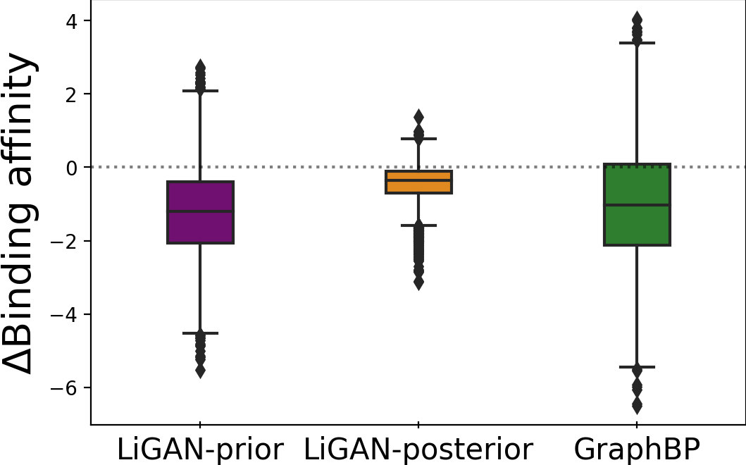
Figure 2: Visualization of $\Delta$Binding affinity distributions for LiGAN and GraphBP. The values denote the relative improvements of generated molecules over their corresponding reference molecules.

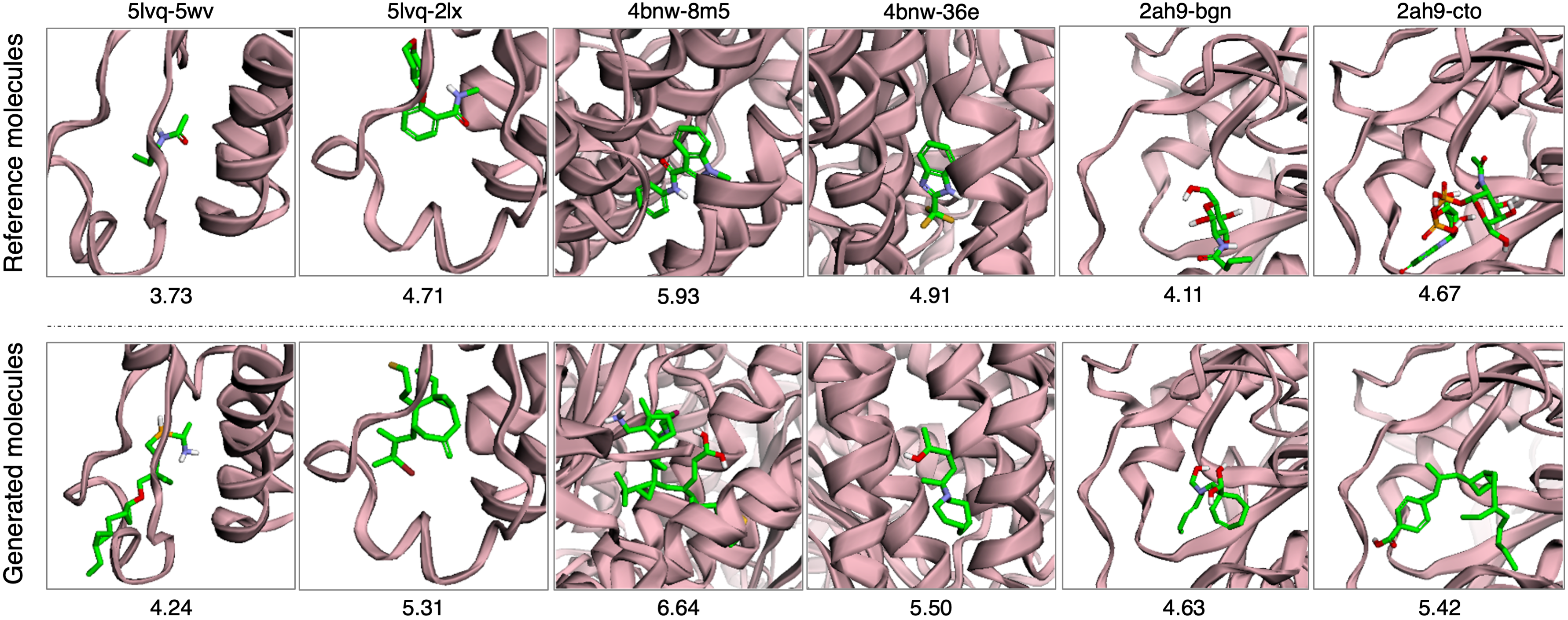
Figure 3: Several examples of generated 3D molecules that have higher predicted binding affinity than reference molecules. The PDB IDs and the ligand IDs of proteins and reference molecules are labeled on the top.

Table 2: Comparison on random molecular geometry generation task between our method and ablation models. $\uparrow$ ($\downarrow$) represents that higher (lower) value indicates better performance. The top two results in terms of each metric are highlighted as 1st and 2nd.

Method	Validity↑	MMD distances↓
		C-C	C-N	C-O	H-C	H-N	H-O	Avg.
No dep.	25.35%	0.776	0.499	1.251	2.600	0.823	2.849	1.466
Partial dep.	76.72%	0.343	0.384	0.257	0.227	0.373	0.828	0.402
Ours	81.98%	0.232	0.160	0.475	0.058	0.318	0.202	0.241

Results. We present the quantitative results in Table 1. Our GraphBP can generate more valid molecules than baselines, including LiGAN-posterior which even includes a valid reference ligand as conditional information. More importantly, $27.0\%$ of molecules generated by GraphBP have higher predicted binding affinity than reference molecules. This outperforms LiGAN by an absolute margin of $11.1\%$. These significant improvements over baselines demonstrate that GraphBP, which incorporates graph representations and a more flexible atom placement strategy, can capture the underlying distribution of 3D molecular geometries conditional on binding sites more effectively.

We further provide the detailed distributions of $\Delta$Binding affinity in Figure 2. Note that LiGAN-posterior achieves higher average $\Delta$Binding affinity but lower variance than LiGAN-prior and GraphBP. This indicates that LiGAN-posterior, with encoding the reference molecules as conditions, might perform slight modifications on reference molecules. Even though, compared with LiGAN-posterior, our GraphBP still generates more molecules that are predicted to bind more strongly than reference molecules ($27.0\%$ vs. $15.4\%$), demonstrating that GraphBP can generate more diverse molecules to bind with target proteins by effectively capturing the underlying conditional distribution.

In Figure 3, we provide several examples of generated 3D molecules that are predicted to bind more strongly to the target proteins than their corresponding reference molecules. It can be observed that our generated molecules with higher predicted binding affinity are largely different from reference molecules, further indicating that our model is capable of generating diverse and novel molecules to bind target proteins, instead of simply memorizing or modifying known molecules.

Ablation studies. In Section 3.1.3, we propose to generate the variables of interest sequentially to capture their underlying dependencies. Specifically, given context $\mathcal{C}^{(t-1)}$, we produce $\boldsymbol{a}_{t}$, $d_{t}$, $\theta_{t}$, and $\varphi_{t}$ one by one as $\mathcal{C}^{(t-1)}\rightarrow\boldsymbol{a}_{t}\rightarrow d_{t}\rightarrow\theta_{t}\rightarrow\varphi_{t}$. To verify the effectiveness of this strategy, we employ the following two variants. (i) No dependencies. The variables $\boldsymbol{a}_{t}$, $d_{t}$, $\theta_{t}$, and $\varphi_{t}$ are generated independently from the context, as $\mathcal{C}^{(t-1)}\rightarrow\boldsymbol{a}_{t}$, $\mathcal{C}^{(t-1)}\rightarrow d_{t}$, $\mathcal{C}^{(t-1)}\rightarrow\theta_{t}$, and $\mathcal{C}^{(t-1)}\rightarrow\varphi_{t}$. Thus, we omit the incorporating of atom type embedding (Eq. (12)), distance embedding (Eq. (14)), and distance-angle embedding (Eq. (16)). (ii) Partial dependencies. We consider the generated atom type information when generating $d_{t}$, $\theta_{t}$, and $\varphi_{t}$. However, $d_{t}$, $\theta_{t}$, and $\varphi_{t}$ are treated independently. It can be denoted as $\mathcal{C}^{(t-1)}\rightarrow\boldsymbol{a}_{t}$, $(\mathcal{C}^{(t-1)},\boldsymbol{a}_{t})\rightarrow d_{t}$, $(\mathcal{C}^{(t-1)},\boldsymbol{a}_{t})\rightarrow\theta_{t}$, and $(\mathcal{C}^{(t-1)},\boldsymbol{a}_{t})\rightarrow\varphi_{t}$, leading to a similar model as G-SphereNet (Luo & Ji, 2022). For efficiency, we choose to conduct experiments on random molecular geometry generation, avoiding encoding large binding sites. Following G-SphereNet, we train models on 3D molecules from QM9 (Ramakrishnan et al., 2014) and evaluate the generated molecular geometries. The evaluation metrics are validity of generated molecules and the Maximum Mean Discrepancy (MMD) (Gretton et al., 2012) distances of bond length distributions between generated 3D molecules and training 3D molecules. The bond length distributions of molecules generated by different models and training molecules are illustrated in Figure 5, Appendix C.

The comparison is summarized in Table 2. It shows that adding dependencies improves the generation performance consistently. Our sequential generation method performs best, demonstrating that it can model the distribution of molecular geometries more effectively by capturing the underlying dependencies among the variables. Since the loss for atom placement (Eq. (18)) can be divided into losses w.r.t. atom type, distance, angle, and torsion, respectively, we can further analyze the modeling ability for these variables by observing their corresponding training losses. We illustrate the comparison of training losses in Figure 4. By observing the loss for each variable, we can conclude that adding dependencies can help to fit the training data better.

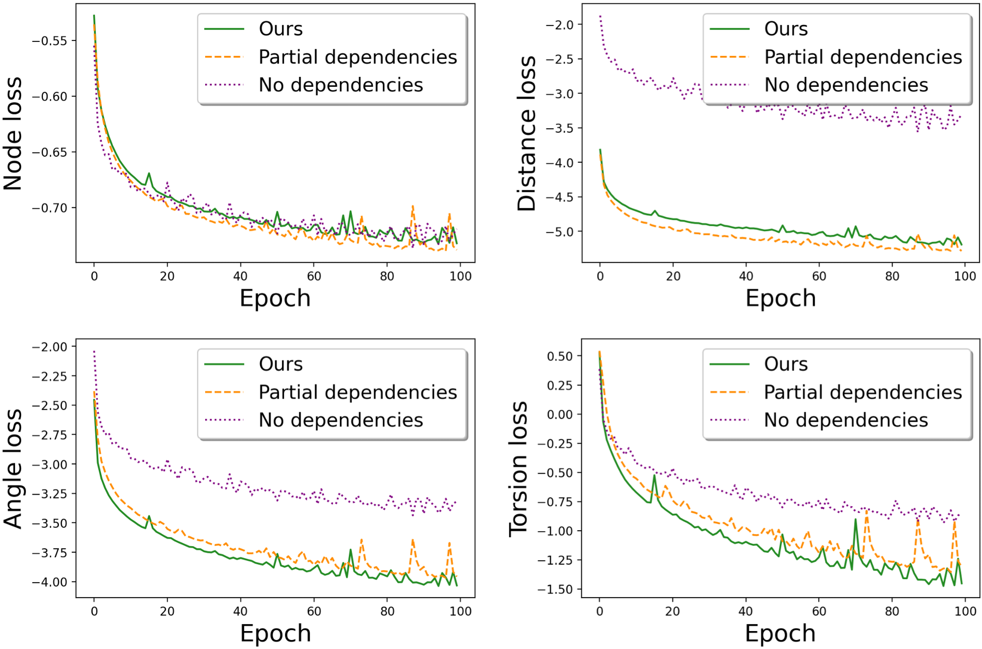
Figure 4: Comparison of training losses between our method and ablation models.

5 Conclusions

In this work, we propose GraphBP, a machine learning approach to generate 3D molecules for target protein binding. GraphBP is capable of capturing 3D geometric structures and chemical interactions of protein-ligand complexes, placing atoms without discretizing the 3D space, and preserving the equivariance property during generation. GraphBP is shown to be effective and outperforms recent baselines significantly in generating 3D molecules that bind strongly to target proteins.

Appendix A The Detailed Derivation of $\mathcal{L}_{ap}$

The detailed derivation of $\mathcal{L}_{ap}$, as introduced in Eq. (18), is as follows.

$$\mathcal{L}_{ap} =-\log\prod_{t=1}^{n}p\left(\boldsymbol{a}_{t},d_{t},\theta_{t},\varphi_{t}|\mathcal{C}^{(t-1)}\right)$$ (19)

$$=-\sum_{t=1}^{n}\log p\left(\boldsymbol{a}_{t},d_{t},\theta_{t},\varphi_{t}|\mathcal{C}^{(t-1)}\right)$$ (20)

$$=-\sum_{t=1}^{n}\log p\left(\boldsymbol{a}_{t}|\mathcal{C}^{(t-1)}\right)p\left(d_{t}|\mathcal{C}^{(t-1)},\boldsymbol{a}_{t}\right)p\left(\theta_{t}|\mathcal{C}^{(t-1)},\boldsymbol{a}_{t},d_{t}\right)p\left(\varphi_{t}|\mathcal{C}^{(t-1)},\boldsymbol{a}_{t},d_{t},\theta_{t}\right)$$ (21)

$$=-\sum_{t=1}^{n}\left(\log p\left(\boldsymbol{a}_{t}|\mathcal{C}^{(t-1)}\right)+\log p\left(d_{t}|\mathcal{C}^{(t-1)},\boldsymbol{a}_{t}\right)+\log p\left(\theta_{t}|\mathcal{C}^{(t-1)},\boldsymbol{a}_{t},d_{t}\right)+\log p\left(\varphi_{t}|\mathcal{C}^{(t-1)},\boldsymbol{a}_{t},d_{t},\theta_{t}\right)\right)$$ (22)

$$\triangleq-\sum_{t=1}^{n}\left(\log p\left(\boldsymbol{\tilde{a}}_{t}|\mathcal{C}^{(t-1)}\right)+\log p\left(d_{t}|\mathcal{C}^{(t-1)},\boldsymbol{a}_{t}\right)+\log p\left(\theta_{t}|\mathcal{C}^{(t-1)},\boldsymbol{a}_{t},d_{t}\right)+\log p\left(\varphi_{t}|\mathcal{C}^{(t-1)},\boldsymbol{a}_{t},d_{t},\theta_{t}\right)\right)$$ (23)

$$\begin{split}=-\sum_{t=1}^{n}\left[\left(\log\left(\text{PD}\left(p_{Z_{a}}\left(\boldsymbol{z}_{t}^{a}\right)\right)\right)+\log\left(\left|\text{PD}\left(\frac{1}{\boldsymbol{\sigma}_{t}^{a}}\right)\right|\right)\right)+\left(\log\left(p_{Z_{d}}\left(z_{t}^{d}\right)\right)+\log\left(\left|\frac{1}{\sigma_{t}^{d}}\right|\right)\right)\right.\\ \left.+\left(\log\left(p_{Z_{\theta}}\left(z_{t}^{\theta}\right)\right)+\log\left(\left|\frac{1}{\sigma_{t}^{\theta}}\right|\right)\right)+\left(\log\left(p_{Z_{\varphi}}\left(z_{t}^{\varphi}\right)\right)+\log\left(\left|\frac{1}{\sigma_{t}^{\varphi}}\right|\right)\right)\right].\end{split}$$ (24)

$\text{PD}(\cdot)$ is used to represent the product of elements across dimensions of a vector, since $\boldsymbol{z}_{t}^{a}$ and $\boldsymbol{\sigma}_{t}^{a}$ are both $p$-dimensional vectors. Eq. (24) is obtained from Eq. (23) by the property of autoregressive flow models, as described in Eq. (1). Latent variables $\boldsymbol{z}_{t}^{a}$, $z_{t}^{d}$, $z_{t}^{\theta}$ and $z_{t}^{\varphi}$ can be computed by the inverted mappings of Eq. (9) and Eq. (11), such as $z_{t}^{d}=\frac{d_{t}-\mu_{t}^{d}}{\sigma_{t}^{d}}$. $p_{Z_{a}}$, $p_{Z_{d}}$, $p_{Z_{\theta}}$, and $p_{Z_{\varphi}}$ are prior Gaussian distributions.

Since we apply dequantization technique to obtain $\boldsymbol{\tilde{a}}_{t}$ from $\boldsymbol{a}_{t}$ during training, the first term in Eq. (23) maximizes the log-likelihood of $p\left(\boldsymbol{\tilde{a}}_{t}|\mathcal{C}^{(t-1)}\right)$ instead of $p\left(\boldsymbol{a}_{t}|\mathcal{C}^{(t-1)}\right)$. We have to use this dequantization technique since flow model used in our framework does not apply to discrete data directly. Note that we can simply perform argmax operation to convert $\boldsymbol{\tilde{a}}_{t}$ back to $\boldsymbol{a}_{t}$. Hence, such dequantization can be viewed as an operation similar to data augmentation during training. Such dequantization technique is widely used and shown to be effective by existing molecule generation methods (Madhawa et al., 2019; Shi et al., 2019; Liu et al., 2021b).

Appendix B Dataset Details

There are totally $27$ atom types for ligands; they are B, C, N, O, F, Mg, Al, Si, P, S, Cl, Sc, V, Fe, Cu, Zn, As, Se, Br, Y, Mo, Ru, Rh, Sb, I, W, and Au. For binding sites, there are $19$ possible atom types, including C, N, O, Na, Mg, P, S, Cl, K, Ca, Mn, Co, Cu, Zn, Se, Cd, I, Cs, and Hg.

Appendix C More Experimental Results

The bond length distributions of molecules generated by different models and training molecules are compared in Figure 5. We can observe that adding dependencies among variables helps to improve the modeling ability. Our sequential generation strategy outperforms ablation variants consistently.

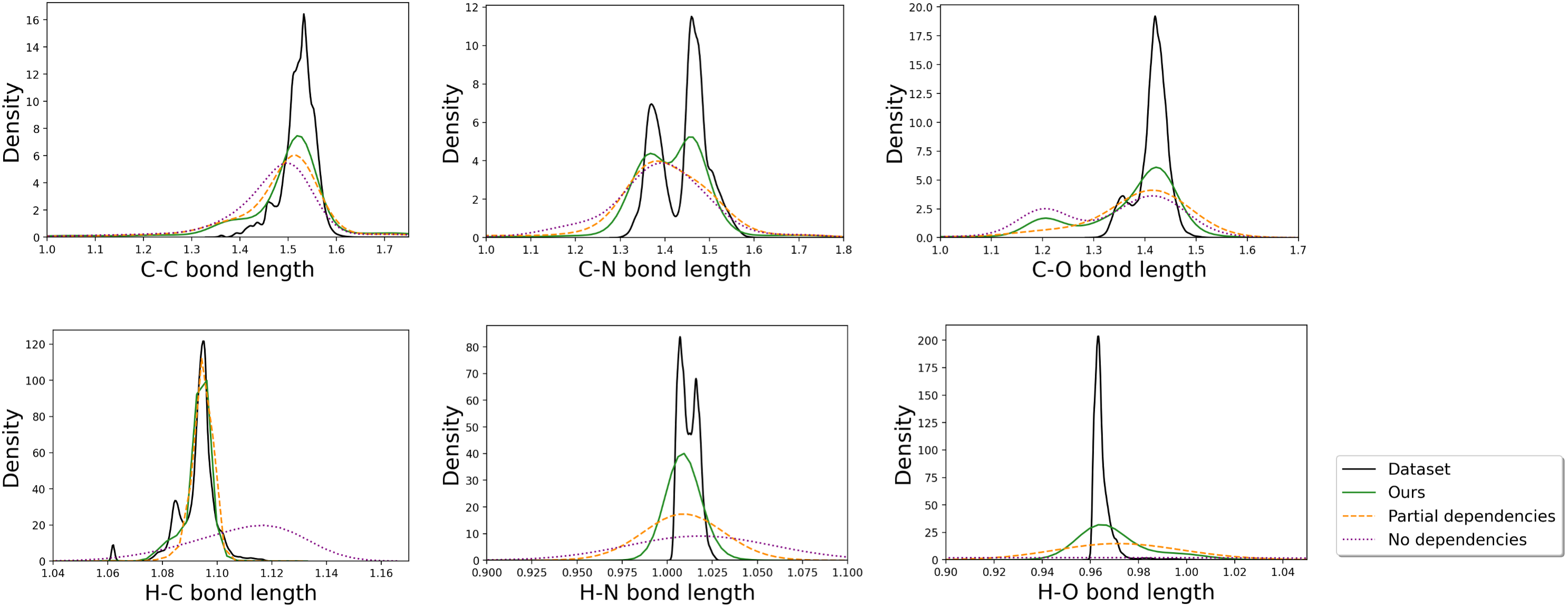
Figure 5: Visualization of bond length distributions of generated molecules and training molecules.

References

- Anderson (2003) Anderson, A. C. The process of structure-based drug design. Chemistry & biology, 10(9):787–797, 2003.
- Dai et al. (2018) Dai, H., Tian, Y., Dai, B., Skiena, S., and Song, L. Syntax-directed variational autoencoder for structured data. In International Conference on Learning Representations, 2018.
- De Cao & Kipf (2018) De Cao, N. and Kipf, T. MolGAN: An implicit generative model for small molecular graphs. arXiv preprint arXiv:1805.11973, 2018.
- Dinh et al. (2014) Dinh, L., Krueger, D., and Bengio, Y. Nice: Non-linear independent components estimation. arXiv preprint arXiv:1410.8516, 2014.
- Du et al. (2022) Du, Y., Fu, T., Sun, J., and Liu, S. MolGenSurvey: A systematic survey in machine learning models for molecule design. arXiv preprint arXiv:2203.14500, 2022.
- Francoeur et al. (2020) Francoeur, P. G., Masuda, T., Sunseri, J., Jia, A., Iovanisci, R. B., Snyder, I., and Koes, D. R. Three-dimensional convolutional neural networks and a cross-docked data set for structure-based drug design. Journal of Chemical Information and Modeling, 60(9):4200–4215, 2020.
- Ganea et al. (2021) Ganea, O.-E., Pattanaik, L., Coley, C. W., Barzilay, R., Jensen, K. F., Green, W. H., and Jaakkola, T. S. GeoMol: Torsional geometric generation of molecular 3d conformer ensembles. Advances in Neural Information Processing Systems, 2021.
- Gebauer et al. (2019) Gebauer, N. W., Gastegger, M., and Schütt, K. T. Symmetry-adapted generation of 3d point sets for the targeted discovery of molecules. In Proceedings of the 33rd International Conference on Neural Information Processing Systems, pp. 7566–7578, 2019.
- Gogineni et al. (2020) Gogineni, T., Xu, Z., Punzalan, E., Jiang, R., Kammeraad, J., Tewari, A., and Zimmerman, P. TorsionNet: A reinforcement learning approach to sequential conformer search. Advances in Neural Information Processing Systems, 33:20142–20153, 2020.
- Gómez-Bombarelli et al. (2018) Gómez-Bombarelli, R., Wei, J. N., Duvenaud, D., Hernández-Lobato, J. M., Sánchez-Lengeling, B., Sheberla, D., Aguilera-Iparraguirre, J., Hirzel, T. D., Adams, R. P., and Aspuru-Guzik, A. Automatic chemical design using a data-driven continuous representation of molecules. ACS central science, 4(2):268–276, 2018.
- Goodfellow et al. (2014) Goodfellow, I., Pouget-Abadie, J., Mirza, M., Xu, B., Warde-Farley, D., Ozair, S., Courville, A., and Bengio, Y. Generative adversarial nets. Advances in neural information processing systems, 27:2672–2680, 2014.
- Gretton et al. (2012) Gretton, A., Borgwardt, K. M., Rasch, M. J., Schölkopf, B., and Smola, A. A kernel two-sample test. The Journal of Machine Learning Research, 13(1):723–773, 2012.
- Hoffmann & Noé (2019) Hoffmann, M. and Noé, F. Generating valid euclidean distance matrices. arXiv preprint arXiv:1910.03131, 2019.
- Ji et al. (2012) Ji, S., Xu, W., Yang, M., and Yu, K. 3d convolutional neural networks for human action recognition. IEEE transactions on pattern analysis and machine intelligence, 35(1):221–231, 2012.
- Jin et al. (2018) Jin, W., Barzilay, R., and Jaakkola, T. Junction tree variational autoencoder for molecular graph generation. In International Conference on Machine Learning, pp. 2323–2332, 2018.
- Jumper et al. (2021) Jumper, J., Evans, R., Pritzel, A., Green, T., Figurnov, M., Ronneberger, O., Tunyasuvunakool, K., Bates, R., Žídek, A., Potapenko, A., et al. Highly accurate protein structure prediction with alphafold. Nature, 596(7873):583–589, 2021.
- Kingma & Dhariwal (2018) Kingma, D. P. and Dhariwal, P. Glow: Generative flow with invertible 1x1 convolutions. In Advances in neural information processing systems, pp. 10215–10224, 2018.
- Kingma & Welling (2013) Kingma, D. P. and Welling, M. Auto-encoding variational bayes. arXiv preprint arXiv:1312.6114, 2013.
- Klicpera et al. (2019) Klicpera, J., Groß, J., and Günnemann, S. Directional message passing for molecular graphs. In International Conference on Learning Representations, 2019.
- Klicpera et al. (2021) Klicpera, J., Becker, F., and Günnemann, S. Gemnet: Universal directional graph neural networks for molecules. In Conference on Neural Information Processing Systems (NeurIPS), 2021.
- Kusner et al. (2017) Kusner, M., Paige, B., and Hernández-Lobato, J. Grammar variational autoencoder. In Proceedings of the 34 th International Conference on Machine Learning, Sydney, Australia, PMLR 70, 2017, volume 70, pp. 1945–1954. ACM, 2017.
- Landrum et al. (2006) Landrum, G. et al. RDKit: Open-source cheminformatics. 2006.
- Li et al. (2018) Li, Y., Vinyals, O., Dyer, C., Pascanu, R., and Battaglia, P. Learning deep generative models of graphs. In International Conference on Machine Learning, 2018.
- Liu et al. (2021a) Liu, M., Luo, Y., Wang, L., Xie, Y., Yuan, H., Gui, S., Yu, H., Xu, Z., Zhang, J., Liu, Y., Yan, K., Liu, H., Fu, C., Oztekin, B. M., Zhang, X., and Ji, S. DIG: A turnkey library for diving into graph deep learning research. Journal of Machine Learning Research, 22(240):1–9, 2021a.
- Liu et al. (2021b) Liu, M., Yan, K., Oztekin, B., and Ji, S. GraphEBM: Molecular graph generation with energy-based models. arXiv preprint arXiv:2102.00546, 2021b.
- Liu et al. (2022) Liu, Y., Wang, L., Liu, M., Lin, Y., Zhang, X., Oztekin, B., and Ji, S. Spherical message passing for 3d molecular graphs. In International Conference on Learning Representations, 2022.
- Liu et al. (2017) Liu, Z., Su, M., Han, L., Liu, J., Yang, Q., Li, Y., and Wang, R. Forging the basis for developing protein–ligand interaction scoring functions. Accounts of chemical research, 50(2):302–309, 2017.
- Luo et al. (2021a) Luo, S., Guan, J., Ma, J., and Peng, J. A 3d generative model for structure-based drug design. In Thirty-Fifth Conference on Neural Information Processing Systems, 2021a.
- Luo et al. (2021b) Luo, S., Shi, C., Xu, M., and Tang, J. Predicting molecular conformation via dynamic graph score matching. Advances in Neural Information Processing Systems, 34, 2021b.
- Luo & Ji (2022) Luo, Y. and Ji, S. An autoregressive flow model for 3d molecular geometry generation from scratch. In International Conference on Learning Representations, 2022.
- Luo et al. (2021c) Luo, Y., Yan, K., and Ji, S. GraphDF: A discrete flow model for molecular graph generation. In International Conference on Machine Learning, pp. 7192–7203, 2021c.
- Madhawa et al. (2019) Madhawa, K., Ishiguro, K., Nakago, K., and Abe, M. Graphnvp: An invertible flow model for generating molecular graphs. arXiv preprint arXiv:1905.11600, 2019.
- Mansimov et al. (2019) Mansimov, E., Mahmood, O., Kang, S., and Cho, K. Molecular geometry prediction using a deep generative graph neural network. Scientific reports, 9(1):1–13, 2019.
- McNutt et al. (2021) McNutt, A. T., Francoeur, P., Aggarwal, R., Masuda, T., Meli, R., Ragoza, M., Sunseri, J., and Koes, D. R. Gnina 1.0: molecular docking with deep learning. Journal of cheminformatics, 13(1):1–20, 2021.
- Nesterov et al. (2020) Nesterov, V., Wieser, M., and Roth, V. 3DMolNet: a generative network for molecular structures. arXiv preprint arXiv:2010.06477, 2020.
- O’Boyle et al. (2011) O’Boyle, N. M., Banck, M., James, C. A., Morley, C., Vandermeersch, T., and Hutchison, G. R. Open babel: An open chemical toolbox. Journal of cheminformatics, 3(1):1–14, 2011.
- Papamakarios et al. (2017) Papamakarios, G., Pavlakou, T., and Murray, I. Masked autoregressive flow for density estimation. In Proceedings of the 31st International Conference on Neural Information Processing Systems, pp. 2335–2344, 2017.
- Ragoza et al. (2017) Ragoza, M., Hochuli, J., Idrobo, E., Sunseri, J., and Koes, D. R. Protein–ligand scoring with convolutional neural networks. Journal of chemical information and modeling, 57(4):942–957, 2017.
- Ragoza et al. (2021) Ragoza, M., Masuda, T., and Koes, D. R. Generating 3d molecules conditional on receptor binding sites with deep generative models. arXiv preprint arXiv:2110.15200, 2021.
- Ramakrishnan et al. (2014) Ramakrishnan, R., Dral, P. O., Rupp, M., and Von Lilienfeld, O. A. Quantum chemistry structures and properties of 134 kilo molecules. Scientific data, 1(1):1–7, 2014.
- Rappé et al. (1992) Rappé, A. K., Casewit, C. J., Colwell, K., Goddard III, W. A., and Skiff, W. M. UFF, a full periodic table force field for molecular mechanics and molecular dynamics simulations. Journal of the American chemical society, 114(25):10024–10035, 1992.
- Rezende & Mohamed (2015) Rezende, D. and Mohamed, S. Variational inference with normalizing flows. In International Conference on Machine Learning, pp. 1530–1538, 2015.
- Satorras et al. (2021) Satorras, V. G., Hoogeboom, E., Fuchs, F. B., Posner, I., and Welling, M. E(n) equivariant normalizing flows for molecule generation in 3d. arXiv preprint arXiv:2105.09016, 2021.
- Schlichtkrull et al. (2018) Schlichtkrull, M., Kipf, T. N., Bloem, P., Van Den Berg, R., Titov, I., and Welling, M. Modeling relational data with graph convolutional networks. In European Semantic Web Conference, pp. 593–607. Springer, 2018.
- Shi et al. (2019) Shi, C., Xu, M., Zhu, Z., Zhang, W., Zhang, M., and Tang, J. GraphAF: a flow-based autoregressive model for molecular graph generation. In International Conference on Learning Representations, 2019.
- Shi et al. (2021) Shi, C., Luo, S., Xu, M., and Tang, J. Learning gradient fields for molecular conformation generation. In International Conference on Machine Learning, 2021.
- Simm & Hernandez-Lobato (2020) Simm, G. and Hernandez-Lobato, J. M. A generative model for molecular distance geometry. In International Conference on Machine Learning, pp. 8949–8958. PMLR, 2020.
- Simm et al. (2020) Simm, G., Pinsler, R., and Hernández-Lobato, J. M. Reinforcement learning for molecular design guided by quantum mechanics. In International Conference on Machine Learning, pp. 8959–8969. PMLR, 2020.
- Simonovsky & Komodakis (2018) Simonovsky, M. and Komodakis, N. GraphVAE: Towards generation of small graphs using variational autoencoders. In International Conference on Artificial Neural Networks, pp. 412–422. Springer, 2018.
- Trott & Olson (2010) Trott, O. and Olson, A. J. AutoDock Vina: improving the speed and accuracy of docking with a new scoring function, efficient optimization, and multithreading. Journal of computational chemistry, 31(2):455–461, 2010.
- Weininger (1988) Weininger, D. Smiles, a chemical language and information system. 1. introduction to methodology and encoding rules. Journal of chemical information and computer sciences, 28(1):31–36, 1988.
- Weng (2018) Weng, L. Flow-based deep generative models. lilianweng. github. io/lil-log, 2018.
- Xu et al. (2021) Xu, M., Wang, W., Luo, S., Shi, C., Bengio, Y., Gomez-Bombarelli, R., and Tang, J. An end-to-end framework for molecular conformation generation via bilevel programming. In International Conference on Machine Learning, 2021.
- You et al. (2018) You, J., Ying, R., Ren, X., Hamilton, W., and Leskovec, J. Graphrnn: Generating realistic graphs with deep auto-regressive models. In International conference on machine learning, pp. 5708–5717. PMLR, 2018.
- Zang & Wang (2020) Zang, C. and Wang, F. MoFlow: an invertible flow model for generating molecular graphs. In Proceedings of the 26th ACM SIGKDD International Conference on Knowledge Discovery & Data Mining, pp. 617–626, 2020.