Active Few-Shot Learning with FASL

Abstract

Recent advances in natural language processing (NLP) have led to strong text classification models for many tasks. However, still often thousands of examples are needed to train models with good quality. This makes it challenging to quickly develop and deploy new models for real world problems and business needs. Few-shot learning and active learning are two lines of research, aimed at tackling this problem. In this work, we combine both lines into FASL, a platform that allows training text classification models using an iterative and fast process. We investigate which active learning methods work best in our few-shot setup. Additionally, we develop a model to predict when to stop annotating. This is relevant as in a few-shot setup we do not have access to a large validation set.

Active Few-Shot Learning with FASL

Thomas Müller¹, Guillermo Pérez-Torró¹, Angelo Basile^1,2  and Marc Franco-Salvador^{1 1} Symanto Research, Valencia, Spain¹ https://www.symanto.com {thomas.mueller,guillermo.perez,angelo.basile,marc.franco}@symanto.com ² PRHLT Research Center, Universitat Politècnica de València, Spain²

1 Introduction

In recent years, deep learning has lead to large improvements on many text classifications tasks. Unfortunately, these models often need thousands of training examples to achieve the quality required for real world applications. Two lines of research aim at reducing the number of instances required to train such models: Few-shot learning and active learning.

Few-shot learning (FSL) is the problem of learning classifiers with only few training examples. Recently, models based on natural language inference (NLI) Bowman et al. (2015) have been proposed as a strong backbone for this task Yin et al. (2019, 2020); Halder et al. (2020); Wang et al. (2021). The idea is to use an NLI model to predict whether a textual premise (input text) entails a textual hypothesis (label description) in a logical sense. For instance, “I am fully satisfied and would recommend this product to others” implies “This is a good product”. NLI models usually rely on cross-attention which makes them slow at inference time and fine-tuning them often involves updating hundreds of millions of parameters or more. Label tuning (LT) Müller et al. (2022) addresses these shortcomings using Siamese Networks trained on NLI datasets to embed the input text and label description into a common vector space. Tuning only the label embeddings yields a competitive and scalable FSL mechanism as the Siamese Network encoder can be shared among different tasks.

Active learning (AL) Settles (2009) on the other hand attempts to reduce the data needs of a model by iteratively selecting the most useful instances. We discuss a number of AL methods in S. 2.1. Traditional AL starts by training an initial model on a seed set of randomly selected instances. In most related work, this seed set is composed of at least 1,000 labeled instances. This sparks the question whether the standard AL methods work in a few-shot setting.

A critical question in FSL is when to stop adding more annotated examples. The user usually does not have access to a large validation set which makes it hard to estimate the current model performance. To aid the user we propose to estimate the normalized test F1 on unseen test data. We use a random forest regressor (RFR) Ho (1995) that provides a performance estimate even when no test data is available.

FASL is a platform for active few-shot learning that integrates these ideas. It implements LT as an efficient FSL model together with various AL methods and the RFR as a way to monitor model quality. We also integrate a user interface (UI) that eases the interaction between human annotator and model and makes FASL accessible to non-experts.

We run a large study on AL methods for FSL, where we evaluate a range of AL methods on 6 different text classification datasets in 3 different languages. We find that AL methods do not yield strong improvements over a random baseline when applied to datasets with balanced label distributions. However, experiments on modified datasets with a skewed label distributions as well as naturally unbalanced datasets show the value of AL methods such as margin sampling Lewis and Gale (1994). Additionally, we look into performance prediction and find that a RFR outperforms stopping after a fixed number of steps. Finally, we integrate all these steps into a single uniform platform: FASL.

2 Methods

2.1 Active Learning Methods

Uncertainty sampling Lewis and Gale (1994) is a framework where the most informative instances are selected using a measure of uncertainty. Here we review some approaches extensively used in the literature Settles (2009). We include it in three variants, where we select the instance that maximizes the corresponding expression:

• Least Confidence: With $\hat{y}$ as the most probable class: $-\mathrm{P}(\hat{y}\mid x)$

• Margin: With $\hat{y_{i}}$ as ith most probable class:
  $-\left[\mathrm{P}(\hat{y_{1}}\mid x)-\mathrm{P}(\hat{y_{2}}\mid x)\right]$

• Entropy:
  $\mathrm{H}(Y)=-\sum_{j}\mathrm{P}(y_{j}\mid x)\log\mathrm{P}(y_{j}\mid x)$

Where $\mathrm{P}(Y\mid X)$ denotes the model posterior. While uncertainty sampling depends on the model output, diversity sampling relies on the input representation space Dasgupta (2011). Nguyen and Smeulders (2004) cluster the instances and use the cluster centroids as a heterogeneous instance sample. We experiment with three different methods: K-medoids Park and Jun (2009), K-means Lloyd (1982) and agglomerative single-link clustering (AC). K-medoids directly finds cluster centroids which are real data points. For the others, we select the instance closest to the centroid.

Other research lines have explored different ways of combining both approaches. We adapt a two steps process used in computer vision Boney and Ilin (2017). First, we cluster the embedded instances and then sample from each group the instance that maximizes one of the uncertainty measures presented above. We also implemented contrastive active learning (CAL) Margatina et al. (2021). CAL starts with a small labeled seed set and finds k labeled neighbors for each data point in the unlabeled pool. It then selects the examples with the highest average Kullback-Leibler divergence w.r.t their neighborhood.

2.2 Few-shot Learning Models

We experiment with two FSL models. The first model uses the zero-shot approach for Siamese networks and label tuning (LT) Müller et al. (2022). We encode the input text and a label description – a text representing the label – into a common vector space using a pre-trained text embedding model.

In this work, we use Sentence Transformers Reimers and Gurevych (2019) and, in particular, paraphrase-multilingual-mpnet-base-v2 a multilingual model based on roberta XLM Liu et al. (2019). The dot-product is then used to compute a score between input and label embeddings. LT consists in fine-tuning only the label embeddings using a cross-entropy objective applied to the similarity matrix of training examples and labels. This approach has three major advantages: (i) training is fast as the text embeddings can be pre-computed and thus the model just needs to be run once. As only the label embeddings are fine-tuned (ii) the resulting model is small and (iii) the text encoder can be shared between many different tasks. This allows for fast training and scalable deployment.

The second model is a simple logistic regression (LR) model. We use the implementation of scikit-learn Pedregosa et al. (2011). As feature representation of the text instances we use the same text embeddings as above. In the zero-shot case, we train exclusively on the label description.

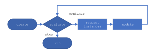
Figure 1: FASL API diagram.

2.3 System Design and User Interface

We implement the AL platform as a REST API with a web frontend. Figure 1 shows the API flow. The Appendix (S. 7) contains screenshots of the UI.

The user first creates a new model (create) by selecting the dataset and label set and label descriptions to use as well as the model type. They can then upload a collection of labeled examples that are used to train the initial model. If no examples are provided the initial model is a zero-shot model.

Afterwards the user can either request instances (request instances) for labeling or run model inference as discussed below. Labeling requires selecting one of the implemented AL methods. Internally the platform annotates the entire unlabeled dataset with new model predictions. The bottleneck is usually the embedding of the input texts using the underlying embedding model. These embeddings are cached to speed up future iterations. Once the instances have been selected, they are shown in the UI. The user now annotates all or a subset of the instances. Optionally, they can reveal the annotation of the current model to ease the annotation work. However, instance predictions are not shown by default to avoid biasing the annotator.

The user can now upload the instances (update) to the platform which results in retraining the underlying few-shot model. At this point, the user can continue to iterate on the model by requesting more instances. When the user is satisfied with the current model they can call model inference on a set of instances (run).

2.4 Performance Prediction

A critical question is how the user knows when to stop annotating (evaluate). To ease their decision making, we add a number of metrics that can be computed even when no test instances is available, which is typically the case in FSL. In particular, we implemented cross-validation on the labeled instances and various metrics that do not require any labels. We collect a random sample $T$ of 1,000 unlabeled training instances. After every AL iteration $i$ we assign the current model distribution $\mathrm{P}_{i}(Y\mid X)$ to these instances. We then define metrics that are computed for every instance and averaged over the entire sample:

• Negative Entropy:
  $-\mathrm{H}_{i}(Y)=\sum_{j}\mathrm{P}_{i}(y_{j}\mid x)\log\mathrm{P}_{i}(y_{j}\mid x)$

• Max Prob: $\mathrm{P}_{i}(\hat{y}\mid x)$, with $\hat{y}_{i}$ as the most probable class

• Margin: $\left[\mathrm{P}_{i}(\hat{y}_{i,1}\mid x)-\mathrm{P}_{i}(\hat{y}_{i,2}\mid x)\right]$, with $\hat{y}_{i,k}$ as kth most probable class

• Negative Update Rate: $\delta(\hat{y}_{i-1}(x),\hat{y}_{i}(x))$, with $\delta$ as the Kronecker delta

• Negative Kullback-Leibler divergence: $-\displaystyle D_{\text{KL}}(P_{i}\parallel P_{i-1})$

Entropy, max prob and margin are based on the uncertainty measure used in AL. The intuition is that the uncertainty of the model is reduced and converges as the model is trained. The update rate denotes the relative number of instances with a different model prediction as in the previous iteration. Again we assume that this rate lowers and converges as the model training converges. The KL divergence provides a more sensitive version of the update rate that considers the entire label distribution.

We also experiment with combining these signals in a random forest regressor (RFR) Ho (1995). For every iteration $i$ the model predicts the normalized test F1. In general, it is hard to predict the true F1 for an unknown classification problem and dataset without even knowing the test set. Therefore, we normalize all target test F1 curves by dividing by their maximum value (Figure 3). Intuitively, the RFR tells us how much of the performance that we will ever reach on this task we have reached so far.

The feature set of the model consists of a few base features such as the number of instances the model has been trained with, the AL method used and the number of labels. Additionally, for each of the metrics above, we add the value at the current iteration $i$ as well as of a history of the last $h=5$ iterations.

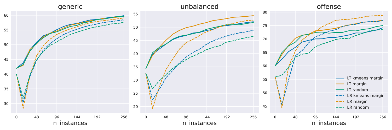
Figure 2: Average test macro F1 score on the generic, unbalanced and offensive datasets. LT and LR denote label tuning and logistic regression, respectively.

Generic	name	gnad	azn-de	ag-news	azn-en	azn-es	hqa	mean
	LT random	72.31.4	47.70.6	85.31.0	48.31.1	46.41.5	57.71.6	59.6
	LT kmeans margin	74.61.1	47.51.6	86.00.4	46.71.4	45.91.7	58.50.9	59.9
	LT kmedoids margin	73.81.5	45.91.9	86.00.5	48.31.3	46.31.3	57.81.4	59.7
	LT margin	74.91.5	45.51.3	86.20.7	46.61.4	46.01.4	58.60.9	59.7
	LT kmedoids	70.92.5	47.51.2	84.91.0	48.11.1	46.71.6	56.91.1	59.1
	LT k-means	70.91.2	47.41.7	82.81.2	48.60.9	46.01.3	55.41.2	58.5
	LT CAL	69.52.3	47.01.4	84.40.7	47.91.6	46.01.1	56.02.4	58.5
	LT kmedoids entropy	73.31.2	41.12.6	85.10.6	43.22.6	41.62.1	57.71.5	57.0
	LT kmedoids least	72.41.3	42.62.0	85.20.5	43.91.8	40.32.6	57.51.3	57.0
	LT entropy	72.12.1	40.22.3	84.70.7	41.32.5	39.92.2	56.51.9	55.8
Unbalanced	LT random	62.66.6	38.82.4	81.91.0	39.22.5	42.53.0	45.52.0	51.8
	LT margin	70.72.2	40.52.4	83.70.8	41.62.9	41.82.4	47.91.5	54.4
	LT CAL	65.23.4	41.12.9	82.01.1	43.81.5	42.92.2	48.41.8	53.9
	LT entropy	70.81.7	40.51.9	82.51.3	38.53.1	39.71.4	47.62.7	53.2
	LT kmedoids least	65.42.8	39.22.1	83.20.9	42.52.1	39.23.0	48.01.5	52.9
	LT least confidence	69.12.4	38.42.1	83.50.7	39.72.0	38.81.5	46.42.4	52.7
	LT kmedoids margin	62.05.0	40.53.0	83.60.5	40.81.6	40.62.4	47.41.9	52.5
	LT kmedoids entropy	64.12.9	39.02.6	82.61.0	39.61.8	40.41.1	47.62.4	52.2
	LT kmeans margin	66.85.1	37.42.8	82.41.3	39.92.0	38.81.7	47.01.5	52.1
	LT kmedoids	59.56.8	37.63.3	81.01.6	41.31.7	41.62.4	44.81.6	51.0
Offense	name	hate	solid					mean
	LR random	61.84.6	85.21.9					73.5
	LR margin	69.11.8	88.30.6					78.7
	LR least confidence	68.92.2	87.80.5					78.3
	LR entropy	68.82.2	87.80.6					78.3
	LR CAL	68.32.6	87.20.9					77.7
	LR kmedoids least	66.72.1	87.50.9					77.1
	LR kmedoids margin	66.42.4	87.31.0					76.9
	LR kmeans margin	66.31.9	87.40.9					76.8
	LR kmedoids entropy	66.12.2	87.60.7					76.8
	LR kmedoids	64.83.7	86.80.9					75.8

Table 1: Average test macro F1 score on the generic, unbalanced and offense datasets for 256 instances. LT and LR denote label tuning and logistic regression. The subscript denotes the standard deviation and bold font indicates the column-wise maximum.

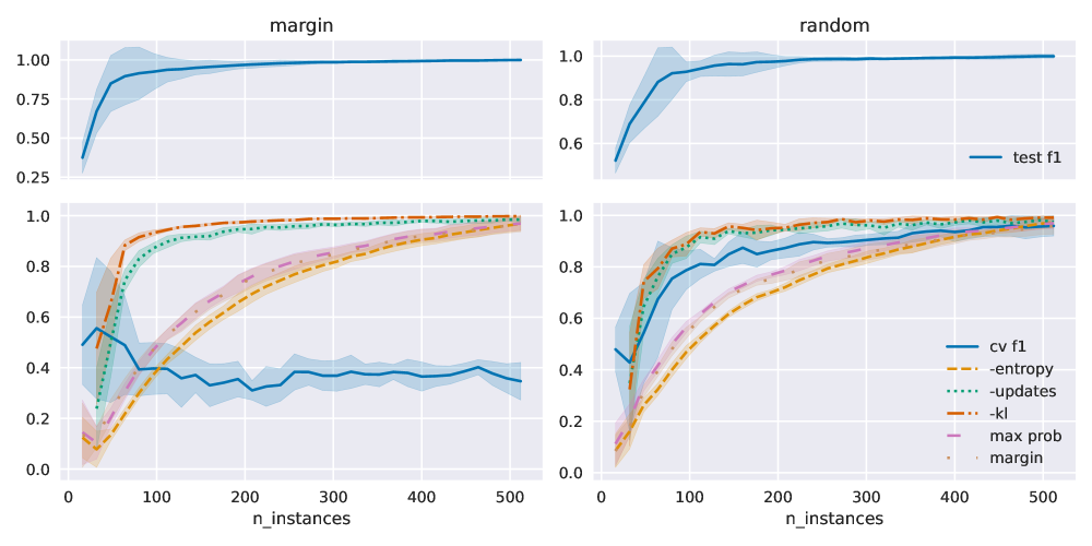
Figure 3: Training metrics for AG-news for the random and margin AL methods. The upper plot shows the true average normalized test F1 (blue curve) as well as the average error of the regressor model (blue shade). The lower plot shows the raw training metrics.

model	MSE	AUC	$\mathcal{F}_{1}$	$\mathcal{P}$	$\mathcal{R}$	test F1	err	instances
baseline 272	3483.2	86.6	80.4	81.2	86.8	94.3	2.0	272.0
baseline 288	3759.8	86.3	80.0	83.1	84.0	94.6	1.8	288.0
baseline 304	4038.8	85.9	79.4	85.1	81.1	95.2	1.4	304.0
base	73.5	97.3	76.5	83.1	80.1	93.9	2.5	284.6
forward cv-f1	56.5	96.9	80.7	84.0	83.8	94.5	1.8	271.8
forward -entropy	70.8	96.4	79.1	84.5	80.9	94.3	2.1	283.5
forward -updates	61.1	96.6	80.2	86.0	81.1	94.7	1.5	284.4
forward -kl	77.1	96.6	75.0	84.3	76.0	94.3	2.3	295.1
forward max-prob	59.9	96.9	80.4	86.0	80.4	95.0	1.4	288.1
forward margin	59.4	96.9	79.2	86.7	78.3	95.0	1.4	294.2
all	65.9	97.1	80.4	86.2	81.6	95.1	1.3	287.3
all h=0	56.0	97.1	79.7	84.7	81.3	94.3	2.0	277.1
all h=1	57.4	97.1	80.7	85.4	82.4	94.5	1.7	276.6
backward cv-f1	66.7	96.7	80.6	84.7	82.8	94.7	1.7	280.2
backward -entropy	57.0	97.0	80.7	86.1	81.9	95.0	1.3	285.5
backward -updates	64.5	97.1	80.4	86.3	81.1	95.0	1.4	288.6
backward -kl	68.0	97.2	81.2	86.7	82.4	95.2	1.2	287.9
backward max-prob	65.7	97.1	80.3	86.5	81.2	95.0	1.3	288.6
backward margin	63.8	97.1	80.2	86.1	81.0	95.0	1.4	289.8

Table 2: Results on the prediction of the test F1: Mean squared error (MSE in ‱), Area under curve (AUC), precision ($\mathcal{P}$), recall ($\mathcal{R}$) and $\mathcal{F}_{1}$ as well as average test F1, error and number of training instances reached at a threshold of $\tau=0.95$. baseline i indicates a baseline that predict 0 for every step $j:j<i$ and 1 otherwise. base is the base feature set discussed in S. 2.4. all uses all features. forward and backward denote ablation experiments with forward selection from base and backward selection from all, respectively. $h$ indicates the size of the history and is 5 by default.

3 Related Work

Active Learning Methods

We evaluate AL methods that have been reported to give strong results in the literature. Within uncertainty sampling, margin sampling has been found to out-perform other methods also for modern model architectures Schröder et al. (2021); Lu and MacNamee (2020). Regarding methods that combine uncertainty and diversity sampling, CAL Margatina et al. (2021) has been reported to give consistently better results than BADGE Ash et al. (2020) and ALPS Yuan et al. (2020) on a range of datasets. A line of research that we exclude are Bayesian approaches such as BALD Houlsby et al. (2011), because the requirement of a model ensemble makes them computationally inefficient.

Few-Shot Learning with Label Tuning

Our work differs from much of the related work in that we use a particular model and training regimen: label tuning (LT) Müller et al. (2022). LT is an approach that only tunes a relative small set of parameters, while the underlying Siamese Network model Reimers and Gurevych (2019) remains unchanged. This makes training fast and deployment scalable. More details are given in Section 2.2.

Cold Start

Cold start refers to the zero-shot case where we start without any training examples. Most studies Ash et al. (2020); Margatina et al. (2021) do not work in this setup and start with a seed set of 100 to several thousand labeled examples. Grießhaber et al. (2020); Schröder et al. (2021); Lu and MacNamee (2020) use few-shot ranges of less than thousand training examples but still use a seed set. Yuan et al. (2020) approach a zero-shot setting without an initial seed set but they differs from our work in model architecture and training regimen.

Balanced and Unbalanced Datasets

Some studies have pointed out inconsistencies on how AL algorithms behave across different models or datasets Lowell et al. (2019). It is further known in the scientific community that AL often does not out-perform random selection when the label distribution is balanced. Ein-Dor et al. (2020) focus on unbalanced datasets but not with a cold start scenario. To fill this gap, we run a large study on AL in the under-researched few-shot-with-cold-start scenario, looking into both balanced and unbalanced datasets.

4 Experimental Setup

We compare a number of active learning models on a wide range of datasets.

	dataset	train	test	$|L|$	$U_{\%}$
Generic	gnad Block (2019)	9,245	1,028	9	34.4
	AG-news Gulli (2005)	120,000	7,600	4	0.0
	hqa Vilares and Gómez-Rodríguez (2019)	4,023	2,742	6	2.8
	azn-de Keung et al. (2020)	205,000	5,000	5	0.0
	azn-en	205,000	5,000	5	0.0
	azn-es	205,000	5,000	5	0.0
Unbalanced	gnad	3,307	370	9	92.9
	AG-news	56,250	3,563	4	60.0
	hqa	1,373	927	6	82.9
	azn-de	79,438	1,938	5	74.8
	azn-en	79,438	1,938	5	74.8
	azn-es	79,438	1,938	5	74.8
Offense	hate de Gibert et al. (2018)	8,703	2,000	2	77.8
	solid Rosenthal et al. (2020)	1,887	2,000	2	45.6

Table 3: Dataset statistics. train and test sizes of the splits. $|L|$ is the cardinality of the label set $L$. $\mathrm{U}$ quantifies the uniformness: $\sum_{l\in L}\left|f(l)-\frac{1}{|L|}\right|$, where $f(l)$ is the relative frequency of label $l$. $U=0$ indicates that the data is distributed uniformly. Note that the generic datasets are balanced while the others are skewed.

4.1 Datasets

Generic Datasets

We run experiments on 4 generic text classification datasets in 3 different languages. AG News (AG-news) Gulli (2005) and GNAD (gnad) Block (2019) are news topic classification tasks in English and German, respectively. Head QA (hqa) Vilares and Gómez-Rodríguez (2019) is a Spanish catalogue of questions in a health domain that are grouped into categories such as medicine, biology and pharmacy. Amazon Reviews (azn) Keung et al. (2020) is a large corpus of product reviews with a 5-star rating in multiple languages. Here we use the English, Spanish and German portion.

Unbalanced Datasets

All of these datasets have a relatively even label distribution. To investigate the performance of AL in a more difficult setup, we also create a version of each dataset where we enforce a label distribution with exponential decay. We implement this by down-sampling some of the labels, without replacement. In particular, we use the adjusted frequency $n^{\prime}(y)=n(\hat{y})^{-2\cdot\operatorname{rank}(y)}$, where $n(y)$ is the original frequency of label $y$, $\hat{y}$ is the most frequent label and $\operatorname{rank}(y)$ is the frequency rank with $\operatorname{rank}(\hat{y})=0$.

Offensive Language Datasets

We also evaluate on the Semi-Supervised Offensive Language Identification Dataset (solid) Rosenthal et al. (2020) and HateSpeech 2018 (hate) de Gibert et al. (2018). These dataset are naturally unbalanced and thus suited for AL experiments.

Table 3 provides statistics on the individual datasets. Note that – following other work in few-shot learning Wang et al. (2021); Schick and Schütze (2021) – we do not use a validation set. This is because in a real world FSL setup one would also not have access to any kind of evaluation data. As a consequence, we do not tune hyper-parameters in any way and use the defaults of the respective frameworks. The label descriptions we use are taken from the related work Wang et al. (2021); Müller et al. (2022) and can be found in the Appendix (S. 7).

4.2 Simulated User Experiments

It is common practice Lowell et al. (2019) in AL research to simulate the annotation process using labeled datasets. For every batch of selected instances, the gold labels are revealed, simulating the labeling process of a human annotator. Naturally, a simulation is not equivalent to real user studies and certain aspects of the model cannot be evaluated. For example, some methods might retrieve harder or more ambiguous examples that will result in more costly annotation and a higher error rate. Still we chose simulation in our experiments as they are a scalable and reproducible way to compare the quality of a large number of different methods. In all experiments, we start with a zero-shot model that has not been trained on any instances. This sets this work apart from most related work that starts with a model trained on a large seed set of usually thousands of examples. We then iteratively select batches of $k=16$ instances until we reach a training set size of 256. The instances are selected from the entire training set of the respective dataset. However, to reduce the computational cost we down-sample each training set to at most 20,000 examples.

As FSL with few instances is prone to yield high variance on the test predictions we average all experiments over 10 random trials. We also increase the randomness of the instance selection by first selecting $2k$ instances with the respective method and later sampling $k$ random examples from the initial selection.

5 Results

Active Learning Methods

Figure 2 shows the AL progression averaged over multiple datasets. For improved clarity only the best performing methods are shown. Plots for the individual dataset can be found in the Appendix (S. 7). On the comparison between Label Tuning (LT) and Logistic Regression (LR) we find that LT outperforms LR on the generic datasets as well as the unbalanced datasets. On the offense datasets the results are mixed: LR outperforms LT when using margin, but is outperformed when using random.

With respect to the best performing selection methods we find that random and margin perform equally well on the generic datasets when LT is used. However, when using LR or facing unbalanced label distributions, we see that margin gives better results than random. On the offense datasets we also find substantial differences between margin and random.

Regarding kmeans-margin, we see mixed results. In general, kmeans-margin does not outperform random when LT is used but does so when LR is used. In most experiments kmeans-margin is inferior to margin.

Table 1 shows results by dataset for the 10 best performing methods. For each set of datasets we include the 10 best performing methods of the best performing model type. We find that uncertainty sampling (such as margin and least-confidence) methods outperform diversity sampling methods (such as kmeans and kmedoids). Hybrid methods such as (CAL and kmeans-margin) perform better than pure diversity sampling methods but are in general behind their counterparts based on importance sampling.

Test F1 Prediction Experiments

We test the F1 regression models with the margin and random AL method. We trained the LR model with $k=16$ instances per iteration until reaching a training set size of 512. As for the AL experiments above we repeat every training run 10 times. We then train a prediction model for each of the 12 datasets used in this study (leaving out one dataset at a time).

Figure 3 shows the model trained for AG-news. We see that the cross-validation F1 computed on the labeled instances (cv f1) has a similar trend as the test F1 when we use random selection. However, when using AL with margin selection the curve changes drastically. This indicates that CV is not a good evaluation method or stopping criterion when using AL. The uncertainty based metrics (max prob, margin and -entropy) correlate better with test F1 but still behave differently in terms of convergence. Negative KL divergence (-kl) and update rate (-updates) on the other hand show a stronger correlation. With regard to the regressor model we can see that the average error (shaded blue area) is large in the beginning but drops to a negligible amount as we reach the center of the training curve.

For evaluating the model, we compute a range of metrics (Table 2). Mean squared error (MSE) is a standard regression metric but not suited to the problem as it overemphasizes the errors at the beginning of the curve. Therefore we define $\tau=0.95$ as the threshold that we are most interested in. That is, we assume that the user wants to train the model until reaching 95% of the possible test F1. With $\tau$ we can define a binary classification task and compute AUC, recall ($\mathcal{R}$), precision ($\mathcal{P}$) and $\mathcal{F}_{1}$. Additionally, we compute the average test-F1, error (err) and training set size when the model first predicts a value $>\tau$.

In the ablation study with forward selection, we find that all features except -entropy and -kl lower the error rate (err) compared to base. For backward selection, only removing cv f1 causes a bigger increase in error rate compared to all. This might be because the unsupervised metrics are strongly correlated. Finally, reducing the history (S. 2.4) also causes an increase in error rate.

In comparison with the simple baselines (baseline $i$), where we simply stop after a fixed number of instances $i$, we find that all gives higher test-f1 (95.1 vs 94.6) at comparable instance numbers (287 vs 288). This indicates that a regression model adds value for the user.

6 Conclusion

We studied the problem of active learning in a few-shot setting. We found that margin selection outperforms random selection for most models and setups, unless the labels of the task are distributed uniformly. We also looked into the problem of performance prediction to compensate the missing validation set in FSL. We showed that the normalized F1 on unseen test data can be approximated with a random forest regressor (RFR) using signals computed on unlabeled instances. In particular, we showed that the RFR peforms better than the baseline of stopping after a fixed number of steps. Our findings have been integrated into FASL, a uniform platform with a UI that allows non-experts to create text classification models with little effort and expertise.

7 Appendix

The repository at https://tinyurl.com/fasl-gh contains the label descriptions, UI screenshots and additional plots and results for active learning and performance prediction.

References

- Ash et al. (2020) Jordan T. Ash, Chicheng Zhang, Akshay Krishnamurthy, John Langford, and Alekh Agarwal. 2020. Deep batch active learning by diverse, uncertain gradient lower bounds. ArXiv, abs/1906.03671.
- Block (2019) Timo Block. 2019. Ten thousand german news articles dataset. https://tblock.github.io/10kGNAD/. Accessed: 2021-08-25.
- Boney and Ilin (2017) Rinu Boney and Alexander Ilin. 2017. Semi-supervised few-shot learning with prototypical networks. CoRR, abs/1711.10856.
- Bowman et al. (2015) Samuel R. Bowman, Gabor Angeli, Christopher Potts, and Christopher D. Manning. 2015. A large annotated corpus for learning natural language inference. In Proceedings of the 2015 Conference on Empirical Methods in Natural Language Processing, pages 632–642, Lisbon, Portugal. Association for Computational Linguistics.
- Dasgupta (2011) Sanjoy Dasgupta. 2011. Two faces of active learning. Theoretical Computer Science, 412(19):1767–1781. Algorithmic Learning Theory (ALT 2009).
- de Gibert et al. (2018) Ona de Gibert, Naiara Perez, Aitor García-Pablos, and Montse Cuadros. 2018. Hate Speech Dataset from a White Supremacy Forum. In Proceedings of the 2nd Workshop on Abusive Language Online (ALW2), pages 11–20, Brussels, Belgium. Association for Computational Linguistics.
- Ein-Dor et al. (2020) Liat Ein-Dor, Alon Halfon, Ariel Gera, Eyal Shnarch, Lena Dankin, Leshem Choshen, Marina Danilevsky, Ranit Aharonov, Yoav Katz, and Noam Slonim. 2020. Active Learning for BERT: An Empirical Study. In Proceedings of the 2020 Conference on Empirical Methods in Natural Language Processing (EMNLP), pages 7949–7962, Online. Association for Computational Linguistics.
- Grießhaber et al. (2020) Daniel Grießhaber, Johannes Maucher, and Ngoc Thang Vu. 2020. Fine-tuning BERT for low-resource natural language understanding via active learning. In Proceedings of the 28th International Conference on Computational Linguistics, pages 1158–1171, Barcelona, Spain (Online). International Committee on Computational Linguistics.
- Gulli (2005) Antonio Gulli. 2005. AG’s corpus of news articles. http://groups.di.unipi.it/~gulli/AG_corpus_of_news_articles.html. Accessed: 2021-07-08.
- Halder et al. (2020) Kishaloy Halder, Alan Akbik, Josip Krapac, and Roland Vollgraf. 2020. Task-aware representation of sentences for generic text classification. In Proceedings of the 28th International Conference on Computational Linguistics, pages 3202–3213, Barcelona, Spain (Online). International Committee on Computational Linguistics.
- Ho (1995) Tin Kam Ho. 1995. Random decision forests. In Proceedings of 3rd international conference on document analysis and recognition, volume 1, pages 278–282. IEEE.
- Houlsby et al. (2011) Neil Houlsby, Ferenc Huszár, Zoubin Ghahramani, and Máté Lengyel. 2011. Bayesian active learning for classification and preference learning. ArXiv, abs/1112.5745.
- Keung et al. (2020) Phillip Keung, Yichao Lu, György Szarvas, and Noah A. Smith. 2020. The multilingual amazon reviews corpus. CoRR, abs/2010.02573.
- Lewis and Gale (1994) David D Lewis and William A Gale. 1994. A sequential algorithm for training text classifiers. In SIGIR’94, pages 3–12. Springer.
- Liu et al. (2019) Yinhan Liu, Myle Ott, Naman Goyal, Jingfei Du, Mandar Joshi, Danqi Chen, Omer Levy, Mike Lewis, Luke Zettlemoyer, and Veselin Stoyanov. 2019. Roberta: A robustly optimized BERT pretraining approach. CoRR, abs/1907.11692.
- Lloyd (1982) S. Lloyd. 1982. Least squares quantization in pcm. IEEE Transactions on Information Theory, 28(2):129–137.
- Lowell et al. (2019) David Lowell, Zachary Chase Lipton, and Byron C. Wallace. 2019. Practical obstacles to deploying active learning. In EMNLP.
- Lu and MacNamee (2020) Jinghui Lu and Brian MacNamee. 2020. Investigating the effectiveness of representations based on pretrained transformer-based language models in active learning for labelling text datasets. ArXiv, abs/2004.13138.
- Margatina et al. (2021) Katerina Margatina, Giorgos Vernikos, Loïc Barrault, and Nikolaos Aletras. 2021. Active learning by acquiring contrastive examples. In Proceedings of the 2021 Conference on Empirical Methods in Natural Language Processing, pages 650–663, Online and Punta Cana, Dominican Republic. Association for Computational Linguistics.
- Müller et al. (2022) Thomas Müller, Guillermo Pérez-Torró, and Marc Franco-Salvador. 2022. Few-Shot Learning with Siamese Networks and Label Tuning. In ACL.
- Nguyen and Smeulders (2004) Hieu Tat Nguyen and Arnold W. M. Smeulders. 2004. Active learning using pre-clustering. Proceedings of the twenty-first international conference on Machine learning.
- Park and Jun (2009) Hae-Sang Park and Chi-Hyuck Jun. 2009. A simple and fast algorithm for k-medoids clustering. Expert Syst. Appl., 36:3336–3341.
- Pedregosa et al. (2011) F. Pedregosa, G. Varoquaux, A. Gramfort, V. Michel, B. Thirion, O. Grisel, M. Blondel, P. Prettenhofer, R. Weiss, V. Dubourg, J. Vanderplas, A. Passos, D. Cournapeau, M. Brucher, M. Perrot, and E. Duchesnay. 2011. Scikit-learn: Machine learning in Python. Journal of Machine Learning Research, 12:2825–2830.
- Reimers and Gurevych (2019) Nils Reimers and Iryna Gurevych. 2019. Sentence-bert: Sentence embeddings using siamese bert-networks. In Proceedings of the 2019 Conference on Empirical Methods in Natural Language Processing. Association for Computational Linguistics.
- Rosenthal et al. (2020) Sara Rosenthal, Pepa Atanasova, Georgi Karadzhov, Marcos Zampieri, and Preslav Nakov. 2020. A large-scale semi-supervised dataset for offensive language identification. arXiv preprint arXiv:2004.14454.
- Schick and Schütze (2021) Timo Schick and Hinrich Schütze. 2021. Exploiting cloze-questions for few-shot text classification and natural language inference. In Proceedings of the 16th Conference of the European Chapter of the Association for Computational Linguistics: Main Volume, pages 255–269, Online. Association for Computational Linguistics.
- Schröder et al. (2021) Christopher Schröder, Andreas Niekler, and Martin Potthast. 2021. Uncertainty-based query strategies for active learning with transformers. ArXiv, abs/2107.05687.
- Settles (2009) Burr Settles. 2009. Active learning literature survey. Computer Sciences Technical Report 1648, University of Wisconsin–Madison.
- Vilares and Gómez-Rodríguez (2019) David Vilares and Carlos Gómez-Rodríguez. 2019. HEAD-QA: A healthcare dataset for complex reasoning. In Proceedings of the 57th Annual Meeting of the Association for Computational Linguistics, pages 960–966, Florence, Italy. Association for Computational Linguistics.
- Wang et al. (2021) Sinong Wang, Han Fang, Madian Khabsa, Hanzi Mao, and Hao Ma. 2021. Entailment as few-shot learner. ArXiv, abs/2104.14690.
- Yin et al. (2019) Wenpeng Yin, Jamaal Hay, and Dan Roth. 2019. Benchmarking zero-shot text classification: Datasets, evaluation and entailment approach. In Proceedings of the 2019 Conference on Empirical Methods in Natural Language Processing and the 9th International Joint Conference on Natural Language Processing (EMNLP-IJCNLP), pages 3914–3923, Hong Kong, China. Association for Computational Linguistics.
- Yin et al. (2020) Wenpeng Yin, Nazneen Fatema Rajani, Dragomir Radev, Richard Socher, and Caiming Xiong. 2020. Universal natural language processing with limited annotations: Try few-shot textual entailment as a start. In Proceedings of the 2020 Conference on Empirical Methods in Natural Language Processing (EMNLP), pages 8229–8239, Online. Association for Computational Linguistics.
- Yuan et al. (2020) Michelle Yuan, Hsuan-Tien Lin, and Jordan L. Boyd-Graber. 2020. Cold-start active learning through self-supervised language modeling. In EMNLP.