Online Caching with no Regret: Optimistic Learning via Recommendations

Abstract

The design of effective online caching policies is an increasingly important problem for content distribution networks, online social networks and edge computing services, among other areas. This paper proposes a new algorithmic toolbox for tackling this problem through the lens of optimistic online learning. We build upon the Follow-the-Regularized-Leader (FTRL) framework, which is developed further here to include predictions for the file requests, and we design online caching algorithms for bipartite networks with pre-reserved or dynamic storage subject to time-average budget constraints. The predictions are provided by a content recommendation system that influences the users viewing activity and hence can naturally reduce the caching network’s uncertainty about future requests. We also extend the framework to learn and utilize the best request predictor in cases where many are available. We prove that the proposed optimistic learning caching policies can achieve sub-zero performance loss (regret) for perfect predictions, and maintain the sub-linear regret bound $O(\sqrt{T})$, which is the best achievable bound for policies that do not use predictions, even for arbitrary-bad predictions. The performance of the proposed algorithms is evaluated with detailed trace-driven numerical tests.

1 Introduction

1.1 Motivation and Background

The quest for efficient data caching policies spans more than 50 years and remains today one of the most important research areas for wireless and wired communication systems [2]. Caching was first studied in computer systems where the aim was to decide which files to store in fast-accessible memory segments (paging) [3]. Its scope was later expanded due to the explosion of Internet web traffic [4] and the advent of content distribution networks (CDNs) [5], and was recently revisited as a technique to improve the operation of wireless networks through edge caches [6] and on-device caching [7]. A common challenge in these systems is to design an online policy that decides which files to store at a cache, without knowing the future file requests, so as to maximize the cache hits or some other cache-related performance metric.

There is a range of online caching policies that tackle this problem under different assumptions on the request arrivals. Policies such as the LFU and LRU are widely-deployed, yet their performance deteriorates when the file popularity is non-stationary, i.e., the requests are drawn from a time-varying probability distribution [8, 9, 10]. This motivated modeling non-stationary request patterns [11, 12] and optimizing accordingly the caching decisions [13, 14]. Another line of work relies on techniques such as reinforcement learning to estimate the request probabilities and make caching decisions accordingly [15, 16]; but typically these solutions either do not offer optimality bounds, or do not scale due to having the library size in their bounds.

Caching was studied within the framework of online learning in [17] for a single-cache system; and in its more general form recently in [18] that proposed an online gradient descent (OGD) caching policy. Interesting follow-up works include sub-modular policies [19], online mirror-descent policies [20], and the characterization of their performance limits [21, 22]. The advantage of these online learning-based caching policies is that they are scalable, do not require training data, and their performance bounds are robust to any possible request pattern, even when the requests are generated by an adversary that aims to degrade the caching operation.

Nevertheless, an aspect that remains hitherto unexplored is whether predictions about future requests can improve the performance of such learning-based caching policies without sacrificing their robustness. This is important in modern caching systems where often the users receive content viewing recommendations from a recommendation system (rec-sys). For instance, recommendations are a standard feature in streaming platforms such as YouTube and Netflix [23]; but also in online social network platforms such as Facebook and Twitter, which moderate the users’ viewing feeds [24]. Not surprisingly, the interplay between recommendations and caching attracted recent attention and prior works aimed to increase the caching hits or reduce routing costs, by either recommending already-cached files to users, or through the joint optimization of caching and recommendation decisions [25, 26, 27, 28, 29]. These important works, however, consider static caching models and require knowing in advance the users’ expected requests and their propensity to follow the recommendations.

Changing vantage point, one can observe that since recommendations bias the users towards viewing certain contents, they can effectively serve as predictions of the forthcoming requests. This prediction information, if properly employed, can hugely improve the efficacy of dynamic caching policies, transforming their design from an online learning to an online optimization problem. Nevertheless, the caching policy needs to adapt to the accuracy of recommendations (i.e., of the predictions) and the users propensity to follow them – which is typically unknown and potentially time-varying. Otherwise, the caching performance might as well deteriorate by following these misleading hints about the future requests. The goal of this work is to tackle exactly this challenging new problem and answer the question: Can we leverage untrusted predictions in caching systems?. We answer this question in the affirmative by proposing online learning-based caching policies that utilize predictions (of unknown quality) to boost performance, if those predictions are accurate, while still maintaining robust performance bounds otherwise.

1.2 Methodology and Contributions

Our approach is based on the theory of Online Convex Optimization (OCO) that was introduced in [30] and has since been applied in several decision problems [31]. The basic premise of OCO is that a learner (here the caching system) selects in each slot $t$ a decision vector $x_{t}$ from a convex set $\mathcal{X}$, without knowing the $t$-slot convex performance function $f_{t}(x)$, that changes with time. The learner’s goal is to minimize the growth rate of regret $R_{T}\!=\!\sum_{t=1}^{T}f_{t}(x^{\star})\!-\!f_{t}(x_{t})$, where $x^{\star}\!=\!\arg\max_{x\in\mathcal{X}}\sum_{t=1}^{T}f_{t}(x)$ is the benchmark solution designed with hindsight, i.e., with access to the entire sequence of future functions $\{f_{t}\}_{t=1}^{T}$. The online caching problem fits squarely in this setup, where $f_{t}(x)$ depends on the users requests and is unknown when the caching is decided. And previous works [18, 19, 20, 21] have proved that OCO-based caching policies achieve $R_{T}\!=\!O(\sqrt{T})$, thus ensuring asymptotically zero average regret: $\lim_{T\rightarrow\infty}R_{T}/T\!=\!0$.

Different from these important studies, we extend the learning model to include predictions that are available through the content recommendations. Improving the regret of learning policies via predictions is a relatively new area in machine learning research. For instance, [32] focuses on the competitive-ratio metric and developed algorithms that use untrusted predictions while maintaining worst-case performance bounds; while [33] applied similar ideas to the paging problem. However, it was shown in [34] that such competitive-ratio algorithms cannot ensure sublinear regret, which is the performance criterion we employ here, in line with all recent works [18, 19, 20, 21, 22].

For regret-minimization with predictions, [35] used predictions $\widetilde{c}_{t}$ for the function gradient $c_{t}\!=\!\nabla f_{t}(x_{t})$ with guaranteed quality, i.e., $c_{t}^{\top}\widetilde{c}_{t}\!\geq\!a\|c_{t}\|^{2}$, to reduce $R_{T}$ from $O(\sqrt{T})$ to $O(\log T)$; and [36] enhanced this result by allowing some predictions to fail the quality condition. A different line of works uses regularizing functions which enable the learner to adapt to the predictions’ quality [37], [38]. This idea is more promising for the caching problem where the recommendations might be inaccurate, or followed by the users for only arbitrary time windows; thus, we used it as starting point to develop our caching learning frameworks.

In specific, our approach relies on the Follow-The-Regularized-Leader (FTRL) algorithm [39] which we extend with predictions that offer optimism by reducing the uncertainty about the next-slot functions. We study different versions of the caching problem. First, we design a policy (OFTRL) for the bipartite caching model [6], which generalizes the standard single cache case [17, 33]. Theorem 1 proves that $R_{T}$ is proportional to prediction errors ($\|c_{t}\!-\widetilde{c}_{t}\|^{2},\forall t$) diminishing to zero for perfect predictions; while still meeting the best achievable bound $O(\sqrt{T})$ for the regular OCO setup (i.e., without using predictions) [21] even if all predictions fail. We continue with the elastic caching problem, where the system resizes the used caches at each slot based, e.g., on volatile storage leasing costs [40, 41, 42]. The aim is to maximize the caching utility subject to a time-average budget constraint. This places the problem in the realm of constrained-OCO [43, 44, 45, 46]. Using a new saddle point analysis with predictions, we prove Theorem 2 which reveals how $R_{T}^{(e)}$ and the budget violation $V_{T}^{(e)}$ depend on the cache sizes and prediction errors, and how one can prioritize one metric over the other while achieving sublinear growth rates for both.

The above algorithms utilize the rec-sys as the only source to predict the next time-slot cost $\tilde{c}_{t+1}$. In many cases, however, content providers might have access to multiple such sources. For example, a statistical user profiling model, a deep learning-based predictive model for content request in the next time slot [47], or even another rec-sys, see [48] and follow-up works. Those sources can be used to obtain multiple, and possibly contradicting, predictions. Our final contribution is, therefore, a meta-learning caching framework that utilizes predictions from multiple sources to achieve the same performance as a caching system that used the best such source to start with. We show that the regret in the case of multiple sources can be strictly negative depending on the request sequence and the existence of a high-accuracy predictor. At the same time, the meta-learning caching framework maintains sublinear regret when all predictors fail. Finally, we show that this framework can also be applied in cases with single rec-sys, and discuss its pros and cons compared to the proposed regularization-based optimistic caching solutions.

In summary, the contributions of this work can be grouped as follows:

$\bullet$ Introduces an online learning framework for bipartite and elastic caching networks that leverages predictions to achieve a regret that is upper-bounded by zero for perfect recommendations and sub-linear $O(\sqrt{T})$ for arbitrary bad recommendations. The results are based on a new analysis technique that improves the bounds by a factor of $\sqrt{2}$ compared to the state-of-art optimistic-regret bounds [38], which we used in our recent work [1].

$\bullet$ Introduces a meta-learning framework that can utilize predictions from multiple sources and jointly learns which of them to use, if any at all, and the optimal caching decisions. This framework achieves negative regret in the best case, and sublinear regret in the worst case.

$\bullet$ Evaluates the policies using various request models and real datasets [49, 50] and compares them with (i) the best in hindsight benchmark; and (ii) the online gradient descent policy, which is known to be regret-optimal and outperforms other caching policies [18, 21].

The work presents conceptual innovations, i.e., using recommendations as an untrusted prediction source for caching, and using different online caching algorithms in an optimistic meta-learning algorithm; as well as technical contributions such as the tightened bound of optimistic proximal FTRL (Theorem 1) and the new optimistic proximal FTRL algorithm with budget constraints (Theorem 2). While we focus on data caching, the proposed algorithms can be directly applied to caching of services and code libraries in edge computing systems.

Paper Organization. The rest of this work is organized as follows. Sec. 2 introduces the system model and states formally the problem. Sec. 3 presents the optimistic online caching policy for the bipartite graph, and Sec. 4 presents the respective policy and results for the case of elastic caching systems. Sec. 5 introduces the meta-learning framework with the inclusion of multiple predictors, and Sec. 6 presents our numerical evaluation of the proposed algorithms using synthetic and real traces. We conclude in Sec. 7.

2 System model and Problem Statement

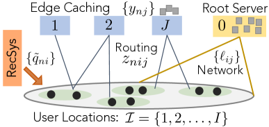
Figure 1: System Model. A network of $\mathcal{J}$ caches serves file requests from a set $\mathcal{I}$ of user locations. Unserved requests are routed to the Root Server. Caching decisions are aided via the recommendations provided by the rec-sys.

2.1 Model Preliminaries

Notation. We use calligraphic capital letters, e.g., $\mathcal{X}$, to denote sets. Vectors are denoted with regular small letters, e.g., $a$, and we use the subscript $t$ to highlight a vector’s dependence on a specific time slot e.g., $a_{t}$. When a compenent of the vector is indexed, the subscript is repurposed to denote that component’s (multi-)index, while the $t$ moves to the superscript. i.e., for the $d$-dimensional vector $a_{t}$ we write $a_{t}=(a^{t}_{1},a^{t}_{2},\ldots,a^{t}_{d})$. We denote with $\{a_{t}\}_{t=1}^{T}$ the sequence of vectors or parameters from slot $t=1$ up to slot $T$; whenever the horizon is not relevant we use $\{a_{t}\}_{t}$. We also use the shorthand sum notation $b_{1:t}=\sum_{i=1}^{T}b_{i}$. We also denote with $[T]$ the integer set ${1,2,\cdots,T}$. The notation for the model and the subsequently presented algorithms is summarized in Table I.

TABLE I: Key Notation

Parameters	Physical Meaning
Caching Network
$\mathcal{J}(J)$	Set (number) of caches
$\mathcal{I}(I)$	Set (number) of user locations
$C_{j}$	Capacity of cache $j$. $C_{j}\leq C,\forall j\!\in\!\mathcal{J}$
$\ell_{ij}$	Indicator for connectivity of location $i$ to cache $j$
$N$	Number of files
$q_{ni}^{t}$	Request issued by user $i$ for file $n$ at slot $t$
$w_{nij}$	Utility for routing a unit of file $n$ from cache $j$ to $i$
$P$	Number of predictors
$c_{t}$	Gradient of the utility function
$\tilde{c}_{t}$	A prediction for $c_{t}$
$s_{j}^{t}$	Price for unit storage in cache $j$
Decision Variables
$y_{nj}^{t}$	Portion of file $n$ stored at cache $j$ at slot $t$
$z_{nij}^{t}$	Portion of file $n$ routed from cache $j$ to $i$ at slot $t$
$x$	A shorthand for the concatenated variables $(y,z)$
Learning Algorithms
$r_{t}(\cdot)$	A strongly convex regularizer function (for $t\geq 1$)
$h_{t}$	Prediction error $\|\tilde{c}_{t}-c_{t}\|$
$\sigma_{t}$	The change in the aggregated root of prediction error $\sqrt{h_{1:t}}-\sqrt{h_{1:t-1}}$
$F_{t}$	Experts performance vector at slot t
$u_{t}$	Weight vector used to combine experts proposals

Network. The caching network includes a set of edge caches ${\cal J}\!=\!\{1,2,\dots,J\}$ and a root cache indexed with 0, as shown in Fig. 1. The file requests emanate from a set of user locations ${\cal I}=\{1,2,\dots,I\}$. The connectivity between $\mathcal{I}$ and $\mathcal{J}$ is modeled with parameters $\ell\!=\!\big{(}\ell_{ij}\in\{0,1\}:i\!\in\!\mathcal{I},j\!\in\!\mathcal{J}\big{)}$, where $\ell_{ij}\!=\!1$ if cache $j$ can be reached from location $i$. We consider the general case where the caches have overlapping coverage; thus, each user can be (potentially) served by one or more edge caching. The root cache is within the range of all users in $\mathcal{I}$. This is a general non-capacitated bipartite model, see [51] for an overview of caching models; and extends the celebrated femtocaching model [6] since the link qualities (which are captured through the utility gains; see below) not only may vary with time, but can do so in an arbitrary (i.e., non-stationary) fashion. This latter feature is particularly important for the realistic modeling of volatile wireless edge caching systems [52, 53].

Requests. The system operation is time slotted, $t\!\!=\!\!1,2,\dots,\!T$. Users submit requests for obtaining files from a library $\mathcal{N}$ of $N$ files with unit size; we note that the analysis can be readily extended to files with different sizes, This will be made clear in Sec. 2.2. Parameter $q^{t}_{ni}\!\in\!\{0,1\}$ indicates the submission of a request for file $n\!\in\!\mathcal{N}$ by a user at location $i\!\in\!\mathcal{I}$ in the beginning of slot $t$. At each slot we assume there is one request; i.e., the caching decisions are updated after every request, as in LFU and LRU policies, [54, 55]. Hence, the request process comprises successive vectors $q_{t}\!=\!(q_{ni}^{t}\!\in\!\{0,1\}:n\!\in\!\mathcal{N},i\!\in\!\mathcal{I})$ from the set:

$$\mathcal{Q}=\bigg{\{}q\in\{0,1\}^{N\cdot I}~{}\Big{|}~{}\sum_{n\in\mathcal{N}}\sum_{i\in\mathcal{I}}q_{ni}=1\bigg{\}}.$$

We make no assumptions for the request pattern; it might follow a fixed or time-varying distribution that is unknown to the system; and can be even selected strategically by an adversary aiming to degrade the caching operation. If a policy’s performance is satisfactory under this model, it is ensured to achieve (at least) the same performance for other request models.

Recommendations. There is a recommender system (rec-sys) that suggests files to each user $i\!\in\!\mathcal{I}$, see [23] for the case of Netflix. User $i$ requests one of the recommended files with a certain probability that captures the user’s propensity to follow the recommendations. Unlike prior works that consider these probabilities fixed (or assume that the recommendation following event is a stationary stochastic process) [56, 25], we model them as unknown and possibly time-varying. Namely, no assumption on their quality is guaranteed to remain valid.

A key point in our approach is that the content recommendations, if properly leveraged, can serve as predictions for the next-slot requests which are otherwise unknown. We denote with $\tilde{q}_{t}$ the prediction for the request $q_{t}$ that the system will receive at the beginning of slot $t$, and we assume that $\tilde{q}_{t}$ is available at the end of slot $t\!-\!1$, i.e., when the rec-sys provides its recommendations. Essentially, the recommender system is an approach for obtaining prediction for the next request. The recommendation can be mapped to predictions in different ways. For example, the caching system can set $\widetilde{q}_{\hat{n}\hat{i}}^{\ t+1}=1$ and $\widetilde{q}_{ni}^{\ t+1}=0,\forall(n,i)\neq(\hat{n},\hat{i})$, where $(\hat{n},\hat{i})$ is the request with the highest predicted probability (top recommended file). In section 5, we study the case where a set $\mathcal{P}=\{1,\ldots,P\}$ of $P$ different predictors (other than the recommendatino system) are available, each one offering a prediction $q_{t}^{(p)},p\in\mathcal{P}$ at every slot $t$.

Caching. Each cache $j\!\in\!\mathcal{J}$ stores up to $C_{j}\!<<\!N$ files, while the root cache stores the entire library, i.e., $C_{0}\!\geq\!N$. We also define $C\!=\!\max_{j\in\mathcal{J}}C_{j}$. Following the standard femtocaching model [6], we perform caching using the Maximum Distance Separable (MDS) codes, where files are split into a fixed number of $F$ chunks, which include redundancy chunks. A user can decode the file if it receives any $F$-sized subset of its chunks. For large values of $F$, the MDS model allows us to use continuous caching variables. Hence, we define the variable $y_{nj}^{t}\!\in\![0,1]$ which denotes the portion of $F$ chunks of file $n\!\in\!\cal N$ stored at cache $j\!\in\!\cal J$, and we introduce the $t$-slot caching vector $y_{t}\!=\!(y_{nj}^{t}:n\!\in\!\mathcal{N},j\!\in\!\mathcal{J})$ that belongs to set:

$$\mathcal{Y}=\bigg{\{}y\in[0,1]^{N\cdot J}~{}\Big{|}~{}\sum_{n\in\mathcal{N}}y_{nj}\leq C_{j},~{}j\in\mathcal{J}\bigg{\}}.$$

Routing. Since each user location $i\in\mathcal{I}$ may be connected to multiple caches, we need to introduce routing variables. Let $z_{nij}^{t}$ denote the portion of request $q_{ni}^{t}$ served by cache $j$. In the MDS caching model the requests can be simultaneously routed from multiple caches and, naturally, we restrict the amount of chunks not to exceed $F$. Hence, the $t$-slot routing vector $z_{t}=(z_{nij}^{t}\!\in\![0,1]:n\!\in\!\mathcal{N},i\!\in\!\mathcal{I},j\!\in\!\mathcal{J})$ is drawn from:

$$\mathcal{Z}=\bigg{\{}z\in[0,1]^{N\cdot J\cdot I}~{}\Big{|}~{}\sum_{j\in\mathcal{J}}z_{nij}\leq 1,~{}n\in\mathcal{N},i\in\mathcal{I}\bigg{\}}.$$

Requests that are not (fully) served by the edge caches $\mathcal{J}$ are served by the root server that provides the missing chunks. This decision needs not to be explicitly modeled as it is directly determined by the routing vector $z_{t}$.

2.2 Problem Statement

Cache Utility & Predictions. We use parameters $w_{nij}\in[0,w]$ to model the system utility when delivering a chunk of file $n\!\in\!\cal N$ to location $i\!\in\!\cal I$ from cache $j\!\in\!\cal J$, instead of using the root server. This utility model can be used to capture bandwidth or delay savings, and other edge-caching gains in wired or wireless networks. The caching benefits can in general differ for each cache and user location, and may vary with time. Note that the cache-hit maximization problem is a special case of this setting [2]. To streamline presentation we introduce vector $x_{t}\!=\!(y_{t},z_{t})\in\mathbb{R}^{m}$, with $m\!=\!NIJ\!+\!NJ$, and define the system utility in slot $t$ as:

$$f_{t}(x_{t})=\sum_{n\in\mathcal{N}}\sum_{i\in\mathcal{I}}\sum_{j\in\mathcal{J}}w_{nij}q^{t}_{ni}z_{nij}^{t}\ ,$$ (1)

and we denote its gradient $c_{t}\!=\!\nabla f_{t}(x_{t})$. As it will become clear, our analysis holds also for non-linear concave functions $f_{t}(x)$; this generalization is useful in case, e.g., we wish to enforce fairness in the dispersion of caching gains across the user locations [41].

The main challenge in online caching is the following: at the end of each slot $t$ where we need to decide the cache configuration, the utility function $f_{t+1}$ is not available. Indeed, this function depends on the next-slot request $q_{t+1}$, which, by the time it gets revealed, $y_{t+1}$ would have already been decided and fixed, see [18, 21, 33]. This is also the timing of the LRU/LFU policies [54, 55]. However, the recommendations provided to users can be used to form a predicted request $\widetilde{q}_{t+1}$. Then, we can use $\widetilde{q}_{t+1}$ to create a prediction for the next slot function $\widetilde{f}_{t+1}(\cdot)$ through its gradient $\widetilde{c}_{t+1}$, (recall that $f_{t+1}(\cdot)$ is a linear function that is parameterized by its gradient $c_{t+1}$).

Benchmark. In such learning problems, it is important to understand the objective that our algorithm aims to achieve. If we had access to an oracle for the requests $\{q_{t}\}_{t=1}^{T}$ (and the utility parameters) we could have devised the utility-maximizing static caching and routing policy $x^{\star}=(y^{\star},z^{\star})$, by solving the following convex optimization problem:

$$\mathbb{P}_{1}:\quad\max_{x}\,\,\,\,\,\, \sum_{t=1}^{T}f_{t}(x)$$ (2)

s.t. $$\,\,z_{nij}\leq y_{nj}\ell_{ij},\quad i\in\mathcal{I},j\in\mathcal{J},n\in\mathcal{N},$$ (3)

$$\,\,z\in\mathcal{Z},\,\,\,\,y\in\mathcal{Y},$$ (4)

where (3) ensure the routing decisions for each requested file use only caches that store enough chunks of that file.Note that the case of files of different sizes corresponds to replacing the set $\mathcal{Y}$ with $\mathcal{Y}^{\prime}=\{y\in[0,1]^{N\cdot J}~{}|~{}\sum_{n\in\mathcal{N}}v_{n}y_{nj}\leq C_{j},~{}j\in\mathcal{J}\}$ For some general size vector $v\in\mathbb{R}_{+}^{N}$. Such a change will not affect the mathematical characteristics of the above optimization problem (both sets correspond to linear constraints).

Let us define the convex set of constraints:

$$\mathcal{X}=\big{\{}\left\{\mathcal{Y}\times\mathcal{Z}\right\}\cap\{\eqref{eq:opt1b}\}\big{\}}$$ (5)

that we will use henceforth to streamline presentation.

Clearly, this hypothetical solution $x^{\star}$ can be designed only with hindsight and is the benchmark for evaluating our online learning policy $\pi$ which outputs $\{x_{t}\}_{t}$. Thus, we use the regret metric:

$$R_{T}(\pi)=\sup_{\{f_{t}\}_{t=1}^{T}}\left[\sum_{t=1}^{T}f_{t}\big{(}x^{\star}\big{)}-\sum_{t=1}^{T}f_{t}\big{(}x_{t}\big{)}\right],$$ (6)

which quantifies the performance gap of $\pi$ from $x^{\star}$, for any possible sequence of requests or, equivalently, functions $\{f_{t}\}_{t}$. Our goal is to find a policy that achieves sublinear regret, $R_{T}(\pi)\!=\!o(T)$, thus ensuring the average performance gap $R_{T}/T$ will diminish as $T$ grows. This policy, similar to other online policies, decides $x_{t+1}$ at the end of each slot $t$ using the previous utility functions $\{f_{\tau}\}_{\tau=1}^{t}$ and the next-slot prediction $\tilde{f}_{t+1}$ devised from the rec-sys.

Lastly, note that, in principle, the regret metric can be negative. This is especially true for optimistic policies. To see why, recall that $x^{\star}$ is the best fixed caching configuration, whereas $x_{t}$ is allowed to change for each $t$. Hence, it might happen, e.g., that $x_{t}$ performs better than $x^{\star}$ on some steps, $f_{t}(x_{t})\geq f_{t}(x^{\star})$, while performing similar to $x^{\star}$ in the remaining ones $f_{t}(x_{t})\approx f_{t}(x^{\star})$. Of course, the occurrence of such an event depends on the request sequence and the policy that determines $x_{t}$. In the following sections, we show that optimism can greatly decrease the upper bound on $R_{T}$, increasing the chances of negative regret.

3 Optimistic Bipartite Caching

Unlike recent caching solutions that rely on Online Gradient Descent (OGD) [18] or on the Follow-the-Perturbed-Leader (FTPL) policy [21], our approach draws from the Follow-The-Regularized-Leader (FTRL) policy, cf. [58], appended with prediction-adaptive regularizers. A key element in our proposal is the optimism emanating from the availability of predictions, namely the content recommendations that are offered to users by the rec-sys in each slot.

Let us begin by defining the proximal regularizers:

$$r_{0}(x)=\bm{I}_{\mathcal{X}}(x),\quad r_{t}(x)=\frac{\sigma_{t}}{2}\|x-x_{t}\|^{2},\,\,t\geq 1$$ (7)

where $\|\cdot\|$ is the Euclidean norm, and $\bm{I}_{\mathcal{X}}(x)\!=\!0$ if $x\!\in\!\mathcal{X}$ and $\infty$ otherwise. We apply properly selected regularizing parameters, which change the strong convexity of $r_{t}$ according to the predictions quality until $t$, and also ensure $r_{t}(x)\geq 0,\forall t$, namely:

$$\sigma_{1}=\sigma\sqrt{h_{1}},\quad\sigma_{t}=\sigma\left(\sqrt{h_{1:t}}-\sqrt{h_{1:t-1}}\right),\quad t\geq 2$$ (8)

$$\text{with}\quad h_{t}=\|c_{t}-\widetilde{c}_{t}\|^{2},$$

where $\sigma\!\geq\!0$, $c_{t}\!=\!\nabla f_{t}(x_{t})$, and we used the shorthand sum notation $h_{1:t}\!=\!\sum_{i=1}^{t}h_{i}$ for the aggregate prediction errors during the first $t$ slots. The basic step of the algorithm is:

$$x_{t+1}=\arg\min_{x\in\mathbb{R}^{m}}\Big{\{}r_{0:t}(x)-(c_{1:t}+\widetilde{c}_{t+1})^{\top}x\Big{\}},$$ (9)

which calculates the decision vector using past utility observations $c_{1:t}$, the aggregate regularizer $r_{0:t}(x)$ and the prediction $\widetilde{c}_{t+1}$. The update employs the negative gradients as it concerns a maximization problem. Henceforth, we refer to (9) as the optimistic FTRL (OFTRL) update.

Policy $\pi_{obc}$ is outlined in Algorithm 1. In each iteration, OBC solves a convex optimization problem, (9), involving a projection on the feasible set $\mathcal{X}$ (via $r_{0}(x)$). For the latter, one can rely on fast-projection algorithms specialized for caching, e.g., see [18]; while it is possible to obtain a closed-form solution for the OFTRL update for linear functions. We quantify next the performance of Algorithm 1.

1 Input: $\{\ell_{ij}\}_{(i,j)}$; $\{C_{j}\}_{j}$; $\mathcal{N}$; $x_{1}\!\in\!\mathcal{X}$; $\sigma=\sqrt{2}/D_{\mathcal{X}}$.

2Output: $x_{t}=(y_{t},z_{t})$, $\forall t$.

3for  $t=1,2,\ldots$  do

      4 Route request $q_{t}$ according to configuration $x_{t}$

      5 Observe system utility $f_{t}(x_{t})$

      6 Observe the new prediction $\widetilde{c}_{t+1}$

      7 Update the regularizer $r_{0:t}(x)$ using (7)-(8)

      8 Calculate the new policy $x_{t+1}$ using (9)

      

end for

Algorithm 1 Optimistic Bipartite Caching ($\pi_{obc}$)

Theorem 1.

Algorithm 1 ensures the regret bound: $\displaystyle R_{T}\leq 2\sqrt{1\!+JC}\sqrt{\sum_{t=1}^{T}\|c_{t}-\widetilde{c}_{t}\|^{2}}.$

For the proof, we modify the “strong FTRL lemma” [58, Lemma 5] by adding predictions for next-slot utility function. The following lemma bounds the regret in terms of the difference between two values of a strongly convex function evaluated at $x_{t}$ and at $x_{t+1}$, for each $t$.

Lemma 1.

(Optimistic Strong FTRL Lemma) Let $v_{t}(x)=-c_{t}^{\top}x_{t}+r_{t}(x_{t})$, and $v_{0:t}(x)=-c_{1:t}^{\top}x_{t}+r_{0:t}(x_{t})$. Let $x_{t+1}$ be selected according to (9). Then:

$$R_{T}\leq r_{0:T}(x^{\star})+\sum_{t=1}^{T}v_{0:t}(x_{t})-v_{0:t}(x_{t+1})-r_{t}(x_{t})\\ +\tilde{c}_{T+1}^{\top}(x_{T+1}-x^{\star})$$ (10)

Proof of Lemma 1.

$$\sum_{t=1}^{T}v_{t}(x_{t})-(v_{0:T}(x^{\star})-\tilde{c}_{T+1}^{\top}x^{\star})$$

$$=\sum_{t=1}^{T}\left(v_{0:t}(x_{t})-v_{0:t-1}(x_{t})\right)-(v_{0:T}(x^{\star})-\tilde{c}_{T+1}^{\top}x^{\star})$$

$$\leq\sum_{t=1}^{T}v_{0:t}(x_{t})+\sum_{t=1}^{T}\left(-v_{0:t-1}(x_{t})\right)$$

$$-(v_{0:T}(x_{T+1})-\tilde{c}_{T+1}^{\top}x_{T+1})\quad\quad(\text{by def. of $x_{T+1}$})$$

$$\stackrel{{\scriptstyle\text{(a)}}}{{\leq}}\sum_{t=1}^{T}v_{0:t}(x_{t})-v_{0}(x_{1})+\sum_{t=1}^{T-1}\left(-v_{0:t}(x_{t+1})\right)$$

$$-v_{0:T}(x_{T+1})+\tilde{c}_{T+1}^{\top}x_{T+1}$$

$$\stackrel{{\scriptstyle\text{(b)}}}{{\leq}}\sum_{t=1}^{T}\big{(}v_{0:t}(x_{t})-v_{0:t}(x_{t+1})\big{)}+\tilde{c}_{T+1}^{\top}x_{T+1}$$ (11)

where equality (a) follows by reindexing the second sum (i.e., changing the sum index from $t$ to $t+1$), and inequality (b) by dropping the non-positive term $-v_{0}(x_{1})=-r_{0}(x_{1})$ and appending the term $-v_{0:T}(x_{T+1})$ to the second sum. Thus, we have that:

$$\sum_{t=1}^{T}v_{t}(x_{t})-v_{0:T}(x^{\star})+\tilde{c}_{T+1}^{\top}x^{\star}$$

$$\leq\sum_{t=1}^{T}\big{(}v_{0:t}(x_{t})-v_{0:t}(x_{t+1})\big{)}+\tilde{c}_{T+1}^{\top}x_{T+1}.$$ (12)

Expanding the definition of $v_{t}(x_{t})$ and rearranging give the regret inequality.

$$c_{0:T}^{\top}x^{\star}-\sum_{t=1}^{T}c_{t}^{\top}x_{t}\leq r_{0:T}(x^{\star})+\sum_{t=1}^{T}\big{(}v_{0:t}(x_{t})-v_{0:t}(x_{t+1})\big{)}\\ -r_{t}(x_{t})+\tilde{c}_{T+1}^{\top}(x_{T+1}-x^{\star}).$$ (13)

∎

With the weak assumption that the caching system will be notified upon the serving of the last request, we can set $\tilde{c}_{T+1}=0$ and hence cancel the last term in the above inequality. Otherwise, it will be an additional constant factor in the regret bound. Next, we will make use of the following results to bound each $v_{0:t}(x_{t})-v_{0:t}(x_{t+1})$ term:

Lemma 2.

[58, Lemma 7] let $\phi_{1}\!:\!\mathbb{R}^{n}\to\!\mathbb{R}$ be a convex function such that $x_{1}\!=\!\arg\min_{x}\phi_{1}$. Let $\psi$ be a convex function such that $\phi_{2}(x)\!=\!\phi_{1}(x)\!+\!\psi(x)$ is strongly convex w.r.t norm $\|\cdot\|$. Then, for any $b\in\partial\psi(x_{1})$ and $x^{\prime}$, we have that $\phi_{2}(x_{1})\!-\!\phi_{2}(x^{{}^{\prime}})\!\leq\!\frac{1}{2}\|b\|_{\star}^{2}$.

Now we are ready to prove Theorem 1:

Proof of Theorem 1.

We start by applying Lemma 2 to the result in (10). Namely, we select:

$$\phi_{1}(x)=v_{0:t}(x)+{c_{t}^{\top}}{x_{t}}-{\tilde{c}_{t}^{\top}}{x_{t}},\,\,\text{and}$$

$$\phi_{2}(x)=\phi_{1}(x)-{c_{t}^{\top}}{x_{t}}+{\tilde{c}_{t}^{\top}}{x_{t}}.$$

This way, we have that $x_{t}\!=\!\arg\min{\phi_{1}(x_{t})}$,  $\phi_{2}(x)\!=\!v_{0:t}(x)$,  $\psi(x)\!=\!(-c_{t}+\tilde{c}_{t})^{\top}x$,  and $(-c_{t}+\tilde{c}_{t})\!\in\!\partial\psi(x)$.

Then, dropping the non-positive terms $-r_{t}(\cdot)$ in (10), setting $\tilde{c}_{T+1}=0$, and defining the norm $\|\cdot\|_{(t)}=\sqrt{\sigma_{1:t}}\|x\|$ so that the regularizer $r_{1:t}(x)$ is 1-strongly-convex w.r.t. $\|\cdot\|_{(t)}$ we get:

$$R_{T}\leq r_{1:T}(x^{\star})+\frac{1}{2}\sum_{t=1}^{T}\|c_{t}-\widetilde{c}_{t}\|_{(t),\star}^{2},\,\,\,\,\forall x^{\star}\in\cal X.$$ (14)

Now, we have that $r_{t}\leq\frac{\sigma_{t}}{2}D_{\mathcal{X}}^{2}$, where $D_{\mathcal{X}}$ is the Euclidean diameter $D_{\mathcal{X}}$, i.e., $\forall x,x_{t}\!\in\!\cal X$:

$$\|x-x_{t}\|^{2} =\sum_{n,j}(y_{nj}-y_{nj}^{t})^{2}+\sum_{n,i,j}(z_{nij}-z_{nij}^{t})^{2}$$

$$\stackrel{{\scriptstyle(a)}}{{\leq}}\sum_{n,j}|y_{nj}-y_{nj}^{t}|+\sum_{n,i,j}|z_{nij}-z_{nij}^{t}|$$

$$\stackrel{{\scriptstyle(b)}}{{\leq}}2(JC+1)\triangleq D_{\mathcal{X}}^{2}$$

where $(a)$ holds as $y_{nj},z_{nij}\!\in\![0,1],\forall n,i,j$; $(b)$ holds by the triangle inequality and definitions of $\mathcal{Y}$, $C\!\triangleq\!\max_{j}C_{j}$, and the fact that the routing variables differ at one coordinate only. To see why, recall that we serve one request per time slot and we set the routing variable $z_{t}$ after observing that request $q_{t}$. Hence, we can modify the routing variables and set $z^{\star}_{nij}=z^{t}_{nij}=0\ \forall n\neq n^{\prime},i\neq i^{\prime},j\neq j^{\prime}$, where $q_{n^{\prime}i^{\prime}}=1\wedge\ell_{i^{\prime}j^{\prime}=1}$. Due to the structure of $f_{t}(\cdot)$, the utility of these modified $z^{\star}_{nij}$ and $z^{t}_{nij}$ will not change (compared to their utility before modification). In words, knowing the requested file $n^{\prime}$, and the location from which it is requested $i^{\prime}$, there will be no utility from routing a non-requested file $n\neq n^{\prime}$, or routing from a non-connected cache $j\neq j^{\prime}$. Thus, we can zero these variables and get a smaller value for $D_{\mathcal{X}}$, without affecting the utility values.

Using this diameter bound, and the fact that the dual norm of $\|x\|_{(t)}$ is $\|x\|_{(t),\star}=\|x\|/\sqrt{\sigma_{1:t}}$, inequality (14) can be written as:

$$R_{T} \leq\frac{\sigma_{1:T}}{2}D_{\mathcal{X}}^{2}+\frac{1}{2}\sum_{t=1}^{T}\frac{h_{t}}{\sigma_{1:t}}.$$ (15)

Note that the sum $\sigma_{1:t}$ telescopes and evaluates to $\sigma\sqrt{h_{1:t}}$. Using this observation and substituting it in (15), and combining it with [61, Lem. 3.5] to bound the second term as follows $\sum_{t}^{T}h_{t}/\sqrt{h_{1:t}}\!\leq\!2\sqrt{h_{1:T}}$, we eventually get:

$$R_{T} \leq\frac{\sigma}{2}\sqrt{h_{1:T}}D_{\mathcal{X}}^{2}+\frac{1}{\sigma}\sqrt{h_{1:T}}\stackrel{{\scriptstyle(a)}}{{\leq}}\sqrt{2}D_{\mathcal{X}}\sqrt{h_{1:T}},$$

where $(a)$ is obtained by setting $\sigma=\sqrt{2}/D_{\mathcal{X}}$. Finally, substituting the actual diameter value, namely $D_{\mathcal{X}}\!\!=\!\!\sqrt{2(JC+1)}$, completes the proof. ∎

Discussion. Theorem (1) shows that the regret does not depend on the library size $N$ and is also modulated by the quality of the predictions; accurate predictions tighten the bound, and in the case of perfect predictions, i.e., when users follow the recommendations, we get negative regret $R_{T}\!\leq\!0,\forall T$, which is much stronger than the sub-linear growth rates in other works [18, 62]. In fact, even when predictions fail for constant number of time slots $L\in[T]$, the regret will be constant of the same order $R_{T}\leq O(L)$, which is still a significant improvement over any time-dependent bound.

On the other hand, for worst-case prediction, we can still use the bound $\|c_{t}-\widetilde{c}_{t}\|^{2}\leq 2w^{2}$, and get:

$$R_{T}\leq 2\sqrt{2}w\sqrt{JC+1}\sqrt{T}=O(\sqrt{T})$$

i.e., the regret is at most a constant factor worse than the regret of those policies that do not incorporate predictions. Thus, OBC offers an efficient and safe approach for incorporating predictions in cases where we are uncertain about their accuracy, e.g., either due to the quality of the rec-sys or the behavior of users.

Another key point is that the utility parameters might vary with time as well. Indeed, replacing $w_{t}=(w_{nij}^{t}\!\leq\!w,n\!\!\in\!\!\mathcal{N},i\!\!\in\!\!\mathcal{I},j\!\!\in\!\!\mathcal{J})$ in $f_{t}(x_{t})$ does not affect the analysis nor the bound. This is important when the caching system employs a wireless network where the link capacities vary, or when the caching utility changes; and we note that this utility can be even file-specific. Parameters $w_{t}$ can be also unknown when $x_{t}$ is decided, exactly as it is with $q_{t}$, and they can be predicted using e.g., channel measurements. Essentially the proposed model drops several restricted assumptions of prior works regarding, not only the knowledge of request rates/densities, but also about the system state, link quality, and user utilities. Finally, we observe that in case the algorithm is used to optimize the operation of an edge computing system, these parameters can capture the potentially time-varying utility of each computation, for each service ($n$) and each pair of user - cache.

On a technical note, Lemma 1 presents a novel theoretical result and enables the improvement of the best known proximal OFTRL bound of [38] by a constant factor of $\sqrt{2}$. This also opens the door for leveraging the modular analysis tools developed in [58] in the optimistic OCO framework for different special cases of the utility functions. This technical result is of independent interest.

Lastly, in the case of more than one request per time slot (e.g., $B$ requests), the Euclidean norm would instead be $D^{2}_{\mathcal{X}}=2(JC+B)$. Therefore, the same results hold (in terms of the regret being always sub-linear and commensurate with the prediction accuracy). However, the worst case bounds will of course be scaled by a factor of $\sqrt{B}$ since now we would use $\|c_{t}-\tilde{c}_{t}\|^{2}\leq 2B\ w^{2}$.

4 Optimistic Caching in Elastic Networks

We extend our analysis to elastic caching networks where the caches can be resized dynamically. Such architectures are important for two reasons. Firstly, there is a growing number of small-size content providers that implement their services by leasing storage on demand from infrastructure providers [63]; and secondly, CDNs often resize their caches responding to the time-varying user needs and operating expenditures [64].

1 Input: $\{\ell_{ij}\}_{(i,j)}$, $\{C_{j}\}_{j}$, $\mathcal{N}$, $\lambda_{1}\!=\!0$, $x_{1}\!\in\!\mathcal{X}_{e}$.

2Output: $x_{t}=(y_{t},z_{t})$, $\forall t$.

3for  $t=1,2,\ldots$  do

      4 Route request $q_{t}$ according to configuration $x_{t}$

      5 Observe system utility $f_{t}(x_{t})$ and cost $g_{t}(x_{t})$

      6 Update the budget parameter $\lambda_{t+1}$ using (20)

      7 Update the regularizers $r_{0:t}(x)$ using (7)-(8), and $a_{t}\!=\!at^{-\beta}$

      8 Observe prediction $\widetilde{c}_{t+1}$ and price $s_{t+1}$

      9 Calculate the new policy $x_{t+1}$ using (21)

      

end for

Algorithm 2 Optimistic Elastic Caching ($\pi_{oec}$)

We introduce the $t$-slot price vector $s_{t}\!=\!(s_{j}^{t}\!\leq\!s,j\!\in\!\mathcal{J})$, where $s_{j}^{t}$ is the leasing price per unit of storage at cache $j$ in slot $t$, and $s$ its maximum value. In the general case, these prices may change arbitrarily over time, e.g., because the provider has a dynamic pricing scheme or the electricity cost changes [40, 41]; hence the caching system has access only to $s_{t}$ at each slot $t$. We denote with $B_{T}$ the budget the system intends to spend during a period of $T$ slots for leasing cache capacity. The objective is to maximize the caching gains while satisfying:

$$\sum_{t=1}^{T}g_{t}(x_{t})=\sum_{t=1}^{T}\sum_{j\in\mathcal{J}}\sum_{n\in\mathcal{N}}s_{j}^{t}y_{nj}^{t}-B_{T}\leq 0.$$ (16)

In particular, the new benchmark problem in this case is:

$$\mathbb{P}_{2}:\quad\max_{x\in\mathcal{X}}\sum_{t=1}^{T}f_{t}(x),\,\,\,\,\,\,\text{s.t.}\sum_{t=1}^{T}g_{t}(x)\leq 0,$$ (17)

which differs from $\mathbb{P}_{1}$ due to the leasing constraint.

Indeed, in this case the regret is defined as:

$$R_{T}^{(e)}(\pi)=\sup_{\{f_{t}\}_{t=1}^{T}}\left[\sum_{t=1}^{T}f_{t}\big{(}x^{\star}\big{)}-\sum_{t=1}^{T}f_{t}\big{(}x_{t}\big{)}\right],$$ (18)

where

$$x^{\star}\!\in\!\mathcal{X}_{e}\triangleq\{x\in\mathcal{X}\mid\eqref{eq:opt1b},g_{t}(x)\leq 0,\forall t\},$$

i.e., $x^{\star}$ is a feasible point of $\mathbb{P}_{2}$ with the additional restriction to satisfy $g_{t}(x)\!\leq\!0$ in every slot. In the definition of $\mathcal{X}$, $C$ now denotes the maximum leasable space. Learning problems with time-varying constraints are hard, see impossibility result in [65], and hence require such additional restrictions on the selected benchmarks. We refer the reader to [43] for a related discussion, and to [44, 45] for different benchmarks. Finally, apart from $R_{T}^{(e)}$, we need also to ensure sublinear growth rate for the budget violation:

$$V_{T}^{(e)}=\sum_{t=1}^{T}\left[g_{t}(x_{t})\right]_{+}.$$

To tackle this new problem we follow a saddle point analysis, which is new in the context of OFTRL.

Namely, we first define a Lagrangian-type function by relaxing the budget constraint and introducing the dual variable $\lambda\geq 0$:

$$\mathcal{L}_{t}(x,\lambda)\!=\!\frac{\sigma_{t}}{2}\|x\!-x_{t}\|^{2}\!-f_{t}(x)\!+\lambda g_{t}(x)\!-\frac{\lambda^{2}}{a_{t}}.$$ (19)

The last term is a non-proximal regularizer for the dual variable; and we use $a_{t}\!=\!at^{-\beta}$, where parameter $\beta\!\in\![0,1)$ can be used to prioritize either $R_{T}^{(e)}$ or $V_{T}^{(e)}$. The main ingredients of policy $\pi_{oec}$ are the saddle-point iterations:

$$\lambda_{t+1}=\arg\max_{\lambda\geq 0}\left\{-\frac{\lambda^{2}}{a_{t+1}}+\lambda\sum_{i=1}^{t}g_{i}(x_{i})\right\},$$ (20)

$$\!\!x_{t+1}\!=\!\arg\min_{x\in\mathbb{R}^{m}}\Bigg{\{}\!r_{0:t}(x)\!+\!\big{(}\sum_{i=1}^{t+1}\!\lambda_{i}s_{i}-c_{1:t}\!-\widetilde{c}_{t+1}\big{)}^{\top}\!x\Bigg{\}},$$ (21)

and its implementation is outlined in Algorithm 2. Note that we use the same regularizer as in Sec. 3 for the primal variables $x_{t}$, while $\lambda_{t}$ modulates the caching decisions by serving as a shadow price for the average budget expenditure.

The performance of Algorithm OEC is characterized in the next theorem.

Theorem 2.

Algorithm 2 ensures the bounds: $\displaystyle R_{T}^{(e)}\leq\sqrt{2}D_{\mathcal{X}}\sqrt{\!\sum_{t=1}^{T}\|c_{t}\!-\widetilde{c}_{t}\|^{2}}\!+\frac{aM}{2}T^{1-\beta},$ $\displaystyle V_{T}^{(e)}\leq\sqrt{\!\frac{2\sqrt{2}D_{\mathcal{X}}T^{\beta}}{a}\sqrt{\!\sum_{t=1}^{T}\|c_{t}\!-\widetilde{c}_{t}\|^{2}}+MT\!-\!\frac{2R_{T}^{(e)}T^{\beta}}{a}},$

where we have used the grouped constants $M=\frac{(sJC)^{2}}{1-\beta}$.

Proof.

Observe that the update in (21) is similar to (9) but applied to the Lagrangian in (19) instead of just the utility, and the known prices when $x_{t+1}$ is decided represent perfect prediction for $g_{t}(x)$. Using Theorem 1 with $c_{t}\!-\!\lambda_{t}s_{t}$ instead of $c_{t}$, and $\widetilde{c}_{t}\!-\!\lambda_{t}s_{t}$ instead of $\widetilde{c}_{t}$, we can write:

$$\sum_{t=1}^{T}\!\Big{(}f_{t}(x^{\star})-f_{t}(x_{t})+\lambda_{t}g_{t}(x_{t})-\lambda_{t}g_{t}(x^{\star})\Big{)}\!\leq\!\sqrt{2}D_{\mathcal{X}}\sqrt{h_{1:T}},$$

and rearrange to obtain:

$$R_{T}^{(e)}\leq\sqrt{2}D_{\mathcal{X}}\sqrt{h_{1:T}}+\sum_{t=1}^{T}\lambda_{t}g_{t}(x^{\star})-\sum_{t=1}^{T}\lambda_{t}g_{t}(x_{t}).$$ (22)

For the dual update (20), we can use the non-proximal-FTRL bound [58, Theorem 1] to write:

$$\!\!\!\!-\!\sum_{t=1}^{T}\lambda_{t}g_{t}(x_{t})\!+\!\lambda\sum_{t=1}^{T}g_{t}(x_{t})\!\leq\!\frac{\lambda^{2}}{a_{T}}\!+\!\frac{1}{2}\sum_{t=1}^{T}a_{t}g_{t}^{2}(x_{t}).$$ (23)

Since $g_{t}(x^{\star})\!\leq\!0,\forall t$ and combining (22), (23) we get:

$$\!\!\!\!R_{T}^{(e)}\!\leq\!\sqrt{2}D_{\mathcal{X}}\sqrt{h_{1:T}}\!-\lambda\!\sum_{t=1}^{T}g_{t}(x_{t})\!+\!\frac{\lambda^{2}}{a_{T}}\!+\!\frac{1}{2}\sum_{t=1}^{T}\!a_{t}g_{t}^{2}(x_{t})$$ (24)

Setting $\lambda\!=\!0$, using the identity:

$$\sum_{t=1}^{T}at^{-\beta}\leq\frac{aT^{1-\beta}}{1\!-\!\beta}$$

and the bound $g_{t}(x_{t})\!\leq\!sJC$, we arrive at the $R_{T}^{(e)}$ bound.

For the violations, we use the following property in (24):

$$\frac{a_{T}}{2}\left[\sum_{t=1}^{T}g_{t}(x_{t})\right]^{2}_{+}=\sup_{\lambda\geq 0}\left[\sum_{t=1}^{T}g_{t}(x_{t})\lambda-\frac{\lambda^{2}}{2a_{T}}\right],$$

Rearranging, we get:

$$\frac{a_{T}}{2}(V_{T}^{(e)})^{2}\leq\sqrt{2}D_{\mathcal{X}}\sqrt{h_{1:T}}+\frac{a(sJC)^{2}}{2-2\beta}T^{1-\beta}-R_{T}^{(e)}.$$

Finally, taking the square root yields the $V_{T}^{(e)}$ bound. ∎

Discussion. The worst-case bounds in Theorem 2 arise when the predictions are failing. In that case, we have $\|c_{t}-\widetilde{c}_{t}\|^{2}\leq 2w^{2}$ and use the bound $-R_{T}^{(e)}=O(T)$ for the last term of $V_{T}^{(e)}$, to obtain $R_{T}^{(e)}=O(T^{\kappa})$, with $\kappa=\max\{1/2,1-\beta\}$ while $V_{T}^{(e)}=O(T^{\phi})$, with $\phi=\frac{1+\beta}{2}$. Hence, for $\beta=1/2$ we achieve the desired sublinear rates $R_{T}^{(e)}=O(\sqrt{T}),V_{T}^{(e)}=O(T^{3/4})$. However, when the rec-sys manages to predict accurately the user preferences, the performance of $\pi_{oec}$ improves substantially as the first terms in each bound are eliminated. Thus, for bounded $T$, we practically halve the regret and violation bounds.

It is also interesting to observe the tension between $V_{T}^{(e)}$ and $R_{T}^{(e)}$, which is evident from the $V_{T}^{(e)}$ bound and the condition $-R_{T}^{(e)}=O(T)$. The latter refers to the upper bound of the negative regret, thus when it is consistently satisfied (i.e., for all $T$), we obtain an even better result: $\pi_{oec}$ outperforms the benchmark. Another likely case is when $-R_{T}^{(e)}=O(\sqrt{T})$, i.e., the policy does not outperform the benchmark at a rate larger than $\sqrt{T}$. Then, Theorem 2 yields $R_{T}^{(e)}=O(T^{\kappa})$ with $\kappa=\max\{1/2,1-\beta\}$ while $V_{T}^{(e)}=O(T^{\phi})$ with $\phi=\max\{1/2,1/4+\beta/2\}$. Hence, for $\beta=1/2$ the rates are reduced to $R_{T}^{(e)}=O(\sqrt{T}),V_{T}^{(e)}=O(\sqrt{T})$.

Finally, it is worth observing that $\pi_{oec}$ can be readily extended to handle additional budget constraints such as time-average routing costs or average delays. And one can also generalize the approach to consider a budget-replenishment process where in each slot $t$ the budget increases by an amount of $b_{t}$ units. This is made possible due to the generality of the conditions (model perturbations can be non-stationary and correlated) under which the regret and violation bounds hold.

5 Caching with multiple predictors

In this section, we consider the case where we have additional predictors, apart from the rec-sys, predicting the next-slot utility. Thus, we have a set of predictions $\{\tilde{c}_{t}^{(p)},p\in\mathcal{P}\}$ at each slot $t$. To handle this setup and benefit from this abundance of predictions, we take a different approach and instead of using prediction-adaptive regularizers, as in the previous sections, we model the predictions as experts using the classical paradigm of learning through experts cf. [31]. Based on this approach, we design a novel tailored optimistic meta-learning policy to accrue the best possible caching gains.

In particular, we associate an expert to each predictor, and we will abuse notation denoting them both with $p\in\mathcal{P}$. We refer to these predictors-linked experts as the optimistic experts. Every optimistic expert $p$ proposes its caching action $\{y^{(p)}_{t}\}_{t}$ at each slot $t$, by solving the following problem :

$$y^{(p)}_{t}=\operatorname*{argmax}_{y\in\mathcal{Y}}\ \ {\tilde{c}_{t}^{(p)\top}}\ y.$$ (25)

Note that (25) is indeed a certainty-equivalent linear program. We denote with $R_{T}^{(p)}$ the regret of each expert w.r.t the optimal-in-hindsight caching configuration for the entire time period of $T$ slots, i.e.:

$$y^{\star}=\operatorname*{argmax}_{y\in\mathcal{Y}}c_{1:T}^{\top}y.$$

Besides the optimistic experts, we consider an expert that does not use predictions. This special expert proposes an FTRL-based caching policy, and we refer to it as the pessimistic expert and associate it with the special index $p=0$. The pessimistic expert proposes caching actions $\{y^{(0)}_{t}\}_{t}$ according to eq. (9), but setting $\widetilde{c}_{t}=0$ for the regularization parameter $\sigma_{t}$ in (8). Its regret is denoted with $R_{T}^{(0)}$. Our full experts set is the union of the group of optimistic experts with the pessimistic expert $\mathcal{P}^{+}=\{0\cup\mathcal{P}\}$.

We aim to learn a caching policy whose regret is upper-bounded by the regret of the best expert and does not exceed the $O(\sqrt{T})$ regret of the pessimistic expert. Such a methodology of modelling policies as experts has been studied in the past [66]. However, this is the first work that implements optimistic learning through an experts model. In addition, here we also make the next step and propose to include a prediction for the performance of each predictor.

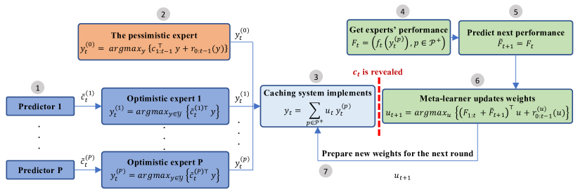
Figure 2: A decision step for the meta-learning policy $\pi_{xc}$. The policy is a combination of experts’ proposals (predictors) according to their priority weights that were learned based on observations that are collected until slot $t$.

1 Input: $C$; $y_{1}\!\in\!\mathcal{Y}$; $\sigma=\sqrt{2}/D_{\mathcal{Y}}$.

2Output: $y_{t}$, $\forall t$.

3for  $t=1,2,\ldots$  do

      4 Observe utility predictions $\{\tilde{c}_{t}^{(p)},p\in\mathcal{P}\}$

      5 Calculate optimistic proposals $\{\!y^{(p)}_{t}\!\}_{p\in\mathcal{P}}$ with (25)

      6 Update $r_{0:t-1}(x)$ using (7)-(8) with $\widetilde{c}_{t}\!=\!0$

      7 Calculate pessimistic proposal $y^{(0)}_{t}$ with (9)

      8 Serve request $q_{t}$ with meta-policy $y_{t}$ from (26)

      9 Observe the utilities of experts’ proposals $F_{t}=\left(f_{t}(y_{t}^{(p)}),p\in\mathcal{P}^{+}\right)$

      10 Set experts’ performance prediction $\tilde{F}_{t+1}\!=\!F_{t}$

      11 Calculate the new weights $u_{t+1}$ using (27)

      

end for

Algorithm 3 Experts Caching ($\pi_{xc}$)

Namely, the caching decision is the convex combination of experts’ proposals according to the weights $u_{t}\!=\!(u^{(p)}_{t},p\in\mathcal{P}^{+})$ selected from the simplex:

$$\Delta_{\mathcal{P}^{+}}=\bigg{\{}u\in[0,1]^{P+1}\bigg{|}\sum_{p\in\mathcal{P}^{+}}=1\bigg{\}},$$

namely:

$$y_{t}=\sum_{p\in\mathcal{P}^{+}}u^{(p)}_{t}\ y^{(p)}_{t}.$$ (26)

Thus, $y_{t+1}$ remains a feasible caching vector, despite being produced by mixing all the experts’ proposals. The mixing weights, $\{u_{t}\}_{t}$, are updated through a new OFTRL step, which is similar to the updates of $\pi_{obc}$ but we use the superscript $(u)$ for the involved parameters to make clear the distinction. In particular, the update is:

$$u_{t+1}=\arg\min_{u\in\Delta_{\mathcal{P}^{+}}}\Big{\{}r_{0:t}^{(u)}(u)-(F_{1:t}+\tilde{F}_{t+1})^{\top}u\Big{\}},$$ (27)

where $F_{t}=\big{(}f_{t}(y_{t}^{(p)}),p\in\mathcal{P}^{+}\big{)}$ is the $t$-slot performance vector for the experts. The regularizers and the respective parameters, in this case, are decided by the following formulas:

$$\!\!r_{0}^{(u)}(x)=\bm{I}_{\Delta_{\mathcal{P}^{+}}}(u),\,\,\,\,r_{t}^{(u)}(x)=\frac{\sigma_{t}^{(u)}}{2}\|u-u_{t}\|^{2},\,\,t\geq 1,$$ (28)

$$\sigma_{1}^{(u)}=\sigma^{(u)}\sqrt{h_{1}^{(u)}},\sigma_{t}^{(u)}=\sigma^{(u)}\left(\sqrt{h_{1:t}^{(u)}}-\sqrt{h_{1:t-1}^{(u)}}\right),\ t\geq 2,$$

$$\text{with}\quad h_{t}^{(u)}=\|F_{t}-\widetilde{F}_{t}\|^{2}.$$

For the predictions of the experts’ performance $\tilde{F}_{t}$, at each time step, we will use expert’s performance of the previous time step:

$$\widetilde{F}_{t} =\left(\widetilde{f}_{t}^{(p)},\ p\in\mathcal{P}^{+}\right)\triangleq\left(f_{t-1}(y_{t-1}^{(p)}),\ p\in\mathcal{P}^{+}\right).$$ (29)

This type of meta-optimism comes for free since, in practice, we expect the predictors to have consistent accuracy across contiguous slots; either accurately due to recently trained model, or poorly due to e.g., distributional shift (see [67] and references therein) hence we can use the previous function. As for the pessimistic expert, its caching decisions do not vary much in consecutive slots (due to using strongly convex regularizers in updating the decisions).

The execution of the policy is summarized in Algorithm 3; and we also include the step-by-step visualization in Fig. 2 so as to facilitate the reader. Namely, we see the sequence of steps where: (1) The Predictors output $\{\tilde{c}_{t}^{(p)},p\in\mathcal{P}\}$; (2) The optimistic experts optimize for the predictions, whereas the pessimistic expert performs an FTRL step; (3) The experts’ proposals are combined via the meta-learner weights; (4) The performance of experts’ proposals is calculated through the revealed request; (5) The meta-learner optimistically sets the next-slot experts’ performance to be the same as the current one; (6) & (7) The meta-learner performs an OFTRL step to calculate and set the weights for the next-slot. And the process repeats for the next slot.

TABLE II: Online caching policies with adversarial guarantees: a summary of the contributions and comparison with literature.

Algorithm	Model and Conditions	Guarantees ($R_{T},V_{T}\leq$ )		Adaptive Learning
		Best case	Worst case
1 ($\pi_{obc}$)	$\bullet$ Bipartite network $\bullet$ Coded files $\bullet$ Predictions	$0$	$O\left(\sqrt{T}\right)$	✓
2 ($\pi_{ec}$)	$\bullet$ Bipartite $\bullet$ Coded files $\bullet$ Predictions $\bullet$ Budget constr.	$O\left(\kappa\sqrt{T}\right),O\left(\kappa T^{\frac{3}{4}}\right)$	$O\left(\!\frac{\kappa}{2}\sqrt{T}\!\right),O\left(\!\frac{\kappa}{2}T^{\frac{3}{4}}\!\right)$	✓
3 ($\pi_{xc}$)	$\bullet$ Bipartite network $\bullet$ Coded files $\bullet$ $P\geq 1$ predictors	​​ $\!\!A_{P}\!\triangleq\!\min_{p\in\mathcal{P}^{+}}\!\left\{\!R_{T}^{(p)}\!\right\}\!\!\!\!$	$2w\sqrt{(P+1)T}\!+\!A_{P}$	✓
[20]	$\bullet$ Single cache $\bullet$ Coded & uncoded files	$O\left(\sqrt{T}\right)$		–
[18]	$\bullet$ Bipartite network $\bullet$ Coded files	$O\left(\sqrt{T}\right)$		–
[21]	$\bullet$ Bipartite network $\bullet$ Coded (single cache) & uncoded	$O\left(\sqrt{T}\right)$		–
[19]	$\bullet$ General graph network $\bullet$ Coded & uncoded files	$O\left(\sqrt{T}\right)$		–
[22]	$\bullet$ Bipartite network $\bullet$ Coded & uncoded files	$O\left(\sqrt{T}\right)$		–

The following theorem bounds the regret, defined as:

$$R^{(xc)}_{T}\!=\sum_{t=1}^{T}\!{c_{t}}^{\top}(y^{\star}-y_{t}),$$

of the proposed meta-learning policy.

Theorem 3.

Algorithm 3 ensures the regret bound: $\displaystyle R^{(xc)}_{T}\!$ $\displaystyle\leq 2\sqrt{\sum_{t=1}^{T}\|F_{t}-{F}_{t-1}\|^{2}}+\min_{p\in\mathcal{P}^{+}}\left\{R_{T}^{(p)}\right\}$ $\displaystyle\leq 2w\sqrt{(P+1)T}+\min_{p\in\mathcal{P}^{+}}\left\{R_{T}^{(p)}\right\}.$

Proof.

We first relate the regret of the combined caching decisions to that of the experts. Then, we can re-use the result of Theorem 1:

$$\!R^{(xc)}_{T}\! =\!\sum_{t=1}^{T}\!\left({c_{t}}^{\top}{y^{\star}}\!-\!{c_{t}}^{\top}\sum_{p\in\mathcal{P}^{+}}u^{(p)}_{t}\ y^{(p)}_{t}\right)=\sum_{t=1}^{T}{c_{t}}\!^{\top}\!{y^{\star}}\!-\!{F_{t}}\!^{\top}\!{u_{t}}$$

$$=\sum_{t=1}^{T}{c_{t}}^{\top}{y^{\star}}-{F_{t}}^{\top}{u^{\star}}+{F_{t}}^{\top}{u^{\star}}-{F_{t}}^{\top}{u_{t}}$$

$$=R_{T}^{(u)}+\min_{p\in\mathcal{P}^{+}}\left\{R_{T}^{(p)}\right\}$$ (30)

where $R_{T}^{(u)}$ is the regret for the weights $u$: $R_{T}^{(u)}=\sum_{t=1}^{T}{F_{t}}^{\top}{u^{\star}}-{F_{t}}^{\top}{u_{t}}$. Note that (30) holds because $u^{\star}\!\!=\!\operatorname*{argmax}_{u}\ {F_{1:t}}\!\!^{\top}\!{u}\!={e^{k}}$, $k=\operatorname*{argmax}_{p}f_{t}(y_{t}^{(p)})$ and $e^{k}$ is standard basis vector. Thus, we have:

$$F_{1:t}^{\top}\ u^{\star}=\max_{p\in\mathcal{P}^{+}}\bigg{\{}\sum_{t=1}^{T}f_{t}(y^{(p)}_{t})\bigg{\}}.$$ (31)

We use the result of Theorem $1$ to bound $R_{T}^{(u)}$:

$$R_{T}^{(u)}\leq\sqrt{2}\Delta_{\mathcal{P}^{+}}\sqrt{\sum_{t=1}^{T}\|F_{t}-\tilde{F}_{t}\|^{2}}\leq 2w\sqrt{(P+1)T},$$ (32)

where the last inequality follows from the simplex diameter ($\sqrt{2}$) and the fact that:

$$\|F_{t}-\tilde{F}_{t}\|^{2}\leq\sum_{p\in\mathcal{P}^{+}}\|(f_{t}(y_{t}^{(p)})-f_{t-1}(y_{t-1}^{(p)}))\|^{2}\leq|\mathcal{P}^{+}|w^{2}$$

i.e., we predicted a miss or a hit, whichever happened at $t-1$, but the opposite happens at $t$. Substituting in (30) gives the bound. ∎

Discussion. A key observation in Theorem 3 is that its bound contains the regret of the best optimistic expert. This yields very improved bounds for $R_{T}^{(xc)}$ whenever there is an optimistic expert that achieves negative regret. For example, if an expert can achieve $R_{T}\!=\!\Theta(-T)$, e.g., because it has a very accurate rec-sys (its recommendations are most-often followed), then the overall regret is $R_{T}^{(xc)}\!=\!O(\sqrt{T})\!-\Theta(-T)$, which becomes strictly negative for large $T$. Moreover, the $O(\sqrt{T})$ term shrinks with more consistent performance of the experts, a condition that is rather expected in practical systems, thus getting us even faster to the regret of the best expert. Nonetheless, since the pessimistic expert exists in the group of experts, the $\min$ term is upper bounded by $O(\sqrt{T})$ and $R_{T}^{(xc)}$ will maintain $O(\sqrt{T})$ regardless of the performance of the optimistic experts.

Since Algorithm XC can work with a single optimistic expert, which is the setup handled by $\pi_{obc}$, it is interesting to compare their bounds. In fact, neither of those algorithms is better in all possible scenarios (regarding request patterns; evolution of utility parameters, etc. see also Sec. 6) than the other; and their relative performance ranking (in terms of utility) depends on the specific problem instance. For example, under worst-case predictions, we have that:

$$R_{T}^{(xc)} \leq 2w\sqrt{(P+1)T}+2w\sqrt{CT}$$

$$\leq 2(\sqrt{2}+\sqrt{C})w\sqrt{T}\qquad\qquad(P=1),$$ (33)

which can be actually better than policy $\pi_{obc}$’s worst-case prediction bound for practical values of the constants $C$.

On the other hand, in cases where inaccurate predictions occur for a certain fraction of the steps $\lceil\alpha T\rceil,0<\alpha<1$ the $\min$ term in the $R_{T}^{(xc)}$ bound might evaluate to the pessimistic expert’s regret since the optimistic experts can suffer linear regrets $R^{(p)}_{T}\leq O(\alpha T)$. For $\pi_{obc}$, the regret will be of the form

$$R_{T} \leq 2\sqrt{C}\sqrt{\sum_{t\in\left[\lceil\alpha T\rceil\right]}\|\tilde{c}_{t}-c_{t}\|}$$

$$\leq 2\sqrt{2C}w\sqrt{\lceil\alpha T\rceil}.$$ (34)

For example, for $\alpha\leq 1/2$, The upper bound in (34) is tighter than that in (33) for all ${C,w}$. Hence, $\pi_{obc}$’s regret can be smaller if in the described case. Overall, the choice between $\pi_{xc}$ and $\pi_{obc}$ in the case of a single predictor depends on the request sequence and the number of steps where predictions fail. Section 6 demonstrates these cases using various scenarios.

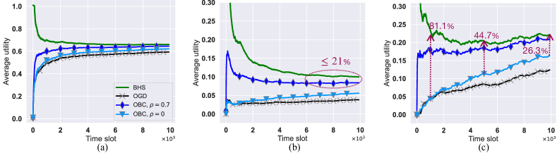
Figure 3: Utility in the single cache model with one rec-sys of different recommendation quality levels (i.e., $\rho$) in (a) Zipf requests with $\zeta=1.1$, (b) YouTube request traces, (c) MovieLens request traces.

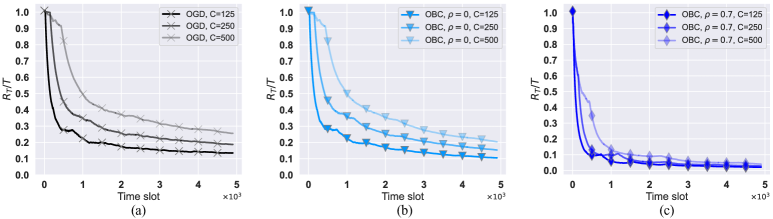
Figure 4: Regret over time in the single cache model with different values of the cache capacity for (a) $\pi_{ogd}$, (b) $\pi_{obc}$ with $\rho=0$, (c) $\pi_{obc}$ with $\rho=0.7$.

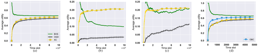
Figure 5: Utility in the single cache model with two rec-sys of recommendation qualities $\rho=2\%$ and $\rho=20\%$, each modeled as an expert within XC, in (a) Zipf requests with $\zeta=1.1$, (b) YouTube request traces, (c) MovieLens request traces. (d) A comparison between $\pi_{obc}$ and $\pi_{xc}$ using one rec-sys of an alternating recommendation quality.

Regarding the extension to caching networks (more than one cache), note that sets $\mathcal{Y}$ and $\mathcal{Z}$ are convex by definition. Also, the set defined by the connectivity constraints (3) is convex (linear constraint in the variable $x$). Recalling that the Cartesian product and the intersection of convex sets is convex, we conclude that the constraint set $\mathcal{X}$ defined in (5), from which the joint caching-routing variable $z$ is selected, remains convex. Finally, as demonstrated earlier, the meta-learner takes the convex combination of the experts proposals, and since each expert proposes a caching-routing configuration $z_{t}^{(p)}\in\mathcal{X}$, the meta caching-routing policy:

$$z_{t+1}=\sum_{p\in\mathcal{P}^{+}}u^{(p)}_{t+1}\ z^{(p)}_{t+1},\quad\quad u^{(p)}_{t+1}\in\Delta_{\mathcal{P}^{+}}$$ (35)

remains a valid one (i.e., $z_{t}\in\mathcal{X},\forall t$). Therefore, indeed, the ideas proposed in this section can be readily applied to bipartite caching networks.

Finally, since we have now presented our algorithms, let us summarize in Table II their main features and revisit how they compare with the state-of-the-art results. For Alg. 1 - 2, the best case refers to the scenario where the request predictions are perfect $\tilde{c}_{t}=c_{t},\forall t$; and the worst case to the scenario where predictions are furthest from the truth $\tilde{c}_{t}=\arg\max_{c}\|c-c_{t}\|,\forall t$. The dependence of the constant factors of the regret bound, denoted with $\kappa$ to facilitate presentation, was made explicit for Alg. 2 where we saw that these constants shrink with the predictions’ accuracy; and the same holds for Alg. 1. For Alg. 3, the best case refers to the scenario where the experts’ predictions are perfect $\tilde{F}_{t}=F_{t},\forall t$; while the worst case arises when $\tilde{F}_{t}=\arg\max_{F}\|F-F_{t}\|,\forall t$. Algorithms that do not leverage predictions in regret analysis (all prior work in caching) have the best and worst case columns merged. We also distinguish between adaptive and static learning rates. While some prior works do employ time-adaptive learning (dynamic steps), as e.g., in [18], none of them adapts the rates (or, equivalently the regularization) to the observed gradients$\{c_{t}\}_{t}$ and/or prediction errors, as we propose here, but instead use the Lipschitz constant $w$, where $\|c_{t}\|\leq w,\forall t$. This leads to looser bounds in most practical cases [58] and, of course, does not allow to benefit from the availability of predictions.

6 Performance evaluation

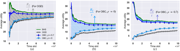
Figure 6: Attained utility in the bipartite model under different recommendation quality levels in (a) Zipf requests with $\zeta=1.1$, (b) YouTube request traces, (c) MovieLens request trace.

We evaluate $\pi_{obc}$, $\pi_{oec}$ and $\pi_{xc}$ under different request patterns and predictions modes; and we benchmark them against $x^{\star}$ and the OGD policy [18] that outperforms other state-of-the-art policies [54, 55]. We observe that when reasonable predictions are available, the proposed policies have an advantage, and under noisy predictions, they still reduce the regret at the same rate with OGD, as proven in the Theorems. First, we compare $\pi_{obc}$ and $\pi_{xc}$ against OGD [18] in the single cache case. We then study $\pi_{obc}$ for the bipartite model and $\pi_{oec}$ with the presence of budget constraints. We consider three requests scenarios, stationary Zipf requests (with parameter $\zeta=1.1$) and two actual request traces: YouTube (YT) [49] and MovieLens (ML) [50]. For predictions, we assume that at each time step, the user follows the recommendation with probability $\rho$ (unknown to the caching system), and we experiment with different $\rho$ values. The full codebase for the proposed policies and experiments is available via GitHub [68].

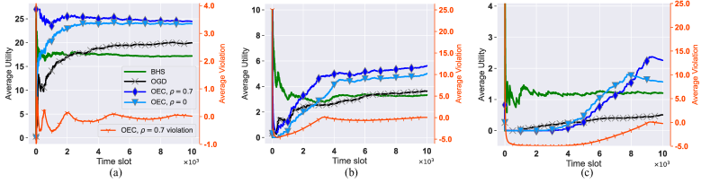
Figure 7: Utility and budget utilization with (a): Zipf requests with $\zeta=1.1$ and (b): YouTube traces (c): MovieLens traces.

Single Cache Scenarios. We set $w=1$ to study the cache hit rate scenario, use a library size of $N=10^{4}$ files, and cache capacity of $C=100$ files. Figures 3.a-c. depict the attained average utility, $\frac{1}{t}\sum_{i=1}^{t}f_{i}(x_{i})$, for each policy and the Best in Hindsight (BHS) cache configuration until that slot, i.e., we find the best in hindsight for each $t$. Note that BHS always achieves utility $1$ initially (first requests to fill the cache). Thus, we cut the y-axis for better presentation in Figures 3.b,c. It can be seen that the accurate predictions (i.e., when users follow the recommendations $70\%$ of the time) pushes the performance of our online caching towards BHS. For example, in 3.b, the utility gap is at most $21\%$ after $t=6k$. At the same time, even when users do not follow the recommendation at all, we still maintain a diminishing regret; the gap in 3.c goes from $81.1\%$ at $t=1k$, to $26.3\%$ at $t=10k$. In Fig. 4, we study the effect of increasing the cache size. Expectedly, the regret increases since the diameter of the decision set also increases. However, with higher prediction quality, this effect is minimized since the regret is proportional to a shrinking error term.

For multiple predictors, we use $\pi_{xc}$. In figures 5.a-c, we evaluate $\pi_{xc}$ with 3 experts: an FTRL expert, and two other optimsitic experts. The first optimistic expert is endowed with a predictor (e.g., a recommendation system) that gets followed with probability $\rho=2\%$. For the other it is $\rho=20\%$. As shown in the plots, $\pi_{xc}$ achieves negative regret on the traces (it outperforms the BHS policy) and converges to the performance of the best expert ($0.20$ utility). This is because in more spread distributions and real request traces, predicting the next request provides great advantage for policies that modify the cache online over the fixed BHS. In the stationary Zipf request pattern, the optimal cache is for the files with top probabilities, which are easily captured by BHS. Thus, BHS policy performs the best. In Fig. 5.d we show the advantages of $\pi_{obc}$ compared to $\pi_{xc}$ with two experts: an FTRL expert and a recommendation-based expert. $\rho$ alternates between $100\%$ and $0\%$ (i.e., requesting the file recommended at a time step $t$, and any other file at $t+1$, and so on). Here, $\pi_{obc}$ outperforms $\pi_{xc}$ since the alternating prediction accuracy induces frequent switching between the two experts in $\pi_{xc}$: the performance of the optimistic expert alternate between $0$ and $1$, while that of pessimistic expert is in the range ($0.55,0.65$). Hence, $\pi_{xc}$ is inclined to place some weight on the prediction expert at one step, only to retract and suffer a greater loss at the following one had it stayed with the full weight on the FTRL expert. Due to the additional regret caused by such frequent switching, $\pi_{obc}$’s regret is $54.8\%$ of $\pi_{xc}$’s. $\pi_{obc}$ also achieves $38.2\%$ of $\pi_{ogd}$’s regret.

Bipartite Networks. We consider next a bipartite graph with $3$ caches and $4$ user locations, where the first two locations are connected with caches $1$ and $2$, and the rest are connected to caches $2$ and $3$. The utility vector is $w_{n}=(1,2,100),\forall i,j$, thus an efficient policy places popular files on cache $3$. This is the setup used in [18] that we adopt here to make a fair comparison. For the zipf scenario, we consider a library of $N=1000$ files and $C=100$. For the traces scenario, files with at least $10$ requests are considered, forming a library of $N=456$ files for the YouTube dataset, and we set $C=50$, and $N=1152$ for the ML dataset, and we increase $C=100$. The location of each request is selected uniformly at random. Similar to the single-cache case, we plot the average utility of the online policies and the best static configuration until each $t$. Recall that the area between a policy and BHS is the average regret of that policy. To avoid clutter, we shade this area for OGD in the first sub-figure, as an example, and for OBC in the next two.

In Fig. 6.a, the effect of good predictions is evident as OBC maintains utility within $5.5\%$ of BHS’s utility after $t=2.5k$. Even when the recommendations are not followed, OBC preserves the sublinear regret, achieving a gap of $30.4\%$ and $8.5\%$ for $t=1k$ and $t=10k$, respectively. Akin patterns appear in the traces scenarios. Namely the similarity between OBC with good predictions and BHS, and the improvement in OBC utility despite the recommendations quality. We also note lower utility scores across all policies due to the more spread request.

Next, we consider the case of budget constraint and evaluate $\pi_{oec}$ for the zipf case, Fig. 7.a, and the two traces: Fig. 7.b, c. The prices at each slot are generated uniformly at random in the normalized range $[0,1]$, and the available budget is generated randomly $b_{t}=\mathcal{N}(0.5,0.05)\times 10$ i.e., enough for approximately $10$ files. Such tight budgets magnify the role of dual variables and allow us to test the constraint satisfaction. The benchmark $x^{\star}$ is computed once for the full time horizon, and its utility is plotted for each $t$. In both scenarios, we note that the constraint violation for all policies is approximately similar, fluctuating during the first few slots and then stabilizing at zero. Hence, we plot it for one case.

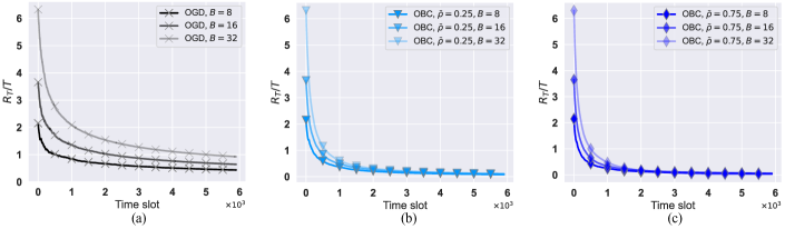
Figure 8: Average regret over time for the single cache, generalized batched requests model for (a) $\pi_{ogd}$, (b) $\pi_{obc}$ with $\bar{\rho}=0.25$, and (c) $\pi_{obc}$ with $\bar{\rho}=0.75$.

Concluding, we find that $\pi_{oec}$ can even outperform the benchmark. This is because the actual request patterns in the traces are not actually adversarial. Also, unlike the benchmark policy, $\pi_{oec}$ is allowed to violate the budget at some time slots, provided that the constraints are eventually satisfied, which occurs either due to strict satisfaction or due to having an ample subsidy at some slots. For example, in the first scenario (Fig. 7.a), the good predictions enable OEC to outperform $x^{\star}$ by $42.2\%$ after observing all requests ($T=5K$). OGD, and OEC with noisy predictions attain utility units improvement of $16.1\%$, $39.3\%$, respectively, over the BHS. We note in Fig.7.b, c the delay in learning due to initially over-satisfied budget constrain. This is a transient effect as the dual variables approach their optimal value. Eventually, the bounds on regret are satisfied. We stress that the algorithms scale for very large libraries $\mathcal{N}$ the only bottleneck in the simulations is finding $x^{\star}$, which involves the horizon $T$; this is not required in real systems.

Computational Complexity. Note that the OFTRL update (e.g., (9)) is either a linear program in case $r_{t}(\cdot)=0,\forall t$, or a quadratic program otherwise. In the former case, the solution is finding the top $C$ most requested files. This can be done through a simple ordering operation whose worst-case complexity is linear in the dimension of the decision variable (e.g., $O(N\log(N)$ for each cache). If, however, we have regularization terms, then the resulting quadratic program can be solved in closed form in $\mathbb{R}$. Then, for the projection to the feasible set $\mathcal{X}$, we can use specialized projection algorithms for the capped simplex (the capacity constraints for each cache) whose worst-case complexity is still polynomial in the dimension (i.e., $O(N^{2})$)[69].

The above discussion is a worst-case one. In practice, we use the fact that we repeatedly solve similar optimization problems at each time step (the update step differs by adding one linear term and one quadratic term). Thus, the solution in a step can be used as an initial point for the following one. We note that the experimental running times are significantly less than the worst-case ones, as can be seen in Fig. 9 and Fig. 10. In these figures, these simulations were done using CVXPY $1.2$ package with Python $3.10$ running on an Apple M1 Pro Chip and 16GB of RAM. The differences between OGD and the optimistic one is due to the difference in the update problem structure (lazy vs. greedy projection).

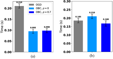
Figure 9: Average time consumed per decision step in the bipartite network configuration and the ML Dataset ($N=1152$, $C=100$, $|\mathcal{I}|=4$, $|\mathcal{J}|=3$) with (a) pre-reserved storage ($\pi_{obc}$), and (b) elastic storage ($\pi_{oec}$).

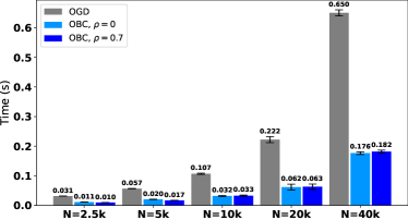
Figure 10: Average time consumed per decision step in the single cache configuration and stationary requests with different library sizes $N$. The sample size is $T=10k$

Batched Requests. As mentioned in the discussion of the system model, as well as that of Theorem 1, our assumption on the request model (one request per time slot) is for technical ease of analysis. The main feature of the proposed policies, which is having $R_{T}\propto O({\sqrt{\sum_{t=1}^{T}\|c_{t}-\widetilde{c}_{t}\|}})$, remains valid when the request model is batched (i.e., processing $B$ requests per time slot). However, the upper bound (not necessarily the regret) will be scaled accordingly since the diameter of the decision set will now increase. Namely, following the same steps in the proof of Theorem. 1 (after (14)), instead of $D_{\mathcal{X}}=2(JC+1)$, we would have $D_{\mathcal{X}}=2(JC+B)$. Fig. 8 shows experimentally how the batch size affects the regret. In this experiment, we introduce a new parameter, $\bar{\rho}$, which denotes the percentage of requests correctly predicted out of the total $B$. We note in these experiments that with better predictions, the effect is amortized since the term $\sqrt{\sum_{t=1}^{T}\|c_{t}-\widetilde{c}_{t}\|}$ remains small.

7 Conclusions

The problem of online caching is timely with applications that extend beyond content delivery to edge computing and in fact to any dynamic placement problem with Knapsack-type constraints. This work proposes a new suite of caching policies that leverage predictions obtained from content recommendations, and possibly other forecasters, to minimize the caching regret w.r.t an ideal (yet unknown) benchmark cache configuration. As recommender systems permeate online content viewing platforms, such policies can play an essential role in optimizing caching efficacy. We identified and built upon this new connection between caching and recommender systems. The proposed algorithmic framework is scalable and robust to the quality of recommendations and the possible variations of network state and the request sequences, which can even be decided by an adversary. The achieved bounds improve upon the previously known caching regret performance, see [18, 19, 20, 21] and references therein. Finally, we believe this work opens new research directions both in terms of caching, e.g., pursuing the design of optimistic policies for uncoded caching; and in terms of resource scheduling in pertinent network and mobile computing problems using untrusted sources of optimism, i.e., predictors of unknown or varying accuracy.

References

- [1] N. Mhaisen, G. Iosifidis, and D. Leith, “Online Caching with Optimistic Learning,” 2022. [Online]. Available: https://arxiv.org/abs/2202.10590
- [2] G. S. Paschos, G. Iosifidis, M. Tao, D. Towsley, and G. Caire, “The Role of Caching in Future Communication Systems and Networks,” IEEE J. Select. Areas Commun., vol. 36, no. 6, pp. 1111–1125, 2018.
- [3] L. A. Belady, “A study of Replacement Algorithms for a Virtual-Storage Computer,” IBM Systems Journal, vol. 5, no. 2, pp. 78–101, 1966.
- [4] C. Aggarwal, J. L. Wolf, and P. S. Yu, “Caching on the World Wide Web,” Trans. Knowledge Data Eng., vol. 11, no. 1, pp. 94–107, 1999.
- [5] J. Kangasharju, J. Roberts, and K. Ross, “Object Replication Strategies in Content Distribution Networks,” Computer Communications, vol. 25, no. 4, pp. 376–383, 2002.
- [6] K. Shanmugam, N. Golrezaei, A. G. Dimakis, A. F. Molisch, and G. Caire, “Femtocaching: Wireless Content Delivery Through Distributed Caching Helpers,” IEEE Trans. Inform. Theory, vol. 59, no. 12, pp. 8402–8413, 2013.
- [7] N. Golrezaei, A. F. Molisch, A. G. Dimakis, and G. Caire, “Femtocaching and Device-to-device Collaboration: A New Architecture for Wireless Video Distribution,” IEEE Commun. Mag., vol. 51, no. 4, pp. 142–149, 2013.
- [8] D. D. Sleator and R. E. Tarjan, “Amortized Efficiency of List Update and Paging Rules,” Commun. ACM, vol. 28, no. 2, pp. 202–208, 1985.
- [9] P. R. Jelenković and X. Kang, “Characterizing the Miss Sequence of the LRU Cache,” SIGMETRICS Perform. Eval. Rev., vol. 36, no. 2, pp. 119–121, 2008.
- [10] D. Lee, J. Choi, J.-H. Kim, S. H. Noh, S. L. Min, Y. Cho, and C. S. Kim, “On the Existence of a Spectrum of Policies That Subsumes the Least Recently Used (LRU) and Least Frequently Used (LFU) Policies,” SIGMETRICS Perform. Eval. Rev., vol. 27, no. 1, pp. 134–143, 1999.
- [11] S. Traverso, M. Ahmed, M. Garetto, P. Giaccone, E. Leonardi, and S. Niccolini, “Temporal Locality in Today’s Content Caching: Why It Matters and How to Model It,” SIGCOMM Comput. Commun. Rev., vol. 43, no. 5, pp. 5–12, 2013.
- [12] F. Olmos, B. Kauffmann, A. Simonian, and Y. Carlinet, “Catalog dynamics: Impact of content publishing and perishing on the performance of a LRU cache,” in Proc. of ITC, 2014.
- [13] M. Leconte, G. Paschos, L. Gkatzikis, M. Draief, S. Vassilaras, and S. Chouvardas, “Placing Dynamic Content in Caches with Small Population,” in Proc. of IEEE INFOCOM, 2016.
- [14] S.-E. Elayoubi and J. Roberts, “Performance and Cost Effectiveness of Caching in Mobile Access Networks,” in Proc. of ICN, 2015.
- [15] S. O. Somuyiwa, A. György, and D. Gündüz, “A Reinforcement-Learning Approach to Proactive Caching in Wireless Networks,” IEEE J. Select. Areas Commun., vol. 36, no. 6, pp. 1331–1344, 2018.
- [16] A. Sadeghi, F. Sheikholeslami, and G. B. Giannakis, “Optimal and Scalable Caching for 5G Using Reinforcement Learning of Space-Time Popularities,” IEEE J. Select. Areas Commun., vol. 12, no. 1, pp. 180–190, 2018.
- [17] S. Geulen, B. Vöcking, and M. Winkler, “Regret Minimization for Online Buffering Problems Using the Weighted Majority Algorithm,” in Proc. of COLT, 2010.
- [18] G. S. Paschos, A. Destounis, L. Vigneri, and G. Iosifidis, “Learning to Cache With No Regrets,” in Proc. of IEEE INFOCOM, 2019.
- [19] Y. Li, T. Si Salem, G. Neglia, and S. Ioannidis, “Online Caching Networks with Adversarial Guarantees,” Proc. ACM Meas. Anal. Comput. Syst., vol. 5, no. 3, 2021.
- [20] T. Si Salem, G. Neglia, and S. Ioannidis, “No-Regret Caching via Online Mirror Descent,” in Proc. of ICC, 2021.
- [21] R. Bhattacharjee, S. Banerjee, and A. Sinha, “Fundamental Limits on the Regret of Online Network-Caching,” Proc. ACM Meas. Anal. Comput. Syst., vol. 4, no. 2, 2020.
- [22] D. Paria and A. Sinha, “LeadCache: Regret-Optimal Caching in Networks,” in Proc. of NeurIPS, 2021.
- [23] C. A. Gomez-Uribe and N. Hunt, “The Netflix Recommender System: Algorithms, Business Value, and Innovation,” ACM Trans. Manage. Inf. Syst., vol. 6, no. 4, 2016.
- [24] X. Amatriain, “Building Industrial-Scale Real-World Recommender Systems,” in Proc. of RecSys, 2012.
- [25] L. E. Chatzieleftheriou, M. Karaliopoulos, and I. Koutsopoulos, “Jointly Optimizing Content Caching and Recommendations in Small Cell Networks,” IEEE Trans. Mobile Comput., vol. 18, no. 1, pp. 125–138, 2019.
- [26] Y. Fu, Q. Yu, T. Q. S. Quek, and W. Wen, “Revenue Maximization for Content-Oriented Wireless Caching Networks (CWCNs) With Repair and Recommendation Considerations,” IEEE Trans. Wireless Commun., vol. 20, no. 1, pp. 284–298, 2021.
- [27] M. Sheng, W. Teng, X. Chu, J. Li, K. Guo, and Z. Qiu, “Cooperative Content Replacement and Recommendation in Small Cell Networks,” IEEE Trans. Wireless Commun., vol. 20, no. 3, pp. 2049–2063, 2021.
- [28] T. Giannakas, P. Sermpezis, and T. Spyropoulos, “Network friendly recommendations: Optimizing for long viewing sessions,” IEEE Trans. on Mobile Comput., 2021.
- [29] Y. Fu, Y. Zhang, A. Wong, and T. Q. Quek, “Revenue maximization: The interplay between personalized bundle recommendation and wireless content caching,” IEEE Trans. on Mobile Comput., 2022.
- [30] M. Zinkevich, “Online Convex Programming and Generalized Infinitesimal Gradient Ascent,” in Proc. of ICML, 2003.
- [31] E. Hazan, “Introduction to Online Convex Optimization,” 2019. [Online]. Available: https://arxiv.org/abs/1909.05207
- [32] A. Antoniadis, C. Coester, M. Elias, A. Polak, and B. Simon, “Online Metric Algorithms with Untrusted Predictions,” in Proc. of ICML, 2020.
- [33] T. Lykouris and S. Vassilvtiskii, “Competitive Caching with Machine Learned Advice,” in Proc. of ICML, 2018.
- [34] L. Andrew, S. Barman, K. Ligett, M. Lin, A. Meyerson, A. Roytman, and A. Wierman, “A tale of two metrics: Simultaneous bounds on competitiveness and regret,” in Proc. of COLT, 2013.
- [35] e. a. O. Dekel, “Online Learning with a Hint,” in Proc. of NeurIPS, 2017.
- [36] A. Bhaskara, A. Cutkosky, R. Kumar, and M. Purohit, “Online Learning with Imperfect Hints,” in Proc. of ICML, 2020.
- [37] A. Rakhlin and K. Sridharan, “Optimization, Learning, and Games with Predictable Sequences,” in Proc. of NeurIPS, 2013.
- [38] M. Mohri and S. Yang, “Accelerating Online Convex Optimization via Adaptive Prediction,” in Proc. of AISTATS, 2016.
- [39] S. Shalev-Shwartz and Y. Singer, “A Primal-Dual Perspective of Online Learning Algorithms,” Mach. Learn., vol. 69, no. 2-3, pp. 115–142, 2007.
- [40] A. Sadeghi, F. Sheikholeslami, A. G. Marques, and G. B. Giannakis, “Reinforcement Learning for Adaptive Caching With Dynamic Storage Pricing,” IEEE J. Select. Areas Commun., vol. 37, no. 10, pp. 2267–2281, 2019.
- [41] J. Kwak, G. Paschos, and G. Iosifidis, “Dynamic Cache Rental and Content Caching in Elastic Wireless CDNs,” in Proc. of WiOpt, 2018.
- [42] E. Nygren, R. K. Sitaraman, and J. Sun, “The Akamai Network: A Platform for High-Performance Internet Applications,” SIGOPS Oper. Syst. Rev., vol. 44, no. 3, pp. 2–19, 2010.
- [43] T. Chen, Q. Ling, and G. B. Giannakis, “An Online Convex Optimization Approach to Proactive Network Resource Allocation,” IEEE Trans. Signal Processing, vol. 65, no. 24, pp. 6350–6364, 2017.
- [44] N. Liakopoulos, A. Destounis, G. Paschos, T. Spyropoulos, and P. Mertikopoulos, “Cautious Regret Minimization: Online Optimization with Long-Term Budget Constraints,” in Proc. of ICML, 2019.
- [45] V. Valls, G. Iosifidis, D. Leith, and L. Tassiulas, “Online Convex Optimization with Perturbed Constraints: Optimal Rates against Stronger Benchmarks,” in Proc. of AISTATS, 2020.
- [46] X. Yi, X. Li, L. Xie, and K. H. Johansson, “Distributed Online Convex Optimization With Time-Varying Coupled Inequality Constraints,” IEEE Trans. Signal Processing, vol. 68, pp. 731–746, 2020.
- [47] Z. Shen, K. Yang, Z. Xi, J. Zou, and W. Du, “Deepapp: A deep reinforcement learning framework for mobile application usage prediction,” IEEE Trans. on Mobile Comput., 2021.
- [48] J. B. Schafer, J. A. Konstan, and J. Riedl, “Meta-Recommendation Systems: User-Controlled Integration of Diverse Recommendations,” in Proc. of CIKM, 2002.
- [49] M. Zink, K. Suh, Y. Gu, and J. Kurose, “Characteristics of YouTube Network Traffic at a Campus Network - Measurements, Models, and Implications,” Comput. Netw., vol. 53, no. 4, pp. 501–514, 2009.
- [50] F. M. Harper and J. A. Konstan, “The MovieLens Datasets: History and Context,” ACM Trans. Interact. Intell. Syst., vol. 5, no. 4, 2015.
- [51] G. Paschos, G. Iosifidis, and G. Caire, “Cache Optimization Models and Algorithms,” FnT in Communications and Information Theory, vol. 16, no. 3–4, pp. 156–345, 2020.
- [52] Georgios S. Paschos, Ejder Bastug, Ingmar Land, Giuseppe Caire, and Merouane Debbah, “Wireless Caching: Technical Misconceptions and Business Barriers,” IEEE Commun. Mag., vol. 54, no. 8, pp. 16–22, 2016.
- [53] X. Huang, S. Zhao, X. Gao, Z. Shao, H. Qian, and Y. Yang, “Online User-AP Association with Predictive Scheduling in Wireless Caching Networks,” IEEE Trans. Mobile Comput., 2020.
- [54] A. Giovanidis and A. Avranas, “Spatial Multi-LRU Caching for Wireless Networks with Coverage Overlaps,” SIGMETRICS Perform. Eval. Rev., vol. 44, no. 1, pp. 403–405, 2016.
- [55] E. Leonardi and G. Neglia, “Implicit Coordination of Caches in Small Cell Networks Under Unknown Popularity Profiles,” IEEE J. Select. Areas Commun., vol. 36, no. 6, pp. 1276–1285, 2018.
- [56] D. Tsigkari and T. Spyropoulos, “User-centric Optimization of Caching and Recommendations in Edge Cache Networks,” in Proc. of WoWMoM, 2020.
- [57] T. Si Salem, G. Neglia, and S. Ioannidis, “No-regret caching via online mirror descent,” 2021. [Online]. Available: https://arxiv.org/abs/2101.12588
- [58] H. B. McMahan, “A Survey of Algorithms and Analysis for Adaptive Online Learning,” J. Mach. Learn. Res., vol. 18, no. 1, pp. 3117–3166, 2017.
- [59] A. Beck, First-Order Methods in Optimization. SIAM-Society for Industrial and Applied Mathematics, 2017.
- [60] F. Orabona, “A Modern Introduction to Online Learning,” 2019. [Online]. Available: https://arxiv.org/abs/1912.13213
- [61] P. Auer, N. Cesa-Bianchi, and C. Gentile, “Adaptive and Self-Confident On-Line Learning Algorithms,” Journal of Computer and System Sciences, vol. 64, no. 1, pp. 48–75, 2002.
- [62] G. S. Paschos, A. Destounis, and G. Iosifidis, “Online Convex Optimization for Caching Networks,” IEEE/ACM Trans. Networking, vol. 28, no. 2, pp. 625–638, 2020.
- [63] “Amazon Elastic CDN Service - ElastiCache.” [Online]. Available: https://aws.amazon.com/elasticache/
- [64] Juniper Networks, “The Elastic CDN Solution,” Solution Brief, Dec. 2014. [Online]. Available: https://www.juniper.net/assets/kr/kr/local/pdf/solutionbriefs/3510532-en.pdf
- [65] S. Mannor, J. N. Tsitsiklis, and J. Y. Yu, “Online Learning with Sample Path Constraints,” J. Mach. Learn. Res., vol. 10, pp. 569–590, 2009.
- [66] D. Anderson and D. J. Leith, “Learning the best expert efficiently.” [Online]. Available: https://arxiv.org/abs/1911.04307
- [67] Y. Zhang, F. Feng, C. Wang, X. He, M. Wang, Y. Li, and Y. Zhang, “How to Retrain Recommender System? A Sequential Meta-Learning Method,” in Proc. of SIGIR, 2020.
- [68] N. Mhaisen, “online-caching.” [Online]. Available: https://github.com/Naram-m/online-caching
- [69] W. Wang and C. Lu, “Projection onto the capped simplex,” 2015. [Online]. Available: https://arxiv.org/abs/1503.01002