Unsupervised Domain Adaptation for Cardiac Segmentation: Towards Structure Mutual Information Maximization

Abstract

Unsupervised domain adaptation approaches have recently succeeded in various medical image segmentation tasks. The reported works often tackle the domain shift problem by aligning the domain-invariant features and minimizing the domain-specific discrepancies. That strategy works well when the difference between a specific domain and between different domains is slight. However, the generalization ability of these models on diverse imaging modalities remains a significant challenge. This paper introduces UDA-VAE++, an unsupervised domain adaptation framework for cardiac segmentation with a compact loss function lower bound. To estimate this new lower bound, we develop a novel Structure Mutual Information Estimation (SMIE) block with a global estimator, a local estimator, and a prior information matching estimator to maximize the mutual information between the reconstruction and segmentation tasks. Specifically, we design a novel sequential reparameterization scheme that enables information flow and variance correction from the low-resolution latent space to the high-resolution latent space. Comprehensive experiments on benchmark cardiac segmentation datasets demonstrate that our model outperforms previous state-of-the-art qualitatively and quantitatively. The code is available at https://github.com/LOUEY233/Toward-Mutual-Information

1 Introduction

Deep learning-based methods have recently achieved promising results on various medical image processing tasks, such as detection [23, 35] and segmentation [29, 7]. Indeed, deep learning approaches can generalize effectively when the training and testing images are from the same modality (i.e., same distribution), approaching or surpassing human-level performance.

However, some researchers [15, 32] have shown that well-trained models do not perform well when the testing images come from a different statistical distribution from the training images. This domain shift problem is common in real-world medical diagnosis since medical images at various steps of the clinical procedure are often obtained with different physical properties [6]. For instance, Magnetic Resonance Imaging (MRI) and Computed Tomography (CT) play complementary roles in cardiac disease diagnosis while also exhibiting different appearances (See Fig. 1). That difference post challenges for analyzing the MRI and CT images in clinical diagnosis.

One plausible solution is to obtain manual annotations for both the MRI and the CT images from medical experts. However, such a procedure is prohibitively time-consuming. (e.g., manual cardiac operations from MRI/CT consumes 2-4 hours [39]). Unsupervised Domain adaptation (UDA), which automatically transfers knowledge from the source domain to the target domain (e.g., MRI to CT) without paired images, is an interesting idea.

For UDA with medical image segmentation, the source medical image with the ground truth segmentation is denoted as the source domain, whereas the target medical image without the ground truth segmentation is referred to as the target domain. Generally, the reported works such as [6, 5] align the source domain and the target domain by learning the domain-invariant features and minimizing the domain-specific discrepancies.

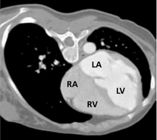
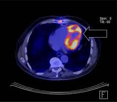
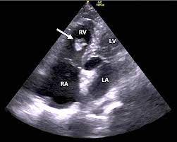
Figure 1: Four types of Cardiac Imaging. From left to right: Computerized Tomography (CT), Magnetic Resonance Imaging (MRI), Positron Emission Tomography (PET), and Ultrasound (US).[27] Each type has significant difference with others in terms of color, contrast, structure, artifacts, and the edge information.

One popular research direction is to combine UDA with a GAN-based strategy, as GAN [9] and its derivatives [38, 14] have exhibited remarkable unsupervised domain adaption ability. In the GAN-based UDA approach, the domain-invariant latent space features can be implicitly learned via adversarial learning during the min-max game between the generator and the discriminator. GAN-based approaches [37, 2, 22] have recently gained widespread acceptance in medical image analysis, outperforming prior Convolutional Neural Network (CNN) methods such as [6, 5] on cardiac segmentation tasks [41, 37]. However, when we have a dataset (e.g., [40]) with extremely diverse imaging modalities and scanning methods, GAN-based approaches often fail to converge to the Nash Equilibrium [12, 16, 17, 34].

Recently, researchers [25, 10, 33, 34] in UDA with medical imaging have turned to Variational Autoencoder (VAE) [19] as the backbone due to their training stability at domain adaptation tasks at diverse imaging modalities [28, 34] and their ability to handle scarce data in the target domain [25, 10]. These VAE-based methods usually perform posterior inference for the latent space variables using the normal distribution. That property allows it to consistently bridge two domains (i.e., source and target domain) towards standard and parameterized latent space variables [34].

Despite VAE-based methods’ excellent domain adaptation ability at challenging benchmark cardiac segmentation datasets (e.g., [40]), two crucial factors restrain their learning capability. Firstly, VAE-based methods like UDA-VAE [34] introduce a separate image reconstruction stage, aiming to regularize the latent space towards normal distribution. Although this strategy could explicitly minimize the domain discrepancy, the information from the reconstructed output cannot be directly delivered to the segmentation. Secondly, VAE-based approaches like CFDNet [33] utilize parallel reparameterization for latent space with different resolutions. The separation of low-resolution latent space and high-resolution latent space in U-Net-like architecture will potentially exaggerate the domain shift problem [36] and, therefore, degrade the model performance.

In this work, we propose a new framework, dubbed UDA-VAE++, that can well address unsupervised domain adaptation in cardiac image segmentation with diverse imaging modalities. Firstly, we leverage a U-Net backbone to extract the multi-scale features from unpaired images from the source and the target domain. The output at each encoder stair enters variational reasoning, followed by our sequential reparametrization design. That sequential design enables the network to transfer knowledge from low-resolution latent space to high-resolution latent space and constrains the encoded output according to standard normal distribution. A segmentation block follows the reparametrization operation at each level, and the segmentation output will be passed into a reconstruction block. Finally, we conduct mutual information (global, local, prior) estimation and maximization for the segmentation output and the reconstruction to evaluate the compact loss function lower bound.

The main contributions of this paper are highlighted as follows:

• We deduce a compact loss function lower bound in which each term is orthogonal, discovering a new mutual information term.

• We design a novel, plug-and-play style, Structure Mutual Information Estimation (SMIE) block. This design enables an efficient mutual information estimate for the reconstruction output and the segmentation output, making the reconstruction and segmentation tasks mutually beneficial.

• We convert parallel reparameterization to sequential reparameterization, allowing information flow and variance correction from the low-resolution latent space to the high-resolution latent space after variational reasoning.

• We conduct extensive experiments to demonstrate that the proposed method surpasses previous state-of-the-arts on benchmark cardiac segmentation datasets qualitatively and quantitatively.

2 Related Work

2.1 Unsupervised Domain Adaptation

Unsupervised Domain Adaptation (UDA) has been widely used for biomedical image segmentation tasks. The early works [6] and [5] leverage unsupervised domain adaptation with adversarial training for multi-modal biomedical image segmentation. Specifically, both papers utilize a plug-and-play domain adaptation module to align the features in the source and the target domain.

Due to the promising generalization ability of Generative Adversarial Network (GAN) [9], recent research has begun to incorporate GAN in UDA for biomedical image segmentation. For example, [37] utilizes CycleGAN [38] with a shape-consistency loss to realize cross-domain translation between CT and MRI images. SIFA [2] presents a synergistic domain alignment at both image-level and feature-level using the adversarial learning of CycleGAN to exploit domain-invariant characteristics. DUDA [22] further incorporates a cross-domain consistency loss to improve the segmentation performances.

Another faithful research direction is to use Variational Autoencoder (VAE) [19]. That strategy is advantageous when there are few images in the target domain. For instance, [25] follows the few-shot learning strategy, integrating a VAE-based feature prior to matching with adversarial learning to exploit the domain-invariant features. FUDA [10] further incorporates Random Adaptive Instance Normalization to explore diverse target styles where there is only one unlabeled image in the target domain. The recent work CFDNet [33] proposes an effective metric, dubbed CF Distance, which enables explicit domain adaptation with image reconstruction and prior distribution matching. Another work UDA-VAE [34] goes even further: it drives the latent space of the source and target domains towards a common, parameterized variational form following Gaussian Distribution.

Compared with previous UDA approaches, our method is the first that sequentially integrates multi-scale latent space features. That design enables our network to effectively minimize the domain-specific discrepancy according to the information flow from the low-resolution latent space to the high-resolution latent space.

2.2 Mutual Information Neural Estimation

Mutual Information Neural Estimation (MINE) is first introduced in [1], where the author utilizes gradient descent algorithms over neural networks to approximate the mutual information between continuous random variables. Based upon MINE, Deep InfoMax (DIM) [13] explores unsupervised visual representation learning by maximizing the mutual information for the network input and the encoded output under statistical constrain. A recent work [3] utilizes MINE to address the domain shift problem in unsupervised domain adaptation. Specifically, that paper integrates network predictions and local features into global features by simultaneously maximizing the mutual information.

Recently, MINE has been applied in biomedical image processing tasks. For example, based on MINE, [31] maximizes the mutual information between source and fused images from Multiview 3-D Echocardiography. [30] tackle the challenging unsupervised multimodal brain image segmentation task by estimating the mutual information using a lightweight convolutional neural network.

Different from previous MINE approaches, our framework is the first that conducts mutual information estimation and maximization with both image reconstruction and image segmentation. Our unique design enables image reconstruction and image segmentation to be mutually beneficial during model learning.

	Symbols	Description
	$S$	Source domain
	$T$	Target domain
	$z$	Latent variable
	$x$	Input image data point
	$p_{\theta}()$	PDF of variables with parameter $\theta$
	$q_{\phi}()$	Neural network with parameter $\phi$
	$D(\phi_{S},\phi_{T})$	Domain distance between source and target
	$\hat{y}$	Predicted segmentation
	$y$	Ground truth segmentation
	$R_{S}$	Reconstructed image in the source domain
	$R_{T}$	Reconstructed image in the target domain
	$D_{KL}$	KL Divergence
	$\epsilon$	Reconstruction error
	$H$	Entropy

Table 1: Preliminary for Important Symbols

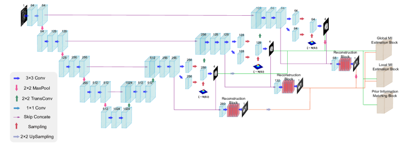
Figure 2: The Model Architecture of UDA-VAE++. The backbone of UDA-VAE++ is U-Net (blue boxes) with three scales of variational blocks. The green line refers to the concatenation of the segmentation output, whereas the orange line indicates the concatenation of the reconstruction output. The reconstruction blocks (red boxes) contain seven convolution layers. The grey box refers to the MI estimation block detailed in Fig. 4

3 Methodology

In this section, we will discuss our UDA-VAE++ workflow, explain the proposed structure mutual information estimation block, and display the loss functions.

3.1 UDA-VAE++ Model Workflow

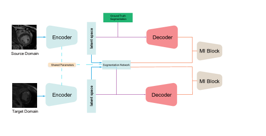
Figure 3: The workflow for Unsupervised Domain Adaptation. The image from the source and target domain will first be encoded in the shared parameters downsampling part of the U-Net backbone. Next, each scale output will go through the same segmentation network. In the source domain, the ground truth segmentation masks combining the variables in latent space will be reconstructed by the upsampling part of U-Net. The MI block will maximize the mutual information of the segmentation output and the reconstruction output.

As shown in Fig. 2, we use U-Net [29] as our backbone due to its remarkable success in medical image segmentation. Firstly, The network performs four downsamplings. Each of the downsampling operations uses two convolutional layers. Secondly, the network uses upsampling symmetrically with skip connection. We then obtain a multi-scale encoding output with channels of 256, 128, 64, and image sizes of 40$\times$40, 80$\times$80, 160$\times$160, respectively. Each encoding output will be followed by variational reasoning [19, 21]. Using the reparameterization trick [19] with the latent mean variable, the latent log variance variable, and the standard normal distribution, we obtain three latent variables $z_{1},z_{2},z_{3}$. After that, We use a single convolutional layer to obtain the predicted segmentation $\hat{y}$.

Finally, we leverage a fully convolutional network with 7 layers for image reconstruction. The input for the source domain includes the ground truth segmentation $y$ and the latent variable $z$, whereas the input for the target domain is the predicted segmentation $\hat{y}$.

3.2 Structure Mutual Information Estimation

In this subsection, we aim to estimate the mutual information between the segmentation outcome $\hat{y}$ and the reconstruction output $R$ in the source and target domains. The mutual information can be formulated as:

$$\widehat{\mathcal{I}}\left(\hat{y};R\right)=D_{KL}\left(\mathbb{P}_{\hat{y}R}\|\mathbb{P}_{\hat{y}}\otimes\mathbb{P}_{R}\right)$$ (1)

The KL divergence between joint distribution $\mathbb{P}_{\hat{y}R}$ and marginal distribution $\mathbb{P}_{\hat{y}}\otimes\mathbb{P}_{R}$ can be written as its dual representation[4] as below:

$$D_{KL}(\mathbb{P}_{\hat{y}R}\|\mathbb{P}_{\hat{y}}\otimes\mathbb{P}_{R})=\sup_{T:\Omega\rightarrow\mathbb{R}}(\mathbb{E}_{\mathbb{P}_{\hat{y}R}}[T]-\log\left(\mathbb{E}_{\mathbb{P}_{\hat{y}}\otimes\mathbb{P}_{R}}\left[e^{T}\right]\right))$$ (2)

where T is the set of all possible neural network.

Inspired by [13], we are interested in automatically maximizing the mutual information rather than manually obtaining the exact value for mutual information. The mutual information maximization process can be formulated as:

$$\widehat{\mathcal{I}}\left(\hat{y};R\right)=\mathbb{E}_{\mathbb{P}_{\hat{y}R}}\left[-\operatorname{sp}\left(-T\left(\hat{y},R\right)\right)\right]-\mathbb{E}_{\mathbb{P}_{\hat{y}}\otimes\mathbb{P}_{R}}\left[\operatorname{sp}\left(T\left(\hat{y},R^{\prime}\right)\right)\right]$$ (3)

where $R^{\prime}$ is an input sampled from $R$, and $\operatorname{sp}(z)=\log\left(1+e^{z}\right)$ is the softplus function.

The next step is to estimate the joint and marginal distribution of $\hat{y}$ and $R$ using contrastive learning. First, we design three estimators in the MI block [13]. The original paired $R$ and $\hat{y}$ serve as the anchor and the positive point, respectively. We then shuffle $R$ randomly to obtain the negative point. To fuse the data together, we upsample the 40$\times$40 feature map and downsample the 160$\times$160 feature map. Before entering the estimator block, the anchor and negative point will go through two convolutional layers, whereas the positive point will go through three convolutional layers.

For the Global MI Estimation block, we concatenate the positive points with anchor and negative points, pushing the anchor away from the negative points and pulling the anchor towards the positive point. For the Local MI Estimation block, we extract the high-level semantics using fully connected layers. Next, we concatenate the semantic information with the positive point to acquire the locality information, followed by two convolutional layers for contrastive learning.

Finally, motivated by [13, 3], we adopt the prior matching [24] strategy to constrain the visual representations according to standard normal distribution. Specifically, in the prior information estimation block, the positive point will go through fully connected layers and output the prior information.

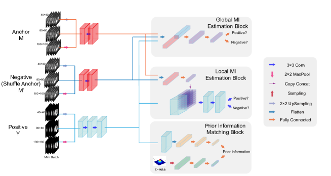
Figure 4: The architecture of Structure Mutual Information Estimation (SMIE) block. We use the reconstruction image as anchor, the shuffle reconstructed images as negative points, and the segmented image as positive points. The Global & Local Mutual Information (MI) Estimation Block follows contrastive learning schemes to maximize mutual information, whereas the prior information matching block align the positive point with the standard normal distribution. Finally, the sum of the outputs score from these three blocks serves as the loss function for $\mathcal{L}_{MI}$.

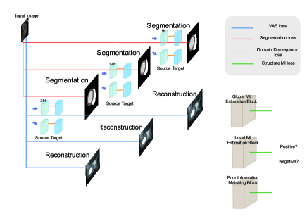
Figure 5: The loss function of the proposed method. The blue line refers to the reconstruction loss. The red line indicates the segmentation loss between the predicted segmentation and ground truth segmentation. The orange line illustrates the domain discrepancy loss in the latent space. The green line refers to the structure mutual information loss.

3.3 Loss function

For the segmentation part, we aim to maximize the joint log-likelihood $\log p_{\theta_{S}}(x,y)$ of the dataset.

Theorem 1

$$\log p_{\theta_{S}}(x,y)$$ (4)

$$\geq \left(\mathcal{\epsilon}+\widehat{\mathcal{I}}_{q\phi_{S}}(x,y,z)-H_{q\phi_{S}}(z)+\log\frac{p_{\theta_{S}}(x,y)}{q_{\phi_{S}}(x,y)}\right)$$

$$-D_{KL}\left(q_{\phi_{S}}(z\mid x)\|p_{\theta_{S}}(z)\right)$$

$$+E_{q_{\phi_{S}}(z\mid x)}[\log p_{\theta_{S}}(x\mid y,z)]$$

$$+E_{q_{\phi_{S}}(z\mid x)}[\log p_{\theta_{S}}(y\mid z)]$$

where $\epsilon,H_{q\phi_{S}(z)},\log\frac{p_{\theta_{S}}(x,y)}{q_{\phi_{S}}(x,y)}$ are all constant.

Proof 3.1

Detailed proof will be in the supplementary material.

For the domain discrepancy loss, we minimize it explicitly as the latent space obeys normal distribution.
Therefore, our loss function (Fig. 5) contains structure mutual information estimation loss $\mathcal{L}_{MI}$(Eq.4 line 1) reconstruction loss $\mathcal{L}_{recon}$(Eq.4 line 2,3), segmentation loss $\mathcal{L}_{seg}$(Eq.4 line 4), and domain discrepancy loss $\mathcal{L}_{D}$.

3.3.1 Reconstruction Loss

The reconstruction loss is same as the design in VAE. We use neural network $q_{\phi}(z|x)$ with parameter $\phi$ to approximate the posterior distribution $p_{\theta}(z|x)$ for latent variable $z$. In other words, we attempt to minimize the KL divergence of $q_{\phi}(z|x)$ and $p_{\theta}(z|x)$:

$$D_{KL}\left(q_{\phi}(z|x)\|p_{\theta}(z|x)\right)$$ (5)

$$=D_{KL}\left(q_{\phi}(z|x)\|p_{\theta}(z)\right)-E_{z\sim q_{\phi}}[\log p_{\theta}(x|z)]$$

The first term aims to minimize the KL divergence between the neural network $q_{\phi}(z|x)$ and the prior distribution $p_{\theta}(z)\sim N(0,I)$, where $I$ is the identity matrix. The neural network $q_{\phi}(z|x)$ performs variational reasoning upon $u$ and $\sigma^{2}$ to approximate $0$ and $I$, respectively. With the reparameterization trick[20](red arrows in Fig. 2), we can get:

$$D_{KL}\left(q_{\phi}(z|x)\|p_{\theta}(z)\right)=\frac{1}{2}\left(\sigma^{2}+u^{2}-\log\sigma^{2}-1\right)$$ (6)

The second term in equ[5] is to maximize the likelihood of $x$. This can be calculated by cross entropy loss between the input $x$ and the reconstruction output $R$:

$$\mathcal{L}_{ce}=-(x\log(R)+(1-x)\log(1-R))$$ (7)

Finally, we get the reconstruction loss:

$$\mathcal{L}_{recon}=D_{KL}+\mathcal{L}_{ce}$$ (8)

3.3.2 Segmentation Loss

The segmentation loss helps us minimize the loss between the predicted segmentation $\hat{y}$ and the ground truth segmentation $y$. We apply cross-entropy loss, which is formulated as below:

$$\mathcal{L}_{seg}=-(y\log(\hat{y})+(1-y)\log(1-\hat{y}))$$ (9)

3.3.3 Domain Discrepancy Loss

The Domain Discrepancy Loss helps reduce the domain discrepancy between the source and the target domain in the latent space. In the UDA-VAE framework, [34] has proved that optimizing the distance explicitly would have better accuracy than adversarial training. As the latent space is regularized into a standard normal distribution, we can calculate the distance analytically. The Domain Discrepancy Loss is formulated as below:

$$\mathcal{L}_{D}=D(q_{\phi_{S}}(z),q_{\phi_{T}}(z))$$ (10)

$$=\int[q_{\phi_{S}}(z)-q_{\phi_{T}}(z)]^{2}dz$$

$$=\frac{1}{M^{2}}\sum_{i=1}^{M}\sum_{j=1}^{M}\left[k\left(x_{S_{i}},x_{S_{j}}\right)+k\left(x_{T_{i}},x_{T_{j}}\right)-2k\left(x_{S_{i}},x_{T_{j}}\right)\right]$$

where $M$ is the batch size. $i,j$ are $ith,jth$ element in one batch. As the variables in latent space obey standard normal distribution. The kernel function $k$ is:

$$k\left(x_{S_{i}},x_{T_{j}}\right)=(2\pi)^{-\frac{1}{2}}e^{-\frac{1}{2}[\frac{(u_{S_{i}}-u_{T_{j}})^{2}}{\sigma_{S_{i}}^{2}+\sigma_{T_{j}}^{2}}+\log(\sigma_{S_{i}}^{2}+\sigma_{T_{j}}^{2})]}$$ (11)

3.3.4 Structure Mutual Information Loss

As discussed in equ[3], we design a contrastive learning framework to estimate the joint and marginal distribution of $\hat{y}$ and $R$. To maximize $\widehat{\mathcal{I}}(\hat{y};R)$, we design a global MI estimation block, a local MI estimation block, and a prior information matching block.

$$\mathcal{L}_{MI}=-(\alpha\widehat{\mathcal{I}}(\hat{y};R)_{Global}+\beta\widehat{\mathcal{I}}(\hat{y};R)_{Local}+\gamma\widehat{\mathcal{I}}_{Prior})$$ (12)

where $\alpha,\beta,\gamma$ are set as 0.5, 1.0, 0.1. $\widehat{\mathcal{I}}_{Prior}=log(\mathcal{N})+log(1-\hat{y})$, where $\mathcal{N}$ is the standard normal distribution.

3.3.5 Total Loss

The total loss is defined as:

$$\mathcal{L}_{total} =(c1\mathcal{L}_{recon}+c2\mathcal{L}_{seg}+c3\mathcal{L}_{MI})_{source}$$ (13)

$$+(c1\mathcal{L}_{recon}+c2\mathcal{L}_{seg}+c3\mathcal{L}_{MI})_{target}$$

$$+c4\mathcal{L}_{D}$$

where c1, c2, c3, c4 are empirically set as 1e-2, 1, 1e-1, 1e-5, respectively.

4 Experiments

Model Components						Dice ($\%$)
Base	SR	Att	Global	Local	Prior	MYO	LV	RV
✓						68.42	84.41	72.59
✓	✓					68.56	84.07	74.06
✓	✓	✓				68.30	84.91	74.72
✓	✓	✓	✓			69.25	84.70	75.63
✓	✓	✓	✓	✓		68.49	87.50	77.37
✓	✓		✓	✓	✓	70.75	88.64	75.82
✓	✓	✓	✓	✓	✓	69.81	87.54	77.13

Table 2: The Ablations of model components for MS-CMRSeg Dataset from bSSFP to LGE-MRI. Base: UDA-VAE [34]. SR: Sequential Reparameterization. Att: Attention. Global: Global MI Estimation Block. Local: Local MI Estimation Block. Prior: Prior Matching. The best score for UDA from bSSFP to LGE-MRI is in bold while the second-best score is in blue.

	Dice ($\%$)			ASSD (mm)
	MYO	LV	RV	MYO	LV	RV
NoAdapt	14.50	34.51	31.10	21.6	11.3	14.5
CFDNet [33]	64.21	81.39	72.30	2.81	3.41	4.91
SIFA [2]	67.69	83.31	79.04	2.56	3.44	2.13
UDA-VAE [34]	68.42	84.41	72.59	2.39	2.59	3.97
UDA-VAE++	70.75	88.64	75.82	2.02	2.27	3.62

Table 3: Unsupervised Domain Adaptation for MS-CMRSeg Dataset from bSSFP to LGE-MRI. The best score for Dice$\uparrow$ and ASSD$\downarrow$ are in bold.

	Dice ($\%$)			ASSD (mm)
	MYO	LV	RV	MYO	LV	RV
NoAdapt	12.32	30.24	37.25	24.9	10.4	16.7
CFDNet [33]	57.41	78.44	77.63	3.61	3.87	2.49
SIFA [2]	60.89	79.32	82.39	3.44	3.65	1.80
UDA-VAE [34]	58.58	79.43	80.43	3.53	3.27	2.04
UDA-VAE++	68.74	85.08	81.42	2.34	2.61	1.71

Table 4: Unsupervised Domain Adaptation for MS-CMRSeg Dataset from LGE-MRI to bSSFP. The best score for Dice $\uparrow$ and ASSD$\downarrow$ are in bold.

Methods	Dice ($\%$)					ASSD (mm)
	MYO	LA	LV	RA	RV	MYO	LA	LV	RA	RV
NoAdapt	0.08	3.08	0.00	0.74	23.9	–	–	–	–	–
PnP-AdaNet [5]	32.7	49.7	48.4	62.4	44.2	6.89	22.6	9.56	20.7	20.0
SIFA [2]	37.1	65.7	61.2	51.9	18.5	11.8	5.47	16.0	14.7	21.6
UDA-VAE [34]	47.0	63.1	73.8	71.1	73.4	4.73	5.33	4.30	6.97	4.56
UDA-VAE++	51.4	65.9	76.5	73.0	75.5	3.88	5.23	3.78	6.25	4.06

Table 5: Unsupervised Domain Adaptation for MM-WHS Dataset from CT to MRI. The best score for Dice$\uparrow$ and ASSD$\downarrow$ are in bold.

Segmentation image visual details

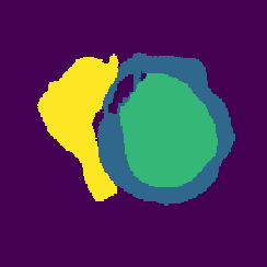
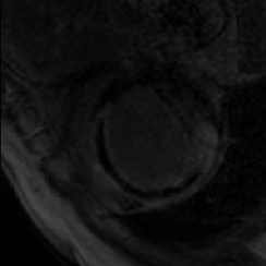
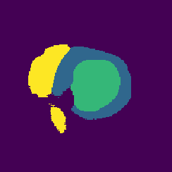
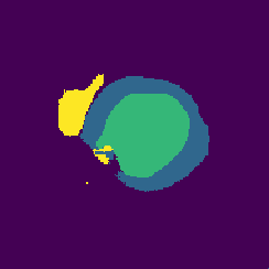
Figure 6: Segmentation output from MS-CMRSeg Dataset (bSSFP to LGE-MRI). From left to right: LGE-MRI, Ground truth, CFDNet[33], UDA-VAE[34], UDA-VAE++. For the segmentation, we use yellow, green, and dark green to represent RV, MYO, and LV, respectively.

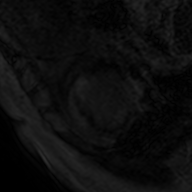
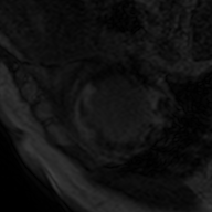
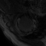
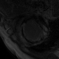
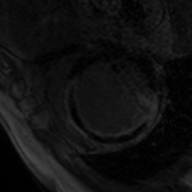
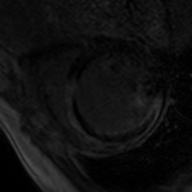
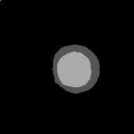
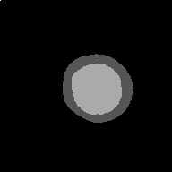
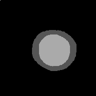
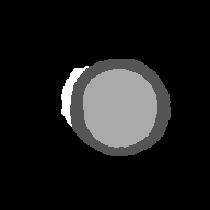
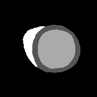
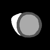
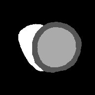
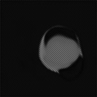
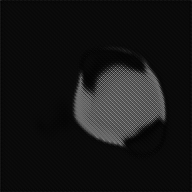
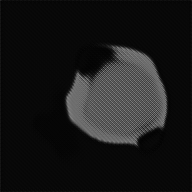
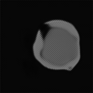
Figure 7: Reconstruction Images from MS-CMRSeg Dataset (LGE-MRI). From top to bottom row: LGE-MRI images, corresponding segmentation ground truth, UDA-VAE, UDA-VAE++.

4.1 Implementation Details

We use Adam optimizer [18] and Pytorch framework [26] to train our model for 30 epochs. The learning rate is initialized at 1e-4 and is reduced by 10 % after every epoch. The batch size is 12, which takes about 1 hour to converge on a single NVIDIA Tesla V100 GPU. The network weight follows Xavier initialization [8]. Neither gradient scaling nor gradient clipping is applied during training.

4.2 Datasets

We consider two benchmark datasets for model performance comparison, including Multi-Modality Whole Heart Segmentation (MM-WHS) Challenge dataset [41] and Multi-Sequence Cardiac MR Segmentation (MS-CMRSeg) Challenge dataset [40]

MM-WHS Dataset contains 20 labeled CT 3D images and 20 labeled MRI 3D images, which are unpaired. The original size of all images is 240$\times$220, which are cropped with a Region of Interest (ROI) of 192 × 192.

MS-CMRSeg Dataset contains 35 labeled bSSFP CMR 3D images and 45 labeled 3D LGE-MRI images, which are also not paired. Each image is cropped to a size of 192$\times$192.

Similar to [33, 34], we include the following three structures in MS-CMRSeg dataset for segmentation: the myocardial (MYO), the left ventriculus (LV), and the right ventriculus (RV). In MM-WHS Dataset, we include five structures: the myocardial (MYO), the left ventriculus (LV), the right ventriculus (RV), the left atrium blood cavity (LA), and the right atrium blood cavity (RA). For both datasets, We remove the LGE-MRI ground truth during bSSFP to LGE-MRI experiments, remove the bSSFP ground truth during LGE-MRI to bSSFP, and remove the MRI ground truth during CT to MRI experiments. The train-test split strategy is consistent with [5, 2, 33, 34]

4.3 Evaluation Metrics

We use three commonly used evaluation metrics for segmentation, including Dice coefficient (%) and Average Symmetric Surface Distance (ASSD) (mm). The Dice coefficient calculates the agreement between the predicted segmentation and ground truth segmentation by dividing the intersection area by the total pixels in both images. ASSD measures the segmentation accuracy at boundary-level using the Euclidean distance of the closest surface voxels between two segmentations [11]. All metrics are in the format of the mean. A higher Dice and a lower ASSD score indicate better segmentation performances.

4.4 Ablation Study

In this subsection, we investigate the contribution of our model components via an ablation study, using the Dice coefficient as the evaluation metric. Specifically, we gradually add individual components and see how the presence of that component will affect the model performances.

Table 2 shows the quantitative results of the ablation study. It is shown that most proposed modules will improve the Dice scores. For example, sequential reparameterization, adding Attention, Global, and Local MI estimation increases the Dice score for MYO, LV, and RV. Besides, prior info matching will slightly decrease RV but significantly increase MYO and LV, indicating overall performance improvement.

4.5 Qualitative Comparison

Fig. 6 shows the visual comparison for segmentation among different models, including CFDNet, UDA-VAE, and the proposed UDA-VAE++. It is shown that the proposed UDA-VAE++ leads to the best structure representation, the best edge preservation, and is the closest to the ground truth. In contrast, CFDNet and UDA-VAE have a significant segmentation error between MYO, RV, and the background.

Fig. 7 displays the visual comparison for reconstruction between different models. Here we only compare UDA-VAE++ with UDA-VAE since UDA-VAE is the only related work that considers image reconstruction. It is shown that the proposed UDA-VAE++ displays significantly better reconstruction than UDA-VAE. UDA-VAE++ has excellent edge preservation, shape representation, and class segmentation. In comparison, UDA-VAE has a significant amount of blurs and artifacts.

4.6 Quantitative Comparison

The quantitative comparison utilize several state-of-the-art models, including PnP-AdaNet [5], SIFA [2], UDA-VAE [34], and the proposed UDA-VAE++.

Table 3 shows the quantitative comparison for UDA with MS-CMRSeg Dataset (bSSFP to LGE-MRI). We can find that the proposed UDA-VAE++ has the best Dice and ASSD score in terms of MYO and LV segmentation. While SIFA has a slight advantage for RV segmentation, it underperforms our model for all other metrics in the table. Therefore, we can conclude that the proposed UDA-VAE++ has the best performance in this experiment.

Table 4 shows the quantitative comparison for UDA with MM-WHS Dataset (CT to MRI). We can observe that the proposed UDA-VAE++ has the best Dice and ASSD score in terms of MYO and LV segmentation. Despite SIFA’s success in Dice score at RV segmentation, it significantly underperforms our method for all other metrics. Overall, the proposed UDA-VAE++ has the best result in this comparison.

Table 5 shows the quantitative comparison for UDA with MS-CMRSeg Dataset (LGE-MRI to bSSFP). We can see that the proposed UDA-VAE++ has the best Dice and ASSD score in terms of all segmentations (MYO, LA, LV, RA, RV).

5 Conclusion

This paper introduces UDA-VAE++, an unsupervised domain adaptation framework for cardiac segmentation. Through mutual information estimation and maximization, we make the reconstruction and segmentation task mutually beneficial. Moreover, we introduce the sequential reparameterization design, allowing information flow between multi-scale latent space features. Extensive experiments demonstrate that our model achieved state-of-the-art performances on benchmark datasets. Our future work will integrate the proposed mutual information estimation block with self-supervised domain adaptation methods. We also aim to extend our framework to other medical image segmentation tasks (e.g., brain image segmentation).

6 Acknowledgement

We appreciate Dr. Fuping Wu and Zirui Wang’s kind help with mathematical deduction understanding and model workflow advice.

7 Supplementary Material

Proof of Eq.4:
Firstly, We follow the deduction from UDA-VAE[34].

$$\log p_{\theta_{S}}(x,y)$$ (14)

$$= \int q_{\phi_{S}}(z\mid x,y)\cdot$$

$$\log\left[\frac{q_{\phi_{S}}(z\mid x,y)}{p_{\theta_{S}}(z\mid x,y)}\cdot\frac{p_{\theta_{S}}(z)}{q_{\phi_{S}}(z\mid x,y)}\cdot p_{\theta_{S}}(x,y\mid z)\right]dz$$

$$= D_{KL}\left(q_{\phi_{S}}(z\mid x,y)\|p_{\theta_{S}}(z\mid x,y)\right)-$$

$$D_{KL}\left(q_{\phi_{S}}(z\mid x,y)\|p_{\theta_{S}}(z)\right)+$$

$$E_{q_{\phi_{S}}(z\mid x,y)}\log\left[p_{\theta_{S}}(x,y\mid z)\right]$$

Note that UDA-VAE[34] neglects the term $D_{KL}\left(q_{\phi_{S}}(z\mid x,y)\|p_{\theta_{S}}(z\mid x,y)\right)$ as it is greater than 0.
In comparison, we deduce a compact lower bound with the following term.

$$D_{KL}\left(q_{\phi_{S}}(z\mid x,y)\|p_{\theta_{S}}(z\mid x,y)\right)$$ (15)

$$=\int q_{\phi_{S}}(z\mid x,y)\log\frac{q_{\phi_{S}}(z\mid x,y)}{p_{\theta_{S}}(z\mid x,y)}dz$$

$$=\int\frac{q_{\phi_{S}}(x,y,z)}{q_{\phi_{S}}(x,y)}\log\frac{q_{\phi_{S}}(x,y,z)}{p_{\theta_{S}}(x,y,z)}\frac{p_{\theta_{S}}(x,y)}{q_{\phi_{S}}(x,y)}dz$$

$$=\frac{1}{q_{\phi_{S}}(x,y)}[\int q_{\phi_{S}}(x,y,z)\log\frac{q_{\phi_{S}}(x,y,z)}{p_{\theta_{S}}(x,y,z)}$$

$$+q_{\phi_{S}}(x,y,z)\log\frac{p_{\theta_{S}}(x,y)}{q_{\phi_{S}}(x,y)}dz]$$

$$=\frac{1}{q_{\phi_{S}}(x,y)}\int q_{\phi_{S}}(x,y,z)\log\frac{q_{\phi_{S}}(x,y,z)}{p_{\theta_{S}}(x,y,z)}dz$$

$$+\log\frac{p_{\theta_{S}}(x,y)}{q_{\phi_{S}}(x,y)}$$

$$=\frac{1}{q_{\phi_{S}}(x,y)}D_{KL}(q_{\phi_{S}}(x,y,z)\|p_{\theta_{S}}(x,y,z))$$

$$+\log\frac{p_{\theta_{S}}(x,y)}{q_{\phi_{S}}(x,y)}$$

$$\geq D_{KL}(q_{\phi_{S}}(x,y,z)\|p_{\theta_{S}}(x,y,z))+\log\frac{p_{\theta_{S}}(x,y)}{q_{\phi_{S}}(x,y)}$$

Consider the reconstruction error[1]:

$$\mathcal{R}= \mathbb{E}_{(x,y,z)\sim}q_{\phi_{S}}(x,y,z)\log\frac{q_{\phi_{S}}(x,y,z)}{p_{\theta_{S}}(x,y,z)}-$$ (16)

$$\mathbb{E}_{(x,y,z)\sim q_{\phi_{S}}(x,y,z)}\log q_{\phi_{S}}(x,y,z)+\mathbb{E}_{z\sim q_{\phi_{S}}(z)}\log p_{\theta_{S}}(z)$$

The second term is the joint entropy $H_{q}(x,y,z)$.
The third term can be written as:

$$\mathbb{E}_{z\sim q_{\phi_{S}}(z)}\log p_{\theta_{S}}(z)=-D_{KL}(q_{\phi_{S}(z)}\|p_{\theta_{S}})-H_{q_{\phi_{S}}}(z)$$ (17)

With

$$H_{q_{\phi_{S}(z)}}(x,y,z)-H_{q_{\phi_{S}}}(z)=H_{q_{\phi_{S}}}(z)-I_{q_{\phi_{S}}}(x,y,z)$$ (18)

where $I$ is mutual information.
The reconstruction error can be written as:

$$\mathcal{R}\leq D_{KL}(q_{\phi_{S}(x,y,z)}\|p_{\theta_{S}(x,y,z)})-I_{q_{\phi_{S}}}(x,y,z)+H_{q_{\phi_{S}}}(z)$$ (19)

which is compact when $q_{\phi_{S}(z)}$ matches the prior distribution $p_{\theta_{S}}(z)$.

$$D_{KL}(q_{\phi_{S}(x,y,z)}\|p_{\theta_{S}(x,y,z)})\geq\mathcal{R}+I_{q_{\phi_{S}}}(x,y,z)-H_{q_{\phi_{S}}}(z)$$ (20)

Thus, we obtain the bound,

$$D_{KL}\left(q_{\phi_{S}}(z\mid x,y)\|p_{\theta_{S}}(z\mid x,y)\right)$$ (21)

$$\geq D_{KL}(q_{\phi_{S}}(x,y,z)\|p_{\theta_{S}}(x,y,z))+\log\frac{p_{\theta_{S}}(x,y)}{q_{\phi_{S}}(x,y)}$$

$$\geq\mathcal{R}+I_{q_{\phi_{S}}}(x,y,z)-H_{q_{\phi_{S}}}(z)+\log\frac{p_{\theta_{S}}(x,y)}{q_{\phi_{S}}(x,y)}$$

From, Eq.14 and Eq.21,

$$\log p_{\theta_{S}}(x,y)$$ (22)

$$\geq {\color[rgb]{1,0,0}(\mathcal{R}+I_{q_{\phi_{S}}}(x,y,z)-H_{q_{\phi_{S}}}(z)+\log\frac{p_{\theta_{S}}(x,y)}{q_{\phi_{S}}(x,y)})}-$$

$$D_{KL}\left(q_{\phi_{S}}(z\mid x)\|p_{\theta_{S}}(z)\right)+E_{q_{\phi_{S}}(z\mid x)}\log p_{\theta_{S}}(x,y\mid z)$$

$$= {\color[rgb]{1,0,0}(\mathcal{R}+I_{q_{\phi_{S}}}(x,y,z)-H_{q_{\phi_{S}}}(z)+\log\frac{p_{\theta_{S}}(x,y)}{q_{\phi_{S}}(x,y)})}-$$

$$D_{KL}\left(q_{\phi_{S}}(z\mid x)\|p_{\theta_{S}}(z)\right)+E_{q_{\phi_{S}}(z\mid x)}\log p_{\theta_{S}}(x\mid y,z)$$

$$+E_{q_{\phi_{S}}(z\mid x)}\log p_{\theta_{S}}(y\mid z)$$

where $R$, $\log\frac{p_{\theta_{S}}(x,y)}{q_{\phi_{S}}(x,y)}$ and $H_{q_{\phi_{S}}}(z)$ are constant. The equation holds, as $p_{\theta_{S}}(x,y\mid z)=p_{\theta_{S}}(y\mid z)\cdot p_{\theta_{S}}(x\mid y,z)$. Meanwhile, $y_{S}$ and $z_{s}$ are conditionally independent on $x_{S}$ for distribution $q_{\phi_{S}}$, so that $q_{\phi_{S}}(z\mid x,y)=q_{\phi_{S}}(z\mid x)$.
Finally, We get the compact lower bound (plus red terms) than UDA-VAE .
The UDA-VAE++ maximizes the mutual information of $I_{q_{\phi_{S}}}(x,y,z)$.
Proved.

References

- [1] Mohamed Ishmael Belghazi, Aristide Baratin, Sai Rajeshwar, Sherjil Ozair, Yoshua Bengio, Aaron Courville, and Devon Hjelm. Mutual information neural estimation. In International conference on machine learning, pages 531–540. PMLR, 2018.
- [2] Cheng Chen, Qi Dou, Hao Chen, Jing Qin, and Pheng Ann Heng. Unsupervised bidirectional cross-modality adaptation via deeply synergistic image and feature alignment for medical image segmentation. IEEE transactions on medical imaging, 39(7):2494–2505, 2020.
- [3] Qingchao Chen and Yang Liu. Structure-aware feature fusion for unsupervised domain adaptation. In Proceedings of the AAAI Conference on Artificial Intelligence, volume 34, pages 10567–10574, 2020.
- [4] Monroe D Donsker and SR Srinivasa Varadhan. Asymptotic evaluation of certain markov process expectations for large time, i. Communications on Pure and Applied Mathematics, 28(1):1–47, 1975.
- [5] Qi Dou, Cheng Ouyang, Cheng Chen, Hao Chen, Ben Glocker, Xiahai Zhuang, and Pheng-Ann Heng. Pnp-adanet: Plug-and-play adversarial domain adaptation network at unpaired cross-modality cardiac segmentation. IEEE Access, 7:99065–99076, 2019.
- [6] Qi Dou, Cheng Ouyang, Cheng Chen, Hao Chen, and Pheng-Ann Heng. Unsupervised cross-modality domain adaptation of convnets for biomedical image segmentations with adversarial loss. arXiv preprint arXiv:1804.10916, 2018.
- [7] Qi Dou, Lequan Yu, Hao Chen, Yueming Jin, Xin Yang, Jing Qin, and Pheng-Ann Heng. 3d deeply supervised network for automated segmentation of volumetric medical images. Medical image analysis, 41:40–54, 2017.
- [8] Xavier Glorot and Yoshua Bengio. Understanding the difficulty of training deep feedforward neural networks. In Proceedings of the thirteenth international conference on artificial intelligence and statistics, pages 249–256. JMLR Workshop and Conference Proceedings, 2010.
- [9] Ian Goodfellow, Jean Pouget-Abadie, Mehdi Mirza, Bing Xu, David Warde-Farley, Sherjil Ozair, Aaron Courville, and Yoshua Bengio. Generative adversarial nets. Advances in neural information processing systems, 27, 2014.
- [10] Mingxuan Gu, Sulaiman Vesal, Ronak Kosti, and Andreas Maier. Few-shot unsupervised domain adaptation for multi-modal cardiac image segmentation. arXiv preprint arXiv:2201.12386, 2022.
- [11] Tobias Heimann, Bram Van Ginneken, Martin A Styner, Yulia Arzhaeva, Volker Aurich, Christian Bauer, Andreas Beck, Christoph Becker, Reinhard Beichel, György Bekes, et al. Comparison and evaluation of methods for liver segmentation from ct datasets. IEEE transactions on medical imaging, 28(8):1251–1265, 2009.
- [12] Martin Heusel, Hubert Ramsauer, Thomas Unterthiner, Bernhard Nessler, and Sepp Hochreiter. Gans trained by a two time-scale update rule converge to a local nash equilibrium. Advances in neural information processing systems, 30, 2017.
- [13] R Devon Hjelm, Alex Fedorov, Samuel Lavoie-Marchildon, Karan Grewal, Phil Bachman, Adam Trischler, and Yoshua Bengio. Learning deep representations by mutual information estimation and maximization. arXiv preprint arXiv:1808.06670, 2018.
- [14] Phillip Isola, Jun-Yan Zhu, Tinghui Zhou, and Alexei A Efros. Image-to-image translation with conditional adversarial networks. In Proceedings of the IEEE conference on computer vision and pattern recognition, pages 1125–1134, 2017.
- [15] Vicky Kalogeiton, Vittorio Ferrari, and Cordelia Schmid. Analysing domain shift factors between videos and images for object detection. IEEE transactions on pattern analysis and machine intelligence, 38(11):2327–2334, 2016.
- [16] Tero Karras, Samuli Laine, and Timo Aila. A style-based generator architecture for generative adversarial networks. In Proceedings of the IEEE/CVF conference on computer vision and pattern recognition, pages 4401–4410, 2019.
- [17] Tero Karras, Samuli Laine, Miika Aittala, Janne Hellsten, Jaakko Lehtinen, and Timo Aila. Analyzing and improving the image quality of stylegan. In Proceedings of the IEEE/CVF conference on computer vision and pattern recognition, pages 8110–8119, 2020.
- [18] Diederik P Kingma and Jimmy Ba. Adam: A method for stochastic optimization. arXiv preprint arXiv:1412.6980, 2014.
- [19] Diederik P Kingma and Max Welling. Auto-encoding variational bayes. arXiv preprint arXiv:1312.6114, 2013.
- [20] Diederik P Kingma and Max Welling. Auto-encoding variational bayes. arXiv preprint arXiv:1312.6114, 2013.
- [21] Diederik P Kingma and Max Welling. An introduction to variational autoencoders. arXiv preprint arXiv:1906.02691, 2019.
- [22] Yueguo Liu and Xiuquan Du. Duda: Deep unsupervised domain adaptation learning for multi-sequence cardiac mr image segmentation. In Chinese Conference on Pattern Recognition and Computer Vision (PRCV), pages 503–515. Springer, 2020.
- [23] Yun Liu, Krishna Gadepalli, Mohammad Norouzi, George E Dahl, Timo Kohlberger, Aleksey Boyko, Subhashini Venugopalan, Aleksei Timofeev, Philip Q Nelson, Greg S Corrado, et al. Detecting cancer metastases on gigapixel pathology images. arXiv preprint arXiv:1703.02442, 2017.
- [24] Alireza Makhzani, Jonathon Shlens, Navdeep Jaitly, Ian Goodfellow, and Brendan Frey. Adversarial autoencoders. arXiv preprint arXiv:1511.05644, 2015.
- [25] Cheng Ouyang, Konstantinos Kamnitsas, Carlo Biffi, Jinming Duan, and Daniel Rueckert. Data efficient unsupervised domain adaptation for cross-modality image segmentation. In International Conference on Medical Image Computing and Computer-Assisted Intervention, pages 669–677. Springer, 2019.
- [26] Adam Paszke, Sam Gross, Francisco Massa, Adam Lerer, James Bradbury, Gregory Chanan, Trevor Killeen, Zeming Lin, Natalia Gimelshein, Luca Antiga, et al. Pytorch: An imperative style, high-performance deep learning library. Advances in neural information processing systems, 32, 2019.
- [27] Andrew J. Peacock and Anton Vonk Noordegraaf. Cardiac magnetic resonance imaging in pulmonary arterial hypertension. European Respiratory Review, 22(130):526–534, 2013.
- [28] Sanjay Purushotham, Wilka Carvalho, Tanachat Nilanon, and Yan Liu. Variational recurrent adversarial deep domain adaptation. 2016.
- [29] Olaf Ronneberger, Philipp Fischer, and Thomas Brox. U-net: Convolutional networks for biomedical image segmentation. In International Conference on Medical image computing and computer-assisted intervention, pages 234–241. Springer, 2015.
- [30] Gerard Snaauw, Michele Sasdelli, Gabriel Maicas, Stephan Lau, Johan Verjans, Mark Jenkinson, and Gustavo Carneiro. Mutual information neural estimation for unsupervised multi-modal registration of brain images. arXiv preprint arXiv:2201.10305, 2022.
- [31] Juiwen Ting, Kumaradevan Punithakumar, and Nilanjan Ray. Multiview 3-d echocardiography image fusion with mutual information neural estimation. In 2020 IEEE International Conference on Bioinformatics and Biomedicine (BIBM), pages 765–771. IEEE, 2020.
- [32] Tatiana Tommasi, Martina Lanzi, Paolo Russo, and Barbara Caputo. Learning the roots of visual domain shift. In European Conference on Computer Vision, pages 475–482. Springer, 2016.
- [33] Fuping Wu and Xiahai Zhuang. Cf distance: A new domain discrepancy metric and application to explicit domain adaptation for cross-modality cardiac image segmentation. IEEE Transactions on Medical Imaging, 39(12):4274–4285, 2020.
- [34] Fuping Wu and Xiahai Zhuang. Unsupervised domain adaptation with variational approximation for cardiac segmentation. IEEE Transactions on Medical Imaging, 40(12):3555–3567, 2021.
- [35] Ke Yan, Youbao Tang, Yifan Peng, Veit Sandfort, Mohammadhadi Bagheri, Zhiyong Lu, and Ronald M Summers. Mulan: multitask universal lesion analysis network for joint lesion detection, tagging, and segmentation. In International Conference on Medical Image Computing and Computer-Assisted Intervention, pages 194–202. Springer, 2019.
- [36] Wenjun Yan, Yuanyuan Wang, Shengjia Gu, Lu Huang, Fuhua Yan, Liming Xia, and Qian Tao. The domain shift problem of medical image segmentation and vendor-adaptation by unet-gan. In International Conference on Medical Image Computing and Computer-Assisted Intervention, pages 623–631. Springer, 2019.
- [37] Zizhao Zhang, Lin Yang, and Yefeng Zheng. Translating and segmenting multimodal medical volumes with cycle-and shape-consistency generative adversarial network. In Proceedings of the IEEE conference on computer vision and pattern Recognition, pages 9242–9251, 2018.
- [38] Jun-Yan Zhu, Taesung Park, Phillip Isola, and Alexei A Efros. Unpaired image-to-image translation using cycle-consistent adversarial networks. In Proceedings of the IEEE international conference on computer vision, pages 2223–2232, 2017.
- [39] Xiahai Zhuang. Challenges and methodologies of fully automatic whole heart segmentation: a review. Journal of healthcare engineering, 4(3):371–407, 2013.
- [40] Xiahai Zhuang. Multivariate mixture model for myocardial segmentation combining multi-source images. IEEE transactions on pattern analysis and machine intelligence, 41(12):2933–2946, 2018.
- [41] Xiahai Zhuang and Juan Shen. Multi-scale patch and multi-modality atlases for whole heart segmentation of mri. Medical image analysis, 31:77–87, 2016.