Deterministic Distributed algorithms and Descriptive Combinatorics on $\Delta$-regular trees

Abstract

We study complexity classes of local problems on regular trees from the perspective of distributed local algorithms and descriptive combinatorics. We show that, surprisingly, some deterministic local complexity classes from the hierarchy of distributed computing exactly coincide with well studied classes of problems in descriptive combinatorics. Namely, we show that a local problem admits a continuous solution if and only if it admits a local algorithm with local complexity $O(\log^{*}n)$, and a Baire measurable solution if and only if it admits a local algorithm with local complexity $O(\log n)$.

1 Introduction

This work is a part of a research program which investigates the connections between the area of distributed computing and descriptive combinatorics. The first connections of this sort have been formalized in the seminal paper of Bernshteyn [Ber20a] (see also [Ele18]). Since then, many exciting results confirmed the importance of this approach [CGA⁺16, GR21b, GR21a, BCG⁺21c, BCG⁺21b, Ber20b], some of which also build a connection to the area of random processes. Combined with the work in each field such as [Lin92, HSW17, Mar16, GJKS18, GJKS, BFH⁺16, BHK⁺17], a rich picture of a common theory of locality starts to emerge.

The definition of the $\mathsf{LOCAL}$ model of distributed computing by Linial [Lin92] was motivated by the desire to understand distributed algorithms in huge networks. Informally, we have the following setup. Let $G$ be a finite graph, where each vertex is imagined to be a computer, which knows the size of the graph $n$, and perhaps some other parameters like the maximum degree $\Delta$. Every computer runs the same algorithm. In order to break the symmetries, each computer possesses some unique information, such as a natural number in the case of deterministic algorithms or a random bit string in the case of randomized ones. In one round, each vertex can exchange any message with its neighbors and can perform an arbitrary computation. The goal is to find a solution to a given graph theoretic problem (more precisely, LCL, see below) in as few communication rounds as possible. The theory of distributed algorithms and the $\mathsf{LOCAL}$ model is extremely rich and deep, see, e.g., [BEPS16, CKP19, CP19, GKM17, KMW16, RG20].

Descriptive or measurable combinatorics is an emerging field on the border of combinatorics, logic, group theory, and ergodic theory. The highlights of the field include the recent results on the circle squaring problem of Tarski [GMP17, MU17, MNP22], or on the Banach-Tarski paradox [DF92, MU16], see also [Lac90, MU17, GMP17, DF92, MU16, Gab00, KST99, Mar16, CM17, CJM⁺20, CGM⁺17, Ber20a], and [KM20, Pik21] for surveys. The usual setup in descriptive combinatorics is that we have a graph with uncountably many connected components, each being a countable graph of bounded degree, and we want to find a solution to a given graph theoretic problem with some additional regularity (measurability) properties. We refer the reader less familiar with distributed computing (resp. descriptive combinatorics) to Section 2.2 (the first part of Section 2.4) for the definitions of some of the most relevant concepts.

The common link between the two areas is played by so-called locally checkable labeling (LCL) problems on graphs, which is a class of problems, where the correctness of a solution can be checked locally, that is, in a fixed sized neighborhood of vertices. Examples include classical problems from combinatorics such as proper vertex coloring, proper edge coloring, perfect matching, and finding a maximal independent set.

One can order the collection of LCLs to complexity classes, based on the asymptotic number of turns required to solve them in the $\mathsf{LOCAL}$ model, and based on the measurability properties of the solution in descriptive combinatorics. Hence the natural question of comparing these classes arises. In the insightful papers [Ber20a, Ber21], Bernshteyn showed the equality of some of these classes: roughly speaking, fast local algorithms solving LCLs yield measurable solutions, and conversely, in the context of Cayley graphs of countable groups continuous solutions give back fast local algorithms.

In this paper, we focus on LCLs on (finite and infinite) $\Delta$-regular trees (see Section 2). The motivation for studying regular trees stems from different sources:

• The case of trees is one of the highlights of the theory of the LOCAL model. For example, several lower bounds in distributed computing are proven for regular trees [BBE⁺20, BBH⁺19, BBKO21, BBKO22, BBO20, BFH⁺16, Bra19, BO20, CHL⁺20, GHS14]; a classification of all the potential complexity classes of LCLs is also known in this context (see Theorem 2.6).

• In many of the aforementioned results of descriptive combinatorics, including the Banach-Tarski paradox, graphs where each component is an infinite $\Delta$-regular tree appear naturally. Moreover, such trees are also studied in the area of ergodic theory [Bow10b, Bow10a] and random processes [BGH19, BSV15, LN11].

• Comparing the techniques coming from these perspectives in this simple setting reveals already deep connections.

Broadly speaking, our main results are the following. First, we extend the correspondence of Bernshteyn [Ber21] to regular trees, that is, we show that the class of LCLs that admit a continuous solution and a solution by a fast deterministic algorithm are the same. Second, we show that there is an exact equality “high up” in the hierarchy, namely, the class of LCLs on regular trees that admit a local algorithm of local deterministic complexity $O(\log n)$ coincides with the class of LCLs that admit so called Baire measurable solution, see Fig. 1.

Before we discuss our results in more details, we remark that [BCG⁺21c, BCG⁺21a] and this paper extend the conference paper [BCG⁺21b]. In addition to the two perspectives studied here, we study LCLs from the perspective of random processes in [BCG⁺21a]. We refer the reader to [BCG⁺21a] or [BCG⁺21b] for more details of the “big picture.”

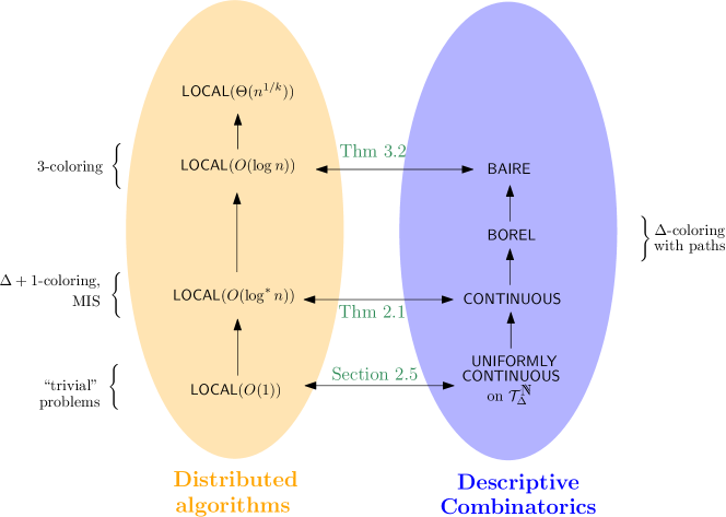
Figure 1: Complexity classes on $\Delta$-regular trees considered in the areas of distributed computing and descriptive combinatorics. The left part shows deterministic complexity classes of distributed computing. The black arrows with two endpoints represent equalities between the complexity classes. The black arrows with just one endpoint stand for proper inclusions between the classes. We highlight two phenomena. First, we have $\mathsf{LOCAL}(O(\log^{*}n))=\mathsf{CONTINUOUS}$, that is, there is a natural class of basic symmetry breaking problems in both areas. Second, we have $\mathsf{LOCAL}(O(\log n))=\mathsf{BAIRE}$, that is, the most powerful class in descriptive combinatorics exactly matches the power of finite local construction with local complexity $O(\log n)$.

The results

$\mathsf{LOCAL}(f(n))$ denotes the class of LCLs of deterministic local complexity $f(n)$ (see Definition 2.5, and the discussion thereafter). The complexity classes of local problems that always admit a solution with the respective regularity properties that we consider in the paper are $\mathsf{CONTINUOUS},\mathsf{BOREL},\mathsf{BAIRE}$; see Section 2.4.

Once the complexity classes are defined, we can state the connections in a compact form, e.g., $\mathsf{LOCAL}(O(\log^{*}n))=\mathsf{CONTINUOUS}$. Indeed, as mentioned above, this equality was proven in [Ber21] for Cayley graphs of countable groups. Our first result extends this result to the context of $\Delta$-regular trees. We note that [Ber21] includes the case of the $\Delta$-regular tree endowed with a proper $\Delta$-edge coloring. However, as the proper $\Delta$-edge coloring problem can be solved neither by a continuous nor by a Borel function [Mar16], we see that these models are different. Importantly, the automorphism group of the infinite $\Delta$-regular tree without edge coloring is significantly bigger than the one that preserves the coloring structure.

Theorem 1.1.

We have

$$\mathsf{LOCAL}(O(\log^{*}n))=\mathsf{CONTINUOUS}$$

for LCLs on $\Delta$-regular trees.

The direction from left to right follows already from [Ber20a], see also [Ele18]. On a high level, it uses the speedup result of [CKP19] that implies that every LCL of complexity $O(\log^{*}n)$ can be solved by first solving the $k$-distance coloring problem on the underlying graph, for some $k\in\mathbb{N}$, and then applying a constant local rule. These operations can be performed using continuous functions by [KST99], see also [Ber21, Section 2]. The other direction should be interpreted as an equivalence of several models for continuous solutions, see Section 2 and Theorem 3.1. Most notably it captures the $\{0,1\}$-model that has been studied extensively in the context of countable groups [GJS09, STD16, GJKS18, Ber21]. Intuitively, a given LCL can be solved in the $\{0,1\}$-model if there is a map (local rule) $\mathcal{A}$ with a subset of $\{0,1\}$-labeled neighborhoods of vertices of the infinite $\Delta$-regular tree $T_{\Delta}$ as a domain that assigns to each neighborhood from the domain some labeling such that the following holds. Whenever we are given a $\{0,1\}$-labeling of $T_{\Delta}$ that breaks all the symmetries of $T_{\Delta}$, then we can run $\mathcal{A}$ at every vertex and the output given by $\mathcal{A}$ is a solution to the given LCL. Here by “running $\mathcal{A}$” we mean that each vertex explores its neighborhood until it encounters a $\{0,1\}$-labeled neighborhood that is in the domain of $\mathcal{A}$; the output at the vertex is then the output of $\mathcal{A}$ applied on this neighborhood of the vertex. The overall strategy to show that LCLs solvable in this model have local deterministic complexity exactly $O(\log^{*}n)$ follows [Ber21], in particular we use Bernshteyn’s continuous version of the Lovász Local Lemma, and the framework from [GJKS18]. However, as our underlying graph is not induced by a group action some additional non-trivial arguments are needed. It is an interesting open problem to study the $\{0,1\}$-labeling model on other classes of (structured) graphs.

Next we describe the main result of the paper. Recently, Bernshteyn proved [Ber] that all LCLs on $\Delta$-regular trees that are in the complexity class $\mathsf{BAIRE}$, i.e., that admit Baire measurable solutions, have to satisfy a simple combinatorial condition which we call being $\ell$-full (we defer the formal definition of $\ell$-fullness to Section 4). On the other hand, all $\ell$-full problems allow a $\mathsf{BAIRE}$ solution [Ber]. This implies a complete combinatorial characterization of the class $\mathsf{BAIRE}$. We include a proof of his result for the sake of completeness. Our proof is based on a hierarchical decomposition called toast. Toasts recently became a prominent tool in combinatorial constructions on the descriptive side, see e.g. [MU17, MNP22, Bow10a]. The key observation is that one can construct toasts in a Baire measurable manner (Proposition 2.27) and from this one can solve the LCL assuming it is $\ell$-full. Informally speaking, in the context of vertex labeling problems, a problem is $\ell$-full if we can choose a subset $S$ of the labels with the following property. Whenever we label two endpoints of a path of at least $\ell$ vertices with two labels from $S$, we can extend the labeling with labels from $S$ to the whole path such that the overall labeling is valid. For example, proper $3$-coloring is $3$-full with $S=\{1,2,3\}$ because for any path of three vertices such that its both endpoints are colored arbitrarily, we can color the middle vertex so that the overall coloring is proper. On the other hand, proper $2$-coloring is not $\ell$-full for any $\ell$.

We complement this result as follows. First, we prove that any $\ell$-full problem has local complexity $O(\log n)$. Interestingly, this implies that all complexity classes considered in [BCG⁺21a], most notably LCLs that admit factor of iid solution, are contained in $\mathsf{LOCAL}(O(\log n))$. In particular, this implies that the existence of any uniform algorithm implies a local distributed algorithm for the same problem of local complexity $O(\log n)$, see [BCG⁺21a] for details. We obtain this result via the well-known rake-and-compress decomposition [MR89].

On the other hand, we prove that any problem in the class $\mathsf{LOCAL}(O(\log n))$ satisfies the $\ell$-full condition. The proof combines a machinery developed by Chang and Pettie [CP19] with additional ideas. In this proof we construct recursively a sequence of sets of rooted, layered, and partially labeled trees, where the partial labeling is computed by simulating any given $O(\log n)$-round distributed algorithm, and then the set $S$ meeting the $\ell$-full condition is constructed by considering all possible extensions of the partial labeling to complete a correct labeling of these trees. In summary, we have the following rather surprising equality.

Theorem 1.2.

We have

$$\mathsf{LOCAL}(O(\log n))=\mathsf{BAIRE}$$

for LCLs on $\Delta$-regular trees.

The combinatorial characterization of the local complexity class $\mathsf{LOCAL}(O(\log n))$ on $\Delta$-regular trees is interesting from the perspective of distributed computing alone. This result can be seen as a part of a large research program aiming at the combinatorial classification of possible local complexities on various graph classes [BBOS20, BFH⁺16, CKP19, CP19, Cha20, CSS20, BBO⁺21, BBE⁺20, BHK⁺18]. That is, we wish not only to understand the possible complexity classes (see the left part of Fig. 1 for the possible local complexity classes on regular trees), but also to find combinatorial characterizations of problems in those classes that allow us to efficiently decide for a given problem which class it belongs to. Unfortunately, even for grids with input labels, it is undecidable whether a given local problem can be solved in $O(1)$ rounds [NS95, BHK⁺17], since local problems on grids can be used to simulate a Turing machine. This undecidability result does not apply to paths and trees, hence for these graph classes it is still hopeful that we can find simple and useful characterizations for different classes of distributed problems.

The paper is organized as follows. In Section 2, we recall all the notation, definitions, and standard results. In Section 3, we demonstrate the equality between the classes $\mathsf{LOCAL}(O(\log^{*}n))$ and $\mathsf{CONTINUOUS}$. In Section 4, we demonstrate the equality between the classes $\mathsf{LOCAL}(O(\log n))$ and $\mathsf{BAIRE}$.

2 Preliminaries

In this section, we explain the setup we work with, the main definitions, techniques and results. The class of graphs that we consider in this work are either infinite $\Delta$-regular trees, or their finite analogues that we define formally in Section 2.1. We implicitly assume that $\Delta>2$. The case $\Delta=2$, that is, studying paths, behaves differently and is easier to understand, see [GR21a]. Unless stated otherwise, we do not consider any additional structure on the graphs.

If $G$ is a graph, then we use $V(G)$ for its vertex set and $E(G)$ for the set of edges. We write $B_{G}(v,t)$ for the $t$-neighborhood of a vertex $v\in V(G)$. We denote as $N_{G}(A)$ the set of vertices in $G$ that are connected by an edge with some element from $A\subseteq V(G)$. The graph distance $dist_{G}$ is defined in the standard way. For $L\in\mathbb{N}$, we define the $L$-power graph of $G$ as the graph on the same vertex set where $v,w\in V(G)$ form an edge if and only if $0<dist_{G}(v,w)\leq L$. If we talk about acyclic graphs we use $T$ instead of $G$. To emphasize the difference between Borel graphs and discrete (at most countable) graphs, we use $\mathcal{G}$ and $\mathcal{T}$ in the former case. Vertices of discrete graphs are denoted as $v,w,\dots$ and of Borel graphs as $x,y,z,\alpha,\dots$. We write $T_{\Delta}$ for the $\Delta$-regular tree and $\mathfrak{r}$ for a fixed vertex of $T_{\Delta}$ that we call the root of $T_{\Delta}$. As $T_{\Delta}$ is the main object of our study, we omit the subscript in the notation above whenever we talk about $T_{\Delta}$ (that is, in the case of $B(\cdot,\cdot)$ and $dist$). Similarly, we use $v\in T_{\Delta}$ instead of $v\in V(T_{\Delta})$. Recall also that for $k\in\mathbb{N}$ and $v\in T_{\Delta}$, we have $|B(v,k)|=1+\Delta\sum_{i=0}^{k-1}(\Delta-1)^{i}$, we mostly use the upper bound $2\Delta^{k}$ which holds for every $k\in\mathbb{N}$.

For $k\in\mathbb{N}$ define the $k$th power of the graph $G$ to be the graph with vertex set $V(G)$, where two vertices are adjacent, if their distance is at most $k$. A $k$-distance coloring of $G$ is a coloring of the $k$th power of $G$, or equivalently, a coloring of $G$ where vertices of distance at most $k$ have different colors.

2.1 Local Problems on $\Delta$-regular trees

The problems we study in this work are locally checkable labeling (LCL) problems, which, roughly speaking, are problems that can be described via local constraints that have to be satisfied in a neighborhood of each vertex. In the context of distributed algorithms, these problems were introduced in the seminal work by Naor and Stockmeyer [NS95], and have been studied extensively since. In the modern formulation introduced in [Bra19], instead of labeling vertices or edges, LCL problems are described by labeling half-edges, i.e., pairs of a vertex and an adjacent edge. This formulation is very general in that it not only captures vertex and edge labeling problems, but also others such as orientation problems, or combinations of all of these types. Before we can provide this general definition of an LCL, we need to introduce some definitions. We start by formalizing the notion of a half-edge.

Definition 2.1 (Half-edge).

A half-edge is a pair $(v,e)$ where $v$ is a vertex, and $e$ an edge adjacent to $v$. We say that a half-edge $(v,e)$ is adjacent to a vertex $w$ if $w=v$. Equivalently, we say that $w$ is contained in $(v,e)$ if $(v,e)$ is adjacent to $w$. We say that $(v,e)$ belongs to an edge $e^{\prime}$ if $e^{\prime}=e$. We denote the set of all half-edges of a graph $G$ by $H(G)$. A half-edge labeling is a function $c\colon H(G)\to\Sigma$ that assigns to each half-edge an element from some label set $\Sigma$.

In order to speak about finite $\Delta$-regular trees, we need to consider a slightly modified definition of a graph. We imagine each vertex to be contained in $\Delta$-many half-edges. However, not every half-edge belongs to an actual edge of the graph. That is half-edges are pairs $(v,e)$, but $e$ is formally not a pair of vertices. Sometimes we refer to these half-edges as virtual half-edges. We include a formal definition to avoid confusions. See also Fig. 2.

Definition 2.2 ($\Delta$-regular trees).

A tree $T$, finite or infinite, is a $\Delta$-regular tree if one of the following holds. Either $T$ is infinite and $T=T_{\Delta}$ (where $T_{\Delta}$ is the unique infinite $\Delta$-regular tree), or, $T$ is a finite tree of maximum degree $\Delta$ and each vertex $v\in T$ of degree $d\leq\Delta$ is contained in $(\Delta-d)$-many virtual half-edges.

Formally, we can view $T$ as a triplet $(V(T),E(T),H(T))$, where $(V(T),E(T))$ is a tree of maximum degree $\Delta$ and $H(T)$ consists of real half-edges, that is pairs $(v,e)$, where $v\in V(T)$, $e\in E(T)$ and $e$ is adjacent to $v$, together with some virtual edges, in the case when $T$ is finite, such that each vertex $v\in V(T)$ is contained in exactly $\Delta$-many half-edges (real or virtual).

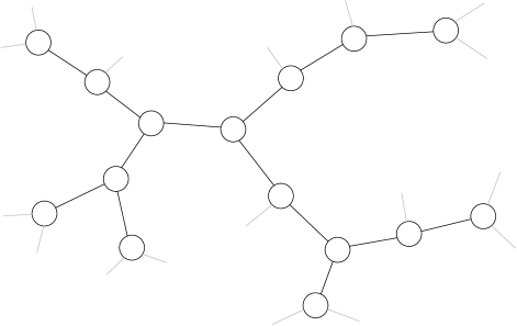
Figure 2: A $3$-regular tree on 15 vertices. Every vertex has $3$ half-edges but not all half-edges lead to a different vertex.

As we are considering trees in this work, each LCL problem can be described in a specific form that provides two lists, one describing all label combinations that are allowed on the half-edges adjacent to a vertex, and the other describing all label combinations that are allowed on the two half-edges belonging to an edge. We arrive at the following definition for LCLs on $\Delta$-regular trees.

Definition 2.3 (LCLs on $\Delta$-regular trees).

A locally checkable labeling problem, or LCL for short, is a triple $\Pi=(\Sigma,\mathcal{V},\mathcal{E})$, where $\Sigma$ is a finite set of labels, $\mathcal{V}$ is a subset of unordered cardinality-$\Delta$ multisets of labels from $\Sigma$, and $\mathcal{E}$ is a subset of unordered cardinality-$2$ multisets of labels from $\Sigma$.

We call $\mathcal{V}$ and $\mathcal{E}$ the vertex constraint and edge constraint of $\Pi$, respectively. Moreover, we call each multiset contained in $\mathcal{V}$ a vertex configuration of $\Pi$, and each multiset contained in $\mathcal{E}$ an edge configuration of $\Pi$.

Let $T$ be a $\Delta$-regular tree and $c:H(T)\to\Sigma$ a half-edge labeling of $T$ with labels from $\Sigma$. We say that $c$ is a $\Pi$-coloring, or, equivalently, a correct solution of $\Pi$, if, for each vertex $v$ of $T$, the multiset of labels assigned to the half-edges adjacent to $v$ is contained in $\mathcal{V}$, and, for each edge $e$ of $T$, the cardinality-$2$ multiset of labels assigned to the half-edges belonging to $e$ is an element of $\mathcal{E}$.

An equivalent way to define our setting would be to consider $\Delta$-regular trees as commonly defined, that is, there are vertices of degree $\Delta$ and vertices of degree $1$, i.e., leaves. In the corresponding definition of LCL one would consider leaves as unconstrained w.r.t. the vertex constraint, i.e., in the above definition of a correct solution the condition “for each vertex $v$” is replaced by “for each non-leaf vertex $v$”. To see the equivalence, consider our definition of a $\Delta$-regular tree and append a leaf to the “other side” of each virtual edge.

Equivalently, we could also allow arbitrary trees of maximum degree $\Delta$ as input graphs, but, for vertices of degree smaller than $\Delta$, we require the multiset of labels assigned to the half-edges to be extendable to some cardinality-$\Delta$ multiset in $\mathcal{V}$. When it helps the exposition of our ideas and is clear from the context, we may make use of these different but equivalent perspectives. See also [BHOS19] for a closely related definition of homogeneous problems.

We illustrate the difference between our setting and the “standard setting” without virtual half-edges on the perfect matching problem. A standard definition of the perfect matching problem is that some edges are picked in such a way that each vertex is covered by exactly one edge. It is easy to see that there is no local algorithm to solve this problem on the class of finite trees (without virtual half-edges), this is a simple parity argument. However, in our setting, every vertex needs to pick exactly one half-edge (real or virtual) in such a way that both endpoints of each edge are either picked or not picked. We remark that in our setting it is not difficult to see that (if $\Delta>2$), then this problem can be solved by a local deterministic algorithm of local complexity $O(\log(n))$.

2.2 The $\mathsf{LOCAL}$ model

In this section, we define local algorithms and local complexity. In this work we focus exclusively on deterministic local algorithms. Recall that our setup is informally the following. We are given a graph $G$, where each vertex is a computer, which knows the size of the graph $n$, and perhaps some other parameters like the maximum degree $\Delta$. In the case of randomized algorithms, each vertex has access to a private random bit string, while in the case of deterministic algorithms, each vertex is equipped with a unique identifier from a range polynomial in the size $n$ of the network. Every vertex must run the same algorithm. In one round, each vertex can exchange any message with its neighbors and can perform an arbitrary computation. The goal is to find a solution to a given LCL in as few communication rounds as possible. An algorithm is correct if and only if the collection of outputs at all vertices constitutes a correct solution to the problem. As the allowed message size is unbounded, a $t$-round $\mathsf{LOCAL}$ algorithm can be equivalently described as a function that maps $t$-neighborhoods to outputs—the output of a vertex is then simply the output of this function applied to the $t$-neighborhood of this vertex. Hence, we arrive to the following definition.

Definition 2.4 (Local algorithm).

Let $\Sigma$ be a set of labels. A distributed local algorithm $\mathcal{A}$ of local complexity $t(n)$ is a function that takes as an input the (isomorphism type as a rooted graph) $t(n)$-neighborhood of a vertex $u$ together with the identifiers of each vertex in the neighborhood and the size of the graph $n$, and outputs a label $\in\Sigma$ for each half-edge adjacent to $u$.

Applying an algorithm $\mathcal{A}$ on an input graph $G$ of size $n$ means that the function is applied to a $t(n)$-neighborhood $B_{G}(u,t(n))$ of each vertex $u$ of $G$. The output of the function is a labeling of the half-edges around the vertices.

Definition 2.5 (Local complexity).

We say that an LCL problem $\Pi$ has a deterministic local complexity $t(n)$ if there is a local algorithm $\mathcal{A}$ of local complexity $t(n)$ such that when run on an input graph $G$, with each of its vertices having a unique identifier from $[n^{C}]$ for some absolute constant $C>0$, $\mathcal{A}$ always returns a correct solution to $\Pi$. We write $\Pi\in\mathsf{LOCAL}(O(t(n))$.

We note for completeness that randomized local complexity is defined similarly, the difference is that the unique identifiers at each vertex are replaced with sequences of independent random strings, and we allow the algorithm to fail with probability at most $1/n$.

Recall that $\log^{*}n$ stands for the iterated logarithm of $n$, that is, $\log^{*}n$ is the number of times the logarithm function must be iteratively applied to $n$ before the result is $\leq 1$. The threshold $\log^{*}n$ plays a crucial role in distributed computing, as it is a classical result that graphs with degrees bounded by $\Delta$ can be $\Delta+1$-colored in $O(\log^{*}n)$-many rounds, or in our terminology, $\Delta+1$-coloring is in $\mathsf{LOCAL}(O(\log^{*}n)).$

For functions $f,g:\mathbb{N}\to\mathbb{N}$ we use the notation $f(n)=\Omega(g(n))$ if $\liminf_{n\to\infty}\frac{f(n)}{g(n)}>0$ and $f(n)=\Theta(g(n))$ if $f(n)=O(g(n))$ and $f(n)=\Omega(g(n)).$

Classification of Local Problems on $\Delta$-regular Trees

There has been a lot of work done aiming to classify all possible local complexities of LCL problems on bounded degree trees. This classification was recently finished (see the citations in Theorem 2.6). Even though the results in the literature are stated for the classical notion of trees with a degree bounded by constant, we note that one can check that the same picture emerges if we restrict ourselves even further to $\Delta$-regular trees, see [BCG⁺21a]. For our purposes, we only need to recall the classification in the deterministic setting.

Theorem 2.6 (Classification of deterministic local complexities of LCLs on $\Delta$-regular trees [NS95, CKP19, CP19, Cha20, BBOS20, BHOS19, GRB22]).

Let $\Pi$ be an LCL problem. Then the deterministic local complexity of $\Pi$ on $\Delta$-regular trees is one of the following:

1. $O(1)$,

2. $\Theta(\log^{*}n)$,

3. $\Theta(\log n)$,

4. $\Theta(n^{1/k})$ for some $k\in\mathbb{N}$.

Noreover, all classes are nonempty.

The classification is known also for randomized local complexities but as we do not need it here we refer the reader to e.g. [BCG⁺21a] for more details.

Deciding the local complexity of a given LCL on bounded-degree trees is $\mathsf{EXPTIME}$-hard [Cha20]. Therefore, to obtain simple and useful characterizations for each complexity class of LCLs on bounded-degree trees, it is necessary that we restrict ourselves to special classes of LCLs. As many natural LCLs (e.g., the proper $k$-coloring problem for any $k$) on bounded-degree trees are also LCLs on $\Delta$-regular trees, this motivates the study of LCLs on $\Delta$-regular trees. Subsequent to our work, it was recently shown that there is a polynomial-time algorithm to decide the local complexity of a given LCL on $\Delta$-regular trees in the regime of $\Omega(\log n)$ local complexity [BBC⁺22].

2.3 Rake and Compress

Although the classification of LCLs on ($\Delta$-regular) trees is fully understood (see Theorem 2.6), and we use it as a black box, there is a particular technique, called rake-and-compress decomposition, that is useful for us. We define the two operations Rake and Compress as follows, where the operation Compress is parameterized by a positive integer $\ell$.

Rake:

Remove all leaves and isolated vertices.

Compress:

Remove all vertices that belong to some path $P$ such that (i) all vertices in $P$ have degree at most $2$ and (ii) the number of vertices in $P$ is at least $\ell$.

The rake-and-compress process was first defined in [MR89]. It was later generalized and applied in the study of the $\mathsf{LOCAL}$ model [CP19, CHL⁺20, Cha20, BBO⁺21]. We consider the following version of rake-and-compress.

Definition 2.7 (Rake-and-compress process).

Given two positive integers $\gamma$ and $\ell$, the rake-and-compress process on a tree $T$ is defined as follows. For $i=1,2,3,\ldots$, until all vertices are removed, perform $\gamma$ number of Rake and then perform one Compress. We write ${V}_{i}^{\textsf{R}}$ to denote the set of vertices removed during the Rake operations in the $i$-th iteration and we write ${V}_{i}^{\textsf{C}}$ to denote the set of vertices removed during the Compress operation in the $i$-th iteration.

It is clear that $V(T)={V}_{1}^{\textsf{R}}\cup{V}_{1}^{\textsf{C}}\cup{V}_{2}^{\textsf{R}}\cup{V}_{2}^{\textsf{C}}\cup\cdots$ in Definition 2.7, and this is called a rake-and-compress decomposition. We define the depth of the decomposition as the smallest number $d$ such that $V(T)={V}_{1}^{\textsf{R}}\cup{V}_{1}^{\textsf{C}}\cup{V}_{2}^{\textsf{R}}\cup{V}_{2}^{\textsf{C}}\cup\cdots\cup{V}_{d}^{\textsf{R}}$. That is, $d$ is the smallest iteration number such that by the time we finish all the Rake operations in the $d$-th iteration, all vertices have been removed. The following lemma gives an upper bound $L$ on the depth $d$ of the decomposition.

Lemma 2.8 ([CP19]).

In the rake-and-compress decomposition of an $n$-vertex tree $T$ with $\ell=O(1)$ and $\gamma=1$, we have $V(T)={V}_{1}^{\textsf{R}}\cup{V}_{1}^{\textsf{C}}\cup{V}_{2}^{\textsf{R}}\cup{V}_{2}^{\textsf{C}}\cup\cdots\cup{V}_{L}^{\textsf{R}}$ for some $L=O(\log n)$.

Local Complexity

Once we have an upper bound $L\geq d$ on the depth $d$ of the decomposition, it is clear that the rake-and-compress decomposition of Definition 2.7 can be computed in $O((\ell+\gamma)L)$ rounds. For example, if $\ell=O(1)$ and $\gamma=1$, then Lemma 2.8 implies that $L=O(\log n)$, so the decomposition algorithm finishes in $O((\ell+\gamma)L)=O(\log n)$ rounds.

Post-processing

Now we focus on the case of $\gamma=1$ and $\ell=O(1)$. As $\gamma=1$, each connected component in the subgraph induced by ${V}_{i}^{\textsf{R}}$ is either a single vertex or an edge. Each connected component in the subgraph induced by ${V}_{i}^{\textsf{C}}$ is a path of at least $\ell$ vertices.

For some applications, it is desirable that each ${V}_{i}^{\textsf{R}}$ is an independent set and each ${V}_{i}^{\textsf{C}}$ is a collection of paths of $O(1)$ vertices. By doing a post-processing step to modify the given rake-and-compress decomposition $V(T)={V}_{1}^{\textsf{R}}\cup{V}_{1}^{\textsf{C}}\cup{V}_{2}^{\textsf{R}}\cup{V}_{2}^{\textsf{C}}\cup\cdots$, it is possible to attain these properties. Specifically, we have the following lemma.

Lemma 2.9 (Rake-and-compress decomposition with post-processing [CP19]).

Given any constant integer $\ell^{\prime}\geq 1$, there is an $O(\log n)$-round $\mathsf{LOCAL}$ algorithm that decomposes the vertices of an $n$-vertex tree $T$ into $2L-1$ layers

$$V(T)={V}_{1}^{\textsf{R}}\cup{V}_{1}^{\textsf{C}}\cup{V}_{2}^{\textsf{R}}\cup{V}_{2}^{\textsf{C}}\cup{V}_{3}^{\textsf{R}}\cup{V}_{3}^{\textsf{C}}\cup\cdots\cup{V}_{L}^{\textsf{R}},$$

with $L=O(\log n)$ satisfying the following requirements.

• For each $1\leq i\leq L$, ${V}_{i}^{\textsf{R}}$ is an independent set, and each $v\in{V}_{i}^{\textsf{R}}$ has at most one neighbor in ${V}_{L}^{\textsf{R}}\cup{V}_{L-1}^{\textsf{C}}\cup{V}_{L-1}^{\textsf{R}}\cup\cdots\cup{V}_{i}^{\textsf{C}}$.

• For each $1\leq i\leq L-1$, ${V}_{i}^{\textsf{C}}$ is a collection of disjoint paths $P_{1},P_{2},\ldots,P_{k}$, where each $P_{j}=(v_{1},v_{2},\ldots,v_{s})$ satisfies the following requirements.

  • The number $s$ of vertices in $P_{j}$ satisfies $\ell^{\prime}\leq s\leq 2\ell^{\prime}$.

  • There are two vertices $u$ and $w$ in ${V}_{L}^{\textsf{R}}\cup{V}_{L-1}^{\textsf{C}}\cup{V}_{L-1}^{\textsf{R}}\cup\cdots\cup{V}_{i+1}^{\textsf{R}}$ such that $u$ is adjacent to $v_{1}$, $w$ is adjacent to $v_{s}$, and $u$ and $w$ are the only vertices in ${V}_{L}^{\textsf{R}}\cup{V}_{L-1}^{\textsf{C}}\cup{V}_{L-1}^{\textsf{R}}\cup\cdots\cup{V}_{i+1}^{\textsf{R}}$ that are adjacent to $P_{j}$.

Proof.

We first compute a rake-and-compress decomposition $V(T)={V}_{1}^{\textsf{R}}\cup{V}_{1}^{\textsf{C}}\cup{V}_{2}^{\textsf{R}}\cup{V}_{2}^{\textsf{C}}\cup{V}_{3}^{\textsf{R}}\cup{V}_{3}^{\textsf{C}}\cup\cdots$ of Definition 2.7 with parameters $\ell=\ell^{\prime}$ and $\gamma=1$. By Lemma 2.8, the decomposition can be computed in $O(\log n)$ rounds in the $\mathsf{LOCAL}$ model.

To satisfy all the requirements, we consider the following post-processing step, which takes $O(\log^{\ast}n)$ rounds to perform. For each $i$, the vertex set ${V}_{i}^{\textsf{R}}$ is a collection of non-adjacent vertices and edges. For each edge $\{u,v\}$ with $u\in{V}_{i}^{\textsf{R}}$ and $v\in{V}_{i}^{\textsf{R}}$, we promote one of $u$ and $v$ to ${V}_{i+1}^{\textsf{R}}$. For each $i$, the vertex set ${V}_{i}^{\textsf{C}}$ is a collection of disjoint paths of at least $\ell^{\prime}$ vertices. For each of these paths $P$, we compute an independent set $I\subset V(P)$ satisfying the following conditions.

• $I$ is an independent set that does not contain either endpoint of $P$.

• Each connected component of the subgraph induced by $V(P)\setminus I$ has at least $\ell^{\prime}$ vertices and at most $2\ell^{\prime}$ vertices.

Then we promote all the vertices in $I$ to ${V}_{i+1}^{\textsf{R}}$. As $\ell^{\prime}=O(1)$, such an independent set $I$ can be computed in $O(\log^{\ast}n)$ rounds [CP19, CV86]. It is straightforward to verify that the new decomposition $V(T)={V}_{1}^{\textsf{R}}\cup{V}_{1}^{\textsf{C}}\cup{V}_{2}^{\textsf{R}}\cup{V}_{2}^{\textsf{C}}\cup{V}_{3}^{\textsf{R}}\cup{V}_{3}^{\textsf{C}}\cup\cdots$ after the modification satisfies all the requirements. By Lemma 2.8, there is $L=O(\log n)$ such that $V(T)={V}_{1}^{\textsf{R}}\cup{V}_{1}^{\textsf{C}}\cup{V}_{2}^{\textsf{R}}\cup{V}_{2}^{\textsf{C}}\cup{V}_{3}^{\textsf{R}}\cup{V}_{3}^{\textsf{C}}\cup\cdots\cup{V}_{L}^{\textsf{R}}$. ∎

See Fig. 3 for an example of a decomposition of Lemma 2.9 with $\ell^{\prime}=4$. The decomposition of Lemma 2.9 will be used in the proof of Proposition 4.4.

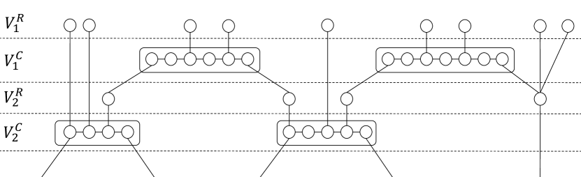
Figure 3: A decomposition satisfying the requirements in Lemma 2.9.

2.4 Descriptive combinatorics

Before we define formally the descriptive combinatorics complexity classes, we give a high-level overview on their connection to distributing computing for the readers more familiar with the latter.

The complexity class that partially captures deterministic local complexity classes and hints the additional computation power that one can gets in the infinite setting is called $\mathsf{BOREL}$. First, by a result of Kechris, Solecki and Todorčević [KST99] the maximal independent set problem is in this class for any bounded degree graph. In particular, this yields that $\mathsf{BOREL}$ contains the class $\mathsf{LOCAL}(O(\log^{*}n))$ by the characterization of [CKP19], see [Ber20a]. Moreover, (see the definition below) $\mathsf{BOREL}$ is closed under countably many iterations of the operations of finding a maximal independent set in some power of the graph, and of applying a constant local rule that takes into account what has been constructed previously. Therefore, the constructions in the class $\mathsf{BOREL}$ can use some unbounded, global, information.

The “truly” local class in descriptive combinatorics is the class $\mathsf{CONTINUOUS}$. As above the inclusion $\mathsf{LOCAL}(O(\log^{*}n))\subseteq\mathsf{CONTINUOUS}$ holds in most reasonable classes of bounded degree graphs since it is possible to solve the maximal independent set problem in a continuous manner, see [Ber20a]. In the paper [Ber21], Bernshteyn showed that, in the context of Cayley graphs of countable groups, this class admits various equivalent definitions and the inclusion is in fact equality.

Another complexity class that we consider in this paper is the class $\mathsf{BAIRE}$. This is a topological relaxation of the class $\mathsf{BOREL}$, namely, a LCL is in the class $\mathsf{BAIRE}$ if there is a Borel solution that can be incorrect on a topologically negligible set. The main advantage of the class $\mathsf{BAIRE}$ is that it admits a hierarchical decomposition that is called toast. The independence of colorings on a tree together with this structure allows for a combinatorial characterization of the class $\mathsf{BAIRE}$, which was proven by Bernshteyn [Ber], see also Section 4.

Basic definitions

A Polish space is a separable, completely metrizable topological space. A prime example of a Polish space is the real numbers. A Polish space is called zero-dimensional if it admits a basis consisting of clopen sets. The two most important examples of zero-dimensional Polish spaces are the collection of irrational numbers (as a subspace of $\mathbb{R}$) and the Cantor set. In fact, the former captures the structure of general zero-dimensional Polish spaces, while the latter captures the structure of compact ones; essentially, one can always imagine that we are working on one of these spaces. Recall that the collection of Borel subsets of a topological space is the minimal family of sets which contains all open sets and closed under taking complements and countable unions. The family of Borel sets has sufficient closure properties so that most of the simply defined sets are contained in them. On the other hand, Borel sets still behave intuitively, that is, their category does not exhibit the paradoxes arising from the Axiom of Choice (e.g., Banach-Tarski). Since a graph on a space $X$ can be identified with a subset of $X^{2}$, we can talk about a graph being closed or Borel etc.

Recall that in a topological space $(X,\tau)$, a set $C\subseteq X$ is $\tau$-meager (or meager if the topology is clear) if it can be covered by countably many $\tau$-closed sets with empty interior. In Polish spaces, the collection of meager sets form a $\sigma$-ideal, [Kec95, Section 8]. This provides the notion of small sets in the same way as does the $\sigma$-ideal of null sets in measure spaces. A set $C\subseteq X$ is comeager if $X\setminus C$ is meager. Let $X$ be a standard Borel space, we say that a Polish topology $\tau$ on $X$ is compatible if the fixed original $\sigma$-algebra on $X$ and the $\tau$-Borel $\sigma$-algebra are the same.

We refer the reader to [Pik21, KM20, Ber20a, Kec95], or to [GR21a, Introduction, Section 4.1] and [GR21b, Section 7.1, 7.2] for intuitive examples and standard facts of descriptive set theory.

2.4.1 $\mathsf{CONTINUOUS}$

Let $X$ be a zero-dimensional Polish space. We follow Bernshteyn [Ber21, Section 2] and say that a graph $\mathcal{G}\subseteq X\times X$ is a continuous graph, if the neighborhood $N_{\mathcal{G}}(U)$ of any clopen set $U$ is clopen.

Definition 2.10 (Continuous Tree).

A continuous ($\Delta$-regular) tree $\mathcal{T}$ on $X$ is an acyclic $\Delta$-regular continuous graph. We define $\mathcal{H}(\mathcal{T})$ to be the set of all half-edges of $\mathcal{T}$.

The set $\mathcal{H}(\mathcal{T})$ carries a canonical zero-dimensional Polish topology inherited from $X$, namely, every pair of clopen sets $U,V\subseteq X$ determines a clopen set $(U\times V)\cap\mathcal{T}$ in the space $\mathcal{H}(\mathcal{T})$, where $\mathcal{H}(\mathcal{T})$ can be thought of as a set of ordered edges. Another concrete way how to describe the topology is as follows. By [Ber21, Lemma 2.3], we find a continuous vertex coloring of $\mathcal{T}$ such that vertices at distance at most $2$ are assigned different colors from some finite set $I$. Then $\mathcal{H}(\mathcal{T})$ can be defined as a disjoint union of clopen sets of the form $X_{(i,j)}$, where $i\not=j\in I$ and $X_{(i,j)}$ are half-edges adjacent to $i$-colored vertices that point towards $j$-colored vertices.

Definition 2.11 ($\mathsf{CONTINUOUS}$).

Let $\Pi=(\Sigma,\mathcal{V},\mathcal{E})$ be an LCL. We say that $\Pi$ is in the class $\mathsf{CONTINUOUS}$ if for every continuous tree $\mathcal{T}$ there is a continuous function $f:H(\mathcal{T})\to\Sigma$ that is a $\Pi$-coloring of $\mathcal{T}$.

We remark that this definition of the class $\mathsf{CONTINUOUS}$ is different than the one given in the introduction (intuitive description of the $\{0,1\}$-model). In Section 3, we show that these definitions coincide. In the next paragraphs, we describe particular instances of continuous trees.

The space of labelings

Recall that $T_{\Delta}$ is the $\Delta$-regular tree and we pick a distinguished vertex $\mathfrak{r}$ which we call the root. We write $\operatorname{Aut}(T_{\Delta})$ for the group of all automorphisms of $T_{\Delta}$ and $\operatorname{Aut}^{o}(T_{\Delta})$ for the subgroup that fixes $\mathfrak{r}$. Endowed with pointwise-convergence, or equivalently, subspace topology form ${T_{\Delta}}^{T_{\Delta}}$, $\operatorname{Aut}(T_{\Delta})$ is a Polish group and $\operatorname{Aut}^{o}(T_{\Delta})$ is a compact subgroup with countable index (see, [Gao08, Theorem 2.4.4]). We write $\operatorname{id}_{T_{\Delta}}$ for the identity in $\operatorname{Aut}(T_{\Delta})$.

For a set $b$, we define $b^{T_{\Delta}}$ to be the space of all $b$-labelings of vertices of $T_{\Delta}$. We endow $b^{T_{\Delta}}$ with the product topology, where $b$ is viewed as a discrete space. The shift action $\operatorname{Aut}(T_{\Delta})\curvearrowright b^{T_{\Delta}}$ is defined as

$$g\cdot x(v)=x(g^{-1}(v)),$$

where $g\in\operatorname{Aut}(T_{\Delta})$, $x\in b^{T_{\Delta}}$ and $v\in T_{\Delta}$.

Definition 2.12.

Write $b^{T_{\Delta}}/\sim$ for the quotient space of the action $\operatorname{Aut}^{o}(T_{\Delta})\curvearrowright b^{T_{\Delta}}$. That is, $x\sim y$ if and only if there is $g\in\operatorname{Aut}^{o}(T_{\Delta})$ so that $g\cdot x=y$. Given $x\in b^{T_{\Delta}}$, we let $[x]\in b^{T_{\Delta}}/\sim$ to be the $\sim$-equivalence class of $x$.

The graph $\mathcal{G}_{b,\Delta}$ on $b^{T_{\Delta}}/\sim$ is defined as follows: $[x]$ and $[y]$ form an edge in $\mathcal{G}_{b,\Delta}$ if and only if for every $z\in[x]$ there is a $g\in\operatorname{Aut}(T_{\Delta})$ that moves the root to one of its neighbors so that $g\cdot z\in[y]$.

It is easy to see that $\mathcal{G}_{b,\Delta}$ is not a continuous tree, as it contains cycles and even loops. For convenience, we extend the notion of a continuous graph to this setting.

Proposition 2.13.

The quotient space $b^{T_{\Delta}}/\sim$ is a compact zero-dimensional Polish space and the graph $\mathcal{G}_{b,\Delta}$ is a continuous graph of degree at most $\Delta$.

Proof.

The space $b^{T_{\Delta}}$ is a compact metric space. Write $d$ for the standard compatible metric, that is, $d(x,y)=2^{-k-1}$ if the first vertex where $x$ and $y$ differ is at a distance $k$ from the root $\mathfrak{r}$. It is a standard fact that the action $\operatorname{Aut}^{o}(T_{\Delta})\curvearrowright b^{T_{\Delta}}$ is continuous. Define the metric $d/\sim$ on $b^{T_{\Delta}}/\sim$ as

$$d/\sim([x],[y])=\inf\{d(x^{\prime},y^{\prime}):x^{\prime}\in[x],\ y^{\prime}\in[y]\}$$

where $x,y\in b^{T_{\Delta}}$. Equivalently, $d/\sim([x],[y])=2^{-k-1}$ is the minimal $k\in\mathbb{N}$ so that $x$ and $y$ do not have isomorphic labeled $k$-neighborhood of $\mathfrak{r}$. As $\operatorname{Aut}^{o}(T_{\Delta})$ is compact, we have that $d/\sim([x],[y])=0$ if and only if $[x]=[y]$. It is routine to verify that $d/\sim$ is a compatible metric for the quotient topology and that a clopen basis is given by labeled $k$-neighborhoods of $\mathfrak{r}$ considered up to isomorphism. This shows that $b^{T_{\Delta}}/\sim$ is a compact zero-dimensional Polish space.

The root $\mathfrak{r}$ of $T_{\Delta}$ has exactly $\Delta$-many neighbours. Let $g_{1},\dots,g_{\Delta}\in\operatorname{Aut}(T_{\Delta})$ be such that $g_{i}$ moves $\mathfrak{r}$ to its $i$-th neighbour. Then for every other $h\in\operatorname{Aut}(T_{\Delta})$ that moves $\mathfrak{r}$ to one of the neighbors, there is an $h^{\prime}\in\operatorname{Aut}^{o}(T_{\Delta})$ so that $h^{\prime}\cdot h=g_{i}$ for some $i\leq\Delta$. Consequently, the degree of $\mathcal{G}_{b,\Delta}$ is at most $\Delta$.

It is routine to verify that if $U$ is a basic clopen set, that is, a set defined by some $b$-labeling of a $k$-neighborhood of $\mathfrak{r}$ for some $k\in\mathbb{N}$, then $N_{\mathcal{G}_{b,\Delta}}(U)$, the neighborhood of $U$ in $\mathcal{G}_{b,\Delta}$, is a union of some $b$-labeled $(k+1)$-neighborhoods of $\mathfrak{r}$, thus a clopen set. ∎

The compact continuous tree $\mathcal{T}^{\operatorname{dist}}_{\Delta}$

First, we restrict our attention to labelings that satisfy local constraints. This way, we define a continuous tree that provides a bridge between local algorithms and the class $\mathsf{CONTINUOUS}$, see [Ber21, Section 5.A.]. Let $k\in\mathbb{N}$ and write $\ell_{k}$ for the size of the $k$-neighborhood of the root $\mathfrak{r}$ in $T_{\Delta}$, that is, $\ell_{k}=|B(\mathfrak{r},k)|=1+\Delta\sum_{i=0}^{k-1}(\Delta-1)^{i}$. By a simple greedy algorithm, we see that there exist $k$-distance colorings of $G$ with $\ell_{k}$ many colors for each $k\in\mathbb{N}$. Write $T^{[k]}_{\Delta}$ for the space of all $k$-distance colorings, we have $T^{[k]}_{\Delta}\subseteq\ell_{k}^{T_{\Delta}}$. Define $\mathcal{G}^{[k]}_{\Delta}$ to be the restriction of $\mathcal{G}_{\ell_{k},\Delta}$ to the quotient space $T^{[k]}_{\Delta}/\sim$.

Proposition 2.14.

The space $T^{[k]}_{\Delta}/\sim$ is a nonempty compact zero-dimensional Polish space and the graph $\mathcal{G}^{[k]}_{\Delta}$ is a $\Delta$-regular continuous graph of girth at least $k$.

Proof.

It is easy to see that $T^{[k]}_{\Delta}$ is $\operatorname{Aut}(T_{\Delta})$-invariant and closed in $\ell_{k}^{T_{\Delta}}$. Consequently, $T^{[k]}_{\Delta}/\sim$ is a nonempty compact zero-dimensional Polish space. By Proposition 2.13, we have that $\mathcal{G}^{[k]}_{\Delta}$ is a continuous graph as it is the restriction of $\mathcal{G}_{\ell_{k},\Delta}$ to $T^{[k]}_{\Delta}/\sim$. Suppose that there is a nontrivial cycle $[x_{1}],\dots,[x_{\ell}]$ in $\mathcal{G}^{[k]}_{\Delta}$. That is, $[x_{1}]=[x_{\ell}]$ and $([x_{i}],[x_{i+1}])\in\mathcal{G}^{[k]}_{\Delta}$ for every $i<\ell$. We may assume that $[x_{i}]\not=[x_{j}]$ for every $i<j<\ell$. By the definition and induction, the composition of the elements of $\operatorname{Aut}(T_{\Delta})$ that witness the edge relation in $\mathcal{G}_{\ell_{k},\Delta}$ map $\mathfrak{r}$ to a vertex of distance $\ell$ from $\mathfrak{r}$. If $\ell\leq k$, then these vertices have different labels, thus $[x_{1}]\not=[x_{\ell}]$. A similar argument shows that $\mathcal{G}^{[k]}_{\Delta}$ is $\Delta$-regular. ∎

Observe that $\operatorname{Aut}(T_{\Delta})$ acts on $\prod_{k\in\mathbb{N}}T^{[k]}_{\Delta}$ by the product shift action, that is, $(g\cdot x)_{k}(v)=x_{k}(g^{-1}(v))$ for every $x=(x_{k})_{k\in\mathbb{N}}\in\prod_{k\in\mathbb{N}}T^{[k]}_{\Delta}$ and $g\in\operatorname{Aut}(T_{\Delta})$.

Definition 2.15.

Define $X=\left(\prod_{k\in\mathbb{N}}T^{[k]}_{\Delta}\right)/\sim$, where $\sim$ is the equivalence relation induced by a restriction of the product shift action to $\operatorname{Aut}(T_{\Delta})^{o}$. Similarly, we abuse the notation and write $[{-}]$ for the corresponding equivalence classes. Let the graph $\mathcal{T}^{\operatorname{dist}}_{\Delta}$ be defined as follows: $[x],[y]\in X$ form an edge in $\mathcal{T}^{\operatorname{dist}}_{\Delta}$ if and only if there is $g\in\operatorname{Aut}(T_{\Delta})$ that moves $\mathfrak{r}$ to one of its neighbors and $(g\cdot x)\in[y]$.

A similar reasoning as in Proposition 2.13 yields the following.

Claim 2.16.

The sets of the form $\{[(x_{k})_{k\in\mathbb{N}}]\in X:\forall k\leq N\ x_{k}\restriction B(\mathfrak{r},N)=s_{k}\}$ form a basis in $X$, where $N\in\mathbb{N}$ and $s_{k}:B(\mathfrak{r},N)\to\ell_{k}$ for each $k\leq N$.

Proposition 2.17.

The space $X$ is a nonempty compact zero-dimensional Polish space and the graph $\mathcal{T}^{\operatorname{dist}}_{\Delta}$ is a continuous tree.

Proof.

Let $K\in\mathbb{N}$. Analogously to $X$ and $\mathcal{T}^{\operatorname{dist}}_{\Delta}$, we define the space $X_{K}=\left(\prod_{k\in K}T^{[k]}_{\Delta}\right)/\sim$ and graph $\mathcal{T}^{\operatorname{dist}}_{K}$. A similar argument as in the proof of Proposition 2.14 shows that $X_{K}$ is a nonempty zero-dimensional Polish space and $\mathcal{T}^{\operatorname{dist}}_{K}$ is a continuous graph of girth at least $K$.

Given $K_{0}<K_{1}\in\mathbb{N}$, there is a canonical continuous and surjective map $q_{K_{0},K_{1}}:X_{K_{1}}\to X_{K_{0}}$ that is a homomorphism from $\mathcal{T}^{\operatorname{dist}}_{K_{1}}$ to $\mathcal{T}^{\operatorname{dist}}_{K_{0}}$. It is routine to check that $X$ and $\mathcal{T}^{\operatorname{dist}}_{\Delta}$ are inverse limits of the systems $(X_{K})_{K\in\mathbb{N}}$ and $(\mathcal{T}^{\operatorname{dist}}_{K})_{K\in\mathbb{N}}$. This gives all the desired properties. ∎

The universal continuous tree $\mathcal{T}^{\operatorname{\{0,1\}}}_{\Delta}$

In the next example, we consider the space of $\{0,1\}$-labelings of $T_{\Delta}$ that breaks all symmetries. This model has been studied extensively in the literature, see [GJS09, STD16, GJKS18, Ber21], in the case of countable groups and their Cayley graphs. The main difference from the previous example is that these continuous graphs are not defined on a compact spaces.

Definition 2.18.

Let $\operatorname{Free}\left(\{0,1\}^{T_{\Delta}}\right)$ be the set of all elements of $\{0,1\}^{T_{\Delta}}$ that break all the symmetries of $T_{\Delta}$. That is, $x\in\operatorname{Free}\left(\{0,1\}^{T_{\Delta}}\right)$ if and only if $g\cdot x\not=x$ whenever $\operatorname{id}_{T_{\Delta}}\not=g\in\operatorname{Aut}(T_{\Delta})$.

It is easy to see that the space $\operatorname{Free}\left(\{0,1\}^{T_{\Delta}}\right)$ is $\operatorname{Aut}(T_{\Delta})$-invariant, however, it is not obvious that it is nonempty. On the other hand, if it is nonempty, then it is again not difficult to see that it is not compact.

Definition 2.19.

Let $\mathcal{T}^{\operatorname{\{0,1\}}}_{\Delta}$ be the restriction of $\mathcal{G}_{\{0,1\},\Delta}$ to the set $\operatorname{Free}(\{0,1\}^{T_{\Delta}})/\sim$.

Proposition 2.20.

The space $\operatorname{Free}\left(\{0,1\}^{T_{\Delta}}\right)/\sim$ is a nonempty zero-dimensional Polish space and the graph $\mathcal{T}^{\operatorname{\{0,1\}}}_{\Delta}$ is a continuous tree.

Proof.

By [Kec95, Theorem 3.11], it is clearly enough to show that $\operatorname{Free}\left(\{0,1\}^{T_{\Delta}}\right)$ is a nonempty $G_{\delta}$-subset of $\{0,1\}^{T_{\Delta}}$. It is not hard to verify that $x\in\operatorname{Free}\left(\{0,1\}^{T_{\Delta}}\right)$ if and only if for every $v\not=w\in T_{\Delta}$ there is $k\in\mathbb{N}$ so that $x\upharpoonright B(v,k)$ and $x\upharpoonright B(w,k)$ are not isomorphic. The latter condition is clearly $G_{\delta}$. To show that $\operatorname{Free}\left(\{0,1\}^{T_{\Delta}}\right)$ is nonempty, we can simply consider a random element of $\{0,1\}^{T_{\Delta}}$ with respect to the product coin-flip measure. ∎

2.4.2 $\mathsf{BOREL}$

Let $X$ be a standard Borel space. A partial Borel isomorphism $\varphi$ of $X$ is a Borel bijection defined between two Borel subsets of $X$, $\operatorname{dom}(\varphi)$ and $\operatorname{rng}(\varphi)$. For a finite collection $\Phi=(\varphi_{i})_{i\in I}$ of partial Borel isomorphisms, we define a graph $\mathcal{G}_{\Phi}$ as $(x,y)\in\mathcal{G}_{\Phi}$ if there is $i\in I$ so that $\varphi_{i}(x)=y$ or $\varphi_{i}(y)=x$. Every graph $\mathcal{G}_{\Phi}$ defined in this manner is called a Borel graph.

Definition 2.21 (Borel Tree).

A Borel ($\Delta$-regular) tree $\mathcal{T}$ is an acyclic $\Delta$-regular Borel graph. We define $\mathcal{H}(\mathcal{T})$ to be the set of all half-edges of $\mathcal{T}$. Formally, this is the set of all pairs $(x,i)$, where $\Phi=(\varphi)_{i\in I}$ is the collection that defines $\mathcal{T}$, $x\in\operatorname{dom}(\varphi_{i})$ and $i\in I$.

The space $\mathcal{H}(\mathcal{T})$ is naturally endowed with a standard Borel structure, i.e., it is a disjoint union of finitely many Borel sets.

Definition 2.22 ($\mathsf{BOREL}$).

Let $\Pi=(\Sigma,\mathcal{V},\mathcal{E})$ be an LCL. We say that $\Pi$ is in the class $\mathsf{BOREL}$ if for every Borel tree $\mathcal{T}$ there is a Borel function $f:H(\mathcal{G})\to\Sigma$ that is a $\Pi$-coloring of $\mathcal{T}$.

It is a standard fact, see [Kec95, Section 13], that given a finite collection of partial Borel isomorphism on $X$, one can find a compatible zero-dimensional Polish topology that turns them into partial homeomorphisms. This gives immediately the following result.

Theorem 2.23.

Let $\Pi$ be an LCL. If $\Pi\in\mathsf{CONTINUOUS}$, then $\Pi\in\mathsf{BOREL}$.

2.4.3 $\mathsf{BAIRE}$

Now, we are ready to define the class $\mathsf{BAIRE}$ as the relaxation of the class $\mathsf{BOREL}$.

Definition 2.24 ($\mathsf{BAIRE}$).

Let $\Pi=(\Sigma,\mathcal{V},\mathcal{E})$ be an LCL. We say that $\Pi$ is in the class $\mathsf{BAIRE}$ if for every Borel tree $\mathcal{T}$ on a standard Borel space $X$ and every compatible Polish topology $\tau$ on $X$, there is a Borel function $f:H(\mathcal{T})\to\Sigma$ that is a $\Pi$-coloring of $\mathcal{T}$ on a $\tau$-comeager set.

An equivalent definition would require a function $f$ that is a $\Pi$-coloring everywhere but merely $\tau$-Baire measurable (measurable with respect to the smallest $\sigma$-algebra that contains Borel sets and $\tau$-meager sets). A direct consequence of the definitions is the following.

Theorem 2.25.

Let $\Pi$ be an LCL. If $\Pi\in\mathsf{BOREL}$, then $\Pi\in\mathsf{BAIRE}$.

Toast decomposition

The main technical advantage, that the class $\mathsf{BAIRE}$ offers, is the possibility of building a hierarchical decomposition. Finding a hierarchical decomposition in the context of descriptive combinatorics is tightly connected with the notion of Borel hyperfiniteness. Understanding which Borel graphs are Borel hyperfinite is a major theme in descriptive set theory [DJK94, GJ15, CJM⁺20]. It is known that grids, and generally polynomial growth graphs are hyperfinite, while, e.g., acyclic graphs are not in general hyperfinite [JKL02]. A strengthening of hyperfiniteness that is of interest to us is called toast [GJKS15, CM16].

Definition 2.26 (Toast).

Let $G$ be a graph and $q\in\mathbb{N}$. A $q$-toast of $G$ is a collection $\mathcal{D}$ of finite subsets of $G$ with the property that (i) every pair of vertices is covered by an element of $\mathcal{D}$ and (ii) the boundaries of every $D\not=E\in\mathcal{D}$ are at least $q$ apart in the graph distance.

Let $\mathcal{G}$ be a Borel graph on a standard Borel set $X$. A $q$-toast $\mathcal{D}$ of $\mathcal{G}$ is Borel, if it is a Borel subset of the standard Borel space of all finite subsets of $X$.

In the case of trees there is no way of constructing a Borel toast in general, however, it is a result of Hjorth and Kechris [HK96] that every Borel graph is hyperfinite on a comeager set for every compatible Polish topology. A direct consequence of [MU16, Lemma 3.1] together with a standard construction of a toast via Voronoi cells gives the following strengthening of toasts.

Proposition 2.27.

Let $\mathcal{G}$ be a Borel graph on a standard Borel space $X$ that has degree bounded by $\Delta\in\mathbb{N}$ and $\tau$ be a compatible Polish topology on $X$. Then for every $q>0$ there is a Borel $\mathcal{G}$-invariant $\tau$-comeager set $C$ on which $\mathcal{G}$ admits a Borel $q$-toast.

Proof.

Fix $q\in\mathbb{N}$ and a sufficiently fast growing function $f(n)$, e.g., $f(n)=(2q)^{n^{2}}$. Then [MU16, Lemma 3.1] gives a sequence $\{A_{n}\}_{n\in\mathbb{N}}$ of Borel subsets of $X$ such that $C=\bigcup_{n\in\mathbb{N}}A_{n}$ is a Borel $\tau$-comeager set that is $\mathcal{G}$-invariant, and $dist_{\mathcal{G}}(x,y)\geq f(n)$ for every distinct $x,y\in A_{n}$. We produce a toast structure in a standard way, e.g., see [GR21b, Appendix A].

Let $B_{n}(x)=B_{\mathcal{G}}(x,f(n)/3)$ and $R_{n}(x)=B_{\mathcal{G}}(x,f(n)/4)$, where $n\in\mathbb{N}$ and $x\in A_{n}$. Iteratively, define cells $\mathcal{D}_{n}=\{C_{n}(x)\}_{x\in A_{n}}$ as follows. Set $C_{1}(x)=R_{1}(x)$. Suppose that $\mathcal{D}_{n}$ has been defined and set

• $H^{n+1}(x,n+1):=R_{n+1}(x)$ for every $x\in A_{n+1}$,

• if $1\leq i\leq n$ and $\left\{H^{n+1}(x,i+1)\right\}_{x\in A_{n+1}}$ has been defined, then we put

  $$H^{n+1}(x,i)=\bigcup\left\{B_{i}(y):H^{n+1}(x,i+1)\cap B_{i}(y)\not=\emptyset\right\}$$

  for every $x\in A_{n+1}$,

• set $C_{n+1}(x):=H^{n+1}(x,1)$ for every $x\in A_{n+1}$, this defines $\mathcal{D}_{n+1}$.

The fact that $\mathcal{D}=\bigcup_{n\in\mathbb{N}}\mathcal{D}_{n}$ is a $q$-toast of $\mathcal{G}$ restricted to $C$ follows from the fact that $C=\bigcup_{n\in\mathbb{N}}A_{n}$ together with the fact that the boundaries are $q$ separated (see [GR21b, Appendix A] for more details). ∎

$\mathsf{TOAST}$ algorithm

The idea to use a toast structure to solve LCLs appears in [CM16] and has many applications since then [GJKS15, MU17]. This approach has been formalized in [GR21b], where the authors introduce $\mathsf{TOAST}$ algorithms. As we use this notion in Section 4, we discuss here briefly the definition and refer the reader to [GR21b, Section 4] for more details.

An LCL $\Pi$ admits a $\mathsf{TOAST}$ algorithm if there is $q\in\mathbb{N}$ and a partial extending function that has the property that whenever it is applied inductively to a $q$-toast, then it produces a $\Pi$-coloring. Recall that a partial extending function gets a finite subset of some underlying set that is partially colored as an input and outputs an extension of this coloring on the whole finite subset. An advantage of this approach is that once we know that a given Borel graph admits a Borel or Baire toast structure, and a given LCL $\Pi$ admits a $\mathsf{TOAST}$ algorithm, then we may conclude that $\Pi$ is in the class $\mathsf{BOREL}$ or $\mathsf{BAIRE}$, respectively.

2.5 The remaining implications on Fig. 1

Let us discuss now the arrows on Fig. 1 that are not the main two results of this paper. Note that assuming the two main results and using Theorem 2.6, we only have to show two things. First, that there is a descriptive class corresponding to $\mathsf{LOCAL}(O(1))$, second, that $\mathsf{CONTINUOUS}\subsetneq\mathsf{BOREL}\subsetneq\mathsf{BAIRE}$.

(a) In order to show that problems in $\mathsf{LOCAL}(O(1))$ can be defined purely in descriptive combinatorics terminology, we define the continuous tree $\mathcal{T}^{\mathbb{N}}_{\Delta}$. The vertex set are injective maps from $T_{\Delta}\to\mathbb{N}$, i.e., a closed and $\operatorname{Aut}(T_{\Delta})$-invariant subset of $T_{\Delta}^{\mathbb{N}}$, and $\mathcal{T}^{\mathbb{N}}_{\Delta}$ is the restriction of $\mathcal{G}_{\mathbb{N},\Delta}$ to this set. It is easy to verify that the class $\mathsf{LOCAL}(O(1))$ is the same as the class of problems solvable by uniformly continuous (for the cannical metric) function. It is interesting to note that from the perspective of $\mathsf{BOREL}$ is the graph $\mathcal{T}^{\mathbb{N}}_{\Delta}$ trivial, i.e, there is a Borel set that intersect every connected component of $\mathcal{T}^{\mathbb{N}}_{\Delta}$ in exactly one point. On the other hand we do not know if $\mathsf{CONTINUOUS}$ is equal to $\mathsf{LOCAL}(O(\log^{*}n))$ on this graph.

(b) It is proved in [BCG⁺21a] that the $\Delta$-coloring problem with paths distinguishes the classes $\mathsf{CONTINUOUS}$ and $\mathsf{BOREL}$. Recall that to solve the problem we have to produce a $\Delta$-coloring but we are allowed not to color some vertices. The constraint is that the induced subgraph on the uncolored vertices consists of doubly infinite paths. The intuitive reason why this problem is not in $\mathsf{CONTINUOUS}$ is that it is not possible to produce doubly infinite lines in a continuous way. This is proved formally in [BCG⁺21a]. On the other hand, after inductively discarding $(\Delta-2)$-many Borel maximal independent sets, the induced subgraph on the remaining vertices consists of finite, one-ended, or doubly infinite paths. This is clearly enough to construct the desired solution in a Borel way.

Finally, [CMTD16] and [Mar16] show that $\Delta$-coloring distinguishes between $\mathsf{BOREL}$ and $\mathsf{BAIRE}$.

3 Continuous colorings

Now we turn to the investigation of the existence of continuous solutions of LCL’s on regular trees. Our main contribution is that, unlike in the main theorem of [Ber20a], we do not need to assume that our graph is given by a group action, that is, the edges do not come with a proper edge $\Delta$-coloring. As seen below, this requires a significant change of Bernshteyn’s argument.

Recall the definition of $\mathcal{T}^{\operatorname{dist}}_{\Delta}$ and $\mathcal{T}^{\operatorname{\{0,1\}}}_{\Delta}$ from Section 2.4.1.

Theorem 3.1.

Let $\Pi$ be an LCL on $\Delta$-regular trees. The following are equivalent:

1. $\Pi\in\mathsf{LOCAL}(O(\log^{*}n))$

2. $\Pi\in\mathsf{CONTINUOUS}$

3. $\Pi$ admits a continuous solution on $\mathcal{T}^{\operatorname{dist}}_{\Delta}$

4. $\Pi$ admits a continuous solution on $\mathcal{T}^{\{0,1\}}_{\Delta}$

It is clear that (2) implies (3) and (4). Before we turn our attention to the most challenging part (4) implies (2) (Theorem 3.4), we demonstrate that (1) implies (2) (Theorem 3.2), and (3) implies (1) (Theorem 3.3). These implications are fairly standard and almost follow from [Ber20a, Ele18, Ber21]. The reason why we cannot use these results directly is that we consider LCLs defined on half-edges.

Theorem 3.2 ([Ber20a]).

Let $\Pi$ be an LCL such that $\Pi\in\mathsf{LOCAL}(O(\log^{*}n))$. Then $\Pi\in\mathsf{CONTINUOUS}$.

Proof.

By the results of [CP19, CKP19], we have that $\Pi$ can be solved by an algorithm that first solves the $k$-distance coloring problem, for some $k\in\mathbb{N}$, and then a local algorithm $\mathcal{A}$ with complexity $O(1)$ is applied. We may assume that $k>2$.

Let $\mathcal{T}$ be a continuous tree on $X$. By [Ber21, Lemma 2.3], there is a continuous $k$-distance coloring $c$ of $\mathcal{T}$. As $k>2$, $c$ also defines a partition $\bigsqcup X_{i,j}=\mathcal{H}(\mathcal{T})$ into clopen sets, where $i\not=j\in\operatorname{rng}(c)$, and $X_{i,j}$ is the set of half-edges that point from $i$-colored vertices to $j$-colored vertices. Now, it is easy to see that composing $c$ with $\mathcal{A}$ defines a continuous map with domain $\mathcal{H}(\mathcal{T})$, and it is routine to check that it is a $\Pi$-coloring of $\mathcal{T}$. ∎

Theorem 3.3 ([Ele18, Ber21]).

Let $\Pi$ be an LCL such that $\mathcal{T}^{\operatorname{dist}}_{\Delta}$ admits a continuous $\Pi$-coloring. Then $\Pi\in\mathsf{LOCAL}(O(\log^{*}n))$.

Proof.

Suppose that $\varphi$ is a continuous $\Pi$-coloring of $\mathcal{T}^{\operatorname{dist}}_{\Delta}$. By Proposition 2.17 and the definition of the topology on $\mathcal{H}(\mathcal{T})$, there is some $N\in\mathbb{N}$ such that the value of $\varphi$ on the half-edges around $[(x_{k})_{k\in\mathbb{N}}]$ depends only on the isomorphism type of the restriction of $(x_{k})_{k\leq N}$ to $B_{\mathcal{T}^{\operatorname{dist}}_{\Delta}}(\mathfrak{r},N)$, where we recall that $\mathfrak{r}$ is the root of $T_{\Delta}$. Set $\mathcal{A}$ to be the local algorithm of complexity $O(1)$ that gets as an input isomorphism type of a neigborhood $B(\mathfrak{r},N)$ with a sequence of vertex labelings $(c_{k})_{k\leq N}$, where $c_{k}$ is a solution to the $k$-distance coloring problem on $B(\mathfrak{r},N)$ for every $k\leq N$, and outputs labeling of half-edges around $\mathfrak{r}$. Note that $\mathcal{A}$ is well defined by the properties of $\varphi$.

Given a finite regular tree $T$, we describe how to solve $\Pi$ in $O(\log^{*}n)$ rounds with deterministic local algorithm. The main technical difficulty is that $\mathcal{A}$ assumes as an input an isomorphic copy of the rooted graph $B(\mathfrak{r},N)$, therefore we need to trick the algorithm whenever it is applied to a vertex that is close to a virtual half-edge. Similar argument appeared in [Ber21, Section 5.3]. First, we produce a sequence $(c_{k})_{k\leq N}$ of vertex labelings that solve the $k$-distance coloring problem on $T$ for every $k\leq N$. As $N\in\mathbb{N}$ is fixed, this requires $O(\log^{*}n)$ rounds. Second, we construct a solution to the $2N$-distance coloring problem. Inductively along the color classes, we extend $T$ and $(c_{k})_{k\leq N}$ to a finite tree $T^{\prime}$ and $(c^{\prime}_{k})_{k\leq N}$ such that $c^{\prime}_{k}$ is a $k$-distance coloring of $T^{\prime}$ for very $k\leq N$, and $B_{T^{\prime}}(v,N)$ is isomorphic to $B(\mathfrak{r},N)$ for every $v\in V(T)$. Note that this is possible by a simple greedy algorithm as the number of colors that we can use to solve the $k$-distance coloring problem is $\ell_{k}=|B(\mathfrak{r},k)|$, and vertices in the same color class can do the extension independently as their distance is bigger than $2N$. This requires $O(\log^{*}n)+O(1)$ rounds. Finally, we apply $\mathcal{A}$ to the isomorphism type of $(c^{\prime}_{k}\upharpoonright B_{T^{\prime}}(v,N))_{k\leq N}$ at every vertex $v\in V(T)$. It is routine to verify that this produces a $\Pi$-coloring of $T$ in $O(\log^{*}n)$ rounds. ∎

3.1 The tree $\mathcal{T}^{\{0,1\}}_{\Delta}$

In order to finish the proof of Theorem 3.1, we have to show the following.

Theorem 3.4.

Assume that $\Pi$ admits a continuous solution on $\mathcal{T}^{\{0,1\}}_{\Delta}$ and $\mathcal{T}$ is a $\Delta$-regular continuous tree. Then $\Pi$ admits a continuous solution on $\mathcal{T}$.

Our strategy follows closely Bernshteyn’s argument [Ber21]. Namely, given a continuous tree $\mathcal{T}$ on $X$, we construct a continuous $\{0,1\}$-labeling of $X$ in such a way that the $\{0,1\}$-labeled tree rooted at any given vertex $x\in X$, i.e., the vertex labeled connected component of $x$ in $\mathcal{T}$, is “close” to $\operatorname{Free}\left(\{0,1\}^{T_{\Delta}}\right)$. Here “close” means that the continuous function on $\operatorname{Free}\left(\{0,1\}^{T_{\Delta}}\right)$ that solves $\Pi$ can be extended to these elements. Before we give a formal proof, we need to introduce some technical notation and recall the continuous Lovász Local Lemma of Bernshteyn [Ber21].

3.1.1 Hyperaperiodic elements

An element $[\alpha]\in\operatorname{Free}\left(\{0,1\}^{T_{\Delta}}\right)/\sim$ is called hyperaperiodic if the closure of the connectivity component of $[\alpha]$ in $\mathcal{T}^{\{0,1\}}_{\Delta}$ in the space $\{0,1\}^{T_{\Delta}}/\sim$ is a subset of $\operatorname{Free}\left(\{0,1\}^{T_{\Delta}}\right)/\sim$. Equivalently, the closure is a compact subset of $\operatorname{Free}\left(\{0,1\}^{T_{\Delta}}\right)/\sim$, or every element that can be approximated by a sequence from $\operatorname{Aut}(T_{\Delta})\cdot\alpha$ is in the space $\operatorname{Free}\left(\{0,1\}^{T_{\Delta}}\right)$. We also abuse the notation and say that $\alpha\in\operatorname{Free}\left(\{0,1\}^{T_{\Delta}}\right)$ is hyperaperiodic if $[\alpha]$ is such.

This notion is well studied in the context of countable groups [GJS09, STD16, GJKS18, Ber21]. Namely, every countable group $\Gamma$ admits such a $\{0,1\}$-labeling, in particular, every Cayley graph of finitely generated group $\Gamma$ admits such a coloring with respect to the shift action of $\Gamma$. As a byproduct of our main result, we show that these elements indeed exist even in our setting, where the automorphism group is much larger. It is an exciting open problem to understand for which other classes of (structured) graphs hyperaperiodic elements exist.

Theorem 3.5.

There are hyperaperiodic elements in $\operatorname{Free}\left(\{0,1\}^{T_{\Delta}}\right)/\sim$.

The statement follows from the last part of the proof of Theorem 3.4. The following is the main definition that we use to approximate hyperaperiodic elements.

Definition 3.6.

Let $g\in\operatorname{Aut}(T_{\Delta})$, $\alpha\in{\{0,1\}}^{T_{\Delta}}$, $v\in T_{\Delta}$, $n\in\mathbb{N}$ and $K\in\mathbb{N}$. We say that $(\alpha,K)$ $n$-breaks $g$ at $v$ if either $dist(g\cdot v,v)>n$ or $g\cdot v=v$, or $g\cdot\alpha^{\prime}\not=\alpha^{\prime}$ for every $\alpha^{\prime}\in\{0,1\}^{T_{\Delta}}$ such that

$$\alpha\upharpoonright B(v,K)=\alpha^{\prime}\upharpoonright B(v,K).$$

Define

$$X_{K,n}=\left\{\alpha\in\{0,1\}^{T_{\Delta}}:\forall v\in T_{\Delta},\forall g\in\operatorname{Aut}(T_{\Delta})\ (\alpha,K)\ n\operatorname{-breaks}\ g\ \operatorname{at}\ v\right\}$$

for every $K,n\in\mathbb{N}$.

Proposition 3.7.

Let $n>1$, $K\in\mathbb{N}$ and suppose that $X_{K,n}\subseteq\{0,1\}^{T_{\Delta}}$ is non-empty. The sets $X_{K,n}$ and $X_{K,n}/\sim$ are compact, $X_{K,n}$ is $\operatorname{Aut}(T_{\Delta})$-invariant and we have $dist(g\cdot v,v)>n$ for every $v\in T_{\Delta}$ and $\operatorname{id}_{T_{\Delta}}\not=g\in\operatorname{Aut}(T_{\Delta})$ that satisfies $g\cdot\alpha=\alpha$ for some $\alpha\in X_{K,n}$. In particular, $\mathcal{G}_{\{0,1\},\Delta}\upharpoonright(X_{K,n}/\sim)$ has girth at least $n$.

Proof.

It is easy to see from the definition that $X_{K,n}$ is $\operatorname{Aut}(T_{\Delta})$-invariant. Suppose that $\alpha_{\ell}\to\alpha$ in $\{0,1\}^{T_{\Delta}}$, where $\alpha_{\ell}\in X_{K,n}$ for every $\ell\in\mathbb{N}$. Let $v\in T_{\Delta}$ and $g\in\operatorname{Aut}(T_{\Delta})$. We need to show that $(\alpha,K)$ $n$-breaks $g$ at $v$. If not, then $0<dist(g\cdot v,v)\leq n$ and we find $\alpha^{\prime}\in\{0,1\}^{T_{\Delta}}$ such that $g\cdot\alpha^{\prime}=\alpha^{\prime}$ and $\alpha\upharpoonright B(v,K)=\alpha^{\prime}\upharpoonright B(v,K)$. Taking $\ell\in\mathbb{N}$ large so that $\alpha\upharpoonright B(v,K)=\alpha_{\ell}\upharpoonright B(v,K)$, we see that $(\alpha_{\ell},K)$ does not $n$-break $g$ at $v$ as well, a contradiction. This shows that $X_{K,n}$, and consequently $X_{K,n}/\sim$, is closed and hence compact.

Let $g\in\operatorname{Aut}(T_{\Delta})$ be such that $g\cdot\alpha=\alpha$ for some $\alpha\in X_{K,n}$. It is easy to see that if there is a $w\in T_{\Delta}$ such that $g\cdot w=w$, then either $g=\operatorname{id}_{T_{\Delta}}$, or we can find a $v\in T_{\Delta}$ such that $dist(g\cdot v,v)=2$. Altogether, if neither $g\not=\operatorname{id}_{T_{\Delta}}$ nor $dist(g\cdot v,v)>n$ hold for every $v\in T_{\Delta}$, then there is a $v\in T_{\Delta}$ so that $0<dist(g\cdot v,v)\leq n$. From the definition of $X_{K,n}$, we have that $(\alpha,K)$ $n$-breaks $g$ at $v$. But that contradicts the fact that $g\cdot\alpha=\alpha$, hence, $g=\operatorname{id}_{T_{\Delta}}$ or $dist(g\cdot v,v)>n$ for every $v\in T_{\Delta}$.

The additional part follows by the same argument as in Proposition 2.14, namely, if there were a non-trivial cycle in $\mathcal{G}_{\{0,1\},\Delta}\upharpoonright(X_{K,n}/\sim)$ of length at most $n$, then the composition of the elements of $\operatorname{Aut}(T_{\Delta})$ that witness the edge relations would produce a $g\in\operatorname{Aut}(T_{\Delta})$ that fixes some $\alpha\in X_{K,n}$ and satisfies $0<dist(g\cdot\mathfrak{r},\mathfrak{r})\leq n$, a contradiction. ∎

3.1.2 Continuous Lovász Local Lemma

In order to construct/approximate hyperaperiodic elements, Bernshteyn [Ber21] developed a continuous version of the Lovász Local Lemma (LLL). Namely, he found a sufficient LLL-style condition for the existence of a continuous solution to a continuous constraint satisfaction problem (CSP) defined on a zero-dimensional Polish space, see the definitions below. Rather surprisingly, a similar but incomparable sufficient condition for the existence of $O(\log^{*}n)$ deterministic algorithms was studied in the distributed computing literature [BGR20]. We note that both conditions are tight, see the discussion in [Ber21, Section 1.A.2].

Let $X$ be a set and $k\in\mathbb{N}$. For a finite set $D\subseteq X$, an $(X,k)$-bad event with domain $D$ is an element of $k^{D}$. A constraint $\mathscr{B}$ with domain $D$ is a collection of $(X,k)$-bad events with domain $D$; we will use the notation $\operatorname{dom}(\mathscr{B})=D$, and omit $X$ and $k$ if it is clear from the context. A CSP $\mathfrak{B}$ (on $X$ with range $k$) is a set of $(X,k)$-constraints. Define the maximal probability of $\mathfrak{B}$ as

$$p(\mathfrak{B})=\sup_{\mathscr{B}\in\mathfrak{B}}\frac{|\mathscr{B}|}{k^{|dom(\mathscr{B})|}},$$

the vertex degree of $\mathfrak{B}$ as

$$vdeg(\mathfrak{B})=\sup_{x\in X}|\{\mathscr{B}\in\mathfrak{B}:x\in dom(\mathscr{B})\}|,$$

and the order of $\mathfrak{B}$ by

$$ord(\mathfrak{B})=\sup_{\mathscr{B}\in\mathfrak{B}}|\operatorname{dom}(\mathscr{B})|.$$

If $X$ is a zero-dimensional Polish space, a CSP $\mathfrak{B}$ on $X$ is continuous if for every set $S$ of functions $\{1,\dots,n\}\to k$ and $U_{2},\dots,U_{n}\subseteq X$ clopen the set

$$\{x_{1}:\text{there are $x_{2}\in U_{2},\dots,x_{n}\in U_{n}$ such that }x_{1},\dots,x_{n}\text{ are distinct and }S(x_{1},\dots,x_{n})\in\mathfrak{B}\}$$

is clopen, where $S(x_{1},\dots,x_{n})$ stands for the collection of functions determined by the elements of $S$, i.e., $f\in S(x_{1},\dots,x_{n})$ if for some $\varphi\in S$ we have $f(x_{i})=j\iff\varphi(i)=j$.

A $k$-coloring $f:X\to k$ satisfies (or solves) the CSP $\mathfrak{B}$ if $f$ has no restriction that is a bad event. The following theorem has been proven in [Ber21]:

Theorem 3.8 ([Ber21]).

Let $X$ be a zero-dimensional Polish space, $k\in\mathbb{N}$, and $\mathfrak{B}$ be a continuous CSP on $X$ with range $k$ such that

$$p(\mathfrak{B})\cdot vdeg(\mathfrak{B})^{ord(\mathfrak{B})}<1.$$

Then $\mathfrak{B}$ admits a continuous solution.

3.1.3 The continuous tree $\mathcal{T}$

The aim of this section is to show that every continuous $\{0,1\}$-labeling of vertices of a continuous tree $\mathcal{T}$ naturally induces a continuous homomorphism from $\mathcal{T}$ to $\mathcal{G}_{\{0,1\},\Delta}$. The main technical difficulty is that there is no unified way how vertices of $\mathcal{T}$ “view” their connected component and its automorphism group. To overcome this difficulty we first break local symmetry by a proper edge coloring.

Proposition 3.9.

Let $\mathcal{T}$ be a continuous tree. There is a continuous map $\Theta_{\mathcal{T}}:\mathcal{H}(\mathcal{T})\to(2\Delta-1)$ that solves the proper edge coloring problem.

Proof.

This is a direct consequence of [KST99], or Theorem 3.2 combined with [Lin92], applied to the line graph of $\mathcal{T}$. Recall that a line graph of $\mathcal{T}$ is a graph with a vertex set equal to the edge set of $\mathcal{T}$, where two edges of $\mathcal{T}$ form an edge in the line graph if they share a vertex in $\mathcal{T}$. ∎

Let $\mathcal{T}$ be a continuous tree on $Z$, $\Theta_{\mathcal{T}}$ as above and $x\in Z$. Moreover, fix the canonical linear ordering on the set $(2\Delta-1)$ and some ordering of vertices of $T_{\Delta}$. Write $I_{x}$ for the isomorphism between the connectivity component of $x$ in $\mathcal{T}$ and $T_{\Delta}$ that is defined inductively along $k=dist_{\mathcal{T}}(x,{-})$ as follows:

1. $I_{x}$ sends $x$ to the root $\mathfrak{r}$ of $T_{\Delta}$,

2. Suppose that $I_{x}$ is defined on $B_{\mathcal{T}}(x,k)$ and $dist_{\mathcal{T}}(x,y)=k$ for some $y\in B_{\mathcal{T}}(x,k)$. Consider the linear ordering on $\{z\in Z:dist_{\mathcal{T}}(x,z)=k+1,\ dist_{\mathcal{T}}(y,z)=1\}$ induced by $\Theta_{\mathcal{T}}$, i.e., $z_{0}<z_{1}$ if $\Theta_{\mathcal{T}}((y,e_{0}))<\Theta_{\mathcal{T}}((y,e_{1}))$, where $e_{i}=\{y,z_{i}\}$ for $i<2$. Extend $I_{x}$ in such a way that it respects this ordering and the restriction of the one fixed on $T_{\Delta}$ on the corresponding vertices.

Similarly, we define the action of $\operatorname{Aut}(T_{\Delta})$ on the connectivity component of $x$ in $\mathcal{T}$ from the perspective of $x$. That is, we define $g\odot_{x}y=I^{-1}_{x}(g\cdot I_{x}(y))$, where $x,y\in Z$, $g\in\operatorname{Aut}(T_{\Delta})$ and $y$ is in the connectivity component of $x$.

Proposition 3.10.

Let $\mathcal{T}$ be a continuous tree on $Z$ and $\psi:Z\to\{0,1\}$ be a continuous function. Then the map $\widetilde{h}_{\psi}:Z\to\{0,1\}^{T_{\Delta}}$ defined as

$$\widetilde{h}_{\psi}(x)(v)=\psi(I^{-1}_{x}(v))$$

is continuous. Moreover, the induced map $h_{\psi}:Z\to\{0,1\}^{T_{\Delta}}/\sim$ is a continuous homomorphism from $\mathcal{T}$ to $\mathcal{G}_{\{0,1\},\Delta}$.

Proof.

It follows directly from the definitions that the map is well-defined. As $\Theta_{\mathcal{T}}$ and $\psi$ are continuous, it follows that $\widetilde{h}_{\psi}$ is continuous as well. To see this note that the values of $\Theta_{\mathcal{T}}$ and $\psi$ on $B_{\mathcal{T}}(x,\ell)$ fully determine $\widetilde{h}_{\psi}$ on $B_{\mathcal{T}}(x,\ell)$. The moreover part easily follows. ∎

Let us remark that $h_{\psi}$ remains the same for any continuous assignment $x\mapsto I_{x}$, where $I_{x}$ is an enumeration of the connected component of $x$.

3.1.4 Key Lemma

The following technical lemma is the key tool, which allows us to iteratively define a homomorphism. Following the terminology from [Ber21], recall that if $\mathcal{T}$ is a continuous tree on a space $Z$ and $s,M\in\mathbb{N}$, a set $C\subseteq Z$ is called s-syndetic if for every $x\in Z$ there exists a $y\in C$ with $dist_{\mathcal{T}}(x,y)\leq s$; a set $U\subseteq Z$ is called $M$-separated, if $dist_{\mathcal{T}}(x,y)>M$ for every distinct $x,y\in U$.

Lemma 3.11.

Let $\mathcal{T}$ be a continuous $\Delta$-regular tree on the space $Z$. For every $s,n\in\mathbb{N}$ there are $K,M\in\mathbb{N}$ such that for every decomposition of $Z=C_{0}\sqcup C\sqcup U$ into clopen sets such that $C$ is $s$-syndetic and $U$ is $M$-separated, and every $\varphi_{0}:C_{0}\to\{0,1\}$ that is continuous, there is a continuous extension map $\varphi:C_{0}\cup C\to\{0,1\}$ so that for every continuous map $\psi:Z\to\{0,1\}$ that extends $\varphi$ we have that $h_{\psi}(Z)\subseteq X_{K,n}/\sim$.

Proof.

Let $L\in\mathbb{N}$ be divisible by $48s$ and such that

$$\left(\frac{\sqrt{2s}}{(\Delta-1)^{L/16}}\right)^{L/{24s}}\cdot(\Delta^{17L+2n})^{2}<1.$$

We show that that taking $M=L$ and $K=6L+n$ satisfies the conclusion of the lemma.

We start by taking a maximal $L$-separated clopen subset $\mathcal{Z}$ in $\mathcal{T}$. Such a set exists by [Ber21, Lemma 2.2] when one replaces $\mathcal{T}$ with the $L$-power graph of $\mathcal{T}$ and observe that this graph is a continuous graph as well.

Claim 3.12.

Let $x\in Z$ and $g\in\operatorname{Aut}(T_{\Delta})$ be such that $0<dist_{\mathcal{T}}(g\odot_{x}x,x)\leq n$. Then there is a $z_{x,g}\in\mathcal{Z}$ that satisfies the following:

• $dist_{\mathcal{T}}(x,z_{x,g})<4L$,

• $dist_{\mathcal{T}}(g\odot_{x}z_{x,g},z_{x,g})>L$.

Moreover, we may assume that the assignment $(x,g)\mapsto z_{x,g}$, that is defined on a clopen subset of $Z\times\operatorname{Aut}(T_{\Delta})$, is continuous.

Proof.

As $g\not=\operatorname{id}_{T_{\Delta}}$, there exists an $x^{\prime}\in Z$ with $dist_{\mathcal{T}}(x,x^{\prime})=2L$ and $dist_{\mathcal{T}}(x^{\prime},g\odot_{x}x^{\prime})=4L+dist_{\mathcal{T}}(g\odot_{x}x,x)$: indeed, any $x^{\prime}\in Z$ with $dist_{\mathcal{T}}(x,x^{\prime})=2L$ and the property that the shortest path between $g\odot_{x}x^{\prime}$ and $x^{\prime}$ contains $x$ and $g\odot_{x}x$ is suitable. To find such an $x^{\prime}$, we use that $\Delta>2$. Take $x_{0},x_{1},x_{2}$ in distance $2L$ from $x$ such that the shortest paths from $x_{i}$ to $x$ are pairwise edge disjoint. Then there is some $i<3$ such that the shortest path between $x_{i}$ and $x$ and between $g\odot_{x}x_{i}$ and $g\odot_{x}x$ are both edge disjoint from the one between $x$ and $g\odot_{x}x$. Letting $x^{\prime}=x_{i}$ works. Now, by the maximality of $\mathcal{Z}$ we can pick a $z_{x,g}\in\mathcal{Z}$ with $dist_{\mathcal{T}}(x^{\prime},z_{x,g})\leq L$, which is clearly suitable.

To see the additional part, first note that $(x,g)\mapsto z_{x,g}$ is defined on $Z\times\bigcup_{g\in I}g\cdot\operatorname{Aut}^{o}(T_{\Delta})$, where $I\subseteq\operatorname{Aut}(T_{\Delta})$ is some finite set. The argument above depends on a finite neighborhood of $x$ in $\mathcal{T}$, namely, the neighborhood of radius $6L+n$. Similarly, we only need to know the ’action’ $\odot_{{-}}$, and consequently the proper edge coloring $\Theta_{\mathcal{T}}$ from Proposition 3.9, in a finite radius around $x$ in $\mathcal{T}$. As all the involved objects are either continuous or clopen, it follows that the assignment $(x,g)\mapsto z_{x,g}$ can be chosen to be continuous as required. ∎

Claim 3.13.

Let $z\in\mathcal{Z}$ and define the set

$$C_{z}=\{r\in Z:\exists g\in\operatorname{Aut}(T_{\Delta})\ \exists x\in Z\ z=z_{x,g}\ \text{ and }\ g\odot_{x}z=r\}.$$

Then we have $|C_{z}|\leq 2\Delta^{8L+n}$.

Proof.

Let $r\in C_{z}$ and $x,g$ be from the definition. Then we have

$$\begin{split}dist_{\mathcal{T}}(z,r)=dist_{\mathcal{T}}(z,g\odot_{x}z_{g,x})\leq&\ dist_{\mathcal{T}}(z,x)+dist_{\mathcal{T}}(x,g\odot_{x}x)+dist_{\mathcal{T}}(g\odot_{x}x,g\odot_{x}z)\\ \leq&\ 4L+n+4L\end{split}$$ (1)

by Claim 3.12. We are done by using the upper bound $|B_{\mathcal{T}}(z,8L+n)|\leq 2\Delta^{8L+n}$. ∎

In order to utilize Theorem 3.8, we define a CSP that is suitable in our situation and yields the desired extension $\varphi$. For $z\in Z$, let $B_{z}=B_{\mathcal{T}}(z,L/4)$, note that $B_{z}\cap B_{z^{\prime}}=\emptyset$ for every $z\neq z^{\prime}\in\mathcal{Z}$. We apply the Theorem 3.8 with $X=\mathcal{Z}$ and $k=2^{|B_{z}|}$ for some, or equivalently any, $z\in\mathcal{Z}$. We use the proper edge coloring $\Theta_{\mathcal{T}}$ from Proposition 3.9 to identify $2^{B_{z}}$ with $k$ for each $z\in\mathcal{Z}$ in such a way that every continuous function $f:\mathcal{Z}\to k$ naturally encodes a continuous $\{0,1\}$-labelling of $\bigcup_{z\in\mathcal{Z}}B_{z}$.

Define $\varphi^{\prime}$ on the set $C_{0}\cup(C\setminus\bigcup_{z\in\mathcal{Z}}B_{z})$ to be $\varphi_{0}$ on $C_{0}$ and $0$ otherwise. Given a continuous map $f:\mathcal{Z}\to k$, we define $\varphi_{f}:C_{0}\cup C\to\{0,1\}$ to be the union of $\varphi^{\prime}$ and the $\{0,1\}$-labelling encoded by $f$ restricted to $C\cap\setminus\bigcup_{z\in\mathcal{Z}}B_{z}$. It is routine to verify that $\varphi^{\prime}$ is a continuous map defined on a clopen subset of $Z$. Similarly, $\varphi_{f}$ is continuous whenever $f$ is continuous. Next, we use Theorem 3.8 to find a suitable $f$ so that $\varphi:=\varphi_{f}$ has all the desired properties.

We define our CSP $\mathfrak{B}$. Given $z\in\mathcal{Z}$ and $r\in C_{z}$, we define the constraint $\mathcal{B}_{z,r}\in\mathfrak{B}$ with domain

$$\operatorname{dom}(\mathcal{B}_{z,r})=\left\{z^{\prime}\in\mathcal{Z}:B_{z^{\prime}}\cap\left(B_{z}\cup B_{r}\right)\right\}$$

as follows:

• $b:\operatorname{dom}(\mathcal{B}_{z,r})\to k$ is in $\mathcal{B}_{z,r}$ if and only if there is a $g\in\operatorname{Aut}(T_{\Delta})$ such that

  • $g\odot_{z}z=r$,

  • there is a labeling $\phi$ of $B_{z}\cup B_{r}$, which agrees with the labeling defined on $(B_{z}\cup B_{r})\setminus U$ by $\varphi^{\prime}$ and the $\{0,1\}$-labeling encoded by $b$ restricted to $C\cap(B_{z}\cup B_{r})$, such that for every $y\in B_{z}$ we have $\phi(y)=\phi(g\odot_{z}y)$.

It is not hard to see that $\mathfrak{B}$ is a continuous CSP. Let us argue first that it is sufficient to solve $\mathfrak{B}$ to show the lemma.

Claim 3.14.

Assume that $f:\mathcal{Z}\to k$ is a continuous solution to $\mathfrak{B}$. Then $\varphi_{f}$ satisfies the conclusion of Lemma 3.11.

Proof.

Let $\psi$ be a continuous extension of $\varphi_{f}$ to $Z$ and $x\in Z$. We show that $\widetilde{h}_{\psi}(x)\in X_{K,n}$. If not, then there are $v\in T_{\Delta}$ and $g\in\operatorname{Aut}(T_{\Delta})$ such that $(\widetilde{h}_{\psi}(x),K)$ does not $n$-break $g$ at $v$. By the definition, this means that $0<dist(g\cdot v,v)\leq n$ and there is an $\alpha\in\{0,1\}^{T_{\Delta}}$ such that $g\cdot\alpha=\alpha$ and $\widetilde{h}_{\psi}(x)\restriction B(v,K)=\alpha\restriction B(v,K)$.

We may assume that $v=\mathfrak{r}$, otherwise we replace $x$ with $I^{-1}_{x}(v)$. Let $z_{x,g}$ be from Claim 3.12 and set $r=g\odot_{x}z_{x,g}$. Recall that $K=6L+n$. Then we have

$$B_{r}\cup\bigcup_{z^{\prime}\in\operatorname{dom}(\mathcal{B}_{z,r})}B_{z^{\prime}}\subseteq B_{\mathcal{T}}(x,6L+n)$$ (2)

by Claim 3.12.

Set $b=f\upharpoonright\operatorname{dom}(\mathcal{B}_{z,r})$. We show that $b\in\mathcal{B}_{z,r}$ contradicting the assumption on $f$. For $u\in T_{\Delta}$ define $g_{0}\in\operatorname{Aut}(T_{\Delta})$ by

$$g_{0}\cdot u=I_{z}\circ I^{-1}_{x}(g\cdot(I_{x}\circ I^{-1}_{z})(u))=I_{z}(g\odot_{x}(I^{-1}_{z}(u))).$$

We have,

• by the definition of $g_{0}$, that $g_{0}\odot_{z}z=I^{-1}_{z}(g_{0}\cdot I_{z}(z))=g\odot_{x}z=r$,

• by $g\cdot\alpha=\alpha$ and the definition of $g_{0}$, that

  $$\begin{split}\alpha(I_{x}(y))=&\ \alpha(g\cdot I_{x}(y))=\alpha(g\cdot I_{x}(I_{z}^{-1}(I_{z}(y))))\\ =&\ \alpha(I_{x}\circ I_{z}^{-1}(g_{0}\cdot I_{z}(y)))\\ =&\ \alpha(I_{x}(g_{0}\odot_{z}y))\end{split}$$ (3)

  for $y\in B_{z}$,

• by (2), that $\phi=\alpha\circ I_{x}$ agrees with the labelling defined on $(B_{z}\cup B_{r})\setminus U$ by $\varphi^{\prime}$ and the $\{0,1\}$-labeling encoded by $b$ restricted to $C\cap(B_{z}\cup B_{r})$.

Consequently, $b\in\mathcal{B}_{z,r}$ and we are done. ∎

Claim 3.15.

We have $ord(\mathfrak{B})\leq 2$ and $vdeg(\mathfrak{B})\leq\Delta^{17L+2n}$.

Proof.

Let $z\in\mathcal{Z}$ and $r\in C_{z}$. Clearly, $z\in\operatorname{dom}(\mathcal{B}_{z,r})$. Suppose that $z_{0},z_{1}\in\operatorname{dom}(\mathcal{B}_{z,r})\setminus\{z\}$. By the definition of $\mathcal{Z}$, we have $B_{z_{i}}\cap B_{z}=\emptyset$, and therefore $B_{z_{i}}\cap B_{r}\not=\emptyset$ for $i\in\{0,1\}$. This implies that $dist_{\mathcal{T}}(z_{0},z_{1})<L$. Consequently, $z_{0}=z_{1}$ as $\operatorname{dom}(\mathcal{B}_{z,r})\subseteq\mathcal{Z}$.

Let $z\in\mathcal{Z}$. There are at most $2\Delta^{8L+n}$-many constraints of the form $\mathcal{B}_{z,r}$ by Claim 3.13. On the other hand, if $z\in\operatorname{dom}(\mathcal{B}_{z^{\prime},r^{\prime}})$ for some $z\not=z^{\prime}\in\mathcal{Z}$ and $r^{\prime}\in C_{z^{\prime}}$, then

$$dist_{\mathcal{T}}(z,z^{\prime})\leq dist_{\mathcal{T}}(z,r)+dist_{\mathcal{T}}(r,z^{\prime})\leq 8L+n+L/2$$

by (1). This shows that there are at most $2\Delta^{8L+n+L/2}$-many choices for $z^{\prime}\in\mathcal{Z}$, each having $2\Delta^{8L+n}$-many choices for $r^{\prime}\in C_{z^{\prime}}$. Altogether we have $vdeg(\mathfrak{B})\leq\Delta^{17L+2n}$ as desired. ∎

It remains to estimate $p(\mathfrak{B})$. Let $z\in\mathcal{Z}$ and $r\in C_{z}$. Set $\mathbb{P}(\mathcal{B}_{z,r})=\frac{|\mathcal{B}_{z,r}|}{k^{|\operatorname{dom}(\mathcal{B}_{z,r})|}}$, i.e., the probability that $b\in k^{\operatorname{dom}(\mathcal{B}_{z,r})}$ chosen uniformly at random falls into $\mathcal{B}_{z,r}$. With this notation we have

$$p(\mathfrak{B})=\sup_{z,r}\mathbb{P}(\mathcal{B}_{z,r}).$$

We start with a simple observation about the $s$-syndetic set $C$. For $x\in Z$ and $i\in\mathbb{N}$, we define $S_{\mathcal{T}}(x,i)=\{y\in Z:dist_{\mathcal{T}}(x,y)=i\}$. We show that there are many indices $i\leq L/4$ such that $S_{\mathcal{T}}(z,i)\cap C$ is large, where $z\in\mathcal{Z}$. This allows to bound the probability of $\mathcal{B}_{z,r}$ as follows: if $b\in\mathcal{B}_{z,r}$, then it encodes isomorphic labelings of $B_{z}$ and $B_{r}$, in particular, this means that the number of $0$s and $1$s on $S_{\mathcal{T}}(z,i)$ and $S_{\mathcal{T}}(r,i)$ have to agree for every $i\leq L/4$. We use Stirling’s formula to bound the probability on each $S_{\mathcal{T}}({-},i)$, and then the independence of these events for different indices, see Lemma 3.17.

Claim 3.16.

Let $x\in Z$, $N\in\mathbb{N}$ and $N$ is a multiple of $6s$. Then we have

$$\left|\left\{i\leq 2N:|C\cap S_{\mathcal{T}}(x,i)|>\frac{(\Delta-1)^{N}}{2s}\right\}\right|\geq\frac{N}{3s}+2.$$

Proof.

Let $A_{\mathcal{T}}(x,j,\ell)=\bigcup_{0\leq i<\ell}S_{\mathcal{T}}(x,j+i)$, where $j>0$. Note that each connected component of the graph $\mathcal{T}$ restricted to $A_{\mathcal{T}}(x,j,2s)$ contains a ball of radius $s$ around some point. There are $\Delta(\Delta-1)^{j-1}$-many such connected components, hence, $|A_{\mathcal{T}}(x,j,2s)\cap C|\geq\Delta(\Delta-1)^{j-1}$. In particular, there is some $i$ with $|S_{\mathcal{T}}(x,i)\cap C|>\Delta(\Delta-1)^{j-1}/2s$. Finally, observe that the set $A_{\mathcal{T}}(x,N,N)$ contains at least $\frac{N}{2s}$-many disjoint sets of the form $A_{\mathcal{T}}(x,j,2s)$ with $j\geq N$, which yields the claim. ∎

Lemma 3.17.

Let $z\in\mathcal{Z}$ and $r\in C_{z}$. Then $\mathbb{P}(\mathcal{B}_{z,r})\leq\left(\frac{\sqrt{2s}}{\Delta^{L/16}}\right)^{L/{24s}}$. Consequently, $p(\mathfrak{B})\leq\left(\frac{\sqrt{2s}}{\Delta^{L/16}}\right)^{L/{24s}}$.

Proof.

As $M=L$, we have $|U\cap B_{x}|\leq 1$. This implies, together with Claim 3.16 applied to $N=L/8$ and $x=z$, that we can fix a set $S$ of indices $i\leq L/4$ of size at least $L/{24s}$ such that $S_{\mathcal{T}}(r,i)$ and $S_{\mathcal{T}}(z,i)$ are disjoint from $U$ for every $i\in S$, and $S_{\mathcal{T}}(z,i)$ contains at least $\frac{(\Delta-1)^{L/8}}{2s}$ many elements of $C$ for every $i\in S$ (note that, since $U$ is $M=L$-separated, there are at most two $i,j\leq L/4$ such that $(S_{\mathcal{T}}(r,i)\cup S_{\mathcal{T}}(z,j))\cap U\neq\emptyset$).

By Claim 3.15, $|\operatorname{dom}(\mathcal{B}_{z,r})|\leq 2$. Let $b:\operatorname{dom}(\mathcal{B}_{z,r})\to k$. Suppose that we know the value of $b$ on $\operatorname{dom}(\mathcal{B}_{z,r})\setminus\{z\}$ (this set can be empty). This, together with $\varphi^{\prime}$, fully determines a $\{0,1\}$-labeling of $B_{r}\setminus U$. Note that if $b\in\mathcal{B}_{z,r}$, then the value $b(z)$ needs to satisfy a lot of constraints. This is formalized in the next claim, that is clearly enough to finish the proof.

Conditioned on any $$\{0,1\} \alpha_{0} B_{r} \varphi^{\prime} \{0,1\} B_{z}\cap C z\mapsto\gamma\in k \{0,1\} B_{z} \alpha_{0} \left(\frac{\sqrt{3s}}{\Delta^{L/16}}\right)^{L/{24s}}$$-labeling of , the probability that the union of with a -labeling of vertices in encoded by a random map can be extended to a -labeling of isomorphic to is smaller than . (A)

In order to show that, we let $R(z,i)$, for $i\in S$, be the random variable that counts the difference between the number of $0$s and $1$s in $S_{\mathcal{T}}(z,i)$. Similarly, we define a deterministic function $R(r,i)$. Note that as $B_{r}$ and $B_{z}$ are disjoint, $R(z,i)$ does not depend on the fixed $\{0,1\}$-labeling $\alpha_{0}$.

Claim 3.18.

Let $i\in S$. Then $\mathbb{P}(R(z,i)=R(r,i))\leq\frac{\sqrt{2s}}{(\Delta-1)^{L/16}}$.

Proof.

Let $t=|C\cap S_{\mathcal{T}}(z,i)|$ and set $R=R(r,i)$. The probability that the difference between the number of $0$s and $1$s in $t$ bits chosen uniformly at random is exactly $R$ is

$$\frac{1}{2^{t}}\binom{t}{\frac{t-R}{2}}\leq\frac{1}{2^{t}}\binom{t}{t/2}\leq\frac{1}{\sqrt{\pi t/2}}\leq\frac{1}{\sqrt{t}},$$ (4)

for every $t/2\geq 1$ assuming that $t$ is even. This follows from Stirling’s or Wallis’ formulas. It is not hard to verify that one can use (4) to show that the inequality between the first and last term holds for any $t\geq 1$. By the choice of $i\in S$, we have $t\geq\frac{(\Delta-1)^{L/8}}{2s}$. Consequently,

$$\mathbb{P}(R_{i}(b,r)=R)\leq\frac{1}{\sqrt{t}}\leq((\Delta-1)^{L/8}/2s)^{-1/2}\leq\frac{\sqrt{2s}}{(\Delta-1)^{L/16}}$$

as desired. ∎

Note that $R(z,i)$ and $R(z,i^{\prime})$ are independent for every $i\not=i^{\prime}$. Write $\mathcal{E}$ for the event from (A). Then we have

$$\mathbb{P}(\mathcal{E})\leq\prod_{i\in S}\mathbb{P}(R(z,i)=R(r,i))\leq\left(\frac{\sqrt{2s}}{(\Delta-1)^{L/16}}\right)^{L/{24s}}$$

and the proof is finished. ∎

Combining Lemma 3.17 with Claim 3.15 we get

$$p(\mathfrak{B})\cdot vdeg(\mathfrak{B})^{ord(\mathfrak{B})}\leq\left(\frac{\sqrt{2s}}{(\Delta-1)^{L/16}}\right)^{L/{24s}}\cdot(\Delta^{17L+2n})^{2}<1,$$

by the choice of $L$. Therefore, Theorem 3.8 applies and we obtain a continuous coloring $f:\mathcal{Z}\to k$, which avoids all $\mathscr{B}\in\mathfrak{B}$. By Claim 3.14 this produces the desired map $\varphi=\varphi_{f}$. ∎

3.1.5 Proof of Theorem 3.4

Using Lemma 3.11 we will inductively define sequences of naturals $(K_{i},M_{i})_{i\in\mathbb{N}}$, clopen sets $C_{n},U_{n}\subseteq Z$ and labelings $\varphi_{n}:C_{n}\to\{0,1\}$ such that

• $C_{0}\subseteq C_{1}\subseteq C_{2}\dots$ and $U_{0}\supseteq U_{1}\supseteq U_{2}\dots$,

• $C_{n}\cup U_{n}=Z$,

• $\varphi_{n}\subseteq\varphi_{n+1}$,

• $C_{n+1}$ is $2M_{n}+1$-syndetic, $U_{n}$ is a maximal $M_{n}$-separated set

• for every extension of $\varphi_{n}$ to a continuous map $\psi:Z\to\{0,1\}$, $h_{\psi}(Z)\subset X_{K_{n},n}/\sim$.

Let $C_{0}=\emptyset$, $U_{0}=Z$, and $M_{0},K_{0}=0$. Given $C_{n},U_{n},M_{n},K_{n}$, apply Lemma 3.11 to $s=2M_{n}+1$ and $n+1$ to obtain constants $K_{n+1},M_{n+1}\geq\max\{K_{n},4M_{n}+1\}$. Since $U_{n}$ is a maximal $M_{n}$-separated set, it contains a maximal $M_{n+1}$-separated clopen set, $U_{n+1}$. Moreover, by $M_{n+1}\geq 4M_{n}+1$, $U_{n}\setminus U_{n+1}$ is $2M_{n}+1$-syndetic. Let $C_{n+1}=C_{n}\cup U_{n}\setminus U_{n+1}$, and apply Lemma 3.11 to the decomposition $Z=C_{n}\cup U_{n}\setminus U_{n+1}\cup U_{n+1}$ and $\varphi_{n}$ to obtain an extension $\varphi_{n+1}$ to $C_{n+1}$.

Let us point out that $\bigcup_{n}\varphi_{n}$ might not be continuous. Nevertheless, the properties of the above sequence turn out to be sufficient for our purposes. Let $X_{n}=X_{K_{n},n}$ and for $N\in\mathbb{N}$ define

$$Y_{\leq N}=\bigcap_{n\leq N}X_{n}/\sim,$$

and

$$Y=\bigcap_{N\in\mathbb{N}}Y_{\leq N}.$$

It follows from the construction that $Y_{\leq N}$ is nonempty for every $N\in\mathbb{N}$. This is because $h_{\psi}(Z)\subseteq X_{K_{n},n}/\sim$ for any continuous extension of $\varphi_{n}$ to some $\psi$ for every $n\leq N$. In particular, one can take $\psi$ to be any continuous extension of $\varphi_{N}$. As the sets $X_{K_{n},n}/\sim$ are compact and $\operatorname{Aut}(T_{\Delta})$-invariant by Proposition 3.7, we have that $Y_{\leq N}$ and consequently $Y$ is such. In particular, $Y\subseteq\operatorname{Free}\left(\{0,1\}^{T_{\Delta}}\right)/\sim$ by Proposition 3.7 and, consequently, every element of $Y$ is hyperaperiodic. This proves Theorem 3.5.

Now we are ready to finish the proof of Theorem 3.4. Let $f$ be a continuous $\Pi$-coloring of $\mathcal{T}^{\{0,1\}}_{\Delta}$. Since $Y\subseteq\operatorname{Free}\left(\{0,1\}^{T_{\Delta}}/\sim\right)$ and $Y$ is compact, there is some $N$ so that $f$ extends to $f^{\prime}$, a continuous $\Pi$-coloring of $\mathcal{G}_{\{0,1\},\Delta}\restriction Y_{\leq N}$ (note that this makes sense as for $N>1$ the graph $\mathcal{G}_{\{0,1\},\Delta}\restriction Y_{\leq N}$ has girth bigger than $2$ by Proposition 3.7). Extend $\varphi_{N}$ to any continuous map $\psi:Z\to\{0,1\}$. Then we have that $h_{\psi}$ is a homomorphism, $h_{\psi}(Z)\subseteq Y_{\leq N}$ and it naturally induces a continuous map from $\mathcal{H}(\mathcal{T})$ to $\mathcal{H}(\mathcal{G}_{\{0,1\},\Delta}\restriction Y_{\leq N})$. Composing with $f^{\prime}$ yields the desired continuous $\Pi$-coloring of $\mathcal{T}$.

4 $\mathsf{BAIRE}=\mathsf{LOCAL}(O(\log n))$

In this section, we show that on $\Delta$-regular trees the classes $\mathsf{BAIRE}$ and $\mathsf{LOCAL}(O(\log(n)))$ are the same. At first glance, this result looks rather counter-intuitive. This is because in finite $\Delta$-regular trees every vertex can see a leaf of distance $O(\log(n))$, while there are no leaves at all in an infinite $\Delta$-regular tree. However, there is an intuitive reasons why these classes are the same: in both setups there is a technique to decompose an input graph into a hierarchy of subsets, see Section 2.4.3 and Section 2.2. Furthermore, the existence of a solution that is defined inductively with respect to these decompositions can be characterized by the same combinatorial condition of Bernshteyn [Ber].

Combinatorial Condition – $\ell$-full Set

In both structural decompositions we need to extend a partial coloring along paths that have their endpoints colored from the inductive step. The precise formulation of the combinatorial condition that captures this demand was extracted by Bernshteyn [Ber]. He proved that it characterizes the class $\mathsf{BAIRE}$ for Cayley graphs of virtually free groups. Note that this class contains, e.g., $\Delta$-regular trees with a proper edge $\Delta$-coloring.

Definition 4.1 (Combinatorial condition – an $\ell$-full set).

Let $\Pi=(\Sigma,\mathcal{V},\mathcal{E})$ be an LCL and $\ell\geq 2$. A set $\mathcal{V}^{\prime}\subseteq\mathcal{V}$ is $\ell$-full whenever the following is satisfied. Take a path with at least $\ell$ vertices, and add half-edges to it so that each vertex has degree $\Delta$. Take any $c_{1},c_{2}\in\mathcal{V}^{\prime}$ and label arbitrarily the half-edges around the endpoints with $c_{1}$ and $c_{2}$, respectively. Then there is a way to label the half-edges around the remaining $\ell-2$ vertices with configurations from $\mathcal{V}^{\prime}$ such that all the $\ell-1$ edges on the path have valid edge configuration on them.

Now we are ready to formulate the result that combines Bernshteyn’s result [Ber] (equivalence between (1.) and (3.)) with the main results of this section.

Theorem 4.2.

Let $\Pi$ be an LCL on regular trees. Then the following are equivalent:

1. $\Pi\in\mathsf{BAIRE}$,

2. $\Pi$ admits a $\mathsf{TOAST}$ algorithm,

3. $\Pi$ admits an $\ell$-full set,

4. $\Pi\in\mathsf{LOCAL}(O(\log(n)))$.

We start by showing (3) implies (2) (Proposition 4.3) and (3) implies (4) (Proposition 4.4). Then we demonstrate that (1) implies (3) ((Theorem 4.5)) and, the most challenging, (4) implies (3) (Theorem 4.6). The remaining part (2) implies (1) is a consequence of Proposition 2.27 and the definition of a $\mathsf{TOAST}$ algorithm.

Remark.

Bernshteyn’s result [Ber] described in the introduction about the class $\mathsf{BAIRE}$ was again stated for graphs isomorphic to Cayley graphs of some countable groups, e.g., free groups or free products of several copies of $\mathbb{Z}_{2}$ with the standard generating set etc. Unlike in the $O(\log^{*}n)$ regime, we note that in this case these “Cayley graph structure” itself satisfies the $\ell$-full condition. Consequently, there is no difference between investigating problems on $\Delta$-regular trees and, e.g., $\Delta$-regular trees with a proper edge $\Delta$-coloring.

Next we discuss the proof of Theorem 4.2. We include the proof of Bernshteyn’s result [Ber] for completeness.

4.1 Sufficiency

We start by showing that the combinatorial condition is sufficient for $\mathsf{BAIRE}$ and $\mathsf{LOCAL}(O(\log(n)))$. Namely, it follows from the next results together with Proposition 2.27 that (3.) implies all the other conditions in Theorem 4.2. As discussed above the main idea is to color inductively along the decompositions.

Proposition 4.3.

Let $\Pi=(\Sigma,\mathcal{V},\mathcal{E})$ be an LCL that admits $\ell$-full set $\mathcal{V}^{\prime}\subseteq\mathcal{V}$ for some $\ell>0$. Then $\Pi$ admits a $\mathsf{TOAST}$ algorithm that produces a $\Pi$-coloring for every $(2\ell+2)$-toast $\mathcal{D}$.

Proof.

Our aim is to build a partial extending function. Set $q:=2\ell+2$. Let $E$ be a piece in a $q$-toast $\mathcal{D}$ and suppose that $D_{1},\dots,D_{k}\in\mathcal{D}$ are subsets of $E$ such that the boundaries are $q$-separated. Suppose, moreover, that we have defined inductively a coloring of half-edges of vertices in $D=\bigcup D_{i}$ using only vertex configurations from $\mathcal{V}^{\prime}$ such that every edge configuration $\mathcal{E}$ is satisfied for every edge in $D$.

We handle each connected component of $E\setminus D$ separately. Let $A$ be one of them. Let $u\in A$ be a boundary vertex of $E$. Such an vertex exists since every vertex in $E$ has degree $\Delta>2$. The distance of $u$ and any $D_{i}$ is at least $2\ell+2$ for every $i\in[k]$. We orient all the edges from $A$ towards $u$. Moreover if $v_{i}\in A$ is a boundary vertex of some $D_{i}$ we assign to $v_{i}$ a path $V_{i}$ of length $\ell$ towards $u$. Note that $V_{i}$ and $V_{j}$ have distance at least $1$, in particular, are disjoint for $i\not=j\in[k]$ . Now, until you encounter some path $V_{i}$, color in any manner half-edges of vertices in $A$ inductively starting at $u$ in such a way that edge configurations $\mathcal{E}$ are satisfied on every edge and only vertex configurations from $\mathcal{V}^{\prime}$ are used. Use the definition of $\ell$-full set to find a coloring of any such $V_{i}$ and continue in a similar manner until the whole $A$ is colored. ∎

Proposition 4.4 ($\ell$-full $\Rightarrow$ $\mathsf{LOCAL}(O(\log n))$).

Let $\Pi=(\Sigma,\mathcal{V},\mathcal{E})$ be an LCL with an $\ell$-full set $\mathcal{V}^{\prime}\subseteq\mathcal{V}$. Then $\Pi$ can be solved in $O(\log n)$ rounds in $\mathsf{LOCAL}$.

Proof.

The algorithm first computes a decomposition of Lemma 2.9 with $\ell^{\prime}=\max\{1,\ell-2\}$ in $O(\log n)$ rounds. Given such a decomposition

$$V(T)={V}_{1}^{\textsf{R}}\cup{V}_{1}^{\textsf{C}}\cup{V}_{2}^{\textsf{R}}\cup{V}_{2}^{\textsf{C}}\cup{V}_{3}^{\textsf{R}}\cup{V}_{3}^{\textsf{C}}\cup\cdots\cup{V}_{L}^{\textsf{R}}\ \ \text{with $L=O(\log n)$},$$

we present an algorithm that solves $\Pi$ in $O(\log n)$ rounds by labeling the vertices in this order: ${V}_{L}^{\textsf{R}}$, ${V}_{L-1}^{\textsf{C}}$, ${V}_{L-1}^{\textsf{R}}$, $\ldots$, ${V}_{1}^{\textsf{R}}$. The algorithm only uses the vertex configurations in the $\ell$-full set $\mathcal{V}^{\prime}$.

Labeling ${V}_{i}^{\textsf{R}}$

Suppose all vertices in ${V}_{L}^{\textsf{R}},{V}_{L-1}^{\textsf{C}},{V}_{L-1}^{\textsf{R}},\ldots,{V}_{i}^{\textsf{C}}$ have been labeled using $\mathcal{V}^{\prime}$. By Lemma 2.9, each $v\in{V}_{i}^{\textsf{R}}$ has at most one neighbor in ${V}_{L}^{\textsf{R}}\cup{V}_{L-1}^{\textsf{C}}\cup{V}_{L-1}^{\textsf{R}}\cup\cdots\cup{V}_{i}^{\textsf{C}}$. If $v\in{V}_{i}^{\textsf{R}}$ has no neighbor in ${V}_{L}^{\textsf{R}}\cup{V}_{L-1}^{\textsf{C}}\cup{V}_{L-1}^{\textsf{R}}\cup\cdots\cup{V}_{i}^{\textsf{C}}$, then we can label the half-edges surrounding $v$ by any $c\in\mathcal{V}^{\prime}$ arbitrarily. Otherwise, $v\in{V}_{i}^{\textsf{R}}$ has exactly one neighbor $u$ in ${V}_{L}^{\textsf{R}}\cup{V}_{L-1}^{\textsf{C}}\cup{V}_{L-1}^{\textsf{R}}\cup\cdots\cup{V}_{i}^{\textsf{C}}$. Suppose the vertex configuration of $u$ is $c$, where the half-edge label on $\{u,v\}$ is $\mathtt{a}\in c$. A simple observation from the definition of $\ell$-full sets is that for any $c\in\mathcal{V}^{\prime}$ and any $\mathtt{a}\in c$, there exist $c^{\prime}\in\mathcal{V}^{\prime}$ and $\mathtt{a}^{\prime}\in c^{\prime}$ in such a way that $\{\mathtt{a},\mathtt{a}^{\prime}\}\in\mathcal{E}$. Hence we can label the half-edges surrounding $v$ by $c^{\prime}\in\mathcal{V}^{\prime}$ where the half-edge label on $\{u,v\}$ is $\mathtt{a}^{\prime}\in c^{\prime}$.

Labeling ${V}_{i}^{\textsf{C}}$

Suppose all vertices in ${V}_{L}^{\textsf{R}},{V}_{L-1}^{\textsf{C}},{V}_{L-1}^{\textsf{R}},\ldots,{V}_{i+1}^{\textsf{R}}$ have been labeled using $\mathcal{V}^{\prime}$. By Lemma 2.9, ${V}_{i}^{\textsf{C}}$ is a collection of disjoint paths $P_{1},P_{2},\ldots,P_{k}$. Moreover, the number of nodes $s$ in each path $P_{j}=(v_{1},v_{2},\ldots,v_{s})$ satisfies $\ell^{\prime}\leq s\leq 2\ell^{\prime}$, and there are two vertices $u$ and $w$ in ${V}_{L}^{\textsf{R}}\cup{V}_{L-1}^{\textsf{C}}\cup{V}_{L-1}^{\textsf{R}}\cup\cdots\cup{V}_{i+1}^{\textsf{R}}$ such that $u$ and $w$ are the only vertices in ${V}_{L}^{\textsf{R}}\cup{V}_{L-1}^{\textsf{C}}\cup{V}_{L-1}^{\textsf{R}}\cup\cdots\cup{V}_{i+1}^{\textsf{R}}$ that are adjacent to $P_{j}$, $u$ is adjacent to $v_{1}$, and $w$ is adjacent to $v_{s}$. Now consider the path $P_{j}^{\prime}=(u,v_{1},v_{2},\ldots,v_{s},w)$. As $u$ and $w$ are in ${V}_{L}^{\textsf{R}}\cup{V}_{L-1}^{\textsf{C}}\cup{V}_{L-1}^{\textsf{R}}\cup\cdots\cup{V}_{i+1}^{\textsf{R}}$, they have been assigned half-edge labels using $\mathcal{V}^{\prime}$. Since $P^{\prime}$ contains at least $\ell^{\prime}+2\geq\ell$ vertices, the definition of $\ell$-full sets ensures that we can label $v_{1},v_{2},\ldots,v_{s}$ using vertex configurations in $\mathcal{V}^{\prime}$ in such a way that the half-edge labels on $\{x,v_{1}\},\{v_{1},v_{2}\},\ldots,\{v_{s},y\}$ are all in $\mathcal{E}$. ∎

4.2 Necessity

We start by showing that (3.) in Theorem 4.2 is necessary for $\mathsf{BAIRE}$.

Theorem 4.5 (Bernshteyn [Ber]).

Let $\Pi=(\Sigma,\mathcal{V},\mathcal{E})$ be an LCL and suppose that $\Pi\in\mathsf{BAIRE}$. Then $\Pi$ admits an $\ell$-full set $\mathcal{V}^{\prime}\subseteq\mathcal{V}$ for some $\ell>0$.

Proof.

Suppose that every Borel acyclic $\Delta$-regular graph admits a Borel solution on a $\tau$-comeager set for every compatible Polish topology $\tau$. In particular, this holds for the Borel graph $\mathcal{G}$ induced by the standard generators of the group $\Gamma$, the free product of $\Delta$-copies of $\mathbb{Z}_{2}$, on the free part of the shift action $\Gamma\curvearrowright\operatorname{Free}(\{0,1\}^{\Gamma})$ endowed with the product topology. Let $F$ be such a $\Pi$-coloring of $\mathcal{G}$. Note that as we have a canonical edge $\Delta$-coloring, we may view $F$ as defined on the vertex set $\operatorname{Free}(\{0,1\}^{\Gamma})$. Write $\mathcal{V}^{\prime}\subseteq\mathcal{V}$ for the configurations of half-edge labels around vertices that $F$ outputs on a non-meager set. Let $C$ be a comeager set on which $F$ is continuous. Then, a fixed element of $\mathcal{V}^{\prime}$ is encoded by some finite pattern $s:B_{\operatorname{Cay}(\Gamma)}({\bf 1}_{\Gamma},k)\to\{0,1\}$ on $C$, that is, if $\alpha\in C$ satisfies $\alpha\upharpoonright B_{\operatorname{Cay}(\Gamma)}({\bf 1}_{\Gamma},k)=s$, then $F$ outputs the fixed element of $\mathcal{V}^{\prime}$. Since $\mathcal{V}^{\prime}$ is finite, we can take $t>0$ to be the maximum of such $k$’s. It follows by standard arguments that $\mathcal{V}^{\prime}$ is $\ell$-full for $\ell>2t+1$. ∎

To finish the proof of Theorem 4.2 we need to demonstrate the following theorem. Note that $\mathsf{LOCAL}(n^{o(1)})=\mathsf{LOCAL}(O(\log n))$ according to the $\omega(\log n)$ – $n^{o(1)}$ complexity gap [CP19].

Theorem 4.6.

Let $\Pi=(\Sigma,\mathcal{V},\mathcal{E})$ be an LCL solvable in $\mathsf{LOCAL}(n^{o(1)})$ rounds. Then there exists an $\ell$-full set $\mathcal{V}^{\prime}\subseteq\mathcal{V}$ for some $\ell\geq 2$.

The rest of the section is devoted to the proof of Theorem 4.6. We start with the high-level idea of the proof. A natural attempt for showing $\mathsf{LOCAL}(n^{o(1)})$ $\Rightarrow$ $\ell$-full is to simply take any $\mathsf{LOCAL}(n^{o(1)})$ algorithm $\mathcal{A}$ solving $\Pi$, and then take $\mathcal{V}^{\prime}$ to be all vertex configurations that can possibly occur in an output of $\mathcal{A}$. It is not hard to see that this approach does not work in general, because the algorithm might use a special strategy to label vertices with degree smaller than $\Delta$. Specifically, there might be some vertex configuration $c$ used by $\mathcal{A}$ so that some $\mathtt{a}\in c$ will only be used to label virtual half-edges. It will be problematic to include $c$ in $\mathcal{V}^{\prime}$.

To cope with this issue, we do not deal with general bounded-degree trees. Instead, we construct recursively a sequence $(W^{\ast}_{1},W^{\ast}_{2},\ldots,W^{\ast}_{L})$ of sets of rooted, layered, and partially labeled tree in a special manner. A tree $T$ is included in $W^{\ast}_{i}$ if it can be constructed by gluing a multiset of rooted trees in $W^{\ast}_{i-1}$ and a new root vertex $r$ in a certain fixed manner. A vertex is said to be in layer $i$ if it is introduced during the $i$-th step of the construction, i.e., it is introduced as the root $r$ during the construction of $W^{\ast}_{i}$ from $W^{\ast}_{i-1}$. All remaining vertices are said to be in layer 0.

We show that each $T\in W^{\ast}_{L}$ admits a correct labeling that extends the given partial labeling, as these partial labelings are computed by a simulation of $\mathcal{A}$. Moreover, in these correct labelings, the variety of possible configurations of half-edge labels around vertices in different non-zero layers is the same for each layer. This includes vertices of non-zero layer whose half-edges are labeled by the given partial labeling. We simply pick $\mathcal{V}^{\prime}$ to be the set of all configurations of half-edge labels around vertices that can appear in a non-zero layer in a correct labeling of a tree $T\in W^{\ast}_{L}$. Our construction ensures that each $c\in\mathcal{V}^{\prime}$ appears as the labeling of some degree-$\Delta$ vertex in some tree that we consider.

The proof that $\mathcal{V}^{\prime}$ is an $\ell$-full set is based on finding paths using vertices of non-zero layers connecting two vertices with any two vertex configurations in $\mathcal{V}^{\prime}$ in different lengths. These paths exist because the way rooted trees in $W^{\ast}_{i-1}$ are glued together in the construction of $W^{\ast}_{i}$ is sufficiently flexible. The reason that we need $\mathcal{A}$ to have complexity $\mathsf{LOCAL}(n^{o(1)})$ is that the construction of the trees can be parameterized by a number $w$ so that all the trees have size polynomial in $w$ and the vertices needed to be assigned labeling are at least distance $w$ apart from each other. Since the number of rounds of $\mathcal{A}$ executed on trees of size $w^{O(1)}$ is much less than $w$, each labeling assignment can be calculated locally and independently. The construction of the trees as well as the analysis are based on a machinery developed in [CP19]. Specifically, we will consider the equivalence relation $\overset{\star}{\sim}$ defined in [CP19] and prove some of its properties, including a pumping lemma for bipolar trees. The exact definition of $\overset{\star}{\sim}$ in this paper is different from the one in [CP19] because the mathematical formalism describing LCL problems in this paper is different from the one in [CP19]. After that, we will consider a procedure for gluing trees parameterized by a labeling function $f$ similar to the one used in [CP19]. We will apply this procedure iteratively to generate a set of trees. We will show that the desired $\ell$-full set $\mathcal{V}^{\prime}\subseteq\mathcal{V}$ can be constructed by considering the set of all possible correct labeling of these trees.

The Equivalence Relation $\overset{\star}{\sim}$

We consider trees with a list of designated vertices $v_{1},v_{2},\ldots,v_{k}$ called poles. A rooted tree is a tree with one pole $r$, and a bipolar tree is a tree with two poles $s$ and $t$. For a tree $T$ with its poles $S=(v_{1},v_{2},\ldots,v_{k})$ with $\operatorname{deg}(v_{i})=d_{i}<\Delta$, we denote by $h_{(T,S)}$ the function that maps each choice of the virtual half-edge labeling surrounding the poles of $T$ to YES or NO, indicating whether such a partial labeling can be completed into a correct complete labeling of $T$. More specifically, consider

$$X=(\mathcal{I}_{1},\mathcal{I}_{2},\ldots,\mathcal{I}_{k}),$$

where $\mathcal{I}_{i}$ is a size-$(\Delta-d_{i})$ multiset of labels in $\Sigma$, for each $1\leq i\leq k$. Then $h_{(T,S)}(X)=\textsf{YES}$ if there is a correct labeling of $T$ such that the $\Delta-d_{i}$ virtual half-edge labels surrounding $v_{i}$ are labeled by $\mathcal{I}_{i}$, for each $1\leq i\leq k$. This definition can be generalized to the case $T$ is already partially labeled in the sense that some of the half-edge labels have been fixed. In this case, $h_{(T,S)}(X)=\textsf{NO}$ whenever $X$ is incompatible with the given partial labeling.

Let $T$ be a tree with poles $S=(v_{1},v_{2},\ldots,v_{k})$ and let $T^{\prime}$ be another tree with poles $S^{\prime}=(v_{1}^{\prime},v_{2}^{\prime},\ldots,v_{k}^{\prime})$ such that $\operatorname{deg}(v_{i})=\operatorname{deg}(v_{i}^{\prime})=d_{i}$ for each $1\leq i\leq k$. Then we write $T_{1}\overset{\star}{\sim}T_{2}$ if $h_{(T,S)}=h_{(T^{\prime},S^{\prime})}$.

Given an LCL problem $\Pi$, it is clear that the number of equivalence classes of rooted trees and bipolar trees w.r.t. $\overset{\star}{\sim}$ is finite. For a rooted tree $T$, denote by $\textsf{Class}_{1}(T)$ the equivalence class of $T$. For a bipolar tree $H$, denote by $\textsf{Class}_{2}(H)$ the equivalence class of $H$.

Subtree Replacement

The following lemma provides a sufficient condition that the equivalence class of a tree $T$ is invariant of the equivalence class of its subtree $T^{\prime}$. We note that a real half-edge in $T$ might become virtual in its subtree $T^{\prime}$. Consider a vertex $v$ in $T^{\prime}$ and its neighbor $u$ that is in $T$ but not in $T^{\prime}$. Then the half-edge $(v,\{u,v\})$ is real in $T$ and virtual in $T^{\prime}$.

Lemma 4.7 (Replacing subtrees).

Let $T$ be a tree with poles $S$. Let $T^{\prime}$ be a connected subtree of $T$ induced by $U\subseteq V$, where $V$ is the set of vertices in $T$. We identify a list of designated vertices $S^{\prime}=(v_{1}^{\prime},v_{2}^{\prime},\ldots,v_{k}^{\prime})$ in $U$ satisfying the following two conditions to be the poles of $T^{\prime}$.

• $S\cap U\subseteq S^{\prime}$.

• Each edge $e=\{u,v\}$ connecting $u\in U$ and $v\in V\setminus U$ must satisfy $u\in S^{\prime}$.

Let $T^{\prime\prime}$ be another tree with poles $S^{\prime\prime}=(v_{1}^{\prime\prime},v_{2}^{\prime\prime},\ldots,v_{k}^{\prime\prime})$ that is in the same equivalence class as $T^{\prime}$. Let $T^{\ast}$ be the result of replacing $T^{\prime}$ by $T^{\prime\prime}$ in $T$ by identifying $v_{i}^{\prime}=v_{i}^{\prime\prime}$ for each $1\leq i\leq k$. Then $T^{\ast}$ is in the same equivalence class as $T$.

Proof.

To prove the lemma, by symmetry, it suffices to show that starting from any correct labeling $\mathcal{L}$ of $T$, it is possible to find a correct labeling $\mathcal{L}^{\ast}$ of $T^{\ast}$ in such a way that the multiset of the virtual half-edge labels surrounding each pole in $S$ remain the same.

Such a correct labeling $\mathcal{L}^{\ast}$ of $T^{\ast}$ is constructed as follows. If $v\in V\setminus U$, then we simply adopt the given labeling $\mathcal{L}$ of $v$ in $T$. Next, consider the vertices in $U$. Set $X=(\mathcal{I}_{1},\mathcal{I}_{2},\ldots,\mathcal{I}_{k})$ to be the one compatible with the labeling $\mathcal{L}$ of $T$ restricted to the subtree $T^{\prime}$ in the sense that $\mathcal{I}_{i}$ is the multiset of the virtual half-edge labels surrounding the pole $v_{i}^{\prime}$ of $T^{\prime}$, for each $1\leq i\leq k$. We must have $h_{T^{\prime},S^{\prime}}(X)=\textsf{YES}$. Since $T^{\prime}$ and $T^{\prime\prime}$ are in the same equivalence class, we have $h_{T^{\prime\prime},S^{\prime\prime}}(X)=\textsf{YES}$, and so we can find a correct labeling $\mathcal{L}^{\prime\prime}$ of $T^{\prime\prime}$ that is also compatible with $X$. Combining this labeling $\mathcal{L}^{\prime\prime}$ of the vertices $U$ in $T^{\prime\prime}$ with the labeling $\mathcal{L}$ of the vertices $V\setminus U$ in $T$, we obtain a desired labeling $\mathcal{L}^{\ast}$ of $T^{\ast}$.

We verify that $\mathcal{L}^{\ast}$ gives a correct labeling of $T^{\ast}$. Clearly, the size-$\Delta$ multiset that labels each vertex $v\in V$ is in $\mathcal{V}$, by the correctness of $\mathcal{L}$ and $\mathcal{L}^{\prime\prime}$. Consider any edge $e=\{u,v\}$ in $T^{\ast}$. Similarly, if $\{u,v\}\subseteq V\setminus U$ or $\{u,v\}\cap(V\setminus U)=\emptyset$, then the size-$2$ multiset that labels $e$ is in $\mathcal{E}$, by the correctness of $\mathcal{L}$ and $\mathcal{L}^{\prime\prime}$. For the case that $e=\{u,v\}$ connects a vertex $u\notin V$ and a vertex $v\in V\setminus U$, we must have $u\in S^{\prime}$ by the lemma statement. Therefore, the label of the half-edge $(u,e)$ is the same in both $\mathcal{L}$ and $\mathcal{L}^{\ast}$ by our choice of $\mathcal{L}^{\prime\prime}$. Thus, the size-$2$ multiset that labels $e$ is in $\mathcal{E}$, by the correctness of $\mathcal{L}$.

We verify that the virtual half-edge labels surrounding each pole in $S$ are the same in both $\mathcal{L}$ and $\mathcal{L}^{\ast}$. Consider a pole $v\in S$. If $v\in V\setminus U$, then the labeling of $v$ is clearly the same in both $\mathcal{L}$ and $\mathcal{L}^{\ast}$. If $v\notin V\setminus U$, then the condition $S\cap U\subseteq S^{\prime}$ in the statement implies that $v\in S^{\prime}$. In this case, the way we pick $\mathcal{L}^{\prime\prime}$ ensures that the virtual half-edge labels surrounding $v\in S^{\prime}$ are the same in both $\mathcal{L}$ and $\mathcal{L}^{\ast}$. ∎

In view of the proof of Lemma 4.7, as long as the conditions in Lemma 4.7 are met, we are able to abstract out a subtree by its equivalence class when reasoning about correct labelings of a tree. This observation will be applied repeatedly in the subsequent discussion.

A Pumping Lemma

We will prove a pumping lemma of bipolar trees using Lemma 4.7. Suppose $T_{i}$ is a tree with a root $r_{i}$ for each $1\leq i\leq k$, then $H=(T_{1},T_{2},\ldots,T_{k})$ denotes the bipolar tree resulting from concatenating the roots $r_{1},r_{2},\ldots,r_{k}$ into a path $(r_{1},r_{2},\ldots,r_{k})$ and setting the two poles of $H$ by $s=r_{1}$ and $t=r_{k}$. A simple consequence of Lemma 4.7 is that $\textsf{Class}_{2}(H)$ is determined by $\textsf{Class}_{1}(T_{1}),\textsf{Class}_{1}(T_{2}),\ldots,\textsf{Class}_{1}(T_{k})$. We have the following pumping lemma.

Lemma 4.8 (Pumping lemma).

There exists a finite number ${\ell_{\operatorname{pump}}}>0$ such that as long as $k\geq{\ell_{\operatorname{pump}}}$, any bipolar tree $H=(T_{1},T_{2},\ldots,T_{k})$ can be decomposed into $H=X\circ Y\circ Z$ with $0<|Y|<k$ so that $X\circ Y^{i}\circ Z$ is in the same equivalence class as $H$ for each $i\geq 0$.

Proof.

Set ${\ell_{\operatorname{pump}}}$ to be the number of equivalence classes for bipolar trees plus one. By the pigeon hole principle, there exist $1\leq a<b\leq k$ such that $(T_{1},T_{2},\ldots,T_{a})$ and $(T_{1},T_{2},\ldots,T_{b})$ are in the same equivalence class. Set $X=(T_{1},T_{2},\ldots,T_{a})$, $Y=(T_{a+1},T_{a+2},\ldots,T_{b})$, and $Z=(T_{b+1},T_{b+2},\ldots,T_{k})$. As we already know that $\textsf{Class}_{2}(X)=\textsf{Class}_{2}(X\circ Y)$, Lemma 4.7 implies that $\textsf{Class}_{2}(X\circ Y)=\textsf{Class}_{2}(X^{2}\circ Y)$ by replacing $X$ by $X\circ Y$ in the bipolar tree $X\circ Y$. Similarly, $\textsf{Class}_{2}(X\circ Y^{i})$ is the same for for each $i\geq 0$. Applying Lemma 4.7 again to replace $X\circ Y$ by $X\circ Y^{i}$ in $H=X\circ Y\circ Z$, we conclude that $X\circ Y^{i}\circ Z$ is in the same equivalence class as $H$ for each $i\geq 0$. ∎

A Procedure for Gluing Trees

Suppose that we have a set of rooted trees $W$. We devise a procedure that generates a new set of rooted trees by gluing the rooted trees in $W$ together. This procedure is parameterized by a labeling function $f$. Consider a bipolar tree

$$H=(T_{1}^{l},T_{2}^{l},\ldots,T_{{\ell_{\operatorname{pump}}}}^{l},T^{m},T_{1}^{r},T_{2}^{r},\ldots,T_{{\ell_{\operatorname{pump}}}}^{r})$$

where $T^{m}$ is formed by attaching the roots $r_{1},r_{2},\ldots,r_{\Delta-2}$ of the rooted trees $T_{1}^{m},T_{2}^{m},\ldots,T_{\Delta-2}^{m}$ to the root $r^{m}$ of $T^{m}$.

The labeling function $f$ assigns the half-edge labels surrounding $r^{m}$ based on

$$\textsf{Class}_{2}(H^{l}),\textsf{Class}_{1}(T_{1}^{m}),\textsf{Class}_{1}(T_{2}^{m}),\ldots,\textsf{Class}_{1}(T_{\Delta-2}^{m}),\textsf{Class}_{2}(H^{r})$$

where $H^{l}=(T_{1}^{l},T_{2}^{l},\ldots,T_{{\ell_{\operatorname{pump}}}}^{l})$ and $H^{r}=(T_{1}^{r},T_{2}^{r},\ldots,T_{{\ell_{\operatorname{pump}}}}^{r})$.

We write $T^{m}_{\ast}$ to denote the result of applying $f$ to label the root $r^{m}$ of $T^{m}$ in the bipolar tree $H$, and we write

$$H_{\ast}=(T_{1}^{l},T_{2}^{l},\ldots,T_{{\ell_{\operatorname{pump}}}}^{l},T_{\ast}^{m},T_{1}^{r},T_{2}^{r},\ldots,T_{{\ell_{\operatorname{pump}}}}^{r})$$

to denote the result of applying $f$ to $H$. We make the following observation.

Lemma 4.9 (Property of $f$).

The two equivalence classes $\textsf{Class}_{1}(T_{\ast}^{m})$ and $\textsf{Class}_{2}(H_{\ast})$ are determined by

$$\textsf{Class}_{2}(H^{l}),\textsf{Class}_{1}(T_{1}^{m}),\textsf{Class}_{1}(T_{2}^{m}),\ldots,\textsf{Class}_{1}(T_{\Delta-2}^{m}),\textsf{Class}_{2}(H^{r}),$$

and the labeling function $f$.

Proof.

By Lemma 4.7, once the half-edge labelings of the root $r^{m}$ of $T^{m}$ is fixed, $\textsf{Class}_{1}(T_{\ast}^{m})$ is determined by $\textsf{Class}_{1}(T_{1}^{m}),\textsf{Class}_{1}(T_{2}^{m}),\ldots,\textsf{Class}_{1}(T_{\Delta-2}^{m})$. Therefore, indeed $\textsf{Class}_{1}(T_{\ast}^{m})$ is determined by

$$\textsf{Class}_{2}(H^{l}),\textsf{Class}_{1}(T_{1}^{m}),\textsf{Class}_{1}(T_{2}^{m}),\ldots,\textsf{Class}_{1}(T_{\Delta-2}^{m}),\textsf{Class}_{2}(H^{r}),$$

and the labeling function $f$. Similarly, applying Lemma 4.7 to the decomposition of $H_{\ast}$ into $H^{l}$, $T_{\ast}^{m}$, and $H^{r}$, we infer that $\textsf{Class}_{2}(H_{\ast})$ depends only on $\textsf{Class}_{2}(H^{l})$, $\textsf{Class}_{1}(T_{\ast}^{m})$, and $\textsf{Class}_{2}(H^{r})$. ∎

The three sets of trees $X_{f}(W)$, $Y_{f}(W)$, and $Z_{f}(W)$ are constructed as follows.

• $X_{f}(W)$ is the set of all rooted trees resulting from appending $\Delta-2$ arbitrary rooted trees $T_{1},T_{2},\ldots,T_{\Delta-2}$ in $W$ to a new root vertex $r$.

• $Y_{f}(W)$ is the set of bipolar trees constructed as follows. For each choice of $2{\ell_{\operatorname{pump}}}+1$ rooted trees $T_{1}^{l},T_{2}^{l},\ldots,T_{{\ell_{\operatorname{pump}}}}^{l},T^{m},T_{1}^{r},T_{2}^{r},\ldots,T_{{\ell_{\operatorname{pump}}}}^{r}$ from $X_{f}(W)$, concatenate them into a bipolar tree

  $$H=(T_{1}^{l},T_{2}^{l},\ldots,T_{{\ell_{\operatorname{pump}}}}^{l},T^{m},T_{1}^{r},T_{2}^{r},\ldots,T_{{\ell_{\operatorname{pump}}}}^{r}),$$

  let $H_{\ast}$ be the result of applying the labeling function $f$ to $H$, and then add $H_{\ast}$ to $Y_{f}(W)$.

• $Z_{f}(W)$ is the set of rooted trees constructed as follows. For each

  $$H_{\ast}=(T_{1}^{l},T_{2}^{l},\ldots,T_{{\ell_{\operatorname{pump}}}}^{l},T_{\ast}^{m},T_{1}^{r},T_{2}^{r},\ldots,T_{{\ell_{\operatorname{pump}}}}^{r})\in Y_{f}(W),$$

  add $(T_{1}^{l},T_{2}^{l},\ldots,T_{{\ell_{\operatorname{pump}}}}^{l},T_{\ast}^{m})$ to $Z_{f}(W)$, where we set the root of $T_{1}^{l}$ as the root, and add $(T_{\ast}^{m},T_{1}^{r},T_{2}^{r},\ldots,T_{{\ell_{\operatorname{pump}}}}^{r})$ to $Z_{f}(W)$, where we set the root of ${T_{{\ell_{\operatorname{pump}}}}^{r}}$ as the root.

We write $\textsf{Class}_{1}(S)=\bigcup_{T\in S}\{\textsf{Class}_{1}(T)\}$ and $\textsf{Class}_{2}(S)=\bigcup_{H\in S}\{\textsf{Class}_{2}(H)\}$, and we make the following observation.

Lemma 4.10 (Property of $X_{f}(W)$, $Y_{f}(W)$, and $Z_{f}(W)$).

The three sets of equivalence classes $\textsf{Class}_{1}(X_{f}(W))$, $\textsf{Class}_{2}(Y_{f}(W))$, and $\textsf{Class}_{1}(Z_{f}(W))$ depend only on $\textsf{Class}_{1}(W)$ and the labeling function $f$.

Proof.

This is a simple consequence of Lemmas 4.7 and 4.9. ∎

A Fixed Point $W^{\ast}$

Given a fixed labeling function $f$, we want to find a set of rooted trees $W^{\ast}$ that is a fixed point for the procedure $Z_{f}$ in the sense that

$$\textsf{Class}_{1}(Z_{f}(W^{\ast}))=\textsf{Class}_{1}(W^{\ast}).$$

To find such a set $W^{\ast}$, we construct a two-dimensional array of rooted trees $\{W_{i,j}\}$, as follows.

• For the base case, $W_{1,1}$ consists of only the one-vertex rooted tree.

• Given that $W_{i,j}$ as been constructed, we define $W_{i,j+1}=Z_{f}(W_{i,j})$.

• Given that $W_{i,j}$ for all positive integers $j$ have been constructed, $W_{i+1,1}$ is defined as follows. Pick $b_{i}$ as the smallest index such that $\textsf{Class}_{1}(W_{i,b_{i}})=\textsf{Class}_{1}(W_{i,a_{i}})$ for some $1\leq a_{i}<b_{i}$. By the pigeon hole principle, the index $b_{i}$ exists, and it is upper bounded by $2^{C}$, where $C$ is the number of equivalence classes for rooted trees. We set

  $$W_{i+1,1}=W_{i,a_{i}}\cup W_{i,a_{i}+1}\cup\cdots\cup W_{i,b_{i}-1}.$$

We show that the sequence $\textsf{Class}_{1}(W_{i,a_{i}}),\textsf{Class}_{1}(W_{i,a_{i}+1}),\textsf{Class}_{1}(W_{i,a_{i}+2}),\ldots$ is periodic with a period $c_{i}=b_{i}-a_{i}$.

Lemma 4.11.

For any $i\geq 1$ and for any $j\geq a_{i}$, we have $\textsf{Class}_{1}(W_{i,j})=\textsf{Class}_{1}(W_{i,j+c_{i}})$, where $c_{i}=b_{i}-a_{i}$.

Proof.

By Lemma 4.10, $\textsf{Class}_{1}(W_{i,j})$ depends only on $\textsf{Class}_{1}(W_{i,j-1})$. Hence the lemma follows from the fact that $\textsf{Class}_{1}(W_{i,b_{i}})=\textsf{Class}_{1}(W_{i,a_{i}})$. ∎

Next, we show that $\textsf{Class}_{1}(W_{2,1})\subseteq\textsf{Class}_{1}(W_{3,1})\subseteq\textsf{Class}_{1}(W_{4,1})\subseteq\cdots$.

Lemma 4.12.

For any $i\geq 2$, we have $\textsf{Class}_{1}(W_{i,1})\subseteq\textsf{Class}_{1}(W_{i,j})$ for each $j>1$, and so $\textsf{Class}_{1}(W_{i,1})\subseteq\textsf{Class}_{1}(W_{i+1,1})$.

Proof.

Since $W_{i,1}=\bigcup_{a_{i-1}\leq l\leq b_{i-1}-1}W_{i-1,l}$, we have

$$\bigcup_{a_{i-1}+j-1\leq l\leq b_{i-1}+j}W_{i-1,l}\subseteq W_{i,j}$$

according to the procedure of constructing $W_{i,j}$. By Lemma 4.11,

$$\textsf{Class}_{1}\left(\bigcup_{a_{i-1}\leq l\leq b_{i-1}-1}W_{i-1,l}\right)=\textsf{Class}_{1}\left(\bigcup_{a_{i-1}+j-1\leq l\leq b_{i-1}+j}W_{i-1,l}\right)$$

for all $j\geq 1$, and so we have $\textsf{Class}_{1}(W_{i,1})\subseteq\textsf{Class}_{1}(W_{i,j})$ for each $j>1$. The claim $\textsf{Class}_{1}(W_{i,1})\subseteq\textsf{Class}_{1}(W_{i+1,1})$ follows from the fact that $W_{i+1,1}=\bigcup_{a_{i}\leq l\leq b_{i}-1}W_{i,l}$. ∎

Set $i^{\ast}$ to be the smallest index $i\geq 2$ such that $\textsf{Class}_{1}(W_{i,1})=\textsf{Class}_{1}(W_{i+1,1})$. By the pigeon hole principle and Lemma 4.12, the index $i^{\ast}$ exists, and it is upper bounded by $C$, the number of equivalence classes for rooted trees. We set

$$W^{\ast}=W_{i^{\ast},1}.$$

The following lemma shows that $\textsf{Class}_{1}(Z_{f}(W^{\ast}))=\textsf{Class}_{1}(W^{\ast})$, as needed.

Lemma 4.13.

For any $i\geq 2$, if $\textsf{Class}_{1}(W_{i,1})=\textsf{Class}_{1}(W_{i+1,1})$, then $\textsf{Class}_{1}(W_{i,j})$ is the same for all $j\geq 1$.

Proof.

By Lemma 4.11 and the way we construct $W_{i+1,1}$, we have

$$\textsf{Class}_{1}(W_{i,j})\subseteq\textsf{Class}_{1}(W_{i+1,1})\ \ \text{for each}\ \ j\geq a_{i}.$$

By Lemma 4.12, we have

$$\textsf{Class}_{1}(W_{i,1})\subseteq\textsf{Class}_{1}(W_{i,j})\ \ \text{for each}\ \ j>1.$$

Therefore, $\textsf{Class}_{1}(W_{i,1})=\textsf{Class}_{1}(W_{i+1,1})$ implies that $\textsf{Class}_{1}(W_{i,j})=\textsf{Class}_{1}(W_{i,1})$ for each $j\geq a_{i}$. Hence we must have $\textsf{Class}_{1}(Z_{f}(W_{i,1}))=\textsf{Class}_{1}(W_{i,1})$, and so $\textsf{Class}_{1}(W_{i,j})$ is the same for all $j\geq 1$. ∎

We remark that simply selecting $W^{\ast}$ to be any set such that $\textsf{Class}_{1}(Z_{f}(W^{\ast}))=\textsf{Class}_{1}(W^{\ast})$ is not enough for our purpose. As we will later see, it is crucial that the set $W^{\ast}$ is constructed by iteratively applying the function $Z_{f}$ and taking the union of previously constructed sets.

A Sequence of Sets of Trees

We define $W_{1}^{\ast}=W^{\ast}$ and $W_{i}^{\ast}=Z_{f}(W_{i-1}^{\ast})$ for each $1<i\leq L$, where $L$ is some sufficiently large number to be determined.

The way we choose $W^{\ast}$ guarantees that $\textsf{Class}_{1}(W_{i}^{\ast})=\textsf{Class}_{1}(W^{\ast})$ for all $1\leq i\leq L$. For convenience, we write $X_{i}^{\ast}=X_{f}(W_{i}^{\ast})$ and $Y_{i}^{\ast}=Y_{f}(W_{i}^{\ast})$. Similarly, $\textsf{Class}_{1}(X_{i}^{\ast})$ is the same for all $1\leq i\leq L$ and $\textsf{Class}_{2}(Y_{i}^{\ast})$ is the same for all $1\leq i\leq L$.

Our analysis will rely on the assumption that all rooted trees in $W^{\ast}$ admit correct labelings. Whether this is true depends only on $\textsf{Class}_{1}(W^{\ast})$, which depends only on the labeling function $f$. We say that $f$ is feasible if it leads to a set $W^{\ast}$ where all the rooted trees therein admit correct labelings. The proof that a feasible labeling function $f$ exists is deferred.

The assumption that $f$ is feasible implies that all trees in $W_{i}^{\ast}$, $X_{i}^{\ast}$, and $Y_{i}^{\ast}$, for all $1\leq i\leq L$, admit correct labelings. All rooted trees in $X_{i}^{\ast}$ admit correct labelings because they are subtrees of the rooted trees in $W_{i+1}^{\ast}$. A correct labeling of any bipolar tree $H\in Y_{i}^{\ast}$ can be obtained by combining any correct labelings of the two rooted trees in $W_{i+1}^{\ast}$ resulting from $H$.

Layers of Vertices

We assign a layer number $\lambda(v)$ to each vertex $v$ in a tree based on the step that $v$ is introduced in the construction

$$W_{1}^{\ast}\rightarrow W_{2}^{\ast}\rightarrow\cdots\rightarrow W_{L}^{\ast}.$$

If a vertex $v$ is introduced as the root vertex of a tree in $X_{i}^{\ast}=X_{f}(W_{i}^{\ast})$, then we say that the layer number of $v$ is $\lambda(v)=i\in\{1,2,\ldots,L\}$. A vertex $v$ has $\lambda(v)=0$ if it belongs to a tree in $W_{1}^{\ast}$.

For any vertex $v$ with $\lambda(v)=i$ in a tree $T\in X_{j}^{\ast}$ with $i\leq j$, we write $T_{v}$ to denote the subtree of $T$ such that $T_{v}\in X_{i}^{\ast}$ where $v$ is the root of $T_{v}$.

We construct a sequence of sets $R_{1},R_{2},\ldots,R_{L}$ as follows. We go over all rooted trees $T\in X_{L}^{\ast}$, all possible correct labeling $\mathcal{L}$ of $T$, and all vertices $v$ in $T$ with $\lambda(v)=i\in\{1,2,\ldots,L\}$. Suppose that the $\Delta-2$ rooted trees in the construction of $T_{v}\in X_{i}^{\ast}=X_{f}(W_{i}^{\ast})$ are $T_{1}$, $T_{2}$, $\ldots$, $T_{\Delta-2}$, and let $r_{i}$ be the root of $T_{i}$. Consider the following parameters.

• $c_{i}=\textsf{Class}_{1}(T_{i})$.

• $\mathtt{a}_{i}$ is the real half-edge label of $v$ in $T_{v}$ for the edge $\{v,r_{i}\}$, under the correct labeling $\mathcal{L}$ of $T$ restricted to $T_{v}$.

• $\mathcal{I}$ is the size-$2$ multiset of virtual half-edge labels of $v$ in $T_{v}$, under the correct labeling $\mathcal{L}$ of $T$ restricted to $T_{v}$.

Then we add $(c_{1},c_{2},\ldots,c_{\Delta-2},\mathtt{a}_{1},\mathtt{a}_{2},\ldots,\mathtt{a}_{\Delta-2},\mathcal{I})$ to $R_{i}$.

Lemma 4.14.

For each $1\leq i<L$, $R_{i}$ is determined by $R_{i+1}$.

Proof.

We consider the following alternative way of constructing $R_{i}$ from $R_{i+1}$. Each rooted tree $T^{\prime}$ in $W_{i+1}^{\ast}=Z_{f}(W_{i}^{\ast})$ can be described as follows.

• Start with a path $(r_{1},r_{2},\ldots,r_{{\ell_{\operatorname{pump}}}+1})$, where $r_{1}$ is the root of $T^{\prime}$.

• For each $1\leq j\leq{\ell_{\operatorname{pump}}}+1$, append $\Delta-2$ rooted trees $T_{j,1},T_{j,2},\ldots,T_{j,\Delta-2}\in W_{i}^{\ast}$ to $r_{j}$.

• Assign the labels to the half-edges surrounding $r_{{\ell_{\operatorname{pump}}}+1}$ according to the labeling function $f$.

Now, consider the function $\phi$ that maps each equivalence class $c$ for rooted trees to a subset of $\Sigma$ defined as follows: $\mathtt{a}\in\phi(c)$ if there exist

$$(c_{1},c_{2},\ldots,c_{\Delta-2},\mathtt{a}_{1},\mathtt{a}_{2},\ldots,\mathtt{a}_{\Delta-2},\mathcal{I})\in R_{i+1}$$

and $1\leq j\leq\Delta-2$ such that $c=c_{j}$ and $\mathtt{a}=\mathtt{a}_{j}$.

We go over all possible $T^{\prime}\in W_{i+1}^{\ast}=Z_{f}(W_{i}^{\ast})$. Note that the root $r$ of $T^{\prime}$ has exactly one virtual half-edge. For each $\mathtt{b}\in\Sigma$ such that $\{\mathtt{a},\mathtt{b}\}\in\mathcal{E}$ for some $\mathtt{a}\in\phi(\textsf{Class}_{1}(T^{\prime}))$, we go over all possible correct labelings $\mathcal{L}$ of $T^{\prime}$ where the virtual half-edge of $r$ is labeled $\mathtt{b}$. For each $1\leq j\leq{\ell_{\operatorname{pump}}}+1$, consider the following parameters.

• $c_{l}=\textsf{Class}_{1}(T_{j,l})$.

• $\mathtt{a}_{l}$ is the half-edge label of $r_{j}$ for the edge $\{r_{j},r_{j,l}\}$.

• $\mathcal{I}$ is the size-$2$ multiset of the remaining two half-edge labels of $v$.

Then we add $(c_{1},c_{2},\ldots,c_{\Delta-2},\mathtt{a}_{1},\mathtt{a}_{2},\ldots,\mathtt{a}_{\Delta-2},\mathcal{I})$ to $R_{i}$.

This construction of $R_{i}$ is equivalent to the original construction of $R_{i}$ because a correct labeling of $T^{\prime}\in W_{i}^{\ast}$ can be extended to a correct labeling of a tree $T\in X_{L}^{\ast}$ that contains $T^{\prime}$ as a subtree if and only if the virtual half-edge label of the root $r$ of $T^{\prime}$ is $\mathtt{b}\in\Sigma$ such that $\{\mathtt{a},\mathtt{b}\}\in\mathcal{E}$ for some $\mathtt{a}\in\phi(\textsf{Class}_{1}(T^{\prime}))$.

It is clear that this construction of $R_{i}$ only depends on $\textsf{Class}_{1}(W_{i}^{\ast})$, the labeling function $f$, and the function $\phi$, which depends only on $R_{i+1}$. Since the labeling function $f$ is fixed and $\textsf{Class}_{1}(W_{i}^{\ast})$ is the same for all $i$, we conclude that $R_{i}$ depends only on $R_{i+1}$. ∎

Lemma 4.15.

We have $R_{1}\subseteq R_{2}\subseteq\cdots\subseteq R_{L}$.

Proof.

For the base case, we show that $R_{L-1}\subseteq R_{L}$. In fact, our proof will show that $R_{i}\subseteq R_{L}$ for each $1\leq i<L$. Consider any

$$(c_{1},c_{2},\ldots,c_{\Delta-2},\mathtt{a}_{1},\mathtt{a}_{2},\ldots,\mathtt{a}_{\Delta-2},\mathcal{I})\in R_{i}.$$

Then there is a rooted tree $T\in X_{i}^{\ast}$ that is formed by attaching $\Delta-2$ rooted trees of equivalence classes $c_{1},c_{2},\ldots,c_{\Delta-2}$ to the root vertex so that if we label the half-edges surrounding the root vertex according to $\mathtt{a}_{1},\mathtt{a}_{2},\ldots,\mathtt{a}_{\Delta-2}$, and $\mathcal{I}$, then this partial labeling can be completed into a correct labeling of $T$.

Because $\textsf{Class}_{1}(W_{i}^{\ast})=\textsf{Class}_{1}(W_{L}^{\ast})$, there is also a rooted tree $T^{\prime}\in X_{L}^{\ast}$ that is formed by attaching $\Delta-2$ rooted trees of equivalence classes $c_{1},c_{2},\ldots,c_{\Delta-2}$ to the root vertex. Therefore, if we label the root vertex of $T^{\prime}$ in the same way as we do for $T$, then this partial labeling can also be completed into a correct labeling of $T^{\prime}$. Hence we must have

$$(c_{1},c_{2},\ldots,c_{\Delta-2},\mathtt{a}_{1},\mathtt{a}_{2},\ldots,\mathtt{a}_{\Delta-2},\mathcal{I})\in R_{L}.$$

Now, suppose that we already have $R_{i}\subseteq R_{i+1}$ for some $1<i<L$. We will show that $R_{i-1}\subseteq R_{i}$. Denote by $\phi_{i}$ and $\phi_{i+1}$ the function $\phi$ in Lemma 4.14 constructed from $R_{i}$ and $R_{i+1}$. We have $\phi_{i}(c)\subseteq\phi_{i+1}(c)$ for each equivalence class $c$, because $R_{i}\subseteq R_{i+1}$. Therefore, in view of the alternative construction described in the proof of Lemma 4.14, we have $R_{i-1}\subseteq R_{i}$. ∎

The Set of Vertex Configurations $\mathcal{V}^{\prime}$

By Lemmas 4.14 and 4.15, if we pick $L$ to be sufficient large, we can have $R_{1}=R_{2}=R_{3}$. More specifically, if we pick

$$L\geq C^{\Delta-2}\cdot\binom{|\Sigma|+1}{|\Sigma|-1}+3,$$

then there exists an index $3\leq i\leq L$ such that $R_{i}=R_{i-1}$, implying that $R_{1}=R_{2}=R_{3}$. Here $C$ is the number of equivalence classes for rooted trees and $\binom{|\Sigma|+1}{|\Sigma|-1}$ is the number of size-$2$ multisets of elements from $\Sigma$.

The set $\mathcal{V}^{\prime}$ is defined by including all size-$\Delta$ multisets $\{\mathtt{a}_{1},\mathtt{a}_{2},\ldots,\mathtt{a}_{\Delta-2}\}\cup\mathcal{I}$ such that

$$(c_{1},c_{2},\ldots,c_{\Delta-2},\mathtt{a}_{1},\mathtt{a}_{2},\ldots,\mathtt{a}_{\Delta-2},\mathcal{I})\in R_{1}$$

for some $c_{1},c_{2},\ldots,c_{\Delta-2}$.

The Set $\mathcal{V}^{\prime}$ is $\ell$-full

To show that the set $\mathcal{V}^{\prime}$ is $\ell$-full, we consider the subset $\mathcal{V}^{\ast}\subseteq\mathcal{V}^{\prime}$ defined by the set of vertex configurations used by the labeling function $f$ in the construction of $Y_{f}(W_{i}^{\ast})$. The definition of $\mathcal{V}^{\ast}$ is invariant of $i$ as $\textsf{Class}_{1}(W_{i}^{\ast})$ is the same for all $i$. Clearly, for each $x\in\mathcal{V}^{\ast}$, there is a rooted tree $T\in W_{2}^{\ast}$ where the root of a subtree $T^{\prime}\in X_{1}^{\ast}$ of $T$ has its size-$\Delta$ multiset of half-edge labels fixed to be $x$ by $f$, and so $\mathcal{V}^{\ast}\subseteq\mathcal{V}^{\prime}$.

For notational simplicity, we write $x\overset{k}{\leftrightarrow}x^{\prime}$ if there is a correct labeling of a $k$-vertex path $(v_{1},v_{2},\ldots,v_{k})$ using only vertex configurations in $\mathcal{V}^{\prime}$ so that the vertex configuration of $v_{1}$ is $x$ and the vertex configuration of $v_{k}$ is $x^{\prime}$. If it is further required that the half-edge label of $v_{1}$ for the edge $\{v_{1},v_{2}\}$ is $\mathtt{a}\in x$, then we write $(x,\mathtt{a})\overset{k}{\leftrightarrow}x^{\prime}$. The notation $(x,\mathtt{a})\overset{k}{\leftrightarrow}(x^{\prime},\mathtt{a}^{\prime})$ is defined similarly.

Lemma 4.16.

For any $x\in\mathcal{V}^{\prime}\setminus\mathcal{V}^{\ast}$ and $\mathtt{a}\in x$, there exist a vertex configuration $x^{\prime}\in\mathcal{V}^{\ast}$ and a number $2\leq k\leq 2{\ell_{\operatorname{pump}}}+1$ such that $(x,\mathtt{a})\overset{k}{\leftrightarrow}x^{\prime}$.

Proof.

Let $T\in W_{L}^{\ast}$ be chosen so that there is a correct labeling $\mathcal{L}$ where $x$ is a vertex configuration of some vertex $v$ with $\lambda(v)=2$.

To prove the lemma, it suffices to show that for each of the $\Delta$ neighbors $u$ of $v$, it is possible to find a path $P=(v,u,\ldots,w)$ meeting the following conditions.

• $w$ is a vertex whose half-edge labels have been fixed by $f$. This ensures that the vertex configuration of $w$ is in $\mathcal{V}^{\ast}$.

• All vertices in $P$ are within layers 1,2, and 3. This ensures that the vertex configuration of all vertices in $P$ are in $\mathcal{V}^{\prime}$.

• The number of vertices $k$ in $P$ satisfies $2\leq k\leq 2{\ell_{\operatorname{pump}}}+1$.

We divide the proof into three cases. Refer to Fig. 4 for an illustration, where squares are vertices whose half-edge labels have been fixed by $f$.

Case 1

Consider the subtree $T_{v}\in X_{2}^{\ast}$ of $T$ whose root is $v$. In view of the construction of the set $X_{f}(W_{2}^{\ast})$, $v$ has $\Delta-2$ children $u_{1},u_{2},\ldots,u_{\Delta-2}$ in $T_{v}$, where the subtree $T_{i}$ rooted at $u_{i}$ is a rooted tree in $W_{2}^{\ast}$.

For each $1\leq i\leq\Delta-2$, according to the structure of the trees in the set $W_{2}^{\ast}=Z_{f}(W_{1}^{\ast})$, there is a path $(u_{i}=w_{1},w_{2},\ldots,w_{{\ell_{\operatorname{pump}}}+1})$ in $T_{i}$ containing only layer-1 vertices, where the half-edge labels of $w_{{\ell_{\operatorname{pump}}}+1}$ have been fixed by $f$. Hence $P=(v,u_{i}=w_{1},w_{2},\ldots,w_{{\ell_{\operatorname{pump}}}+1})$ is a desired path with $k={\ell_{\operatorname{pump}}}+2$ vertices.

Case 2

Consider the subtree $T^{\prime}\in W_{3}^{\ast}=Z_{f}(W_{2}^{\ast})$ that contains $v$ in $T$. Similarly, according to the structure of the trees in the set $W_{3}^{\ast}=Z_{f}(W_{2}^{\ast})$, there is a path $(r=w_{1}^{\prime},w_{2}^{\prime},\ldots,w_{{\ell_{\operatorname{pump}}}+1}^{\prime})$ in $T^{\prime}$ containing only layer-2 vertices so that $r$ is the root of $T^{\prime}$, $v=w_{i}^{\prime}$ for some $1\leq i^{\prime}\leq{\ell_{\operatorname{pump}}}+1$, and the half-edge labels of $w_{{\ell_{\operatorname{pump}}}+1}^{\prime}$ have been fixed by $f$. Since $x\in\mathcal{V}^{\prime}\setminus\mathcal{V}^{\ast}$, we have $v\neq w_{{\ell_{\operatorname{pump}}}+1}^{\prime}$. Hence $P=(v=w_{i}^{\prime},w_{i+1}^{\prime},\ldots,w_{{\ell_{\operatorname{pump}}}+1}^{\prime})$ is a desired path with $2\leq k\leq{\ell_{\operatorname{pump}}}+1$ vertices.

Case 3

There is only one remaining neighbor of $v$ to consider. In view of the construction of $X_{f}(W_{3}^{\ast})$, there is a layer-3 vertex $v^{\prime}$ adjacent to the vertex $r$, the root of the tree $T^{\prime}\in W_{3}^{\ast}$ considered in the previous case. If the half-edge labels of $v^{\prime}$ have been fixed by $f$, then $P=(v=w_{i}^{\prime},w_{i-1}^{\prime},\ldots,w_{1}^{\prime}=r,v^{\prime})$ is a desired path. Otherwise, similar to the analysis in the previous case, we can find a path $P^{\prime}=(v^{\prime},\ldots,w)$ connecting $v^{\prime}$ to a vertex $w$ whose half-edge labels have been fixed by $f$. All vertices in $P^{\prime}$ are of layer-3, and the number of vertices in $P^{\prime}$ is within $[2,{\ell_{\operatorname{pump}}}+1]$. Combining $P^{\prime}$ with the path $(v=w_{i}^{\prime},w_{i-1}^{\prime},\ldots,w_{1}^{\prime}=r,v^{\prime})$, we obtain the desired path $P$ whose number of vertices satisfies $2\leq k\leq 2{\ell_{\operatorname{pump}}}+1$. ∎

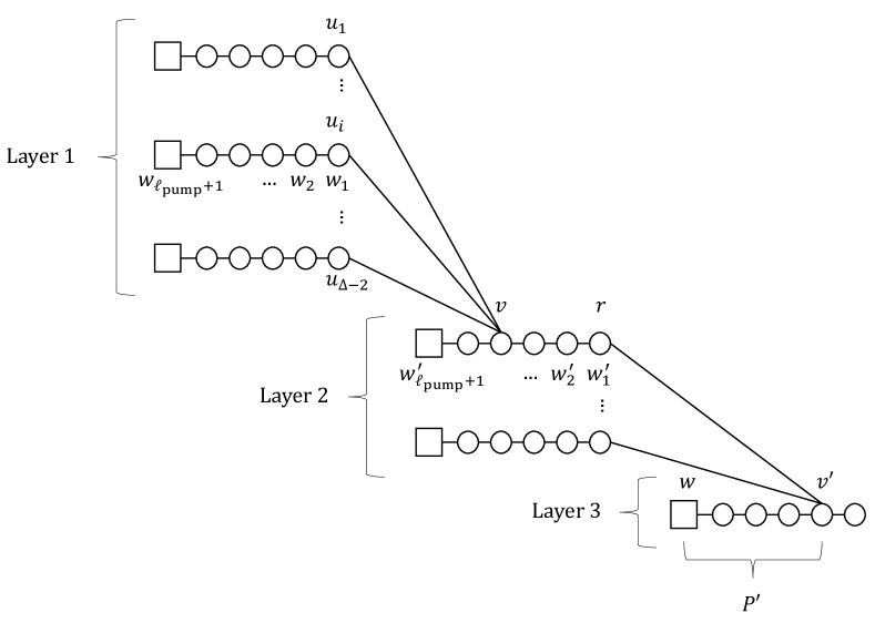
Figure 4: An illustration for the proof of Lemma 4.16.

For Lemma 4.17, note that if $\mathtt{a}$ appears more than once in the multiset $x$, then we still have $\mathtt{a}\in x\setminus\{\mathtt{a}\}$.

Lemma 4.17.

For any $\mathtt{a}\in x\in\mathcal{V}^{\ast}$, $\mathtt{a}^{\prime}\in x^{\prime}\in\mathcal{V}^{\ast}$, and $0\leq t\leq{\ell_{\operatorname{pump}}}-1$, we have $(x,\mathtt{b})\overset{k}{\leftrightarrow}(x^{\prime},\mathtt{b}^{\prime})$ for some $\mathtt{b}\in x\setminus\{\mathtt{a}\}$ and $\mathtt{b}^{\prime}\in x^{\prime}\setminus\{\mathtt{a}^{\prime}\}$ with $k=2{\ell_{\operatorname{pump}}}+4+t$.

Proof.

For any $\mathtt{a}\in x\in\mathcal{V}^{\ast}$, we can find a rooted tree $T_{x,\mathtt{a}}\in W_{2}^{\ast}$ such that the path $(v_{1}$, $v_{2}$, $\ldots$, $v_{{\ell_{\operatorname{pump}}}+1})$ of the layer-1 vertices in $T_{x,\mathtt{a}}$ where $v_{1}=r$ is the root of $T_{x,\mathtt{a}}$ satisfies the property that the half-edge labels of $v_{{\ell_{\operatorname{pump}}}+1}$ have been fixed to $x$ by $f$ where the half-edge label for $\{v_{{\ell_{\operatorname{pump}}}},v_{{\ell_{\operatorname{pump}}}+1}\}$ is in $x\setminus\{\mathtt{a}\}$.

Now, observe that for any choice of $(\Delta-2)({\ell_{\operatorname{pump}}}+1)$ rooted trees

$$\{T_{i,j}\}_{1\leq i\leq{\ell_{\operatorname{pump}}}+1,1\leq j\leq\Delta-2}$$

in $W_{2}^{\ast}$, there is a rooted tree $T^{\prime}\in W_{3}^{\ast}=Z_{f}(W_{2}^{\ast})$ formed by appending $T_{i,1}$, $T_{i,2}$, $\ldots$, $T_{i,\Delta-2}$ to $u_{i}$ in the path $(u_{1}$, $u_{2}$, $\ldots$, $u_{{\ell_{\operatorname{pump}}}+1})$ and fixing the half-edge labeling of $u_{{\ell_{\operatorname{pump}}}+1}$ by $f$. All vertices in $(u_{1},u_{2},\ldots,u_{{\ell_{\operatorname{pump}}}+1})$ are of layer-2.

We choose any $T^{\prime}\in W_{2}^{\ast}$ with $T_{i,j}=T_{x,\mathtt{a}}$ and $T_{i^{\prime},j^{\prime}}=T_{x^{\prime},\mathtt{a}^{\prime}}$ such that $i^{\prime}-i=t+1$. The possible range of $t$ is $[0,{\ell_{\operatorname{pump}}}-1]$. Consider any $T\in W_{L}^{\ast}$ that contains $T^{\prime}$ as its subtree, and consider any correct labeling of $T$. Then the path $P$ resulting from concatenating the path $(v_{{\ell_{\operatorname{pump}}}+1},v_{{\ell_{\operatorname{pump}}}},\ldots,v_{1})$ in $T_{x,\mathtt{a}}$, the path $(u_{i},u_{i+1},\ldots,u_{i^{\prime}})$, and the path $(v_{1}^{\prime},v_{2}^{\prime},\ldots,v_{{\ell_{\operatorname{pump}}}+1}^{\prime})$ in $T_{x^{\prime},\mathtt{a}^{\prime}}$ shows that $(x,\mathtt{b})\overset{k}{\leftrightarrow}(x^{\prime},\mathtt{b}^{\prime})$ for $k=({\ell_{\operatorname{pump}}}+1)+(t+2)+({\ell_{\operatorname{pump}}}+1)=2{\ell_{\operatorname{pump}}}+4+t$. See Fig. 5 for an illustration.

For the rest of the proof, we show that the desired rooted tree $T_{x,\mathtt{a}}\in W_{2}^{\ast}$ exists for any $\mathtt{a}\in x\in\mathcal{V}^{\ast}$. For any $x\in\mathcal{V}^{\ast}$, we can find a bipolar tree

$$H_{\ast}=(T_{1}^{l},T_{2}^{l},\ldots,T_{{\ell_{\operatorname{pump}}}}^{l},T_{\ast}^{m},T_{1}^{r},T_{2}^{r},\ldots,T_{{\ell_{\operatorname{pump}}}}^{r})\in Y_{1}^{\ast}=Y_{f}(W_{1}^{\ast})$$

such that the vertex configuration of the root $r^{m}$ of $T_{\ast}^{m}$ is fixed to be $x$ by the labeling function $f$. Then, for any $\mathtt{a}\in x$, at least one of the two rooted trees in $W_{2}^{\ast}=Z_{f}(W_{1}^{\ast})$ resulting from cutting $H_{\ast}$ satisfies the desired requirement. ∎

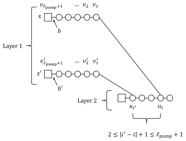
Figure 5: An illustration for the proof of Lemma 4.17.

In the subsequent discussion, the length of a path refers to the number of edges in a path. In particular, the length of a $k$-vertex path is $k-1$.

The following lemma is proved by iteratively applying Lemma 4.17 via intermediate vertex configurations $\tilde{x}\in\mathcal{V}^{\ast}$.

Lemma 4.18.

For any $\mathtt{a}\in x\in\mathcal{V}^{\ast}$ and $\mathtt{a}^{\prime}\in x^{\prime}\in\mathcal{V}^{\ast}$, we have $(x,\mathtt{b})\overset{k}{\leftrightarrow}(x^{\prime},\mathtt{b}^{\prime})$ for some $\mathtt{b}\in x\setminus\{\mathtt{a}\}$ and $\mathtt{b}^{\prime}\in x^{\prime}\setminus\{\mathtt{a}^{\prime}\}$ for all $k\geq 6{\ell_{\operatorname{pump}}}+10$.

Proof.

By applying Lemma 4.17 for three times, we infer that Lemma 4.17 also works for any path length $k-1=(k_{1}-1)+(k_{2}-1)+(k_{3}-1)$, where $k_{i}-1=2{\ell_{\operatorname{pump}}}+3+t_{i}$ for $0\leq t_{i}\leq{\ell_{\operatorname{pump}}}-1$.

Specifically, we first apply Lemma 4.17 to find a path realizing $(x,\mathtt{b})\overset{k_{1}}{\leftrightarrow}\tilde{x}$ for some $\tilde{x}\in\mathcal{V}^{\ast}$, and for some $\mathtt{b}\in x\setminus\{\mathtt{a}\}$. Let $\tilde{\mathtt{a}}\in\tilde{x}$ be the real half-edge label used in the last vertex of the path. We extend the length of this path by $k_{2}-1$ by attaching to it the path realizing $(\tilde{x},\tilde{\mathtt{b}})\overset{k_{2}}{\leftrightarrow}\tilde{x}$, for some $\tilde{\mathtt{b}}\in\tilde{x}\setminus\{\tilde{\mathtt{a}}\}$. Finally, let $\tilde{\mathtt{c}}\in\tilde{x}$ be the real half-edge label used in the last vertex of the current path. We extend the length of the current path by $k_{3}$ by attaching to it the path realizing $(\tilde{x},\tilde{\mathtt{d}})\overset{k_{3}}{\leftrightarrow}(x^{\prime},\mathtt{b}^{\prime})$, for some $\tilde{\mathtt{d}}\in\tilde{x}\setminus\{\tilde{\mathtt{x}}\}$, and for some $\mathtt{b}^{\prime}\in x^{\prime}\setminus\{\mathtt{a}^{\prime}\}$. The resulting path realizes $(x,\mathtt{b})\overset{k}{\leftrightarrow}(x^{\prime},\mathtt{b}^{\prime})$ for some $\mathtt{b}\in x\setminus\{\mathtt{a}\}$ and $\mathtt{b}^{\prime}\in x^{\prime}\setminus\{\mathtt{a}^{\prime}\}$.

Therefore, Lemma 4.17 also works with path length of the form $k-1=6{\ell_{\operatorname{pump}}}+9+t$, for any $t\in[0,3{\ell_{\operatorname{pump}}}-3]$.

Any $k-1\geq 6{\ell_{\operatorname{pump}}}+9$ can be written as $k-1=b(2{\ell_{\operatorname{pump}}}+3)+(6{\ell_{\operatorname{pump}}}+9+t)$, for some $t\in[0,3{\ell_{\operatorname{pump}}}-3]$ and some integer $b\geq 0$. Therefore, similar to the above, we can find a path showing $(x,\mathtt{b})\overset{k}{\leftrightarrow}(x^{\prime},\mathtt{b}^{\prime})$ by first applying Lemma 4.17 with path length $2{\ell_{\operatorname{pump}}}+3$ for $b$ times, and then applying the above variant of Lemma 4.17 to extend the path length by $6{\ell_{\operatorname{pump}}}+9+t$. ∎

We show that Lemmas 4.16 and 4.18 imply that $\mathcal{V}^{\prime}$ is $\ell$-full for some $\ell$.

Lemma 4.19 ($\mathcal{V}^{\prime}$ is $\ell$-full).

The set $\mathcal{V}^{\prime}$ is $\ell$-full for $\ell=10{\ell_{\operatorname{pump}}}+10$.

Proof.

We show that for any target path length $k-1\geq 10{\ell_{\operatorname{pump}}}+9$, and for any $\mathtt{a}\in x\in\mathcal{V}^{\ast}$ and $\mathtt{a}^{\prime}\in x^{\prime}\in\mathcal{V}^{\ast}$, we have $(x,\mathtt{a})\overset{k}{\leftrightarrow}(x^{\prime},\mathtt{a}^{\prime})$.

By Lemma 4.16, there exists a vertex configuration $\tilde{x}\in\mathcal{V}^{\ast}$ so that we can find a path $P$ realizing $(x,\mathtt{a})\overset{\ell_{1}}{\leftrightarrow}\tilde{x}$ for some path length $1\leq(\ell_{1}-1)\leq 2{\ell_{\operatorname{pump}}}$. Similarly, there exists a vertex configuration $\tilde{x}^{\prime}\in\mathcal{V}^{\ast}$ so that we can find a path $P^{\prime}$ realizing $(x^{\prime},\mathtt{a}^{\prime})\overset{\ell_{2}}{\leftrightarrow}\tilde{x}^{\prime}$ for some path length $1\leq(\ell_{2}-1)\leq 2{\ell_{\operatorname{pump}}}$.

Let $\tilde{\mathtt{a}}$ be the real half-edge label for $\tilde{x}$ in $P$, and let $\tilde{\mathtt{a}}^{\prime}$ be the real half-edge label for $\tilde{x}^{\prime}$ in $P^{\prime}$. We apply Lemma 4.18 to find a path $\tilde{P}$ realizing $(x,\mathtt{b})\overset{\tilde{\ell}}{\leftrightarrow}(x^{\prime},\mathtt{b}^{\prime})$ for some $\mathtt{b}\in\tilde{x}\setminus\{\tilde{\mathtt{a}}\}$ and $\mathtt{b}^{\prime}\in\tilde{x}^{\prime}\setminus\{\tilde{\mathtt{a}}^{\prime}\}$ with path length

$$\tilde{\ell}-1=(k-1)-(\ell_{1}-1)-(\ell_{2}-1)\geq 6{\ell_{\operatorname{pump}}}+9.$$

The path formed by concatenating $P_{1}$, $\tilde{P}$, and $P_{2}$ shows that $(x,\mathtt{a})\overset{k}{\leftrightarrow}(x^{\prime},\mathtt{a}^{\prime})$. ∎

A Feasible Labeling Function $f$ exists

We show that a feasible labeling function $f$ exists given that $\Pi$ can be solved in $\mathsf{LOCAL}(n^{o(1)})$ rounds. We will construct a labeling function $f$ in such a way each equivalence class in $\textsf{Class}_{1}(W^{\ast})$ contains only rooted trees that admit legal labeling. That is, for each $c\in\textsf{Class}_{1}(W^{\ast})$, the mapping $h$ associated with $c$ satisfies $h(X)=\textsf{YES}$ for some $X$.

We will consider a series of modifications in the construction

$$W\rightarrow X_{f}(W)\rightarrow Y_{f}(W)\rightarrow Z_{f}(W)$$

that do not alter the sets of equivalence classes in these sets, conditioning on the assumption that all trees that we have processed admit correct labelings. That is, whether $f$ is feasible is invariant of the modifications.

Applying the Pumping Lemma

Let $w>0$ be some target length for the pumping lemma. In the construction of $Y_{f}(W)$, when we process a bipolar tree

$$H=(T_{1}^{l},T_{2}^{l},\ldots,T_{{\ell_{\operatorname{pump}}}}^{l},T^{m},T_{1}^{r},T_{2}^{r},\ldots,T_{{\ell_{\operatorname{pump}}}}^{r}),$$

we apply Lemma 4.8 to the two subtrees $H^{l}=(T_{1}^{l},T_{2}^{l},\ldots,T_{{\ell_{\operatorname{pump}}}}^{l})$ and $H^{r}=(T_{1}^{r},T_{2}^{r},\ldots,T_{{\ell_{\operatorname{pump}}}}^{r})$ to obtain two new bipolar trees $H_{+}^{l}$ and $H_{+}^{r}$. The $s$-$t$ path in the new trees $H_{+}^{l}$ and $H_{+}^{r}$ contains $w+x$ vertices, for some $0\leq x<{\ell_{\operatorname{pump}}}$. The equivalence classes do not change, that is, $\textsf{Class}_{2}(H^{l})=\textsf{Class}_{2}(H_{+}^{l})$ and $\textsf{Class}_{2}(H^{r})=\textsf{Class}_{2}(H_{+}^{r})$.

We replace $H^{l}$ by $H_{+}^{l}$ and replace $H^{r}$ by $H_{+}^{r}$ in the bipolar tree $H$. Recall that the outcome of applying the labeling function $f$ to the root $r$ of the rooted tree $T_{{\ell_{\operatorname{pump}}}+1}$ depends only on

$$\textsf{Class}_{2}(H^{l}),\textsf{Class}_{1}(T_{1}^{m}),\textsf{Class}_{1}(T_{2}^{m}),\ldots,\textsf{Class}_{1}(T_{\Delta-2}^{m}),\textsf{Class}_{2}(H^{r}),$$

so applying the pumping lemma to $H^{l}$ and $H^{r}$ during the construction of $Y_{f}(W)$ does not alter $\textsf{Class}_{1}(T_{\ast}^{m})$ and $\textsf{Class}_{2}(H^{\ast})$ for the resulting bipolar tree $H^{\ast}$ and its middle rooted tree $T_{\ast}^{m}$, by Lemma 4.9.

Reusing Previous Trees

During the construction of the fixed point $W^{\ast}$, we remember all bipolar trees to which we have applied the feasible function $f$.

During the construction of $Y_{f}(W)$. Suppose that we are about to process a bipolar tree $H$, and there is already some other bipolar tree $\tilde{H}$ to which we have applied $f$ before so that $\textsf{Class}_{2}(H^{l})=\textsf{Class}_{2}(\tilde{H}^{l})$, $\textsf{Class}_{1}(T_{i}^{m})=\textsf{Class}_{1}(\tilde{T}_{i}^{m})$ for each $1\leq i\leq\Delta-2$, and $\textsf{Class}_{2}(H^{r})=\textsf{Class}_{2}(\tilde{H}^{r})$. Then we replace $H$ by $\tilde{H}$, and then we process $\tilde{H}$ instead.

By Lemma 4.9, this modification does not alter $\textsf{Class}_{1}(T_{\ast}^{m})$ and $\textsf{Class}_{2}(H^{\ast})$ for the resulting bipolar tree $H^{\ast}$.

Not Cutting Bipolar Trees

We consider the following different construction of $Z_{f}(W)$ from $Y_{f}(W)$. For each $H^{\ast}\in Y_{f}(W)$, we simply add two copies of $H^{\ast}$ to $Z_{f}(W)$, one of them has $r=s$ and the other one has $r=t$. That is, we do not cut the bipolar tree $H^{\ast}$, as in the original construction of $Z_{f}(W)$.

In general, this modification might alter $\textsf{Class}_{1}(Z_{f}(W))$. However, it is not hard to see that if all trees in $Y_{f}(W)$ already admit correct labelings, then $\textsf{Class}_{1}(Z_{f}(W))$ does not alter after the modification.

Specifically, let $T$ be a rooted tree in $Z_{f}(W)$ with the above modification. Then $T$ is identical to a bipolar tree $H^{\ast}=(T_{1},T_{2},\ldots,T_{k})\in Y_{f}(W)$, where there exists some $1<i<k$ such that the root $r_{i}$ of $T_{i}$ has its half-edge labels fixed by $f$. Suppose that the root of $T$ is the root $r_{1}$ of $T_{1}$. If we do not have the above modification, then the rooted tree $T^{\prime}$ added to $Z_{f}(W)$ corresponding to $T$ is $(T_{1},T_{2},\ldots,T_{i})$, where the root of $T^{\prime}$ is also $r_{1}$.

Given the assumption that all bipolar trees in $Y_{f}(W)$ admit correct labelings, it is not hard to see that $\textsf{Class}_{1}(T^{\prime})=\textsf{Class}_{1}(T)$. For any correct labeling $\mathcal{L}^{\prime}$ of $T^{\prime}$, we can extend the labeling to a correct labeling $\mathcal{L}$ of $T$ by labeling the remaining vertices according to any arbitrary correct labeling of $H^{\ast}$. This is possible because the labeling of $r_{i}$ has been fixed. For any correct labeling $\mathcal{L}$ of $T$, we can obtain a correct labeling $\mathcal{L}^{\prime}$ of $T^{\prime}$ by restricting $\mathcal{L}$ to $T^{\prime}$.

Simulating a $\mathsf{LOCAL}$ Algorithm

We will show that there is a labeling function $f$ that makes all the rooted trees in $W^{\ast}$ to admit correct solutions, where we apply the above three modifications in the construction of $W^{\ast}$. In view of the above discussion, such a function $f$ is feasible.

The construction of $W^{\ast}$ involves only a finite number $k$ of iterations of $Z_{f}$ applied to some previously constructed rooted trees. If we view the target length $w$ of the pumping lemma as a variable, then the size of a tree in $W^{\ast}$ can be upper bounded by $O(w^{k})$.

Suppose that we are given an arbitrary $n^{o(1)}$-round $\mathsf{LOCAL}$ algorithm $\mathcal{A}$ that solves $\Pi$. It is known [CP19, Cha20] that randomness does not help for LCL problems on bounded-degree trees with lound complexity $\Omega(\log n)$, so we assume that $\mathcal{A}$ is deterministic.

The runtime of $\mathcal{A}$ on a tree of size $O(w^{k})$ can be made to be at most $t=w/10$ if $w$ is chosen to be sufficiently large.

We pick the labeling function $f$ as follows. Whenever we encounter a new bipolar tree $H$ to which we need to apply $f$, we simulate $\mathcal{A}$ locally at the root $r^{m}$ of the middle rooted tree $T^{m}$ in $H$. Here we assume that the pumping lemma was applied before simulating $\mathcal{A}$. Moreover, when we do the simulation, we assume that the number of vertices is $n=O(w^{k})$.

To make the simulation possible, we just locally generate arbitrary distinct identifiers in the radius-$t$ neighborhood $S$ of $r^{m}$. This is possible because $t=w/10$ is so small that for any vertex $v$ in any tree $T$ constructed by recursively applying $Z_{f}$ for at most $k$ iterations, the radius-$(t+1)$ neighborhood of $v$ intersects at most one such $S$-set. Therefore, it is possible to complete the identifier assignment to the rest of the vertices in $T$ so that for any edge $\{u,v\}$, the set of identifiers seen by $u$ and $v$ are distinct in an execution of a $t$-round algorithm.

Thus, by the correctness of $\mathcal{A}$, the labeling of all edges $\{u,v\}$ are configurations in $\mathcal{E}$ and the labeling of all vertices $v$ are configurations in $\mathcal{V}$. Our choice of $f$ implies that all trees in $W^{\ast}$ admit correct labeling, and so $f$ is feasible. Combined with Lemma 4.19, we have proved that $\mathsf{LOCAL}(n^{o(1)})$ $\Rightarrow$ $\ell$-full.

Acknowledgements

We would like to thank Anton Bernshteyn, Endre Csóka, Mohsen Ghaffari, Jan Hladký, Steve Jackson, Alexander Kechris, Edward Krohne, Oleg Pikhurko, Brandon Seward, Jukka Suomela, and Yufan Zheng for insightful discussions.

YC was supported by Dr. Max Rössler, by the Walter Haefner Foundation, and by the ETH Zürich Foundation. JG was supported by Leverhulme Research Project Grant RPG-2018-424. CG and VR were supported by the European Research Council (ERC) under the European Unions Horizon 2020 research and innovation programme (grant agreement No. 853109). ZV was partially supported by the National Research, Development and Innovation Office – NKFIH, grants no. 113047, no. 129211 and FWF Grant M2779.

References

- [BBC+22] Alkida Balliu, Sebastian Brandt, Yi-Jun Chang, Dennis Olivetti, Jan Studenỳ, and Jukka Suomela. Efficient classification of local problems in regular trees. arXiv preprint arXiv:2202.08544, 2022.
- [BBE+20] Alkida Balliu, Sebastian Brandt, Yuval Efron, Juho Hirvonen, Yannic Maus, Dennis Olivetti, and Jukka Suomela. Classification of distributed binary labeling problems. In Hagit Attiya, editor, 34th International Symposium on Distributed Computing (DISC), volume 179 of Leibniz International Proceedings in Informatics (LIPIcs), pages 17:1–17:17, Dagstuhl, Germany, 2020. Schloss Dagstuhl–Leibniz-Zentrum für Informatik.
- [BBH+19] Alkida Balliu, Sebastian Brandt, Juho Hirvonen, Dennis Olivetti, Mikaël Rabie, and Jukka Suomela. Lower bounds for maximal matchings and maximal independent sets. In Proceedings of the IEEE 60th Annual Symposium on Foundations of Computer Science (FOCS), pages 481–497, 2019.
- [BBKO21] Alkida Balliu, Sebastian Brandt, Fabian Kuhn, and Dennis Olivetti. Improved distributed lower bounds for MIS and bounded (out-)degree dominating sets in trees. In Proceedings of the 2021 ACM Symposium on Principles of Distributed Computing (PODC), 2021.
- [BBKO22] Alkida Balliu, Sebastian Brandt, Fabian Kuhn, and Dennis Olivetti. Distributed -coloring plays hide-and-seek. In 54th ACM Symposium on Theory of Computing (STOC), 2022.
- [BBO20] Alkida Balliu, Sebastian Brandt, and Dennis Olivetti. Distributed lower bounds for ruling sets. In 61st IEEE Annual Symposium on Foundations of Computer Science, FOCS 2020, Durham, NC, USA, November 16-19, 2020, pages 365–376, 2020.
- [BBO+21] Alkida Balliu, Sebastian Brandt, Dennis Olivetti, Jan Studený, Jukka Suomela, and Aleksandr Tereshchenko. Locally checkable problems in rooted trees. In Proceedings of the 2021 ACM Symposium on Principles of Distributed Computing, 2021.
- [BBOS20] Alkida Balliu, Sebastian Brandt, Dennis Olivetti, and Jukka Suomela. Almost global problems in the local model. Distributed Computing, pages 1–23, 2020.
- [BCG+21a] Sebastian Brandt, Yi-Jun Chang, Jan Grebík, Christoph Grunau, Vaclav Rozhoň, and Zoltán Vidnyánszky. Complexity classes of local problems on trees from the perspectives of distributed algorithms, finitary factors, and descriptive combinatorics. in preparation, 2021.
- [BCG+21b] Sebastian Brandt, Yi-Jun Chang, Jan Grebík, Christoph Grunau, Vaclav Rozhoň, and Zoltán Vidnyánszky. Local problems on trees from the perspectives of distributed algorithms, finitary factors, and descriptive combinatorics. arXiv preprint arXiv:2106.02066, 2021. A short version of the paper was presented at the 13th Innovations in Theoretical Computer Science conference (ITCS 2022).
- [BCG+21c] Sebastian Brandt, Yi-Jun Chang, Jan Grebík, Christoph Grunau, Václav Rozhoň, and Zoltán Vidnyánszky. On homomorphism graphs, 2021.
- [BEPS16] Leonid Barenboim, Michael Elkin, Seth Pettie, and Johannes Schneider. The locality of distributed symmetry breaking. Journal of the ACM, 63(3):20, 2016.
- [Ber] Anton Bernshteyn. Work in progress.
- [Ber20a] Anton Bernshteyn. Distributed algorithms, the Lovász Local Lemma, and descriptive combinatorics. arXiv preprint arXiv:2004.04905, 2020.
- [Ber20b] Anton Bernshteyn. A fast distributed algorithm for (+1)-edge-coloring. preprint, 2020.
- [Ber21] Anton Bernshteyn. Probabilistic constructions in continuous combinatorics and a bridge to distributed algorithms. arXiv preprint arXiv:2102.08797, 2021.
- [BFH+16] Sebastian Brandt, Orr Fischer, Juho Hirvonen, Barbara Keller, Tuomo Lempiäinen, Joel Rybicki, Jukka Suomela, and Jara Uitto. A lower bound for the distributed Lovász local lemma. In Proc. 48th ACM Symp. on Theory of Computing (STOC), pages 479–488, 2016.
- [BGH19] Ágnes Backhausz, Balázs Gerencsér, and Viktor Harangi. Entropy inequalities for factors of IID. Groups Geom. Dyn., 13(2):389–414, 2019.
- [BGR20] Sebastian Brandt, Christoph Grunau, and Václav Rozhoň. Generalizing the sharp threshold phenomenon for the distributed complexity of the lovász local lemma. In Proceedings of the 39th Symposium on Principles of Distributed Computing, pages 329–338, 2020.
- [BHK+17] Sebastian Brandt, Juho Hirvonen, Janne H. Korhonen, Tuomo Lempiäinen, Patric R.J. Östergård, Christopher Purcell, Joel Rybicki, Jukka Suomela, and Przemysław Uznański. LCL problems on grids. In Proceedings of the ACM Symposium on Principles of Distributed Computing (PODC), page 101–110, New York, NY, USA, 2017. Association for Computing Machinery.
- [BHK+18] Alkida Balliu, Juho Hirvonen, Janne H Korhonen, Tuomo Lempiäinen, Dennis Olivetti, and Jukka Suomela. New classes of distributed time complexity. In Proceedings of the 50th Annual ACM SIGACT Symposium on Theory of Computing, pages 1307–1318, 2018.
- [BHOS19] Alkida Balliu, Juho Hirvonen, Dennis Olivetti, and Jukka Suomela. Hardness of minimal symmetry breaking in distributed computing. In Proceedings of the 2019 ACM Symposium on Principles of Distributed Computing, pages 369–378, 2019.
- [BO20] Sebastian Brandt and Dennis Olivetti. Truly tight-in- bounds for bipartite maximal matching and variants. In Proceedings of the 39th Symposium on Principles of Distributed Computing, PODC ’20, page 69–78, New York, NY, USA, 2020. Association for Computing Machinery.
- [Bow10a] Lewis Bowen. The ergodic theory of free group actions: entropy and the f -invariant. Groups Geom. Dyn., 4(3):419–432, 2010.
- [Bow10b] Lewis Bowen. A measure-conjugacy invariant for free group actions. Ann. of Math., 171(2):1387–1400, 2010.
- [Bra19] Sebastian Brandt. An automatic speedup theorem for distributed problems. In Proceedings of the 2019 ACM Symposium on Principles of Distributed Computing, PODC 2019, Toronto, ON, Canada, July 29 - August 2, 2019, pages 379–388, 2019.
- [BSV15] Ágnes Backhausz, Balázs Szegedy, and Bálint Virág. Ramanujan graphings and correlation decay in local algorithms. Random Structures Algorithms, 47(3):424–435, 2015.
- [CGA+16] Endre Csóka, Łukas Grabowski, Máthé András, Oleg Pikhurko, and Konstantin Tyros. Borel version of the local lemma. arXiv preprint arXiv:1605.04877, 2016.
- [CGM+17] Endre Csóka, Łukasz Grabowski, András Máthé, Oleg Pikhurko, and Konstantinos Tyros. Borel version of the Local Lemma. arXiv:1605.04877, 2017.
- [Cha20] Yi-Jun Chang. The Complexity Landscape of Distributed Locally Checkable Problems on Trees. In Hagit Attiya, editor, 34th International Symposium on Distributed Computing (DISC 2020), volume 179 of Leibniz International Proceedings in Informatics (LIPIcs), pages 18:1–18:17, Dagstuhl, Germany, 2020. Schloss Dagstuhl–Leibniz-Zentrum für Informatik.
- [CHL+20] Yi-Jun Chang, Qizheng He, Wenzheng Li, Seth Pettie, and Jara Uitto. Distributed edge coloring and a special case of the constructive Lovász local lemma. ACM Trans. Algorithms, 16(1):8:1–8:51, 2020.
- [CJM+20] Clinton T. Conley, Steve Jackson, Andrew S. Marks, Brandon Seward, and Robin Tucker-Drob. Borel asymptotic dimension and hyperfinite equivalence relations. arXiv:2009.06721, 2020.
- [CKP19] Yi-Jun Chang, Tsvi Kopelowitz, and Seth Pettie. An exponential separation between randomized and deterministic complexity in the local model. SIAM Journal on Computing, 48(1):122–143, 2019.
- [CM16] Clinton T. Conley and Benjamin D. Miller. A bound on measurable chromatic numbers of locally finite Borel graphs. Math. Res. Lett., 23(6):1633–1644, 2016.
- [CM17] Clinton T. Conley and Benjamin D. Miller. Measure reducibility of countable Borel equivalence relations. Ann. of Math. (2), 185(2):347–402, 2017.
- [CMTD16] Clinton T Conley, Andrew S Marks, and Robin D Tucker-Drob. Brooks’theorem for measurable colorings. In Forum of Mathematics, Sigma, volume 4. Cambridge University Press, 2016.
- [CP19] Yi-Jun Chang and Seth Pettie. A time hierarchy theorem for the local model. SIAM Journal on Computing, 48(1):33–69, 2019.
- [CSS20] Yi-Jun Chang, Jan Studený, and Jukka Suomela. Distributed graph problems through an automata-theoretic lens. arXiv:2002.07659, 2020.
- [CV86] Richard Cole and Uzi Vishkin. Deterministic coin tossing with applications to optimal parallel list ranking. Information and Control, 70(1):32–53, 1986.
- [DF92] Randall Dougherty and Matthew Foreman. Banach-Tarski paradox using pieces with the property of Baire. Proc. Nat. Acad. Sci. U.S.A., 89(22):10726–10728, 1992.
- [DJK94] Randall Dougherty, Steve Jackson, and Alexander S. Kechris. The structure of hyperfinite Borel equivalence relations. Trans. Amer. Math. Soc., 341(1):193–225, 1994.
- [Ele18] Gábor Elek. Qualitative graph limit theory. cantor dynamical systems and constant-time distributed algorithms. arXiv preprint arXiv:1812.07511, 2018.
- [Gab00] Damien Gaboriau. Coût des relations d’équivalence et des groupes. Invent. Math., 139(1):41–98, 2000.
- [Gao08] Su Gao. Invariant descriptive set theory. Chapman and Hall/CRC, 2008.
- [GHS14] Mika Göös, Juho Hirvonen, and Jukka Suomela. Linear-in- lower bounds in the LOCAL model. In Proc. 33rd ACM Symp. on Principles of Distributed Computing (PODC), pages 86–95, 2014.
- [GJ15] Su Gao and Steve Jackson. Countable abelian group actions and hyperfinite equivalence relations. Inventiones Math., 201(1):309–383, 2015.
- [GJKS] S. Gao, S. Jackson, E. Krohne, and B. Seward. Borel combinatorics of countable group actions. in prep.
- [GJKS15] Su Gao, Steve Jackson, Edward Krohne, and Brandon Seward. Forcing constructions and countable borel equivalence relations. arXiv:1503.07822, 2015.
- [GJKS18] Su Gao, Steve Jackson, Edward Krohne, and Brandon Seward. Continuous combinatorics of abelian group actions., 2018.
- [GJS09] S. Gao, S. Jackson, and B. Seward. A coloring property for countable groups. Mathematical Proceedings of the Cambridge Philosophical Society, 147(3):579–592, 2009.
- [GKM17] Mohsen Ghaffari, Fabian Kuhn, and Yannic Maus. On the complexity of local distributed graph problems. In Proc. 49th ACM Symp. on Theory of Computing (STOC), pages 784–797, 2017.
- [GMP17] Łukasz Grabowski, András Máthé, and Oleg Pikhurko. Measurable circle squaring. Ann. of Math. (2), 185(2):671–710, 2017.
- [GR21a] Jan Grebík and Václav Rozhoň. Classification of local problems on paths from the perspective of descriptive combinatorics. arXiv preprint arXiv:2103.14112, 2021.
- [GR21b] Jan Grebík and Václav Rozhoň. Local problems on grids from the perspective of distributed algorithms, finitary factors, and descriptive combinatorics. arXiv preprint arXiv:2103.08394, 2021.
- [GRB22] Christoph Grunau, Václav Rozhoň, and Sebastian Brandt. The landscape of distributed complexities on trees and beyond. ArXiv, abs/2202.04724, 2022.
- [HK96] Greg Hjorth and Alexander S. Kechris. Borel equivalence relations and classifications of countable models. Annals of pure and applied logic, 82(3):221–272, 1996.
- [HSW17] Alexander E. Holroyd, Oded Schramm, and David B. Wilson. Finitary coloring. Ann. Probab., 45(5):2867–2898, 2017.
- [JKL02] Steve Jackson, Alexander S. Kechris, and Alain Louveau. Countable Borel equivalence relations. J. Math. Logic, 2(01):1–80, 2002.
- [Kec95] Alexander S. Kechris. Classical descriptive set theory, volume 156 of Graduate Texts in Mathematics. Springer-Verlag, New York, 1995.
-
[KM20]
Alexander S. Kechris and Andrew S. Marks.
Descriptive graph combinatorics.
http://www.math.caltech.edu/~kechris/papers/combinatorics20book.pdf, 2020. - [KMW16] Fabian Kuhn, Thomas Moscibroda, and Roger Wattenhofer. Local computation: Lower and upper bounds. Journal of the ACM, 63(2), 2016.
- [KST99] Alexander S. Kechris, Sławomir Solecki, and Stevo Todorčević. Borel chromatic numbers. Adv. Math., 141(1):1–44, 1999.
- [Lac90] Miklós Laczkovich. Equidecomposability and discrepancy; a solution of Tarski’s circle-squaring problem. J. Reine Angew. Math., 404:77–117, 1990.
- [Lin92] Nati Linial. Locality in distributed graph algorithms. SIAM Journal on Computing, 21(1):193–201, 1992.
- [LN11] Russell Lyons and Fedor Nazarov. Perfect matchings as iid factors on non-amenable groups. European Journal of Combinatorics, 32(7):1115–1125, 2011.
- [Mar16] Andrew S. Marks. A determinacy approach to Borel combinatorics. J. Amer. Math. Soc., 29(2):579–600, 2016.
- [MNP22] András Máthé, Jonathan A. Noel, and Oleg Pikhurko. Circle squaring with pieces of small boundary and low borel complexity. arXiv:2202.01412, 2022.
- [MR89] Gary L. Miller and John H. Reif. Parallel tree contraction–Part I: fundamentals. Advances in Computing Research, 5:47–72, 1989.
- [MU16] Andrew Marks and Spencer Unger. Baire measurable paradoxical decompositions via matchings. Adv. Math., 289:397–410, 2016.
- [MU17] Andrew S. Marks and Spencer T. Unger. Borel circle squaring. Ann. of Math. (2), 186(2):581–605, 2017.
- [NS95] Moni Naor and Larry Stockmeyer. What can be computed locally? SIAM Journal on Computing, 24(6):1259–1277, 1995.
- [Pik21] Oleg Pikhurko. Borel combinatorics of locally finite graphs. arXiv preprint arXiv:2009.09113, 2021.
- [RG20] Václav Rozhoň and Mohsen Ghaffari. Polylogarithmic-time deterministic network decomposition and distributed derandomization. In Proc. Symposium on Theory of Computation (STOC), 2020.
- [STD16] B. Seward and R. Tucker-Drob. Borel structurability on the 2-shift of a countable group. Annals of Pure and Applied Logic, 167(1):1–21, 2016.