Self-supervised Learning for Sonar Image Classification

Abstract

Self-supervised learning has proved to be a powerful approach to learn image representations without the need of large labeled datasets. For underwater robotics, it is of great interest to design computer vision algorithms to improve perception capabilities such as sonar image classification. Due to the confidential nature of sonar imaging and the difficulty to interpret sonar images, it is challenging to create public large labeled sonar datasets to train supervised learning algorithms. In this work, we investigate the potential of three self-supervised learning methods (RotNet, Denoising Autoencoders, and Jigsaw) to learn high-quality sonar image representation without the need of human labels. We present pre-training and transfer learning results on real-life sonar image datasets. Our results indicate that self-supervised pre-training yields classification performance comparable to supervised pre-training in a few-shot transfer learning setup across all three methods. Code and self-supervised pre-trained models are be available at agrija9/ssl-sonar-images.

1 Introduction

Machine perception in autonomous underwater systems is considered an exceptionally challenging task due to the unpredictability of marine environments. Factors such as poor lighting conditions, sediments, and turbidity impact the visual-based sensing of underwater systems and can result in failure of critical localization and exploration missions. Acoustic-based imaging provides an alternative sensing modality that is unimpeded by visibility conditions and could operate in turbid waters or complete darkness. The main challenges faced however with acoustic sensors such as imaging sonars are low signal-to-noise ratios and other disturbances such as acoustic shadows, multipath interference [32] and crosstalk noise [35].

In recent years, deep neural network (DNN) architectures have become more popular in underwater applications like image enhancement [20, 35], sonar object classification [38, 40, 42], and sonar-camera image translation [37, 18]. For underwater sonar data specifically, the progress of deep learning research has been hindered due to the lack of publicly available data, which could be contributed to the costly operations needed to collect sonar data as well as confidentiality issues regarding military applications. To compensate for small datasets and lack of annotated data, self-supervised learning (SSL) [19, 17, 27] has become an effective technique that attempts to learn data representations by using data itself as a supervision signal.

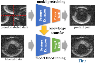
Figure 1: We propose to expand the capabilities of self-supervised learning to the sonar image domain with applications to underwater robotics. Our conceptual idea of self-supervision on grayscale sonar images follows successful established approaches where we pretrain models on large unlabeled sonar datasets and evaluate them using transfer learning on smaller labeled sonar datasets.

The main contribution of this work is the evaluation of relevant SSL algorithms for sonar image data with applications to object classification. In Fig. 1 we illustrate our proposed conceptual approach. We have studied three SSL algorithms (RotNet [6], Denoising Autoencoders [41], and Jigsaw [30]) and compared them to their supervised learning (SL) counterpart. The SSL algorithms were trained on an experimental real-life sonar dataset, where the learned representation quality was evaluated using a low-shot transfer learning setup on another real-life test sonar dataset. Our findings indicate that all SSL models can reach a similar performance to that of their supervised counterparts. This holds even when using a completely unlabeled on-the-wild sonar dataset. We also note that unlike color image datasets, SSL does not by itself outperform supervised learning.

These results indicate that SSL has the potential to replace the need for labeled sonar data without compromising task performance and reducing the time and costs of data labeling.

2 Related Work

Self-supervised learning (SSL) is a learning paradigm that presents itself as a more scalable approach to pretrain models for transfer learning with less human labeled data [2, 3, 9, 11]. SSL can be understood as a two-step approach: a) learning data representation from solving a proxy or pretext task using automatically generated pseudo-labels from raw-unlabeled data, followed by b) fine-tuning of the learned features on the actual downstream task, i.e. task of interest such as classification, segmentation or detection tasks, with few manually labeled data by using transfer learning.

SSL has been mainly used in color images demonstrating not only the capability to reach same performance than pure supervised learning methods with much less labeled data for many tasks, but even surpassing their performance in some cases [19]. Pretext tasks that have shown promising results in learning strong latent representations in color images are a) generation-based methods, such as image colorization [44, 45, 22], super-resolution [23], image denoising [41], in-painting [31, 16] and video prediction [33], b) spatial context methods, such as solving the jigsaw puzzle [30, 36] and recognizing rotations [6], and c) temporal context methods, such as recognizing the order of the frame sequence [29, 24]. A detailed description of the chosen pretext tasks widely used for color images that we believe can be applied for sonar images are given in section 4.

Although self-supervised learning has been demonstrated to improve performance in color images for many downstream tasks, it has not yet been applied to sonar images to the best of our knowledge. However, a few studies on supervised pre-training for transfer learning have been carried out showing great potential for the use of SSL with sonar images [39, 38, 40]. For example, [39] made a study on the effect of the training set size by using transfer learning in sonar image for object recognition, some of the proposed architectures required only 50 samples per class to achieve 90% accuracy indicating that deep convolutional neural network (deep CNN) models can generalize well to other data distributions even with few samples per class.

3 Sonar Datasets

One of the most important things to build robust and reliable deep learning vision models is to test them across different datasets in order to see how they perform against varying data distributions. In this section, we describe the sonar datasets we used to train and evaluate our self-supervised learning algorithms. In particular, we used the Marine Debris Watertank dataset in the pre-training phase and the Marine Debris Turntable dataset to evaluate the quality of the learned features during pre-training. Both datasets were introduced in [40].

Marine Debris Watertank. This dataset contains a total of 2627 forward-looking sonar (FLS) images grouped across 11 classes. This dataset was collected with an ARIS Explorer 3000 FLS at a frequency of 3.0 MHz. The dataset was split into three sets: 70% for training, 15% for validation and 15% for testing. We used this dataset exclusively to pretrain the three self-supervised models proposed in this paper. Fig. 2 shows objects sampled from this dataset.

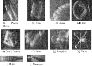
Figure 2: Samples of sonar images from the Watertank dataset.

Marine Debris Turntable. This dataset contains a total of 2471 sonar images grouped across 12 classes. This dataset was also collected using an ARIS Explorer 3000 FLS at the highest frequency. Each object in this dataset was placed underwater on a rotating table so that the images for each object were captured at different angles along the z-axis. As mentioned in [40], generating multiple views from objects can help learn better image features since sonar image properties changes with the view angle (e.g. reflections, pose, and sensor noise). There is an intersection between both datasets since they have some objects in common (approximately 50% of the objects). This means that they are not completely independent. Fig. 3 shows samples of the objects on top of the rotating platform.

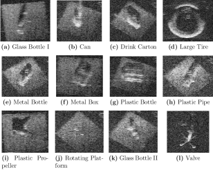
Figure 3: Samples of sonar images from the Turntable dataset.

4 Sonar Image Classification

In this section, we present pre-training experiments of three self-supervised models: RotNet [6], Denoising Autoencoders (DAEs) [41] and Jigsaw Puzzle [30]. Furthermore, we evaluate their generalization capacities in a few-shot transfer learning setup for sonar image classification. We used the Watertank dataset for pre-training and the Turntable dataset for transfer learning. The research question we address here is whether self-supervised pre-training provides high-quality image features that can compete (or be better) when compared to image features obtained via supervised pre-training. We have chosen these methods due to their success in applications such as image rotations [5, 12], image denoising [25, 34, 43], and jigsaw puzzle solving [8, 26, 28].

4.1 RotNet - Learning Sonar Image Representations by Predicting Rotations

RotNet [6] learns representations by predicting rotation angles applied to input images as opposed to predicting actual object labels. As discussed in [6], replacing human labels with synthetically generated rotation labels can be an alternative to learn high-quality representations without the need for costly and time-consuming human annotations. Refer to Appendix B for a detailed description of the baseline models we implemented to train RotNet.

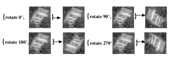
Figure 4: Applying rotations to sonar images to generate various synthetic perspectives from the same object.

4.1.1 Pre-processing and Hyper-parameter Tuning

We followed the training procedure from [6] by applying a total of four rotation angles $\{0^{o},90^{o},180^{o},270^{o}\}$ to the sonar images from the Watertank dataset, see Fig. 4. Each angle has an integer label associated to it, hence, each image sample has the form $\chi_{rotnet}=$ (image$\_0^{o}$, 1), (image$\_90^{o}$, 2), (image$\_180^{o}$, 3), (image$\_270^{o}$, 4).

Similar to the experimental procedure from [40], we tuned a hyper-parameter w that corresponds to the number of filters or neurons for each one of the baseline models described previously. These models were originally designed and optimized to perform on standard color images, so it is necessary to fine-tune them for grayscale sonar images. In our case, each architecture has been modified into its shallowest variation, reducing the width parameter w in each case. We find that 128 filters as a maximum threshold across all architectures achieve good task performance (as opposed to the 1024 original filters). We found, in agreement with [40], that the best performing w parameters are the ones reported in Tab. 1.

Architecture	Selected width w	Use of w in architecture
ResNet20	32	w is set as starting number of filters, it duplicates itself after each residual stack (w = 2w).
MobileNet	32	Base filters are set to w, increasing first by a factor of four (w = 4w), then duplicating themselves.
DenseNet121	16	w is used as the number of filters for each convolutional layer inside each dense block
SqueezeNet	32	Base squeeze filters are set to w, and expansion filters are set to 2w, duplicating itself after each fire module stack.
MiniXception	16	Stem widths are set to [w/2, w], and block widths to [w, 2w, 4w, 8w].

Table 1: Selected w width parameter based on best performance for all models. Table and values obtained from [40].

4.1.2 Self-Supervised Training on Watertank Dataset

We trained our models on an NVIDIA Tesla V100 GPU (8GB of memory) using Keras and Tensorflow 2. Each architecture was trained with the Adam optimizer [21], a learning rate $\beta=0.001$ and a total of 200 epochs (except MobileNet with 220 epochs). All models were trained with sonar images of size $96\times 96$. During training, we applied real-time random shifts $s_{w}$, $s_{h}$ to each image (horizontal and vertical), these shifts were sampled from a uniform distribution $s_{w}\sim\textit{U}(0,0.1\textit{w})$ and $s_{h}\sim\textit{U}(0,0.1\textit{h})$. Additionally, we applied random up-down and left-right flips with 50% probability each one. We observed that normalizing the dataset by dividing pixel values by 255 causes unstable training, due to this, we restored to the mean subtraction normalization as performed in [40]. The pixel mean value of the training set is $\mu_{\text{pixel}}=84.5$ and normalization on each image is given by $x_{\text{normalized}}=x-\mu_{\text{pixel}}$.

Tab. 2 summarizes our training results on the Watertank dataset. The best performing model is ResNet20 followed by MiniXception. We provide self-supervised classification accuracies (for rotation labels) and supervised classification accuracies (for actual class labels). In this case, we have been able to apply standard supervised classification since we have the class labels from the Watertank objects.

Baseline Model	Rotation Accuracy (SSL)	True label Accuracy (SL)
ResNet20	97.22%	96.46%
MobileNet	94.43%	98.23%
DenseNet121	95.38%	96.46%
SqueezeNet	95%	97.47%
Minixception	96.14%	96.71%
Linear SVM	76.40%	96.70%

Table 2: RotNet pre-training classification results on the test set of the Watertank dataset. Results are shown for all baseline CNN architectures.

4.1.3 Transfer Learning on Turntable Dataset

In order to evaluate the quality of the features learned by the models from the previous section, we performed transfer learning on the Turntable dataset. In this setup, we first subsampled the training set of the Turntable dataset to have samples-per-class (spc) $\in[10,20,30,40,50,80,110,140,170,200]$ (to resemble a few-shot learning scheme). Thereafter, we generated embeddings of each subsampled training set using the pretrained models from above (we selected three hidden layers in each case close to the output, usually Flatten or last ReLU/Batch Normalization layers). Lastly, we used the embeddings to train a support vector machine classifier (SVM) with parameter $C=1.0$ (regularization parameter) for each spc (a total of 10 times to obtain a mean accuracy and standard deviation). Note that the SVM was not tuned though a cross-validation approach as the goal is to show the benefit SSL regardless of the performance of the model used for transfer learning.

We decided to use the linear SVM classifier as a first test of linear separability without having to perform further fine-tuning for transfer learning. We quantified sample complexity by recording classification accuracy on the test set of the Turntable dataset for each pretrained model, spc and hidden layer.

Our transfer learning results are presented in Fig. 5(a-e). We show the accuracy curves for each model as the samples per each class in the Turntable dataset increase. The green lines correspond to supervised pre-training and the red lines correspond to self-supervised pre-training. We observe that the red (SSL) lines have a similar performance compared to the green lines (SL) in terms of classification accuracy. Furthermore, there are even cases where self-supervised pre-training is better than supervised pre-training (e.g. MobileNet with conv-pw-11-relu layer).

These results are an important first indicator that self-supervised pre-training can be a replacement for supervised pre-training for sonar image classification tasks, thus removing the necessity of labeling large sonar datasets manually. The best self-supervised performing model (based on accuracy) corresponds to ResNet20, activation-17 layer with an accuracy of $96.62\pm 0.562\%$, which is less than 1% difference compared to the best supervised performing model ResNet20, activation-18 layer with $97.27\textpm 0.60\%$. Refer to Tab. 6 in Appendix C for a detailed summary of all RotNet transfer learning evaluations.

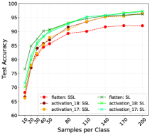
(a) ResNet20

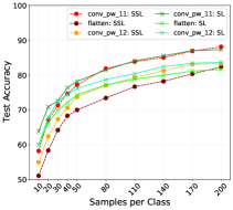
(b) MobileNet

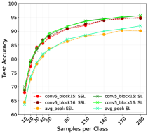
(c) DenseNet121

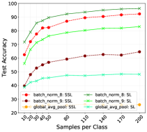
(d) SqueezeNet

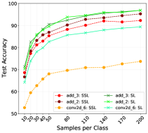
(e) MiniXception

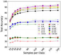
(f) Denoising Autoencoder

Figure 5: Transfer learning results on the Turntable dataset for models pretrained on the Watertank dataset. Multiple selected hidden layers and number of samples per class are presented. Red lines: self-supervised pre-training, green lines: supervised pre-training.

4.2 Denoising Autoencoder - Learning Sonar Image Representations by Denoising Corrupted Inputs

The Denoising Autoencoder (DAE) [41] applies Gaussian noise to input images and attempts to reconstruct the original uncorrupted inputs in an encoding-decoding manner. In the case of sonar images, this model is a good candidate to learn image representations while filtering noise out; this is of particular interest since most real-life sonar imaging scenarios consist of noisy images. Refer to Appendix D for a detailed description of the DAE architecture. In the following sections, we present pre-training and transfer learning experiments using the DAE algorithm.

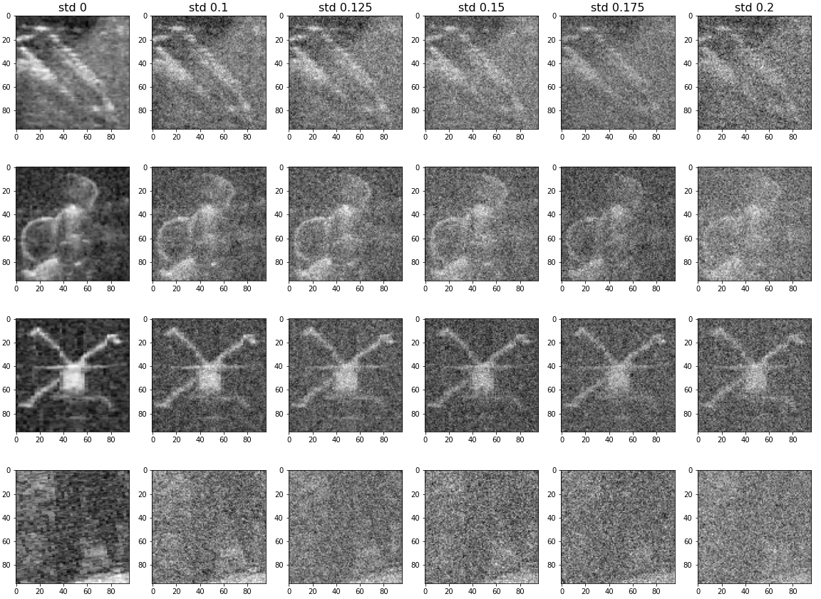
Figure 6: Different Gaussian noise standard deviation $\sigma$ applied to sonar images.

4.2.1 Self-Supervised Training on Watertank Dataset

We trained the DAE with the standard Mean Squared Error (MSE) and Mean Average Error (MAE) loss metrics. Similar to RotNet, we implemented Adam optimizer, trained for 200 epochs, used batch sizes of 128, and a learning rate $\beta=0.001$. Furthermore, we varied the code size (dimension of the intermediate layer) in the ranges $c\in[4,8,16,32,64,128]$, with each value $c$ producing a different autoencoder model. This is a main parameter of the architecture as it can have an important impact on reconstruction performance. Gaussian noise was applied to each input image using Keras built-in Gaussian Noise Layer. The main parameter of this noise layer is the standard deviation ($\sigma$) of the noise distribution as it controls the level of corruption applied to an image. During training, we have varied this value to $\sigma\in[0.100,0.125,0.150,0.175,0.200]$ to evaluate pre-training performance in the presence of different levels of noise (see Fig. 6). In Tab. 3 we show the reconstruction results on the test set of the Watertank dataset for varying code sizes $c$ and $\sigma$. From these experiments, we observed that high code sizes ($c=64,128$) and lower $\sigma$ (due to less corruption) yield better reconstructions.

		Noise Standard Deviation $\mathbf{\sigma}$
Code Size	Metric	$\mathbf{0.125}$	$\mathbf{0.150}$	$\mathbf{0.175}$	$\mathbf{0.200}$
4	MSE	0.04	0.05	0.05	0.03
	MAE	0.17	0.19	0.20	0.13
8	MSE	0.05	0.04	0.03	0.05
	MAE	0.19	0.18	0.13	0.19
16	MSE	0.04	0.05	0.07	0.06
	MAE	0.17	0.20	0.24	0.21
32	MSE	0.03	0.05	0.04	0.04
	MAE	0.15	0.20	0.19	0.18
64	MSE	0.03	0.03	0.03	0.04
	MAE	0.15	0.16	0.16	0.18
128	MSE	0.02	0.03	0.03	0.04
	MAE	0.12	0.16	0.14	0.17

Table 3: DAE pre-training reconstruction results on the test set of the Watertank dataset. Results are shown for varying code sizes and standard deviations.

4.2.2 Transfer Learning on Turntable Dataset

Following a similar procedure as with RotNet, we have generated image embeddings with the pretrained DAE models and trained an SVM classifier by sub-sampling the training set of the Turntable dataset. In this case, we only used the encoder as a feature extractor for embedding generation, i.e. the encoder maps the input images of size $96\times 96$ into a $1\times c$ vector embedding for each code size $c$.

In Fig. 5(f), we show the transfer learning results for one DAE model ($\sigma=0.1$) and an Auto Encoder (AE) (no denoising) and compare their performances across multiple code sizes $c$. We observed that there is a considerable gap in accuracies between DAE and AE for code size 4 (red lines). However, as we increased the code size, accuracies increase and the gap between both models decreases, indicating that higher dimensions can encode the original images more efficiently. For code size 128 for example, DAE performed better than AE, this indicates that adding noise as a form of random data augmentation can improve model performance. In this case, the best performing DAE (code size 128, $\sigma=0.150$) obtained an accuracy of $94.49\pm 0.62\%$, more than 2% over the best performing AE with $92.21\pm 0.59\%$. For a complete summary of our transfer learning experiments, refer to Tab. 7 in Appendix E, which contains results for the best performing code sizes and all standard deviations.

4.3 Jigsaw Puzzle - Learning Sonar Image Representations by Solving Jigsaw Puzzles

The Jigsaw algorithm [30] generates shuffled patches from input images as a form of self-supervision. First, an image is split into a $n\times n$ grid, yielding a total of $n^{2}$ image patches. Thereafter, the patches are shuffled based on predefined permutation sets. Although there are $n!$ possible permutation sets, this can be narrowed down as desired (based on memory limitations). The goal of this algorithm is to classify which permutation set has been applied to a given input image. Refer to Appendix F for a description of the Jigsaw architecture implemented. In the following sections, we describe technical aspects related to data generation, pre-training, and transfer learning evaluations of Jigsaw.

4.3.1 Puzzle Data Generation

In order to generate jigsaw puzzles from the Watertank sonar dataset, first, we split them into a $3\times 3$ grid. Thereafter, we shuffle the resulting image patches based on a randomly generated permutation set, since there are $9!=362880$ possible ways to shuffle a $3\times 3$ image grid, we narrow down the possible permutation sets to $\in[5,10,15,20]$. Fig. 7 shows a diagram with the described jigsaw data generation.

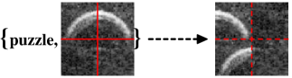
Figure 7: Jigsaw puzzle data generation. From left to right: grid generation and shuffling of patches ($2\times 2$ example).

To frame the Jigsaw algorithm as a classification problem, we associate an integer label to each permutation set. In this sense, each image is shuffled according to a given permutation order with a deterministic integer label associated to it.

4.3.2 Self-Supervised Training on Watertank Dataset

We have trained the Jigsaw model on the Watertank dataset, the original images are of size $96\times 96$. After splitting them into $3\times 3$ girds, the resulting patches are of size $32\times 32$. We used a categorical cross-entropy loss for classification, Adam optimizer, learning rate $\beta=0.001$, batches of size 128 during 20 epochs (considerably less than RotNet and DAE). We trained the same architecture for four permutation sets $\{5,10,15,20\}$ applied to the dataset separately. We summarize the pre-training results in Tab. 4. Notice that the original dimensions of the dataset increase by the permutation set size. In this case, all permutation sets yield similar test accuracies, with 5 permutations being the best performing one due to the fact that this is the minimum number of permutation sets the model has to classify.

Permutations	Test Set Size	Test Set Accuracy
5	1975	97.22%
10	3950	96.76%
15	5925	96.03%
20	7900	94.87%

Table 4: Jigsaw pre-training classification results on the test set of the Watertank dataset. Results are shown for different permutation sets.

4.3.3 Transfer Learning on Turntable Dataset

For transfer learning evaluations on the Turntable dataset, we have taken the learned weights from the feature extractor pretrained with Jigsaw. For this integration, we had to change the input size of the feature extractor to take inputs of shape $96\times 96$ corresponding to the actual image dimensions from the Turntable dataset, as the original Jigsaw model processes inputs with shapes $(9,32,32,1)$ due to the 9 patches split. Similar to RotNet and DAE, we generate embeddings for the four pretrained Jigsaw models, one for each permutation set, and subsample the training set to train an SVM classifier with parameter $C=1.0$.

In Fig. 8 we show the transfer learning for low-shot classification results on each permutation set. Similar to RotNet, we have taken three intermediate layers and evaluated their performance. Overall, the performance of the self-supervised pre-training curves is on par with the supervised pre-training curves. Similar to RotNet and DAE, lower samples per class (e.g. 10, 20, 30) yield higher variations, whereas higher samples per class have lower standard deviations and make training more stable. We have observed that the best performing Jigsaw model occurs with 10 permutations, dropout-1 layer with an accuracy of $96.83\pm 0.47\%$, this is less than 1% difference compared to the best supervised performing model with dropout-1 layer and accuracy of $97.08\pm 0.22\%$,. In Tab. 8 from Appendix G we summarize the results for all permutation sets together with the supervised learning counterpart.

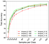
(a) 5 Permutations

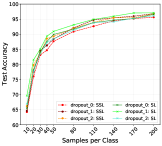
(b) 10 Permutations

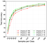
(c) 15 Permutations

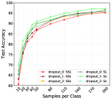
(d) 20 Permutations

Figure 8: Transfer learning evaluation on the turntable dataset with the Jigsaw model. Test accuracies are reported for varying number of permutations applied to each image in the dataset.

4.4 Self-Supervised Training on Wild Images

In addition to the pre-training studies on the Watertank dataset carried out before, we have also pretrained our models on “wild‘” uncurated sonar images. As discussed in [7], computer vision models can be more robust when pretrained on uncurated images, one of the main reasons being that there are no well-defined classes and object shapes which can lead to biased results. Furthermore, characterizing the performance of our models on wild data is crucial in order to relax the constrain of having to manually annotate sonar datasets. For this, we collected sonar images from the seabed of a lake and generated random patches out of them. Fig. 9 shows the proposed regions and the extracted patches. In total, we have generated 63,000 patches that contain different kinds of seabed shapes but no well-defined objects or shapes. We split the data into 80% training, 20% testing and trained our three proposed SSL methods with the same corresponding parameters described in the previous sections. Since this dataset has no class labels, we only trained with the synthetic labels from each self-supervised approach.

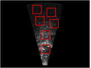
(a)

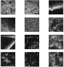
(b)

Figure 9: Random patch generation from seabed sonar images: (a) patch region proposal, (b) resulting ”wild” patches.

In Fig. 10 and Tab. 5 we summarize the best performing models for Wild and Watertank data pre-training, evaluated on the Turntable dataset (200 spc case). We observed that RotNet Wild (SSL) has an overwhelming poor performance due to the fact that the model struggles at identifying rotations from wild objects that have no well-defined form and shape. Aside from this approach, most methods with Wild pre-training have a competitive performance against Watertank pre-training (for SL and SSL). Remarkably, Jigsaw (blue bars) with Wild pre-training performed on pair with supervised pre-training, thus showing its potential for broader real-life scenarios and paving the way to tackle further tasks with sonar images and SSL approaches. In Fig. 11 from Appendix H we show further model comparisons for the case of 10, 40 and 110 spc, the behavior in these cases is similar to 200 spc.

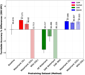
Figure 10: Comparison of baseline SVM, the best performing SSL models pretrained on the Watertank sonar dataset (with supervision and self-supervision) and the Wild sonar dataset. 200 spc case.

5 Discussion and Analysis

Across all three SSL methods, we found that, as opposed to the spc reported in [40], we have required up to 200 spc (all the dataset) in order to achieve accuracies higher than 90%. This has to do with the fact that our pre-training is done on the watertank data and our transfer learning evaluation is done on the turntable data (the opposite direction), the reason behind this can be that the turntable dataset is statistically more diverse due to the fact that rotating objects can result in slightly different sonar images due to shadows and thus harder to classify.

We observe that improvement of self-supervised pre-training is more prominent for low-shot scenarios. For example, the Jigsaw Watertank SSL and Wild SSL has an increased accuracy from the baseline by around 7% for 10 spc. As we increase these samples, the variation decreases since the baseline learns from more examples. Compared to RotNet and Jigsaw, DAE achieved considerably lower accuracies, we hypothesize that this is mainly due to the fact that this method does not increase the dataset dimensions (e.g. RotNet increases it by 4), but rather, the dataset corrupts only original images. Overall, the best performing model is Jigsaw, requiring only 20 epochs to reach competitive accuracies (against 200 epochs for RotNet and DAE). On top of this, the feature extractor used in Jigsaw has $\sim$6,000 parameters, whereas RotNet and DAE contain $\sim$1,000,000 and $\sim$200,000 parameters, respectively.

Overall we believe our results show that SSL is a viable alternative to pre-train neural networks for sonar image classification, but unlike many results in color images, SSL does not seem to improve over feature learning using supervised learning. It is encouraging for the marine robotics community that SSL can be used for pre-training, and we expect that our models and methods will be used in practice. We will release code and all self-supervised pre-trained models publicly once the paper is accepted.

Model	Accuracy	Difference to Baseline
Baseline SVM	$95.67\%$	–
Rotnet - Watertank SL	$97.27\%$	$+1.60\%$
Rotnet - Watertank SSL	$96.62\%$	$+0.95\%$
Rotnet - Wild SSL	$12.71\%$	$-82.96\%$
AE - Watertank SL	$92.22\%$	$-3.45\%$
DAE - Watertank SSL	$94.50\%$	$-1.17\%$
DAE - Wild SSL	$85.23\%$	$-10.44\%$
Jigsaw - Watertank SL	$97.09\%$	$+1.42\%$
Jigsaw - Watertank SSL	$96.84\%$	$+1.17\%$
Jigsaw - Wild SSL	$97.02\%$	$+1.35\%$

Table 5: Comparison of the baseline SVM, the pre-trained models on the Watertank sonar dataset and the Wild sonar dataset.

6 Conclusions and Future Work

In this work we evaluate three self-supervised learning algorithms for learning features from sonar images, using two datasets (marine debris turntable and on the wild sonar image patches), and evaluated them in classifying the marine debris watertank datset. These results prove that SSL methods that are commonly used for RBG images also work for sonar images and perform similarly.

Our results show that the performance of the evaluated self-supervised algorithms is on par with supervised algorithms for sonar image classification. We have verified experimentally that our algorithms can generate high-quality image embeddings for classification after a pre-training and transfer learning procedure. Across all three algorithms, the differences between SSL and SL in the obtained accuracies are small (only 1-2%), this positions self-supervised learning as a strong candidate in the absence of labeled data. We notice that Jigsaw is the best performing SSL algorithm with a best accuracy of 97.02% (surpassing RotNet with 96.46% and DAE with 94.49%), we argue that this is because this method benefits from image augmentation (synthetic labels) by design, remarkably, this result was achieved by pre-training on the wild uncurated sonar dataset, proving the potential of SSL to avoid labeling large sonar datasets (saving time and costs) and learning image representations from a diverse set of object shapes and forms.

We expect that our results increase the use of self-supervised learning for feature learning in sonar images, improving the overall autonomy and perception capabilities of underwater vehicles.

For future work, we plan to further investigate Transformer-based architectures for pre-training. We also plan to deploy some of our best performing pretrained models in real-life underwater environments for object classification. Lastly, we want to investigate further SSL techniques for the problem of image translation using multiple learning modalities (sonar and camera data).

Appendix A Data and Models Release

All training data used in this paper is available at https://github.com/mvaldenegro/marine-debris-fls-datasets/ and models and source code is available at https://github.com/agrija9/ssl-sonar-images.

Appendix B RotNet Model Selection

In this section we describe the neural network architectures that we used for evaluating RotNet.

Similar to the work in [40], we have implemented the several CNN architectures to evaluate the performance of RotNet in sonar images. All the described network architectures are lightweight versions that try to address memory and performance challenges in underwater robotics:

ResNet [10]: Uses residual connections to improve gradient propagation through the network, this feature allows to design much deeper networks. For our experiments we used a compact variant (ResNet20) which has 20 residual layers.

MobileNet [13]: It is designed to be lightweight in order to do fast inference in mobile devices. It features depthwise separable convolutions to reduce computations (this induces a trade-off between accuracy performance and computation performance).

DenseNet [14]: It reuses features heavily. It is composed by a set of dense convolutional blocks, where each of them is a series of convolutional layers, and each layer takes as inputs the feature maps from the previous convolutional layers in the same block. For our experiments, we used DenseNet121, which is the shallowest variation as described in [14].

SqueezeNet [15]: It reduces the number of parameters while maintaining competitive performance, this is achieved by designing so called Fire modules which contain two sub-modules, one squeezes information through a bottleneck and another one expands the amount of information. According to [15], SqueezeNet has similar performance to AlexNet on ImageNet but with overall 50x less parameters.

MiniXception: This network is a modification to the Xception network [4] since it reduces the amount of computation needed (e.g. for facial emotion recognition [1]). Xception is a model that combines ideas from MobileNets by using depthwise separbale convolutions.

Appendix C Detailed RotNet Transfer Learning Results

In this section we show additional detailed transfer learning results with RotNet, presented in Table 6.

Test Set Accuracy
RotNet Baseline	Layer	10 Samples	40 Samples	110 Samples	200 Samples
ResNet20 Self-Supervised ResNet20 Supervised	flatten activation 18 activation 17 flatten activation 18 activation 17	68.22 $\pm$ 1.83% 66.64 $\pm$ 2.95% 66.19 $\pm$ 2.14% 76.51 $\pm$ 3.30% 70.14 $\pm$ 4.40% 71.61 $\pm$ 3.10%	84.40 $\pm$ 1.74% 85.70 $\pm$ 0.84% 85.28 $\pm$ 1.31% 90.20 $\pm$ 1.23% 88.06 $\pm$ 1.40% 88.43 $\pm$ 1.44%	90.06 $\pm$ 1.08% 93.48 $\pm$ 0.67% 93.62 $\pm$ 0.83% 94.62 $\pm$ 0.75% 95.27 $\pm$ 0.74% 95.25 $\pm$ 0.87%	92.07 $\pm$ 0.58% 96.46 $\pm$ 0.54% 96.62 $\pm$ 0.56% 96.17 $\pm$ 0.46% 97.27 $\pm$ 0.60% 97.14 $\pm$ 0.79%
MobileNet Self-Supervised MobileNet Supervised	conv_pw_11_relu flatten conv_pw_12_relu conv_pw_11_relu flatten conv_pw_12_relu	58.21 $\pm$ 1.65% 51.08 $\pm$ 2.07% 54.97 $\pm$ 2.03% 63.90 $\pm$ 1.64% 60.04 $\pm$ 3.15% 59.98 $\pm$ 1.89%	74.66 $\pm$ 1.13% 68.32 $\pm$ 1.28% 70.63 $\pm$ 1.23% 76.38 $\pm$ 1.72% 72.10 $\pm$ 1.10% 74.35 $\pm$ 1.35%	83.86 $\pm$ 1.03% 76.68 $\pm$ 0.99% 79.30 $\pm$ 1.24% 84.09 $\pm$ 1.27% 78.80 $\pm$ 0.86% 80.40 $\pm$ 1.27%	88.14 $\pm$ 0.76% 82.35 $\pm$ 0.99% 83.31 $\pm$ 0.77% 87.34 $\pm$ 0.84% 81.64 $\pm$ 1.16% 83.69 $\pm$ 0.48%
DenseNet121 Self-Supervised DenseNet121Supervised	conv5_block15_0_relu conv5_block16_0_relu avg pool conv5_block15_0_relu conv5_block16_0_relu avg pool	67.95 $\pm$ 2.17% 68.85 $\pm$ 2.88% 64.51 $\pm$ 3.17% 69.95 $\pm$ 3.29% 68.97 $\pm$ 3.34% 63.65 $\pm$ 2.70%	85.59 $\pm$ 1.20% 86.89 $\pm$ 1.13% 80.96 $\pm$ 1.11% 86.69 $\pm$ 0.94% 86.26 $\pm$ 1.38% 81.82 $\pm$ 1.39%	92.10 $\pm$ 0.90% 92.58 $\pm$ 0.73% 88.26 $\pm$ 1.05% 93.75 $\pm$ 0.64% 93.56 $\pm$ 0.79% 88.60 $\pm$ 0.85%	95.02 $\pm$ 0.43% 94.66 $\pm$ 0.56% 90.17 $\pm$ 0.69% 95.70 $\pm$ 0.41% 95.61 $\pm$ 0.55% 91.96 $\pm$ 0.37%
SqueezeNet Self-Supervised SqueezeNet Supervised	batch_norm_8 batch_norm_9 global_average_pooling2d batch_norm_8 batch_norm_9 global_average_pooling2d	62.54 $\pm$ 2.40% 39.70 $\pm$ 2.99% 23.92 $\pm$ 2.63% 71.76 $\pm$ 2.61% 56.07 $\pm$ 2.52% 38.77 $\pm$ 2.61%	82.10 $\pm$ 0.88% 55.14 $\pm$ 1.62% 25.13 $\pm$ 0.98% 87.44 $\pm$ 1.40% 73.59 $\pm$ 0.96% 45.34 $\pm$ 1.59%	89.56 $\pm$ 0.85% 61.64 $\pm$ 1.53% 26.27 $\pm$ 0.80% 93.67 $\pm$ 0.92% 80.34 $\pm$ 1.53% 47.22 $\pm$ 1.23%	92.37 $\pm$ 0.58% 64.65 $\pm$ 1.33% 25.95 $\pm$ 0.98% 96.31 $\pm$ 0.40% 83.07 $\pm$ 0.84% 48.20 $\pm$ 1.15%
Minixception Self-Supervised Minixception Supervised	add_3 add_2 conv2d_6 add_3 add_2 conv2d_6	68.63 $\pm$ 2.13% 66.71 $\pm$ 2.28% 52.74 $\pm$ 2.43% 71.33 $\pm$ 3.39% 70.34 $\pm$ 2.23% 64.24 $\pm$ 3.36%	82.94 $\pm$ 1.41% 85.78 $\pm$ 1.21% 65.75 $\pm$ 1.48% 88.38 $\pm$ 0.97% 87.98 $\pm$ 0.96% 79.87 $\pm$ 1.20%	90.12 $\pm$ 0.73% 92.80 $\pm$ 1.01% 70.91 $\pm$ 1.01% 94.34 $\pm$ 0.83% 94.63 $\pm$ 0.77% 86.68 $\pm$ 1.17%	92.29 $\pm$ 0.70% 95.30 $\pm$ 0.51% 73.73 $\pm$ 0.95% 96.86 $\pm$ 0.46% 96.91 $\pm$ 0.68% 89.39 $\pm$ 0.56%
Linear SVM	NA	63.55 $\pm$ 3.66%	85.39 $\pm$ 1.07%	92.51 $\pm$ 0.79%	95.67 $\pm$ 0.90%

Table 6: RotNet transfer learning classification accuracies on the Turntable dataset.

Appendix D Denoising Autoencoder Model Selection

In this section we describe the neural network architecture that we used as a Denoising Autoencoder.

We selected the following encoder-decoder CNN architecture for the DAE, which based on the one reported in [40]: The encoder architecture consists of Conv2D(32, $3\times 3$) - MaxPool($2\times 2$) - Conv2D(16, $3\times 3$) - MaxPool($2\times 2$) - Conv2D(8, $3\times 3$) - MaxPool($2\times 2$) - Flatten() - Fully Connected(c). The decoder architecture is composed by Fully Connected($c\times n_{w}\times n_{h}$) - Reshape() - Conv2D(32, $3\times 3$) - UpSample($2\times 2$) - Conv2D(16, $3\times 3$) - UpSample($2\times 2$) - Conv2D(8, $3\times 3$) - UpSample($2\times 2$) - Conv2D(1, $3\times 3$).

Appendix E Denoising Autencoder Transfer Learning Results

In this section we show additional detailed transfer learning results with a Denoising Autoencoder, presented in Table 7.

Test Set Accuracy
Model	Code Size	Gaussian Noise ($\sigma$)	10 Samples	40 Samples	110 Samples	200 Samples
Denoising AE	32	0.100 0.125 0.150 0.175 0.200	64.40 $\pm$ 2.98% 62.29 $\pm$ 1.55% 60.89 $\pm$ 2.62% 63.03 $\pm$ 3.32% 61.59 $\pm$ 2.35%	80.01 $\pm$ 1.72% 75.42 $\pm$ 1.02% 68.91 $\pm$ 1.82% 77.28 $\pm$ 1.11% 74.21 $\pm$ 2.13%	82.68 $\pm$ 1.20% 78.37 $\pm$ 0.84% 71.73 $\pm$ 0.75% 81.20 $\pm$ 1.21% 79.16 $\pm$ 1.17%	84.49 $\pm$ 0.64% 79.48 $\pm$ 1.00% 72.55 $\pm$ 1.18% 82.62 $\pm$ 0.85% 80.40 $\pm$ 1.15%
	64	0.100 0.125 0.150 0.175 0.200	64.97 $\pm$ 1.80% 61.81 $\pm$ 2.59% 67.90 $\pm$ 2.80% 63.93 $\pm$ 3.15% 62.18 $\pm$ 1.92%	83.34 $\pm$ 1.47% 78.06 $\pm$ 1.24% 81.44 $\pm$ 1.72% 79.70 $\pm$ 1.95% 79.84 + - 1.69%	88.06 $\pm$ 0.81% 82.71 $\pm$ 1.29% 86.79 $\pm$ 0.91% 85.84 $\pm$ 0.80% 85.05 $\pm$ 1.23%	89.65 $\pm$ 0.71% 85.11 $\pm$ 1.0% 88.40 $\pm$ 0.66% 87.45 $\pm$ 0.77% 86.69 $\pm$ 0.63%
	128	0.100 0.125 0.150 0.175 0.200	68.31 $\pm$ 1.60% 65.05 $\pm$ 2.98% 69.39 $\pm$ 2.24% 69.81 $\pm$ 2.31% 66.88 $\pm$ 2.98%	85.28 $\pm$ 1.32% 83.42 $\pm$ 1.61% 85.38 $\pm$ 1.60% 86.82 $\pm$ 0.97% 84.51 $\pm$ 1.52%	91.14 $\pm$ 1.09% 88.94 $\pm$ 1.22% 92.40 $\pm$ 0.87% 92.37 $\pm$ 0.78% 91.48 $\pm$ 0.60%	94.31 $\pm$ 0.63% 90.07 $\pm$ 0.90% 94.49 $\pm$ 0.62% 93.96 $\pm$ 0.73% 93.73 $\pm$ 0.94%
AE	32	-	67.53 $\pm$ 2.03%	81.56 $\pm$ 1.55%	86.54 $\pm$ 1.13%	88.31 $\pm$ 0.83%
	64	-	67.10 $\pm$ 3.01%	83.84 $\pm$ 1.54%	89.16 $\pm$ 0.92%	91.39 $\pm$ 0.53%
	128	-	67.86 $\pm$ 1.53%	83.25 $\pm$ 1.59%	90.54 $\pm$ 1.30%	92.21 $\pm$ 0.59%

Table 7: Denoising Autoencoder transfer learning classification accuracies on the Turntable dataset.

Appendix F Jigsaw Model Selection

In this section we describe the neural network architecture that we used for Jigsaw self-supervised learning.

Extensive experiments were carried out to optimize the CNN feature extractor design that works as a baseline for Jigsaw. The main parameters that we varied were the number of layers, number of filters and downsampling in the feature extractor. The original Jigsaw architecture [30] uses a set of $\{64,128,256,386\}$ 2DConvs. In our case, we have reduced considerably the number these filters (and hence number of parameters) to a set of $\{32,16,8\}$ 2DConvs, this is because our Jigsaw model is trained on the smaller Watertank dataset and such large models might lead easily to overfitting.

We used a Time Distributed Layer (TDL) from Keras in order to feed image patches simultaneously through the sequential CNN feature extractor and a final decision network (classification layer). The feature extractor is composed of the following layers: Conv2D(32, $3\times 3$) - BatchNorm() - MaxPool($2\times 2$) - Dropout() - Conv2D(16, $3\times 3$) - BatchNorm() - MaxPool($2\times 2$) - Dropout() - Conv2D(8, $3\times 3$) -BatchNorm() - MaxPool($2\times 2$)- Dropout() - Flatten(). The TDL takes this sequential model and flattens the output predictions from every image tile to then process them through the decision network. The decision network is composed by: TimeDistributedLayer(9, None) - Flatten() - FullyConnected() - BatchNorm() - FullyConnected() - BatchNorm() - Dropout() - FullyConnected().

Appendix G Jigsaw Transfer Learning Results

In this section we show additional detailed transfer learning results with Jigsaw, presented in Table 8.

Test Set Accuracy
Permutations	Layer	10 Samples	40 Samples	110 Samples	200 Samples
5	dropout_0	60.61 $\pm$ 1.68%	83.93 $\pm$ 1.25%	91.59 $\pm$ 0.63%	95.19 $\pm$ 1.09%
	dropout_1	66.41 $\pm$ 2.67%	86.17 $\pm$ 1.06%	94.51 $\pm$ 0.95%	96.74 $\pm$ 0.66%
	dropout_2	70.14 $\pm$ 2.36%	86.76 $\pm$ 2.10%	94.35 $\pm$ 1.16%	96.24 $\pm$ 0.47%
10	dropout_0	64.248 $\pm$ 2.22%	84.71 $\pm$ 1.79%	92.65 $\pm$ 1.44%	95.62 $\pm$ 0.74%
	dropout_1	64.62 $\pm$ 1.75%	86.29 $\pm$ 1.85%	94.76 $\pm$ 0.74%	96.83 $\pm$ 0.47 %
	dropout_2	66.20 $\pm$ 1.51%	88.55 $\pm$ 0.78%	93.95 $\pm$ 1.41%	96.77 $\pm$ 0.41%
15	dropout_0	64.0 $\pm$ 3.88%	84.40 $\pm$ 0.98%	91.84 $\pm$ 1.13%	95.16 $\pm$ 0.50%
	dropout_1	67.10 $\pm$ 1.68%	86.73 $\pm$ 1.66%	94.51 $\pm$ 1.07%	96.65 $\pm$ 0.46%
	dropout_2	68.18 $\pm$ 4.74%	85.73 $\pm$ 2.09%	93.79 $\pm$ 0.68%	95.93 $\pm$ 0.58%
20	dropout_0	60.71 $\pm$ 2.55%	83.59 $\pm$ 0.73%	91.84 $\pm$ 0.77%	95.19 $\pm$ 0.39%
	dropout_1	63.16 $\pm$ 1.89%	85.36 $\pm$ 1.51%	93.55 $\pm$ 0.63%	95.62 $\pm$ 0.87%
	dropout_2	67.25 $\pm$ 2.57%	87.16 $\pm$ 1.34%	93.36 $\pm$ 0.72%	95.59 $\pm$ 0.52%
Supervised	dropout_0	65.45 $\pm$ 2.96%	87.59 $\pm$ 1.51%	93.82 $\pm$ 1.05%	96.58 $\pm$ 0.59%
	dropout_1	69.64 $\pm$ 3.99%	89.33 $\pm$ 1.09%	94.91 $\pm$ 0.85%	97.08 $\pm$ 0.22%
	dropout_2	66.94 $\pm$ 1.26%	87.25 $\pm$ 1.46%	93.89 $\pm$ 1.51%	96.09 $\pm$ 0.51%

Table 8: Jigsaw transfer learning classification accuracies on the Turntable dataset.

Appendix H Comparison of Best Performing Transfer Learning Models

In this section we show additional comparisons of the best transfer learning results, presented in Figure 11 for selected values of samples per class (SPC).

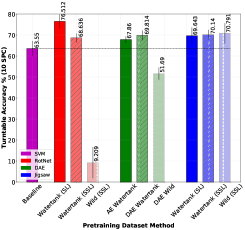
(a) 10 spc.

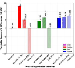
(b) 10 spc with baseline substracted.

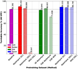
(c) 40 spc

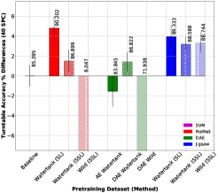
(d) 40 spc with baseline substracted.

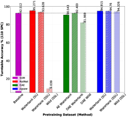
(e) 110 spc

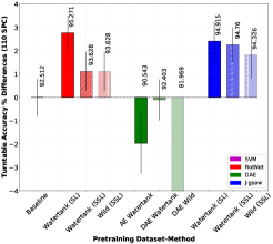
(f) 110 spc with baseline substracted.

Figure 11: Comparison of the best performing SSL models pretrained on the Watertank sonar dataset (with supervision and self-supervision) and the Wild sonar dataset. 10, 40 and 110 spc cases.

References

- [1] Octavio Arriaga, Matias Valdenegro-Toro, and Paul Plöger. Real-time convolutional neural networks for emotion and gender classification. arXiv preprint arXiv:1710.07557, 2017.
- [2] Mathilde Caron, Ishan Misra, Julien Mairal, Priya Goyal, Piotr Bojanowski, and Armand Joulin. Unsupervised learning of visual features by contrasting cluster assignments. In H. Larochelle, M. Ranzato, R. Hadsell, M. F. Balcan, and H. Lin, editors, Advances in Neural Information Processing Systems, volume 33, pages 9912–9924. Curran Associates, Inc., 2020.
- [3] Ting Chen, Simon Kornblith, Mohammad Norouzi, and Geoffrey Hinton. A simple framework for contrastive learning of visual representations. In Hal Daumé III and Aarti Singh, editors, Proceedings of the 37th International Conference on Machine Learning, volume 119 of Proceedings of Machine Learning Research, pages 1597–1607. PMLR, 13–18 Jul 2020.
- [4] Francois Chollet. Xception: Deep learning with depthwise separable convolutions. 2017 IEEE Conference on Computer Vision and Pattern Recognition (CVPR), pages 1800–1807, 2017.
- [5] Zeyu Feng, Chang Xu, and Dacheng Tao. Self-supervised representation learning by rotation feature decoupling. In Proceedings of the IEEE/CVF Conference on Computer Vision and Pattern Recognition (CVPR), June 2019.
- [6] Spyros Gidaris, Praveer Singh, and Nikos Komodakis. Unsupervised representation learning by predicting image rotations, 2018.
- [7] Priya Goyal, Quentin Duval, Isaac Seessel, Mathilde Caron, Mannat Singh, Ishan Misra, Levent Sagun, Armand Joulin, and Piotr Bojanowski. Vision models are more robust and fair when pretrained on uncurated images without supervision. arXiv preprint arXiv:2202.08360, 2022.
- [8] Priya Goyal, Dhruv Mahajan, Abhinav Gupta, and Ishan Misra. Scaling and benchmarking self-supervised visual representation learning. In Proceedings of the IEEE/CVF International Conference on Computer Vision (ICCV), October 2019.
- [9] Jean-Bastien Grill, Florian Strub, Florent Altché, Corentin Tallec, Pierre Richemond, Elena Buchatskaya, Carl Doersch, Bernardo Avila Pires, Zhaohan Guo, Mohammad Gheshlaghi Azar, Bilal Piot, koray kavukcuoglu, Remi Munos, and Michal Valko. Bootstrap your own latent - a new approach to self-supervised learning. In H. Larochelle, M. Ranzato, R. Hadsell, M. F. Balcan, and H. Lin, editors, Advances in Neural Information Processing Systems, volume 33, pages 21271–21284. Curran Associates, Inc., 2020.
- [10] Kaiming He, Xiangyu Zhang, Shaoqing Ren, and Jian Sun. Deep residual learning for image recognition. In Proceedings of the IEEE conference on computer vision and pattern recognition, pages 770–778, 2016.
- [11] Olivier Henaff. Data-efficient image recognition with contrastive predictive coding. In Hal Daumé III and Aarti Singh, editors, Proceedings of the 37th International Conference on Machine Learning, volume 119 of Proceedings of Machine Learning Research, pages 4182–4192. PMLR, 13–18 Jul 2020.
- [12] Dan Hendrycks, Mantas Mazeika, Saurav Kadavath, and Dawn Song. Using self-supervised learning can improve model robustness and uncertainty. In Advances in Neural Information Processing Systems, volume 32. Curran Associates, Inc., 2019.
- [13] Andrew G Howard, Menglong Zhu, Bo Chen, Dmitry Kalenichenko, Weijun Wang, Tobias Weyand, Marco Andreetto, and Hartwig Adam. Mobilenets: Efficient convolutional neural networks for mobile vision applications. arXiv preprint arXiv:1704.04861, 2017.
- [14] Gao Huang, Zhuang Liu, Laurens van der Maaten, and Kilian Q Weinberger. Densely connected convolutional networks. In Proceedings of the IEEE Conference on Computer Vision and Pattern Recognition, 2017.
- [15] Forrest N Iandola, Song Han, Matthew W Moskewicz, Khalid Ashraf, William J Dally, and Kurt Keutzer. Squeezenet: Alexnet-level accuracy with 50x fewer parameters and¡ 0.5 mb model size. arXiv preprint arXiv:1602.07360, 2016.
- [16] Satoshi Iizuka, Edgar Simo-Serra, and Hiroshi Ishikawa. Globally and locally consistent image completion. ACM Trans. Graph., 36(4), July 2017.
- [17] Ashish Jaiswal, Ashwin Ramesh Babu, Mohammad Zaki Zadeh, Debapriya Banerjee, and Fillia Makedon. A survey on contrastive self-supervised learning. Technologies, 9(1):2, 2021.
- [18] Hyesu Jang, Giseop Kim, Yeongjun Lee, and Ayoung Kim. Cnn-based approach for opti-acoustic reciprocal feature matching. In ICRA Workshop on Underwater Robotics Perception, 2019.
- [19] Longlong Jing and Yingli Tian. Self-supervised visual feature learning with deep neural networks: A survey. IEEE transactions on pattern analysis and machine intelligence, 43(11):4037–4058, 2020.
- [20] Juhwan Kim, Seokyong Song, and Son-Cheol Yu. Denoising auto-encoder based image enhancement for high resolution sonar image. In 2017 IEEE underwater technology (UT), pages 1–5. IEEE, 2017.
- [21] Diederik Kingma and Jimmy Ba. Adam: A method for stochastic optimization. International Conference on Learning Representations, 12 2014.
- [22] Gustav Larsson, Michael Maire, and Gregory Shakhnarovich. Colorization as a proxy task for visual understanding. In Proceedings of the IEEE conference on computer vision and pattern recognition, pages 6874–6883, 2017.
- [23] Christian Ledig, Lucas Theis, Ferenc Huszár, Jose Caballero, Andrew Cunningham, Alejandro Acosta, Andrew Aitken, Alykhan Tejani, Johannes Totz, Zehan Wang, et al. Photo-realistic single image super-resolution using a generative adversarial network. In Proceedings of the IEEE conference on computer vision and pattern recognition, pages 4681–4690, 2017.
- [24] Hsin-Ying Lee, Jia-Bin Huang, Maneesh Singh, and Ming-Hsuan Yang. Unsupervised representation learning by sorting sequences. In Proceedings of the IEEE international conference on computer vision, pages 667–676, 2017.
- [25] Meng Li, William Hsu, Xiaodong Xie, Jason Cong, and Wen Gao. Sacnn: Self-attention convolutional neural network for low-dose ct denoising with self-supervised perceptual loss network. IEEE Transactions on Medical Imaging, 39(7):2289–2301, 2020.
- [26] Ru Li, Shuaicheng Liu, Guangfu Wang, Guanghui Liu, and Bing Zeng. Jigsawgan: Auxiliary learning for solving jigsaw puzzles with generative adversarial networks. IEEE Transactions on Image Processing, 31:513–524, 2021.
- [27] Xiao Liu, Fanjin Zhang, Zhenyu Hou, Li Mian, Zhaoyu Wang, Jing Zhang, and Jie Tang. Self-supervised learning: Generative or contrastive. IEEE Transactions on Knowledge and Data Engineering, 2021.
- [28] Ishan Misra and Laurens van der Maaten. Self-supervised learning of pretext-invariant representations. In Proceedings of the IEEE/CVF Conference on Computer Vision and Pattern Recognition (CVPR), June 2020.
- [29] Ishan Misra, C Lawrence Zitnick, and Martial Hebert. Shuffle and learn: unsupervised learning using temporal order verification. In European Conference on Computer Vision, pages 527–544. Springer, 2016.
- [30] Mehdi Noroozi and Paolo Favaro. Unsupervised learning of visual representations by solving jigsaw puzzles. In European conference on computer vision, pages 69–84. Springer, 2016.
- [31] Deepak Pathak, Philipp Krahenbuhl, Jeff Donahue, Trevor Darrell, and Alexei A Efros. Context encoders: Feature learning by inpainting. In Proceedings of the IEEE conference on computer vision and pattern recognition, pages 2536–2544, 2016.
- [32] Augustin-Alexandru Saucan, Christophe Sintes, Thierry Chonavel, and Jean-Marc Le Caillec. Model-based adaptive 3d sonar reconstruction in reverberating environments. IEEE transactions on image processing, 24(10):2928–2940, 2015.
- [33] Nitish Srivastava, Elman Mansimov, and Ruslan Salakhudinov. Unsupervised learning of video representations using lstms. In International conference on machine learning, pages 843–852. PMLR, 2015.
- [34] Vladimiros Sterzentsenko, Leonidas Saroglou, Anargyros Chatzitofis, Spyridon Thermos, Nikolaos Zioulis, Alexandros Doumanoglou, Dimitrios Zarpalas, and Petros Daras. Self-supervised deep depth denoising. In Proceedings of the IEEE/CVF International Conference on Computer Vision (ICCV), October 2019.
- [35] Minsung Sung, Hyeonwoo Cho, Hangil Joe, Byeongjin Kim, and Son-Choel Yu. Crosstalk noise detection and removal in multi-beam sonar images using convolutional neural network. In OCEANS 2018 MTS/IEEE Charleston, pages 1–6, 2018.
- [36] Aiham Taleb, Christoph Lippert, Tassilo Klein, and Moin Nabi. Multimodal self-supervised learning for medical image analysis. In International Conference on Information Processing in Medical Imaging, pages 661–673. Springer, 2021.
- [37] Kei Terayama, Kento Shin, Katsunori Mizuno, and Koji Tsuda. Integration of sonar and optical camera images using deep neural network for fish monitoring. Aquacultural Engineering, 86:102000, 2019.
- [38] Matias Valdenegro-Toro. Object recognition in forward-looking sonar images with convolutional neural networks. In OCEANS 2016 MTS/IEEE Monterey, pages 1–6, 2016.
- [39] Matias Valdenegro-Toro. Best practices in convolutional networks for forward-looking sonar image recognition. In OCEANS 2017-Aberdeen, pages 1–9. IEEE, 2017.
- [40] Matias Valdenegro-Toro, Alan Preciado-Grijalva, and Bilal Wehbe. Pre-trained models for sonar images. In OCEANS 2021: San Diego – Porto, pages 1–8, 2021.
- [41] Pascal Vincent, Hugo Larochelle, Yoshua Bengio, and Pierre-Antoine Manzagol. Extracting and composing robust features with denoising autoencoders. In Proceedings of the 25th International Conference on Machine Learning, ICML ’08, page 1096–1103, New York, NY, USA, 2008. Association for Computing Machinery.
- [42] Xingmei Wang, Jia Jiao, Jingwei Yin, Wensheng Zhao, Xiao Han, and Boxuan Sun. Underwater sonar image classification using adaptive weights convolutional neural network. Applied Acoustics, 146:145–154, 2019.
- [43] Yaochen Xie, Zhengyang Wang, and Shuiwang Ji. Noise2same: Optimizing a self-supervised bound for image denoising. In H. Larochelle, M. Ranzato, R. Hadsell, M. F. Balcan, and H. Lin, editors, Advances in Neural Information Processing Systems, volume 33, pages 20320–20330. Curran Associates, Inc., 2020.
- [44] Richard Zhang, Phillip Isola, and Alexei A Efros. Colorful image colorization. In European conference on computer vision, pages 649–666. Springer, 2016.
- [45] Richard Zhang, Jun-Yan Zhu, Phillip Isola, Xinyang Geng, Angela S. Lin, Tianhe Yu, and Alexei A. Efros. Real-time user-guided image colorization with learned deep priors. ACM Trans. Graph., 36(4), jul 2017.