Learning to Constrain Policy Optimization with Virtual Trust Region

Abstract

We introduce a constrained optimization method for policy gradient reinforcement learning, which uses a virtual trust region to regulate each policy update. In addition to using the proximity of one single old policy as the normal trust region, we propose forming a second trust region through another virtual policy representing a wide range of past policies. We then enforce the new policy to stay closer to the virtual policy, which is beneficial if the old policy performs poorly. More importantly, we propose a mechanism to automatically build the virtual policy from a memory of past policies, providing a new capability for dynamically learning appropriate virtual trust regions during the optimization process. Our proposed method, dubbed Memory-Constrained Policy Optimization (MCPO), is examined in diverse environments, including robotic locomotion control, navigation with sparse rewards and Atari games, consistently demonstrating competitive performance against recent on-policy constrained policy gradient methods.

1 Introduction

Deep reinforcement learning (RL) is the current workhorse in machine learning. Using neural networks to approximate value and policy functions enables classical approaches such as Q-learning Watkins and Dayan (1992) and policy gradient Sutton et al. (2000) to achieve promising results on many challenging problems such as Go, Atari games and robotics Silver et al. (2017); Mnih et al. (2015); Lillicrap et al. (2016); Mnih et al. (2016). Compared to Deep Q-learning, deep policy gradient (PG) methods are often more flexible and applicable to discrete and continuous action problems. However, these methods tend to suffer from high sample complexity and training instability since the gradient may not accurately reflect the policy gain when the policy changes substantially Kakade and Langford (2002). This is exacerbated for deep policy networks where numerous parameters need to be optimized, and minor updates in parameter space can lead to considerable changes in policy space.

To address this issue, one solution is to regularize each policy update by restricting the Kullback–Leibler (KL) divergence between the new policy and the previous one, which can guarantee monotonic policy improvement Schulman et al. (2015a). However, jointly optimizing the approximate advantage function and the KL term does not work in practice Schulman et al. (2015a). Therefore, Schulman et al. (2015) proposed Trust Region Policy Optimization (TRPO) to constrain the new policy within a KL divergence radius, which requires second-order gradients. Alternatives such as Proximal Policy Optimization (PPO) Schulman et al. (2017) use a simpler first-order optimization with adaptive KL or clipped surrogate objective while still maintaining the reliable performance of TRPO. Recent methods recast the problem through a new lens using Expectation-Maximization or Mirror Descent Optimization, and this also results in first-order optimization with KL divergence term in the loss function Abdolmaleki et al. (2018); Song et al. (2019); Yang et al. (2019); Tomar et al. (2020).

An issue with the above methods is that the previous policy used to restrict the new policy may be suboptimal and thus unreliable in practice. For example, due to stochasticity and approximations, the new policy may fall into a local optimum even under trust-region optimizations. Then in the next update, this policy will become the “previous” policy, and will continue pulling the next policy to stay in the local optimum, thus slowing down the training progress. For on-policy methods using mini-batch updates like PPO, the situation is more problematic as the “previous” policy is defined as the old policy to collect data, which can be either very far or close to the current policy. There is no guarantee that the old policy defines a reasonable trust region for regulating the new policy.

In this paper, we propose a novel constrained policy iteration procedure, dubbed Memory-Constrained Policy Optimization (MCPO), wherein a virtual policy representing memory of past policies regularizes each policy update. The virtual policy forms a virtual trust region, attracting the new policy more when the old policy performs badly, which prevents the optimization from falling into local optimum caused by the old policy of poor quality. As such, we measure 2 KL divergences corresponding to the virtual and old policy, and assign different weights to the two KL terms in building the objective function. The weights are computed dynamically based on the performance of the two policies (the higher performer yields higher weights).

In contrast to prior works using heuristics (e.g. running average or mean of past policies) to form additional trust regions Wang et al. (2016), we argue that the virtual policy should be determined dynamically to maximize the performance on current training data. Thus we store policies in a policy memory, and learn to extract the most relevant ones to the current context. We sum the past policies in a weighted manner wherein the weights are generated by a neural network–named the attention network, which takes the information of the current, the old and the last virtual policy as the input. The attention network is optimized to maximize the approximate expected advantages of the virtual policy. We jointly optimize the policy and attention networks to train our system, alternating between sampling data from the policy and updating the networks in a mini-batch manner.

We verify our proposed MCPO through a diverse set of experiments and compare our performance with that of recent constrained policy optimization baselines. In our experiment on classical control tasks, amongst tested models, MCPO consistently achieves better performance across tasks and hyperparameters. Our testbed on 6 Mujoco tasks shows that MCPO with a big policy memory is performant where the attention network plays an important role. We also demonstrate MCPO’s capability of learning efficiently on sparse reward and high-dimensional problems such as navigation and Atari games. Finally, our ablation study highlights the necessity of MCPO’s components such as the virtual policy and the attention network.

2 Background: Policy Optimization with Trust Region

In this section, we briefly review some fundamental constrained policy optimization approaches. A general idea is to force the new policy $\pi_{\theta}$ to be close to a recent policy $\pi_{\theta_{old}}$. In this paper, we usually refer to a policy via its parameters (i.e. policy $\theta$ means policy $\pi_{\theta}$). We also use finite-horizon estimators for the advantage with discount factor $\gamma\in\left(0,1\right)$ and horizon $T$.

Conservative Policy Iteration (CPI) This method starts with a basic objective of policy gradient algorithms, which is to maximize the expected advantage $\hat{A}_{t}$.

$$L^{CPI}\left(\theta\right)=\hat{\mathbb{E}}_{t}\left[\frac{\pi_{\theta}\left(a_{t}|s_{t}\right)}{\pi_{\theta_{old}}\left(a_{t}|s_{t}\right)}\hat{A}_{t}\right]$$

where the advantage $\hat{A}_{t}$ is a function of returns collected from $\left(s_{t},a_{t}\right)$ by using $\pi_{\theta_{old}}$ (see Appendix A.2) and $\hat{\mathbb{E}}_{t}\left[\cdot\right]$ indicates the empirical average over a finite batch of data. To constrain policy updates, the new policy is a mixture of the old and the greedy policy: $\tilde{\theta}=\mathrm{argmax\;}L^{CPI}\left(\theta\right)$. That is, $\theta=\alpha\theta_{old}+(1-\alpha)\text{$\tilde{\theta}$}$ where $\alpha$ is the mixture hyperparameter Kakade and Langford (2002). As the data is sampled from the previous iteration’s policy $\theta_{old}$, the objective needs importance sampling estimation. Hereafter, we denote $\frac{\pi_{\theta}\left(a_{t}|s_{t}\right)}{\pi_{\theta_{old}}\left(a_{t}|s_{t}\right)}$ as $\tau_{t}\left(\theta\right)$ for short.

KL-Regularized Policy Optimization To enforce the constraint, one can jointly maximize the advantage and minimize KL divergence between the new and old policy, which ensures monotonic improvement Schulman et al. (2015a).

$$L^{KL}\left(\theta\right)=\hat{\mathbb{E}}_{t}\left[\tau_{t}\left(\theta\right)\hat{A}_{t}-\beta KL\left[\pi_{\theta_{old}}\left(\cdot|s_{t}\right),\pi_{\theta}\left(\cdot|s_{t}\right)\right]\right]$$

where $\beta$ is a hyperparameter that controls the update conservativeness, which can be fixed (KL Fixed) or changed (KL Adaptive) during training Schulman et al. (2017).

Trust Region Policy Optimization (TRPO) The method optimizes the expected advantage with hard constraint Schulman et al. (2015a). This is claimed as a practical implementation, less conservative than the theoretically justified algorithm using KL regularizer mentioned above.

$$L^{TRPO}\left(\theta\right) =\hat{\mathbb{E}}_{t}\left[\tau_{t}\left(\theta\right)\hat{A}_{t}\right]$$

$$\mathrm{st\>\,}\delta \geq KL\left[\pi_{\theta_{old}}\left(\cdot|s_{t}\right),\pi_{\theta}\left(\cdot|s_{t}\right)\right]$$

where $\delta$ is the KL constraint radius.

Proximal Policy Optimization (PPO) PPO is a family of constrained policy optimization, which uses first-order optimization and mini-batch updates including KL Adaptive and clipped PPO. In this paper, we use PPO to refer to the method that limits the change in policy by clipping the loss function (clipped PPO) Schulman et al. (2017). The objective $L^{PPO}$ is defined as

$$\hat{\mathbb{E}}_{t}\left[\min\left(\tau_{t}\left(\theta\right)\hat{A}_{t},\mathrm{clip}\left(\tau_{t}\left(\theta\right),1-\epsilon,1+\epsilon\right)\hat{A}_{t}\right)\right]$$

where $\epsilon$ is the clip hyperparameter.

In all the above methods, $\theta$ is the currently optimized policy, which is also referred to as the current policy. $\theta_{old}$ represents a past policy, which can be one or many update steps before the current policy. In either case, the rule to decide $\theta_{old}$ is fixed throughout training. If $\theta_{old}$ is suboptimal, it is unavoidable that the following updates will be negatively impacted. We will address this issue in the next section.

3 Memory-Constrained Policy Optimization

In trust-region policy gradient methods with mini-batch updates such as PPO, the old policy $\theta_{old}$ is often the last “sampling” policy for collecting observations from the environment. This policy is, by design, fixed during updates of the main policy until the next interaction with the environment. This means $\theta_{old}$ may not immediately precede the current policy $\theta$ but may be from many (update) steps before. Since $\theta_{old}$ is not up-to-date and could possibly be not good, using it to constrain the current policy $\theta$ can cause the suboptimal update of $\theta$. Similarly, the immediately preceding policy could also be poor in quality and thus, using it as $\theta_{old}$ could be detrimental to the optimization.

To tackle this issue, we propose to learn to constrain $\theta$ towards a weighted combination of multiple past policies besides $\theta_{old}$. We argue that we can optimize the attention network to ensure the combined policy is optimal. Below is formal description of our method.

0:  A policy buffer $\mathcal{M}$, an initial policy $\pi_{\theta_{old}}$. $T$, $K$, $B$ are the learning horizon, number of update epochs, and batch size, respectively.

1:  Initialize $\psi_{old}\leftarrow\theta_{old}$, $\theta\leftarrow\theta_{old}$

2:  for $iteration=1,2,...$ do

3:     Run policy $\pi_{\theta_{old}}$ in environment for $T$ timesteps. Compute advantage estimates $\hat{A}_{1}$, …, $\hat{A}_{T}$

4:     for $epoch=1,2,...K$ do

5:        for $batch=1,2,...T/B$ do

6:           Compute $\psi$ (Eq. 1) using $\psi_{old}$, $\theta$, $\theta_{old}$, optimize $\theta$ and $\varphi$ by maximizing $L^{MCPO}$ (Eq. 6)

7:           $\mathbf{if}$ $D\left(\theta,\psi\right)>D\left(\theta_{old},\psi\right)$ $\mathbf{then}$ add $\theta$ to $\mathcal{M}$

8:           $\mathbf{if}$ $|\mathcal{M}|>N$ $\mathbf{then}$ remove the oldest item in $\mathcal{M}$

9:           $\psi_{old}\leftarrow\psi$

10:        end for

11:     end for

12:     $\theta_{old}\leftarrow\theta$

13:  end for

Algorithm 1 Memory-Constrained Policy Optimization.

3.1 Virtual Policy

Computing the virtual policy via past policies

The virtual policy should be determined based on the past policies and their contexts such as quality, distance or entropy. A simple strategy such as taking average of past policies is likely suboptimal as the quality of these policies vary and some can be irrelevant to the current learning context. Let $\psi$ be the weighted combination of $M$ past policies $\left\{\theta_{i}\right\}_{i=1}^{M}$, which we refer to as a “virtual” policy for naming convenience, $\psi$ is computed as follows:

$$\psi=\sum_{i=1}^{M}f_{\varphi}(v)_{i}\theta_{i}$$ (1)

where $f_{\varphi}$ is a neural network parameterized by $\varphi$ which outputs softmax attention weights over the $M$ past policies, $v$ is a “context” vector capturing different relations among the current policy $\theta$, the last sampling policy $\theta_{old}$, and the last virtual policy $\psi_{old}$. We build the context by extracting specific features: pair-wise distances between policies, the empirical returns of these policies, policy entropy and value losses (details in Appendix Table 4). Intuitively, these features suggest which virtual policy will yield high performance (e.g., a virtual policy that is closer to the policy that obtained high return and low value loss). The details of $f_{\varphi}$ training will be given in Sec. 3.2.

Storing past policies with diversity-promoting writing

We use a memory buffer $\mathcal{M}$ to store past policies. We treat $\mathcal{M}$ as a queue with maximum capacity $N$, which means a new policy $\theta$ will be added to the end of $\mathcal{M}$ and if $\mathcal{M}$ is full, the oldest policy will be discarded. However, we do not add any new policy $\theta$ to $\mathcal{M}$ unconditionally but only when $\theta$ satisfies our “diversity-promoting” condition. Let $D\left(a,b\right)=\hat{\mathbb{E}}_{t}\left[KL\left[\pi_{a}\left(\cdot|s_{t}\right),\pi_{b}\left(\cdot|s_{t}\right)\right]\right]$ denote the “distance” between 2 policies $\pi_{a}$ and $\pi_{b}$, the diversity-promoting writing is defined as:

Adding $$\theta \mathcal{M} D(\theta,\psi)\geq D(\theta_{old},\psi)$$ to if (2)

where $D(\theta_{old},\psi)$ serves as a threshold. This condition makes sure that the policy to be added is far enough from $\psi$. It is reasonable because if $\theta$ is too similar to $\psi$ (in regard of $\theta_{old}$), the advantage of storing multiples past policies in order to find a good one will disappear. We will elaborate more on this in Sec. 4.5.

3.2 Policy Optimization with Two Trust Regions

Optimizing the policy parameters $\theta$

During policy optimization, we make use of both $\theta_{old}$ and $\psi$ to constrain $\theta$. Hence, $\theta_{old}$ and $\psi$ form 2 trust regions, and we aim to enforce the new policy to be closer to the better one. To this end, we propose to learn a new policy $\theta$ by maximizing the following objective function:

$$L_{1}(\theta)= \hat{\mathbb{E}}_{t}\left[\tau_{t}(\theta)\hat{A}_{t}\right]$$

$$-\beta\hat{\mathbb{E}}_{t}\bigg{[}\left(1-\alpha_{t}\left(\cdot|s_{t}\right)\right)KL\left[\pi_{\theta_{old}}\left(\cdot|s_{t}\right),\pi_{\theta}\left(\cdot|s_{t}\right)\right]$$

$$\ \ \ \ \ \ \ \ +\alpha_{t}\left(\cdot|s_{t}\right)KL\left[\pi_{\psi}\left(\cdot|s_{t}\right),\pi_{\theta}\left(\cdot|s_{t}\right)\right]\bigg{]}$$ (3)

where $\beta$ is the weight balancing between the main objective and the policy constraints, $\alpha_{t}$ is the weight balancing between constraining $\theta$ towards $\psi$ and $\theta$ towards $\theta_{old}$. The expectation is estimated by taking average over $t$ in a mini-batch of sampled data. We note that in the early stage of learning, the attention network is not trained well, and thus the quality of the virtual policy $\psi$ may be worse than $\theta_{old}$. In the long-term, $\psi$ will get better and tend to provide a better trust-region. Hence, we need to use both trust regions to ensure maximal performance at any learning stage. We can also prove that using our proposed two trust regions guarantees monotonic policy improvement (see Appendix. C). Below we introduce a mechanism to automatically determine the contribution of the two trust regions through computing $\alpha$ and $\beta$ coefficients.

Intuitively, if the virtual policy is better than the old policy, the new policy should be kept close to the virtual policy and vice versa. Hence, $\alpha_{t}$ should be proportional to the contribution of $\psi$ to the final performance with regard to that of $\theta_{old}$. Thus, we define: $\alpha_{t}\left(\cdot|s_{t}\right)=\frac{\exp(R_{t}(\psi))}{\exp(R_{t}(\psi))+\exp(R_{t}(\theta_{old}))}$ where $R_{t}(\psi)$, $R_{t}(\theta_{old})$ are the estimated returns corresponding to $\psi$ and $\theta_{old}$, respectively. We estimate $R_{t}(\cdot)$ via weighted importance sampling, that is, $R_{t}(\cdot)=\tau_{t}(\cdot)\hat{A}_{t}$ where both are computed using the same $s_{t}$. We also dynamically adjust $\beta$ by switching between 2 values $\beta_{min}$ and $\beta_{max}$ ($0<\beta_{min}<\beta_{max}$) as follows:

$$\beta=\begin{cases}\beta_{max}&\text{if }\,D(\theta_{old},\theta)>D(\theta_{old},\psi)\\ \beta_{min}&\text{otherwise}\end{cases}$$ (4)

where $D(\cdot,\cdot)$ is again the KL “distance”. The reason behind this update of $\beta$ is to encourage stronger enforcement of the constraint when $\theta$ is too far from $\theta_{old}$. Unlike using a fixed threshold $d_{targ}$ to change $\beta$ (e.g in KL Adaptive, if $D\left(\theta_{old},\theta\right)>d_{targ}$, increase $\beta$ Schulman et al. (2017)), we make use of $\psi$ as a reference for selecting $\beta$. This allows a dynamic threshold that varies depending on the current learning. We name this mechanism as switching-$\beta$ rule.

Optimizing the attention network parameters $\varphi$

To encourage the attention network $f_{\varphi}$ (Eq. 1) to produce the optimal attention weights over past policies, we maximize the following objective:

$$L_{2}(\varphi)=\mathbb{\hat{E}}_{t}\left[R_{t}(\psi_{\varphi})\right]$$ (5)

which is the approximate expected return w.r.t. $\psi_{\varphi}$. We write $\psi_{\varphi}$ to emphasize that $\psi$ is a function of $\varphi$ (as formulated in Eq. 1). We use gradient ascent to update $\varphi$ by backpropagating the gradient $\frac{\mathcal{\partial L}_{2}}{\partial\varphi}$ through the attention network.

By learning $f_{\varphi}$, we can guarantee that the virtual policy $\psi$ is the best combination of past policies in terms of return. Note that for on-policy learning setting, optimizing “soft” attention weights is usually more robust than searching for the best past policy in $\mathcal{M}$ because the estimation of the expected return using current data samples can be noisy and is not always reliable. Also, searching is computationally more expensive than using the attention.

Model	Pendulum	LunarLander	BWalker
	1M	1M	5M
KL Adaptive ($d_{targ}=0.01$)	-147.52±9.90	254.26±19.43	247.70±14.16
KL Fixed ($\beta=0.1$)	-464.29±426.27	256.75±20.53	263.56±10.04
PPO (clip $\epsilon=0.3$)	-591.31±229.32	259.93±22.52	260.51±17.86
MDPO ($\beta_{0}=2$)	-135.52±5.28	227.76±16.96	226.80±15.67
VMPO ($\alpha_{0}=1$)	-139.50±5.54	212.85±43.35	238.82±11.11
MCPO ($N=5$)	-133.42±4.53	262.23±12.47	265.80±5.55
MCPO ($N=10$)	-146.88±3.78	263.04±11.48	266.26±8.87
MCPO ($N=40$)	-135.57±5.22	267.19±13.42	249.51±12.75

Table 1: Mean and std. over 5 runs on classical control tasks (with number of training steps). Bold denotes the best mean. Underline denotes good results (if exist), statistically indifferent from the best in terms of Cohen effect size less than 0.5. The baselines are reported with best hyperparameters.

Final Objective

We train the whole system by maximizing the following objective:

$$L^{MCPO}=L_{1}(\theta)+L_{2}(\varphi)$$ (6)

where MCPO stands for Memory-Constrained Policy Optimization. We optimize $\theta$ and $\psi$ alternately by fixing one and learning the other. We implement MCPO using minibatch update procedure (Schulman et al., 2017). MCPO Pseudocode is given in in Algo 1. For notational simplification, the algorithm uses 1 actor.

4 Experimental results

In our experiments, we show our optimization scheme is superior in different aspects: hyperparameter sensitivity, sample efficiency and consistent performance in continuous and discrete action spaces. The main baselines are recent on-policy constrained methods that use first-order optimization, in which most of them employ KL terms in the objective function. They are KL Adaptive, KL Fixed, PPO Schulman et al. (2017), MDPO Tomar et al. (2020), VMPO Song et al. (2019) and TRGPPO Wang et al. (2019) . We also include second-order methods such as TRPO Schulman et al. (2015a) and ACKTR Wu et al. (2017). Across experiments, for MCPO, we fix $\beta_{max}=10$, $\beta_{min}=0.01$ and only tune $N$. More details on the baselines and tasks are given in Appendix B.1.

4.1 Classical Control

In this section, we compare MCPO to other first-order policy gradient methods (KL Adaptive, KL Fixed, PPO, MDPO and VMPO) on 3 classical control tasks: Pendulum, LunarLander and BipedalWalker, which are trained for one, one and five million environment steps, respectively. Here, we are curious to know how the model performance fluctuates as the hyperparameters vary. For each model, we choose one hyperparameter that controls the conservativeness of the policy update, and we try different values for the signature hyperparameter while keeping the others the same. For example, for PPO, we tune the clip value $\epsilon$; for KL Fixed we tune $\beta$ coefficient and these possible values are chosen following prior works. For our MCPO, we tune the size of the policy memory $N$ (5, 10 and 40). We do not try bigger policy memory size to keep MCPO running efficiently (see Appendix B.2 for details).

Table 1 reports the results of MCPO and 5 baselines with the best hyperparameters. For these simple tasks, tuning the hyperparameters often helps the model achieve at least moderate performance. However, models like KL Adaptive and VMPO cannot reach good performance despite being tuned. PPO shows good results on LunarLander and BipedalWalker, yet underperforms others on Pendulum. Interestingly, if tuned properly, the vanilla KL Fixed can show competitive results compared to PPO and MDPO in BipedalWalker. Amongst all, our MCPO with suitable $N$ achieves the best performance on all tasks. Remarkably, its performance does not fluctuate much as $N$ changes from 5 to 40, often obtaining good and best results. We speculate that for simple tasks, either with small or big $\mathcal{M}$, the policy attention can always find optimal virtual policy $\psi$, and thus, ensures stable performance of MCPO. On the contrary, other methods observe a clear drop in performance as hyperparameters change (see Appendix B.2 for learning curves and the full table).

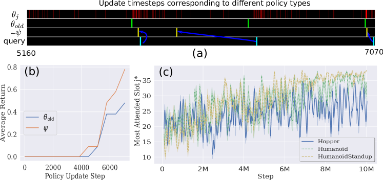
Figure 1: (a) Policy analysis on Unlock. First row (red lines): steps where a policy is added to $\mathcal{M}$, i.e. the steps of $\theta_{j}$. Second row (green lines): steps of old policies $\theta_{old}$. Third row (yellow lines): steps of mostly attended policy, approximating $\psi$. Fourth row (cyan lines): 3 steps of interest where we want to find their attended steps. Blue arrows link a query step and the step that receives highest attention. (b) Quality of $\psi$ vs. $\theta_{old}$. Average return collected by $\psi$ and $\theta_{old}$ at different stages of training. (c) 3 Mujoco tasks. The slot in $\mathcal{M}$ received the highest attention $j^{*}=\mathrm{argmax_{j}}\,f_{\varphi}\left(v_{context}\right)_{j}$ over time.

4.2 Navigation

Here, we validate our method on sparse reward environments using MiniGrid library Chevalier-Boisvert et al. (2018). In particular, we test MCPO and other baselines (same as above) on Unlock and UnlockPickup tasks. In these tasks, the agent navigates through rooms and picks up objects to complete the episode. The agent only receives reward +1 if it can complete the episode successfully. For sample efficiency test, we train all models on Unlock (find key and open the door) and UnlockPickup (find key, open the door and pickup an object), for only 100,000 and 1 million environment steps, respectively. The models use the best conservative hyperparameters found in the previous task (more in Appendix B.3).

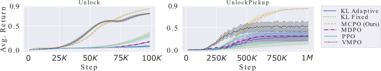
Figure 3: Unlock (left) and UnlockPickup (right)’s learning curves (mean and std. over 10 runs).

Appendix’s Fig. 3 shows the learning curves of examined models on these two tasks. For Unlock task, except for MCPO and VMPO, 100,000 steps seem insufficient for other models to learn useful policies. When trained with 1 million steps on UnlockPickup, the baselines can find better policies, yet still underperform MCPO. Here VMPO shows faster learning progress than MCPO at the beginning, however it fails to converge to the best solution. Our MCPO is the best performer, consistently ending up with average return of 0.9 (90% of episodes finished successfully). To achieve sample-efficiency, MCPO needs to store and search for good policies (rarely found in sparse reward problems), and adhere to it during optimization. MCPO’s success may be attributed to utilizing the virtual policy that has the highest return.

To illustrate how the virtual policy supports MCPO’s performance, we analyze the relationships between the old ($\theta_{old}$), the virtual policy ($\psi$) and the policies stored in $\mathcal{M}$ ($\theta_{j}$) throughout Unlock training. Fig. 1 (a) plots the location of these policies over a truncated period of training (from update step 5160 to 7070). Due to diversity-promoting rule, the steps where policies are added to $\mathcal{M}$ can be uneven (first row-red lines), often distributed right after the locations of the old policy (second row-green lines). We query at $10$-th step behind the old policy (fourth row-cyan lines) to find which policy in $\mathcal{M}$ has the highest attention (third row-yellow lines, linked by blue arrows). As shown in Fig. 1 (a) (second and third row), the attended policy, which mostly resembles $\psi$, can be further or closer to the query step than the old policy depending on the training stage. Since we let the attention network learn to attend to the policy that maximizes the advantage of current mini-batch data, the attended one is not necessarily the old policy.

Model	HalfCheetah	Walker2d	Hopper	Ant	Humanoid	HumanoidStandup
TRPO	2,811±114	3,966±56	3,159±72	2,438±402	4,576±106	145,143±3,702
PPO	4,753±1,614	5,278±594	2,968±1,002	3,421±534	3,375±1,684	155,494±6,663
MDPO	4,774±1,598	4,957±330	3,153±956	3,553±696	1,620±2,145	90,646±5,855
TRGPPO	2,811±114	5,009±391	3,713±275	4,796±837	6,242±1192	162,185±3755
Mean $\psi$	4,942±3,095	5,056±842	3,430±259	4,570±548	353±27	71,308±11,113
MCPO	6,173±595	5,120±588	3,620±252	4673±249	4,848±711	195,404±32,801

Table 2: Mean and std. over 5 runs on 6 Mujoco tasks at 10M environment steps.

The choice of the chosen virtual policy being better than the old policy is shown in Fig. 1 (b) where we collect several checkpoints of virtual and old policies across training and evaluate each of them on 10 testing episodes. Here using $\psi$ to form the second KL constraint is beneficial as the new policy is generally pulled toward a better policy during training. That contributes to the excellent performance of MCPO compared to other single trust-region baselines, especially KL Fixed and Adaptive, which are very close to MCPO in term of objective function style.

4.3 Mujoco

Next, we examine MCPO and some trust-region methods from the literature that are known to have good performance on continuous control problems: TRPO, PPO, MDPO and TRGPPO (an improved version of PPO). To understand the role of the attention network in MCPO, we design a variant of MCPO ($N=40$): Mean $\psi$, which simply constructs $\psi$ by taking average over policy parameters in $\mathcal{M}$. This baseline represents prior heuristic ways of building trust-region from past policies Wang et al. (2016). We pick 6 hard Mujoco tasks and train each model for 10 million environment steps. We report the results of best tuned models in Table 2 (see Appendix B.4 for full results).

The results show that MCPO consistently achieves good performance across 6 tasks, where it outperforms others significantly in HalfCheetah, Hopper, and HumanoidStandup. In other tasks, MCPO is the second best, only slightly earning less score than the best one in Walker2d and Ant. The variant Mean $\psi$ shows reasonable performance for the first 4 tasks, yet almost fails to learn on the last two. Thus, mean virtual policy can perform badly.

To understand the effectiveness of the attention network, we visualize the attention pattern of MCPO on the last two tasks and on Hopper-a task that Mean $\psi$ performs well on. Fig. 1 (c) illustrates that for the first two harder tasks, MCPO gradually learns to favor older policies in $\mathcal{M}$ $(j^{*}>35)$, which puts more restriction on the policy change as the model converges. This strategy seems critical for those tasks as the difference in average return between learned $\psi$ and Mean $\psi$ is huge in these cases. On the other hand, on Hopper, the top attended slots are just above the middle policies in $\mathcal{M}$ $(j^{*}\sim 25)$, which means this task prefers an average restriction. As in most cases, MCPO with big policy memory ($N=40$, more conservativeness) is beneficial. For those tasks where MCPO does not show clear advantage, we speculate that conservative updates are less important.

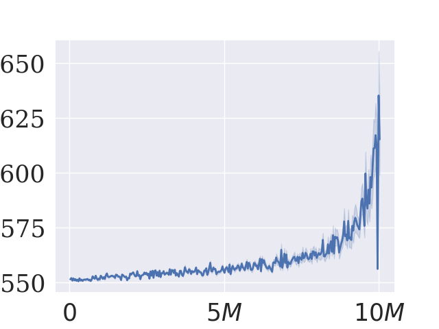
Figure 4: HalfCheetah: Average $\alpha_{t}$ over training time (mean and std. over 3 runs). The training does not use learning rate decay to ensure that $\psi$ and $\theta_{old}$ do not converge to the same policy towards the end of training.

We also visualize $\alpha_{t}$ for HalfCheetah task, and observe an increasing trend across training steps (see Appendix Fig. 4). As the attention network gets trained, the virtual policy becomes better and can complement the old policy when the latter performs worse. Hence, on average, the weight $\alpha_{t}$ tends to be bigger overtime.

4.4 Atari Games

As showcasing the robustness of our method to high-dimensional inputs, we execute an experiment on a subset of Atari games wherein the states are screen images and the policy and value function approximator uses deep convolutional neural networks. We choose 9 typical games (6 were introduced in Mnih et al. (2013) and 3 randomly chosen) and benchmark MCPO against PPO, ACKTR, VMPO and PRGPPO, training all models for only 10 million environment steps. In this experiment, MCPO uses $N=10$ and other baselines’ hyperparameters are selected based on the original papers (see Appendix B.5).

Model	PPO	ACKTR	VMPO	TRGPPO	MCPO
Mean	131.19	195.52	18.20	116.80	229.99
Median	52.85	25.30	13.56	43.24	65.78

Table 3: Average normalized human score over 9 games. The performance of each run is measured by the best checkpoint during training over 10 million frames, averaged over 5 runs.

As seen in Table 3, MCPO is significantly better than other baselines in terms of both mean and median normalized human score. The learning curves of all models are given in Appendix Fig. 5. To confirm MCPO maintains the leading performance with more training iterations, we train competitive models for 40 million frames for the first 6 games (Appendix Fig. 6). The results show that MCPO still outperforms other baselines after 40M frames.

4.5 Ablation Study

Finally, we verify MCPO’s 3 components: virtual policy (in Eq. 3), switching-$\beta$ (Eq. 4) and diversity-promoting rule (Eq. 2). We also confirm the role of choosing the right memory size $N$ and learning to attend to the virtual policy $\psi$. In the task BipedalWalkerHardcore (OpenAI Gym), we train MCPO with different configurations for 50M steps. First, we tune $N$ (5,10 and 40) using the normal MCPO with all components on and find that $N=10$ is the best. Keeping $N=10$, we ablate or replace our component with an alternative and report the findings as follows.

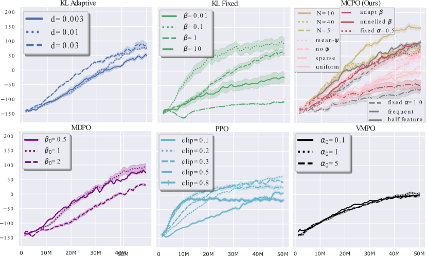
Figure 2: Ablation study on BibedalWalkerHardcore-v3: learning curves (mean and std. over 5 runs) across 50M training steps.

Virtual policy: To show the benefit of pushing the new policy toward the virtual policy, we implement 3 variants of MCPO (N=10) that (i) does not use $\psi$’s KL term in Eq. 3 ($\alpha_{t}=0$), (ii) use a fixed $\alpha_{t}=0.5$ and (iii) only use $\psi$’s KL ($\alpha_{t}=1.0$). All variants underperforms the normal MCPO by a margin of 100 or 50 return. Switching-$\beta$: The results show that compared to the annealed $\beta$ strategy adopted from MDPO and adaptive $\beta$ from PPO-KL, our switching-$\beta$ achieves significantly better results with about 50 and 200 return score higher, respectively. Diversity-promoting writing: We compare our proposal with the vanilla approach that adds a new policy to $\mathcal{M}$ at every update step (frequent writing) and other versions that write to $\mathcal{M}$ every interval of 10 and 100 update steps (uniform and sparse writing). Frequent, uniform and sparse writing all show slow learning progress, and ends up with low rewards. Perhaps, frequently adding policies to $\mathcal{M}$ makes the memory content similar, hastening the removal of older, yet maybe valuable policies. Uniform and sparse writing are better, yet it can still add similar policies to $\mathcal{M}$ and requires additional effort for tuning the writing interval. Learned $\psi$: To benchmark, we try alternatives: (1) using Mean $\psi$ and (2) only using half of the features in $v_{context}$ to generate $\psi$ (Eq. 1). The results confirm that the Mean $\psi$ is not a strong baseline for this task, only reaping moderate rewards. Using less features for the context causes information loss, hinders generations of useful $\psi$, and thus, underperforms the full-feature version by a margin of 50 return. For completeness, we also compare our methods to heavily tuned baselines and confirm that the normal MCPO ($N=10$) is the best performer (see the details in Appendix B.6).

5 Related work

A framework for model-free reinforcement learning with policy gradient is approximate policy iteration (API), which alternates between estimating the advantage of the current policy, and updating the current policy’s parameters to obtain a new policy by maximizing the expected advantage Bertsekas and Tsitsiklis (1995); Sutton et al. (2000). Theoretical studies have shown that constraining policy updates is critical for API Kakade and Langford (2002); Schulman et al. (2015a); Shani et al. (2020); Vieillard et al. (2020b). An early attempt to improve API is Conservative Policy Iteration (CPI), which sets the new policy as a stochastic mixture of previous greedy policies Kakade and Langford (2002); Pirotta et al. (2013); Vieillard et al. (2020a). Our paper differs from these works in three aspects: (1) we do not directly set the new policy to the mixture, rather, we use a mixture of previously found policies (the virtual policy) to define the trust region constraining the new policy via KL regularization; (2) our mixture can consist of more than 2 modes, and thus using multiple mixture weights (attention weights); (3) we use the attention network to learn these weights.

Also motivated by Kakade et al. (2002), TRPO extends the theory to general stochastic policies, rather than just mixture polices, ensuring monotonic improvement by combining maximizing the approximate expected advantage with minimizing the KL divergence between two consecutive policies Schulman et al. (2015a). Arguing that optimizing this way is too conservative and hard to tune, the authors reformulate the objective as a constrained optimization problem to solve it with conjugate gradient and line search. To simplify the implementation of TRPO, Schulman et al. (2017) introduces first-order optimization methods and code-level improvement, which results in PPO–an API method that optimizes a clipped surrogate objective using minibatch updates.

Constrained policy improvement can be seen as Expectation-Maximization algorithms where minimizing the KL-term corresponds to the Expectation step, which can be off-policy Abdolmaleki et al. (2018) or on-policy Song et al. (2019). From the mirror descent perspective, several works also use KL divergence to regularize policy updates Yang et al. (2019); Tomar et al. (2020); Shani et al. (2020). A recent analysis also points out the advantages of using KL term as a regularizer over a hard constraint Lazic et al. (2021). Some other works improve PPO with adaptive clip range Wang et al. (2019) or off-policy data Fakoor et al. (2020). We instead advocate using 2 trust regions and apply our idea to a weaker backbone: PPO-penalty. Our method is also different from Fakoor et al. (2020) as we do not use off-policy data/gradients to update the policy. Overall, our approach shares similarities with them where we also jointly optimize the approximate expected advantage and KL constraint terms for multiple epochs of minibatch updates. However, we propose a novel dynamic virtual policy to construct the second trust region as a supplement to the traditional trust region defined by the old or previous policy.

Prior works have promoted different utilization of memory to assist reinforcement learning. Unlike episodic memory concepts that stores observations across agent’s life Blundell et al. (2016); Le et al. (2021), the memory buffer used in this paper stores the weight parameters of the policy network and attention mechanism is used to query this memory. The proposed memory instead can be viewed as an instance of program memory Le et al. (2019b); Le and Venkatesh (2022). That said, our memory is different from these prior works since our attention is learned through an auxiliary objective that optimizes the quality of the attended policy (program) with novel diversity-promoting writing mechanisms.

6 Discussion

We have presented Memory-Constrained Policy Optimization, a new method to regularize each policy update with two-trust regions with respect to one single old policy and another virtual policy representing multiple past policies. The new policy is encouraged to stay closer to the region surrounding the policy that performs better. The virtual policy is determined online through a learned attention to a memory of past policies. Compared to other trust-region optimizations, MCPO shows better performance in many environments without much hyperparameter tuning.

Limitations

Our method introduces several new components and hyperparameters such as $N$ and $\beta$. Due to compute limit, we have not tuned $\beta$ extensively and thus the reported results may not be the best performance that our model can achieve. Although we find the default values $\beta_{max}=10$, $\beta_{min}=0.01$ work well across all experiments in this paper, we recommend adjustments if users apply our method to novel domains.

Negative Societal Impacts

Our work aims to improve optimization in RL to reduce the sample complexity of RL algorithms. This aim is genuine, and we do not think there are immediate harmful consequences. However, we are aware of potential problems such as unsafe exploration committed by the agent (e.g. causing accidents) in real-world environments (e.g. self-driving cars). Finally, malicious users can misuse our method for unethical purposes, such as training harmful RL agents and robots. This issue is typical for any machine learning algorithm, and we will do our best to prevent it from our end.

Appendix

A Method Details

A.1 The attention network

The attention network is implemented as a feedforward neural network with one hidden layer:

• Input layer: 12 units

• Hidden layer: $N$ units coupled with a dropout layer $p=0.5$

• Output layer: $N$ units, $\mathrm{softmax}$ activation function

$N$ is the capacity of policy memory. The 12 features of the input $v_{context}$ is listed in Table 4.

Now we explain the motivation behind these feature design. From these three policies, we tried to extract all possible information. The information should be cheap to extract and dependent on the current data, so we prefer features extracted from the outputs of these policies (value, entropy, distance, return, etc.). Intuitively, the most important features should be the empirical returns, values associated with each policy and the distances, which gives a good hint of which virtual policy will yield high performance (e.g., a virtual policy that is closer to the policy that obtained high return and low value loss).

A.2 The advantage function

In this paper, we use GAE [18] as the advantage function for all models and experiments

$$\hat{A}_{t} =\frac{1}{N_{actor}}\sum_{i}^{N_{actor}}\sum_{k=0}^{T-t-1}\left(\gamma\lambda\right)^{k}\left(V_{target}-V\left(s_{t+k}^{i}\right)\right)$$

where $\gamma$ is the discounted factor and $N_{actor}$ is the number of actors. $V_{target}=r_{t+k}^{i}+\gamma V\left(s_{t+k+1}^{i}\right)$. Note that Algo. 1 illustrates the procedure for 1 actor. In practice, we use $N_{actor}$ depending on the tasks.

A.3 The objective function

Following [19], our objective function also includes value loss and entropy terms. This is applied to all of the baselines. For example, the complete objective function for MCPO reads

$$L =L^{MCPO}-c_{1}\hat{\mathbb{E}}_{t}\left(V_{\theta}\left(s_{t}\right)-V_{target}\left(s_{t}\right)\right)^{2}$$

$$+c_{2}\hat{\mathbb{E}}_{t}\left[-\log\left(\pi_{\theta}\left(\cdot|s_{t}\right)\right)\right]$$

where $c_{1}$ and $c_{2}$ are value and entropy coefficient hyperparameters, respectively. $V_{\theta}$ is the value network, also parameterized with $\theta$.

B Experimental Details

B.1 Baselines and tasks

All baselines in this paper share the same setting of policy and value networks. Except for TRPO, all other baselines use minibatch training. The only difference is the objective function, which revolves around KL and advantage terms. We train all models with Adam optimizer. We summarize the policy and value network architecture in Table 5.

The baselines ACKTR, PPO, TRPO use available public code (Apache or MIT License). They are Pytorch reimplementation of OpenAI’s stable baselines, which can reproduce the original performance relatively well. For MDPO, we refer to the authors’ source code to reimplement the method. For VMPO, we refer to this open source code to reimplement the method. We implement KL Fixed and KL Adaptive, using objective function defined in Sec. 2.

We use environments from Open AI gyms , which are public and using The MIT License. Mujoco environments use Mujoco software (our license is academic lab). Table 6 lists all the environments.

Dimension	Feature	Meaning
1	$D\left(\theta,\psi_{old}\right)$	“Distance” between $\theta$ and $\psi_{old}$
2	$D\left(\theta_{old},\psi_{old}\right)$	“Distance” between $\theta_{old}$ and $\psi_{old}$
3	$D\left(\theta_{old},\theta\right)$	“Distance” between $\theta_{old}$ and $\theta$
4	$\hat{\mathbb{E}}_{t}\left[R_{t}\left(\psi_{old}\right)\right]$	Approximate expected advantage of $\psi_{old}$
5	$\hat{\mathbb{E}}_{t}\left[R_{t}\left(\theta_{old}\right)\right]$	Approximate expected advantage of $\theta_{old}$
6	$\hat{\mathbb{E}}_{t}\left[R_{t}\left(\theta\right)\right]$	Approximate expected advantage of $\theta$
7	$\hat{\mathbb{E}}_{t}\left[-\log\left(\pi_{\psi_{old}}\left(\cdot|s_{t}\right)\right)\right]$	Approximate entropy of $\psi_{old}$
8	$\hat{\mathbb{E}}_{t}\left[-\log\left(\pi_{\theta_{old}}\left(\cdot|s_{t}\right)\right)\right]$	Approximate entropy of $\theta_{old}$
9	$\hat{\mathbb{E}}_{t}\left[-\log\left(\pi_{\theta}\left(\cdot|s_{t}\right)\right)\right]$	Approximate entropy of $\theta$
10	$\hat{\mathbb{E}}_{t}\left(V_{\psi_{old}}\left(s_{t}\right)-V_{target}\left(s_{t}\right)\right)^{2}$	Value loss of $\psi_{old}$
11	$\hat{\mathbb{E}}_{t}\left(V_{\theta_{old}}\left(s_{t}\right)-V_{target}\left(s_{t}\right)\right)^{2}$	Value loss of $\theta_{old}$
12	$\hat{\mathbb{E}}_{t}\left(V_{\theta}\left(s_{t}\right)-V_{target}\left(s_{t}\right)\right)^{2}$	Value loss of $\theta$

Table 4: Features of the context vector.

Input type	Policy/Value networks
Vector	2-layer feedforward
	net (tanh, h=64)
Image	3-layer ReLU CNN with
	kernels $\left\{32/8/4,64/4/2,32/3/1\right\}$+2-layer
	feedforward net (ReLU, h=512)

Table 5: Network architecture shared across baselines.

Tasks	Continuous	Gym
	action	category
Pendulum-v0	$\mathit{\mathtt{X}}$	Classical
LunarLander-v2		Box2d
BipedalWalker-v3	$\checked$
Unlock-v0	$\mathit{\mathtt{X}}$	MiniGrid
UnlockPickup-v0
MuJoCo tasks (v2): HalfCheetah	$\checked$	MuJoCo
Walker2d, Hopper, Ant
Humanoid, HumanoidStandup
Atari games (NoFramskip-v4):	$\mathit{\mathtt{X}}$	Atari
Beamrider, Breakout
Enduro, Gopher
Seaquest, SpaceInvaders
BipedalWalkerHardcore-v3	$\checked$	Box2d

Table 6: Tasks used in the paper.

B.2 Details on Classical Control

Model	Pendulum	LunarLander	BWalker
	1M	1M	5M
KL Adaptive ($d_{targ}=0.003$)	-407.74±484.16	238.30±34.07	206.99±5.34
KL Adaptive ($d_{targ}=0.01$)	-147.52±9.90	254.26±19.43	247.70±14.16
KL Adaptive ($d_{targ}=0.03$)	-601.09±273.18	246.93±12.57	259.80±6.33
KL Fixed ($\beta=0.01$)	-1051.14±158.81	247.61±19.79	221.55±38.64
KL Fixed ($\beta=0.1$)	-464.29±426.27	256.75±20.53	263.56±10.04
KL Fixed ($\beta=1$)	-136.40±4.49	192.62±32.97	215.13±13.29
PPO (clip $\epsilon=0.1$)	-282.20±243.42	242.98±13.50	205.07±19.13
PPO (clip $\epsilon=0.2$)	-514.28±385.34	256.88±20.33	253.58±7.49
PPO (clip $\epsilon=0.3$)	-591.31±229.32	259.93±22.52	260.51±17.86
MDPO ($\beta_{0}=0.5$)	-136.45±8.21	247.96±4.74	251.18±29.10
MDPO ($\beta_{0}=1$)	-139.14±10.32	207.96±43.86	245.27±10.47
MDPO ($\beta_{0}=2$)	-135.52±5.28	227.76±16.96	226.80±15.67
VMPO ($\alpha_{0}=0.1$)	-144.51±7.04	201.87±29.48	236.57±10.62
VMPO ($\alpha_{0}=1$)	-139.50±5.54	212.85±43.35	238.82±11.11
VMPO ($\alpha_{0}=5$)	-296.48±213.06	222.13±35.55	164.40±40.36
MCPO ($N=5$)	-133.42±4.53	262.23±12.47	265.80±5.55
MCPO ($N=10$)	-146.88±3.78	263.04±11.48	266.26±8.87
MCPO ($N=40$)	-135.57±5.22	267.19±13.42	249.51±12.75

Table 7: Mean and std. over 5 runs on classical control tasks (with number of training environment steps). Bold denotes the best mean. Underline denotes good results (if exist), statistically indifferent from the best in terms of Cohen effect size less than 0.5.

For these tasks, all models share hyperparameters listed in Table 8. Besides, each method has its own set of additional hyperparameters. For example, PPO, KL Fixed and KL Adaptive have $\epsilon$, $\beta$ and $d_{targ}$, respectively. These hyperparameters directly control the conservativeness of the policy update for each method. For MDPO, $\beta$ is automatically reduced overtime through an annealing process from 1 to 0 and thus should not be considered as a hyperparameter. However, we can still control the conservativeness if $\beta$ is annealed from a different value $\beta_{0}$ rather 1. We realize that tuning $\beta_{0}$ helped MDPO (Table 7). We quickly tried with several values $\beta_{0}$ ranging from 0.01 to 10 on Pendulum, and realize that only $\beta_{0}\in\left\{0.5,1,2\right\}$ gave reasonable results. Thus, we only tuned MDPO with these $\beta_{0}$ in other tasks. For VMPO there are many other hyperparameters such as $\eta_{0}$, $\alpha_{0}$, $\epsilon_{\eta}$ and $\epsilon_{\alpha}$. Due to limited compute, we do not tune all of them. Rather, we only tune $\alpha_{0}$-the initial value of the Lagrange multiplier that scale the KL term in the objective function. We refer to the paper’s and the code repository’s default values of $\alpha_{0}$ to determine possible values $\alpha_{0}\in\left\{0.1,1,5\right\}$. For our MCPO, we can tune several hyperparameters such as $N$, $\beta_{min}$, and $\beta_{max}$. However, for simplicity, we only tune $N\in\left\{5,10,40\right\}$ and fix $\beta_{min}=0.01$ and $\beta_{max}=10$.

On our machines using 1 GPU Tesla V100-SXM2, we measure the running time of MCPO with different $N$ compared to PPO on Pendulum task, which is reported in Table 9. As $N$ increases, the running speed of MCPO decreases. For this reason, we do not test with $N>40$. However, we realize that with $N=5$ or $N=10$, MCPO only runs slightly slower than PPO. We also realize that the speed gap is even reduced when we increase the number of actors $N_{actor}$ as in other experiments. In terms of memory usage, maintaining a policy memory will definitely cost more. However, as our policy, value and attention networks are very simple. The maximum storage even for $N=40$ is less than 5GB.

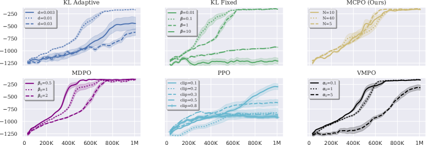
Figure 7: Pendulum-v0: learning curves (mean and std. over 5 runs) across 1M training steps.

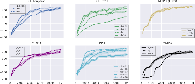
Figure 8: LunarLander-v2: learning curves (mean and std. over 5 runs) across 5M training steps.

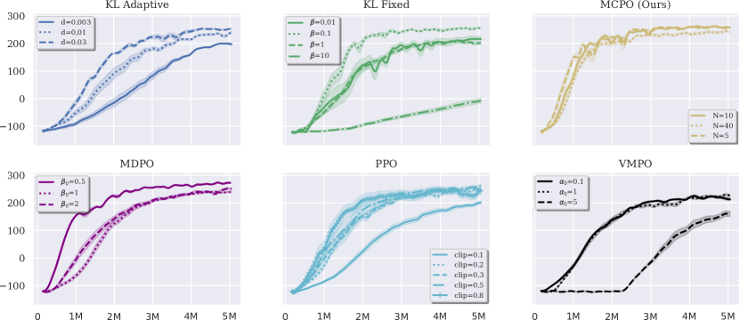
Figure 9: BipedalWalker-v3: learning curves (mean and std. over 5 runs) across 1M training steps.

In addition to the configurations reported in Table 1, for KL Fixed and PPO, we also tested with extreme values $\beta=10$ and $\epsilon\in\left\{0.5,0.8\right\}$. Figs. 7, 8 and 9 visualize the learning curves of all configurations for all models.

Hyperparameter	Pendulum	LunarLander	BipedalWalker	MiniGrid	BipedalWaker
					Hardcore
Horizon $T$	2048	2048	2048	2048	2048
Adam step size	$3\times 10^{-4}$	$3\times 10^{-4}$	$3\times 10^{-4}$	$3\times 10^{-4}$	$3\times 10^{-4}$
Num. epochs $K$	10	10	10	10	10
Minibatch size $B$	64	64	64	64	64
Discount $\gamma$	0.99	0.99	0.99	0.99	0.99
GAE $\lambda$	0.95	0.95	0.95	0.95	0.95
Num. actors $N_{actor}$	4	4	32	4	128
Value coefficient $c_{1}$	0.5	0.5	0.5	0.5	0.5
Entropy coefficient $c_{2}$	0	0	0	0	0

Table 8: Network architecture shared across baselines on Pendulum, LunarLander, BipedalWalker, MiniGrid and BipedalWaker Hardcore

Model	Speed (env. steps/s)
MCPO (N=5)	1,170
MCPO (N=10)	927
MCPO (N=40)	560
PPO	1,250

Table 9: Computing cost of MCPO and PPO on Pendulum.

B.3 Details on MiniGrid Navigation

Based on the results from the above tasks, we pick the best signature hyperparameters for the models to use in this task as in Table 10. In particular, for each model, we rank the hyperparameters per task (higher rank is better), and choose the one that has the maximum total rank. For hyperparameters that share the same total rank, we prefer the middle value. The other hyperparameters for this task is listed in Table 8.

Model	Chosen hyperparameter
KL Adaptive	$d_{targ}=0.01$
KL Fixed	$\beta=0.1$
PPO	$\epsilon=0.2$
MDPO	$\beta_{0}=0.5$
VMPO	$\alpha_{0}=1$
MCPO	$N=10$

Table 10: Signature hyperparameters used in MiniGrid tasks.

B.4 Details on Mujoco

For shared hyperparameters, we use the values suggested in the PPO’s paper, except for the number of actors, which we increase to $16$ for faster training as our models are trained for 10M environment steps (see Table 11).

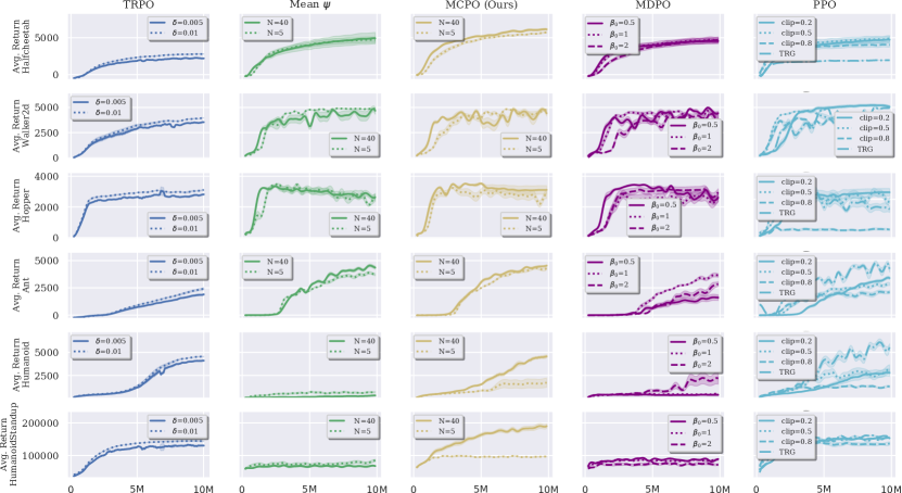
Figure 10: Mujoco: learning curves (mean and std. over 5 runs) across 10M training steps.

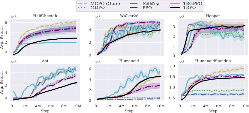
Figure 11: Mujoco: learning curves (mean and std. over 5 runs) across 10M training steps.

For the signature hyperparameter of each method, we select some of the reasonable values. For PPO, the authors already examined with $\epsilon\in\left\{0.1,0.2,0.3\right\}$ on the same task and found 0.2 the best. This is somehow backed up in our previous experiments where we did not see major difference in performance between these values. Hence, seeking for other $\epsilon$ rather than the optimal $\epsilon=0.2$, we ran our PPO implementation with $\epsilon\in\left\{0.2,0.5,0.8\right\}$. For TRPO, the authors only used the KL radius threshold $\delta=0.01$, which may be already the optimal hyperparameter. Hence, we only tried $\delta\in\left\{0.005,0.01\right\}$. The results showed that $\delta=0.005$ always performed worse. For MCPO and Mean $\psi$, we only ran with extreme $N\in\left\{5,40\right\}$. For MDPO, we still tested with $\beta_{0}\in\left\{0.5,1,2\right\}$. Full learning curves with different hyperparameter are reported in Fig. 10. Learning curves including TRGPPO are reported in Fig. 11

Hyperparameter	Mujoco	Atari
Horizon $T$	2048	128
Adam step size	$3\times 10^{-4}$	$2.5\times 10^{-4}$
Num. epochs $K$	10	4
Minibatch size $B$	32	32
Discount $\gamma$	0.99	0.99
GAE $\lambda$	0.95	0.95
Num. actors $N_{actor}$	16	32
Value coefficient $c_{1}$	0.5	1.0
Entropy coefficient $c_{2}$	0	0.01

Table 11: Network architecture shared across baselines on Mujoco and Atari

B.5 Details on Atari

For shared hyperparameters, we use the values suggested in the PPO’s paper, except for the number of actors, which we increase to $32$ for faster training (see Table 11). For the signature hyperparameter of the baselines, we used the recommended value in the original papers. For MCPO, we use $N=10$ to balance between running time and performance. Table 12 shows the values of these hyperparameters.

Model	Chosen hyperparameter
PPO	$\epsilon=0.2$
ACKTR	$\delta=0.01$
VMPO	$\alpha_{0}=5$
MCPO	$N=10$

Table 12: Signature hyperparameters used in Atari tasks.

We also report the average normalized human score (mean and median) of the models over 6 games in Table 3. As seen, MCPO is significantly better than other baselines in terms of both mean and median normalized human score. We also report full learning curves of models and normalized human score including TRGPPO in 9 games in Fig. 5 and Table 3, respectively.

Fig. 5 visualizes the learning curves of the models. Regardless of our regular tuning, VMPO performs poorly, indicating that this method is unsuitable or needs extensive tuning to work for low-sample training regime. ACKTR, works extremely well on certain games (Breakout and Seaquest), but shows mediocre results on others (Enduro, BeamRider), overall underperforming MCPO. PPO is always similar or inferior to MCPO on this testbed. Our MCPO always demonstrates competitive results, outperforming all other models in 4 games, especially on Enduro and Gopher, and showing comparable results with that of the best model in the other 2 games.

To verify whether MCPO can maintain its performance over longer training, we examine Atari training for 40 million frames. As shown in Fig. 6, MCPO is still the best performer in this training regime.

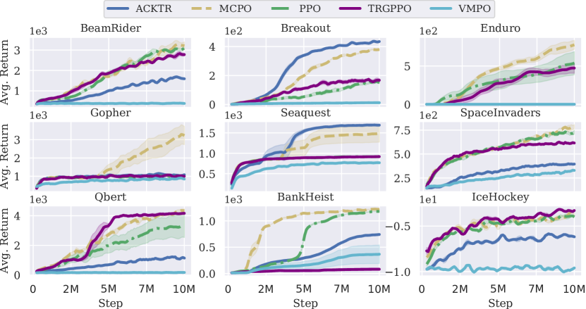
Figure 5: Atari games: learning curves (mean and std. over 5 runs) across 10M training steps.

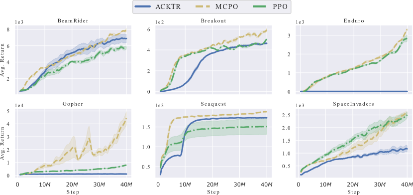
Figure 6: Atari games: learning curves (mean and std. over 5 runs) across 40M training steps.

B.6 Details on ablation study

In this section, we give more details on the ablated baselines. Unless state otherwise, the baseline use $N=10$.

• No $\psi$ We only changed the objective to

  $$L_{1}\left(\theta\right) =\hat{\mathbb{E}}_{t}\left[\tau_{t}\left(\theta\right)\hat{A}_{t}\right]$$

  $$-\beta\hat{\mathbb{E}}_{t}\left[KL\left[\pi_{\theta_{old}}\left(\cdot|s_{t}\right),\pi_{\theta}\left(\cdot|s_{t}\right)\right]\right]$$ (7)

  where $\beta$ is still determined by the $\beta$-switching rule. This baseline corresponds to setting $\alpha=0$

• Fixed $\alpha=0.5$ We manually set $\alpha=0.5$ across training. This baseline uses both old and virtual policy’s trust regions but with fixed balanced coefficient.

• Fixed $\alpha=1.0$ We manually set $\alpha=1.0$ across training. This baseline only uses virtual policy’s trust region.

• Annealed $\beta$ We determine the $\beta$ in Eq. 3 by MDPO’s annealing rule, a.k.a, $\beta_{i}=1.0-\frac{i}{T_{total}}$ where $T_{total}$ is the total number of training policy update steps and $i$ is the current update step. We did not test with other rules such as fixed or adaptive $\beta$ as we realize that MDPO is often better than KL Fixed and KL Adaptive in our experiments, indicating that the annealed $\beta$ is a stronger baseline.

• Adaptive $\beta$ We adopt adaptive $\beta$, determined by the rule introduced in PPO paper (adaptive KL) with $d_{targ}=0.03$.

• Frequent writing We add a new policy to $\mathcal{M}$ at every policy update step.

• Uniform writing Inspired by the uniform writing mechanism in Memory-Augmented Neural Networks [9], we add a new policy to $\mathcal{M}$ at every interval of 10 update steps. The interval size could be tuned to get better results but it would require additional effort, so we preferred our diversity-promoting writing over this one.

• Sparse writing Uniform writing with interval of 100 update steps.

• Mean $\psi$ The virtual policy is determined as

$$\psi=\sum_{j}^{\left|\mathcal{M}\right|}\theta_{j}$$ (8)

• Half feature We only use features from 1 to 6 listed in Table 4.

The other baselines including KL Adaptive, KL Fixed, MDPO, PPO, and VMPO are the same as in B.2. The full learning curves of all models with different hyperparameters are plotted in Fig. 2.

C Theoretical analysis of MCPO

In this section, we explain the design of our objective function $L_{1}$ and $L_{2}$. We want to emphasize that the two trust regions (corresponding to $\theta_{old}$ and $\psi$) are both important for MCPO’s convergence. Eq. 3 needs to include the old policy’s trust region because, in theory, constraining policy updates using the last sampling policy’s trust region guarantees monotonic improvement [17]. However, in practice, the old policy can be suboptimal and may not induce much improvement. This motivates us to employ an additional trust region to regulate the update in case the old policy’s trust region is bad. In doing so, we still want to maintain the theoretical property of trust-region update while enabling a more robust optimization that works well even when the ideal setting for theoretical assurance does not hold.

It should be noted that constraining with a policy different from the sampling one would break the monotonic improvement property of trust-region update. Fortunately, our theory proves that using the two trust regions as defined in our paper helps maintain the monotonic improvement property. This is an important result since if you use an arbitrary virtual policy to form the second trust region (unlike the one we suggest in this paper), the property may not hold.

Similar to [17], we can construct a theoretically guaranteed version of our practical objective functions that ensures monotonic policy improvement.

First, we explain the design of $L_{1}$ by recasting $L_{1}$ as

$$L_{1\theta_{old}}\left(\theta\right) =L_{\theta_{old}}\left(\theta\right)$$

$$-C_{1}D_{KL}^{max}\left(\theta_{old},\theta\right)$$

$$-C_{2}D_{KL}^{max}\left(\psi,\theta\right)$$

where $L_{\theta_{old}}\left(\theta\right)=\eta\left(\pi_{\theta_{old}}\right)+\sum_{s}\rho_{\pi_{\theta_{old}}}\left(s\right)\sum_{a}\pi_{\theta}\left(a|s\right)A_{\pi_{\theta_{old}}}\left(s,a\right)$–the local approximation to the expected discounted return $\eta\left(\theta\right)$, $D_{KL}^{max}\left(a,b\right)=\max_{s}KL\left[\pi_{a}\left(\cdot|s\right),\pi_{b}\left(\cdot|s\right)\right]$, $C_{1}=\frac{4\max_{s,a}\left|A_{\pi}\left(s,a\right)\right|\gamma}{\left(1-\gamma\right)^{2}}$ and $C_{2}>0$. Here, $\rho_{\pi_{\theta_{old}}}$ is the (unnormalized) discounted visitation frequencies induced by the policy $\pi_{\theta_{old}}$.

As the KL is non-negative, $L_{1\theta_{old}}\left(\theta\right)\leq L_{\theta_{old}}\left(\theta\right)-C_{1}D_{KL}^{max}\left(\theta_{old},\theta\right)$. According to [17], the RHS is a lower bound on $\eta\left(\theta\right)$, so $L_{1}$ is also a lower bound on $\eta\left(\theta\right)$ and thus, it is reasonable to maximize the practical $L_{1}$, which is an approximation of $L_{1\theta_{old}}$.

Next, we show that by optimizing both $L_{1}$ and $L_{2}$, we can interpret our algorithm as a monotonic policy improvement procedure. As such, we need to reformulate $L_{2}$ as

$$L_{2\theta_{old}}\left(\psi\right)=L_{\theta_{old}}\left(\psi\right)-C_{1}D_{KL}^{max}\left(\theta_{old},\psi\right)$$

Note that compared to the practical $L_{2}$ (as defined in the main paper on page 5), we have introduced here an additional $KL$ term, which means we need to find $\psi$ that is close to $\theta_{old}$ and maximizes the approximate advantage $L_{\theta_{old}}\left(\psi\right)$. As we maximize $L_{2\theta_{old}}\left(\psi\right)$, the maximizer $\psi$ satisfies

$$L_{2\theta_{old}}\left(\psi\right)\geq L_{2\theta_{old}}\left(\theta_{old}\right)=L_{\theta_{old}}\left(\theta_{old}\right)$$

We also have

$$\eta\left(\theta\right) \geq L_{1\theta_{old}}\left(\theta\right)$$ (9)

$$\eta\left(\theta_{old}\right) =L_{\theta_{old}}\left(\theta_{old}\right)\leq L_{2\theta_{old}}\left(\psi\right)$$

$$=L_{\theta_{old}}\left(\psi\right)-C_{1}D_{KL}^{max}\left(\theta_{old},\psi\right)$$

$$=L_{1\theta_{old}}\left(\psi\right)$$ (10)

Subtracting both sides of Eq. 10 from Eq. 9 yields

$$\eta\left(\theta\right)-\eta\left(\theta_{old}\right)\geq L_{1\theta_{old}}\left(\theta\right)-L_{1\theta_{old}}\left(\psi\right)$$

Thus by maximizing $L_{1\theta_{old}}\left(\theta\right)$, we guarantee that the true objective $\eta\left(\theta\right)$ is non-decreasing.

Although the theory suggests that the optimal $L_{2}$ could be $L_{2}^{*}=\hat{\mathbb{E}}_{t}\left[R_{t}\left(\psi_{\varphi}\right)-C_{1}KL\left[\pi_{\theta_{old}}\left(\cdot|s_{t}\right),\pi_{\psi}\left(\cdot|s_{t}\right)\right]\right]$, it would require additional tuning of $C_{1}$. More importantly, optimizing an objective in form of $L_{2}^{*}$ needs a very small step size, and could converge slowly. Hence, we simply discard the KL term and only optimize $L_{2}=\hat{\mathbb{E}}_{t}\left[R_{t}\left(\psi_{\varphi}\right)\right]$ instead. Empirical results show that using this simplification, MCPO’s learning curves still generally improve monotonically over training time.

References

- Abdolmaleki et al. [2018] Abbas Abdolmaleki, Jost Tobias Springenberg, Yuval Tassa, Remi Munos, Nicolas Heess, and Martin Riedmiller. Maximum a posteriori policy optimisation. In International Conference on Learning Representations, 2018.
- Bertsekas and Tsitsiklis [1995] Dimitri P Bertsekas and John N Tsitsiklis. Neuro-dynamic programming: an overview. In Proceedings of 1995 34th IEEE conference on decision and control, volume 1, pages 560–564. IEEE, 1995.
- Blundell et al. [2016] Charles Blundell, Benigno Uria, Alexander Pritzel, Yazhe Li, Avraham Ruderman, Joel Z Leibo, Jack Rae, Daan Wierstra, and Demis Hassabis. Model-free episodic control. arXiv preprint arXiv:1606.04460, 2016.
- Chevalier-Boisvert et al. [2018] Maxime Chevalier-Boisvert, Lucas Willems, and Suman Pal. Minimalistic gridworld environment for openai gym. https://github.com/maximecb/gym-minigrid, 2018.
- Fakoor et al. [2020] Rasool Fakoor, Pratik Chaudhari, and Alexander J Smola. P3o: Policy-on policy-off policy optimization. In Uncertainty in Artificial Intelligence, pages 1017–1027. PMLR, 2020.
- Kakade and Langford [2002] S. Kakade and J. Langford. Approximately optimal approximate reinforcement learning. In ICML, 2002.
- Lazic et al. [2021] Nevena Lazic, Botao Hao, Yasin Abbasi-Yadkori, Dale Schuurmans, and Csaba Szepesvari. Optimization issues in kl-constrained approximate policy iteration. arXiv preprint arXiv:2102.06234, 2021.
- Le and Venkatesh [2022] Hung Le and Svetha Venkatesh. Neurocoder: General-purpose computation using stored neural programs. In Proceedings of the 39th International Conference on Machine Learning, 2022.
- Le et al. [2019a] Hung Le, Truyen Tran, and Svetha Venkatesh. Learning to remember more with less memorization. arXiv preprint arXiv:1901.01347, 2019a.
- Le et al. [2019b] Hung Le, Truyen Tran, and Svetha Venkatesh. Neural stored-program memory. In International Conference on Learning Representations, 2019b.
- Le et al. [2021] Hung Le, Thommen Karimpanal George, Majid Abdolshah, Truyen Tran, and Svetha Venkatesh. Model-based episodic memory induces dynamic hybrid controls. In A. Beygelzimer, Y. Dauphin, P. Liang, and J. Wortman Vaughan, editors, Advances in Neural Information Processing Systems, 2021. URL https://openreview.net/forum?id=Z9Kpr38Kx_.
- Lillicrap et al. [2016] Timothy P Lillicrap, Jonathan J Hunt, Alexander Pritzel, Nicolas Heess, Tom Erez, Yuval Tassa, David Silver, and Daan Wierstra. Continuous control with deep reinforcement learning. In ICLR (Poster), 2016.
- Mnih et al. [2013] Volodymyr Mnih, Koray Kavukcuoglu, David Silver, Alex Graves, Ioannis Antonoglou, Daan Wierstra, and Martin Riedmiller. Playing atari with deep reinforcement learning. arXiv preprint arXiv:1312.5602, 2013.
- Mnih et al. [2015] Volodymyr Mnih, Koray Kavukcuoglu, David Silver, Andrei A Rusu, Joel Veness, Marc G Bellemare, Alex Graves, Martin Riedmiller, Andreas K Fidjeland, Georg Ostrovski, et al. Human-level control through deep reinforcement learning. nature, 518(7540):529–533, 2015.
- Mnih et al. [2016] Volodymyr Mnih, Adria Puigdomenech Badia, Mehdi Mirza, Alex Graves, Timothy Lillicrap, Tim Harley, David Silver, and Koray Kavukcuoglu. Asynchronous methods for deep reinforcement learning. In International conference on machine learning, pages 1928–1937. PMLR, 2016.
- Pirotta et al. [2013] Matteo Pirotta, Marcello Restelli, Alessio Pecorino, and Daniele Calandriello. Safe policy iteration. In International Conference on Machine Learning, pages 307–315. PMLR, 2013.
- Schulman et al. [2015a] John Schulman, Sergey Levine, Pieter Abbeel, Michael Jordan, and Philipp Moritz. Trust region policy optimization. In International conference on machine learning, pages 1889–1897. PMLR, 2015a.
- Schulman et al. [2015b] John Schulman, Philipp Moritz, Sergey Levine, Michael Jordan, and Pieter Abbeel. High-dimensional continuous control using generalized advantage estimation. arXiv preprint arXiv:1506.02438, 2015b.
- Schulman et al. [2017] John Schulman, Filip Wolski, Prafulla Dhariwal, Alec Radford, and Oleg Klimov. Proximal policy optimization algorithms. arXiv preprint arXiv:1707.06347, 2017.
- Shani et al. [2020] Lior Shani, Yonathan Efroni, and Shie Mannor. Adaptive trust region policy optimization: Global convergence and faster rates for regularized mdps. In Proceedings of the AAAI Conference on Artificial Intelligence, volume 34, pages 5668–5675, 2020.
- Silver et al. [2017] David Silver, Julian Schrittwieser, Karen Simonyan, Ioannis Antonoglou, Aja Huang, Arthur Guez, Thomas Hubert, Lucas Baker, Matthew Lai, Adrian Bolton, et al. Mastering the game of go without human knowledge. nature, 550(7676):354–359, 2017.
- Song et al. [2019] H Francis Song, Abbas Abdolmaleki, Jost Tobias Springenberg, Aidan Clark, Hubert Soyer, Jack W Rae, Seb Noury, Arun Ahuja, Siqi Liu, Dhruva Tirumala, et al. V-mpo: On-policy maximum a posteriori policy optimization for discrete and continuous control. In International Conference on Learning Representations, 2019.
- Sutton et al. [2000] Richard S Sutton, David A McAllester, Satinder P Singh, and Yishay Mansour. Policy gradient methods for reinforcement learning with function approximation. In Advances in neural information processing systems, pages 1057–1063, 2000.
- Tomar et al. [2020] Manan Tomar, Lior Shani, Yonathan Efroni, and Mohammad Ghavamzadeh. Mirror descent policy optimization. arXiv preprint arXiv:2005.09814, 2020.
- Vieillard et al. [2020a] Nino Vieillard, Olivier Pietquin, and Matthieu Geist. Deep conservative policy iteration. In Proceedings of the AAAI Conference on Artificial Intelligence, volume 34, pages 6070–6077, 2020a.
- Vieillard et al. [2020b] Nino Vieillard, Bruno Scherrer, Olivier Pietquin, and Matthieu Geist. Momentum in reinforcement learning. In International Conference on Artificial Intelligence and Statistics, pages 2529–2538. PMLR, 2020b.
- Wang et al. [2019] Yuhui Wang, Hao He, Xiaoyang Tan, and Yaozhong Gan. Trust region-guided proximal policy optimization. Advances in Neural Information Processing Systems, 32:626–636, 2019.
- Wang et al. [2016] Ziyu Wang, Victor Bapst, Nicolas Heess, Volodymyr Mnih, Remi Munos, Koray Kavukcuoglu, and Nando de Freitas. Sample efficient actor-critic with experience replay. arXiv preprint arXiv:1611.01224, 2016.
- Watkins and Dayan [1992] Christopher JCH Watkins and Peter Dayan. Q-learning. Machine learning, 8(3-4):279–292, 1992.
- Wu et al. [2017] Yuhuai Wu, Elman Mansimov, Shun Liao, Roger Grosse, and Jimmy Ba. Scalable trust-region method for deep reinforcement learning using kronecker-factored approximation. In Proceedings of the 31st International Conference on Neural Information Processing Systems, pages 5285–5294, 2017.
- Yang et al. [2019] Long Yang, Gang Zheng, Haotian Zhang, Yu Zhang, Qian Zheng, Jun Wen, and Gang Pan. Policy optimization with stochastic mirror descent. arXiv preprint arXiv:1906.10462, 2019.