Heavy-Ball-Based Hard Thresholding Algorithms for Sparse Signal Recovery

Abstract. The hard thresholding technique plays a vital role in the development of algorithms for sparse signal recovery. By merging this technique and heavy-ball acceleration method which is a multi-step extension of the traditional gradient descent method, we propose the so-called heavy-ball-based hard thresholding (HBHT) and heavy-ball-based hard thresholding pursuit (HBHTP) algorithms for signal recovery. It turns out that the HBHT and HBHTP can successfully recover a $k$-sparse signal if the restricted isometry constant of the measurement matrix satisfies $\delta_{3k}<0.618$ and $\delta_{3k}<0.577,$ respectively. The guaranteed success of HBHT and HBHTP is also shown under the conditions $\delta_{2k}<0.356$ and $\delta_{2k}<0.377,$ respectively. Moreover, the finite convergence and stability of the two algorithms are also established in this paper. Simulations on random problem instances are performed to compare the performance of the proposed algorithms and several existing ones. Empirical results indicate that the HBHTP performs very comparably to a few existing algorithms and it takes less average time to achieve the signal recovery than these existing methods.

Key words: Compressed sensing, Heavy-ball method, Sparse signal recovery, Hard thresholding algorithm, Restricted isometry property, Phase transition.

1 Introduction

In compressed sensing scenarios, one needs to recover a sparse signal $x\in\mathbb{R}^{n}$ from linear measurements $y:=Ax+\nu$, where $\nu\in\mathbb{R}^{m}$ are measurement errors and $A$ is a known $m\times n$ measurement matrix with $m\ll n.$ When $\nu=0$, the measurements $y$ are accurate. To recover the signal $x$ in such an environment, one may consider the optimization model

$$\underset{z}{\min}\{{\left\lVert y-Az\right\rVert}_{2}^{2}:\left\lVert z\right\rVert_{0}\leq k\},$$ (1)

where $k$ (a given integer number) is an estimate of the sparsity level of $x,$ and $\left\lVert z\right\rVert_{0}$ denotes the number of nonzero entries of $z\in\mathbb{R}^{n}.$ In this paper, a vector $z$ is said to be $k$-sparse if $\left\lVert z\right\rVert_{0}\leq k$. It is well known that when $x$ is $k$-sparse and $A$ satisfies certain assumptions, $x$ will be the unique $k$-sparse solution to the problem (1) (see, e.g., [15, 17, 37]). Thus the recovery of $x$ often amounts to solving the problem (1), and the algorithms for such a prpoblem are usually called compressed sensing algorithms or, in more general, sparse optimization algorithms.

Let us first briefly review the thresholding algorithms for sparse signal recovery. The thresholding technique was introduced by Donoho and Johnstone [13]. At present, there are three main classes of thresholding algorithms: hard thresholding [2, 3, 4, 5, 6, 8, 16, 22, 23], soft thresholding [10, 12, 14], and optimal thresholding [26, 38, 40]. A huge amount of work has been carried out for the class of hard thresholding algorithms. For instance, the iterative hard thresholding (IHT) was early studied in [4], which is a combination of the gradient descent and hard thresholding technique. The IHT admits a few modifications including the gradient descent with sparsification (GDS) [18] and the normalized iterative hard thresholding with a fixed or adaptive steplength [3, 6]. In addition, combining IHT [4, 6, 18] and orthogonal projection immediately leads to the hard thresholding pursuit (HTP) in [16]. The thresholding methods combined with Nesterov’s acceleration technique were also studied (e.g., [8, 22, 23]). Recently, it was pointed out in [38] that performing hard thresholding is usually independent of the reduction of the residual $\|y-Az\|_{2}^{2}$ and thus the so-called optimal $k$-thresholding operator was proposed in [38, 40]. Nevertheless, the optimal $k$-thresholding algorithm need to solve a quadratic convex optimization problem at every iteration which requires more computational time than the traditional hard thresholding methods.

The aim of this paper is to use the heavy ball method to accelerate the hard thresholding algorithms without increasing its computational complexity. Recall that the search direction at the iterate $x^{p}$ in IHT and HTP is given by $A^{T}(y-Ax^{p})$, which is the negative gradient of the residual at $x^{p}.$ With the aid of the momentum term $x^{p}-x^{p-1}$, the search direction can be modified to

$$d^{p}=\alpha A^{T}(y-Ax^{p})+\beta(x^{p}-x^{p-1})$$ (2)

with two parameters $\alpha>0$ and $\beta\geq 0.$ This is the two-step heavy-ball method proposed for optimization problems by Polyak [29]. It has been shown that a fast local convergence of this method for optimization problems can be achieved provided that the parameters are properly chosen, and that the method can work even when the Hessian matrix of the objective function is ill-posed (see, e.g., Chapter 3 in [30]). The global convergence of the heavy ball method has also been discussed in the literature [19, 20, 24, 36]. This method is widely used in such fields as distributed optimization [20, 36], variational inequality [21], wireless network [25], nonconvex optimization [28, 32], deep neural network [33], and image restoration [35]. For instance, it was found in [32] that the heavy ball momentum plays an important role in driving the iterates away from the saddle points of nonconvex optimization problems; It was also used in [35] to accelerate the Richardson-Lucy algorithm in image deconvolution without causing a remarkable increase of iteration complexity; Xin and Khan [36] observed that the distributed heavy ball method achieves a global $R-$linear rate for distributed optimization, and the momentum term can dramatically improves the convergence of the algorithm for ill-conditioned objective functions. These and other applications indicate that the heavy-ball method does admit certain advantage in enhancing the efficiency of an iterative method for optimization problems and may outperform the extra-point method and Nesterov acceleration method.

Motivated by the numerical advantage of heavy ball acceleration technique, we propose the heavy-ball-based hard thresholding (HBHT) and heavy-ball-based hard thresholding pursuit (HBHTP) algorithms for the recovery problem (1). The guaranteed performance of the two algorithms are shown under the assumption of restricted isometry property (RIP), which was originally introduced by Candès and Tao [7] and has now become a standard tool for the analysis of various compressed sensing algorithms. It is well known that the success of IHT for $k$-sparse signal recovery can be guaranteed under the RIP condition $\delta_{3k}<(\sqrt{5}-1)/2\approx 0.618$ (see [39]) and that of HTP can be guaranteed under $\delta_{3k}<1/\sqrt{3}\approx 0.577$ (see [16]). Under the same condition and a proper choice of algorithmic parameters, we establish the guaranteed-performance results for the two algorithms HBHT and HBHTP. Roughly speaking, we show that the HBHT is convergent under the condition $\delta_{3k}<(\sqrt{5}-1)/2$ and that HBHTP is convergent under the condition $\delta_{3k}<1/\sqrt{3}.$ By using an analysis method in [40], we further prove that the condition for theoretical performance of the two algorithms can be established in term of $\delta_{2k}$ as well. Specifically, the guaranteed success of HBHT and HBHTP can be ensured if $\delta_{2k}<(\sqrt{5}-1)/(2\sqrt{3})\approx 0.356$ and $\delta_{2k}<1/\sqrt{7}\approx 0.377$, respectively. Moreover, the finite convergence and recovery stability of the two methods are also shown in this paper.

A large amount of experiments on random problem instances of sparse signal recovery are performed to investigate the success rate and phase transition features of the proposed algorithms. We also compare the performances of the proposed algorithms and several existing ones such as orthogonal matching pursuit (OMP) [11, 34], compressive sampling matching pursuit (CoSaMP) [27], subspace pursuit (SP) [9], IHT and HTP. The empirical results show that incorporating heavy ball technique into IHT and HTP does remarkably improve the performance of IHT and HTP, respectively. The HBHTP not only admits robust signal recovery ability in both noisy and noiseless scenarios, but also takes relatively less average computational time to achieve the recovery success compared to a few existing methods.

The paper is structured as follows. In Section 2, we described the HBHT and HBHTP algorithms and list some notations and useful inequalities. The theoretical analysis of the proposed algorithms is conducted in Sections 3 and 4. Numerical results are given in Section 5, and conclusions are drawn in the last section.

2 Preliminary and algorithms

2.1 Notation

Denote by $N:=\{1,2,\ldots,n\}.$ For a subset $\Omega\subseteq N,$ let $\overline{\Omega}:=N\setminus\Omega$ and $|\Omega|$ denote the complement set and the cardinality of $\Omega$, respectively. Given a vector $z\in\mathbb{R}^{n}$, the index set $supp(z):=\{i\in N:z_{i}\neq 0\}$ denotes the support of $z$, and $z_{\Omega}\in\mathbb{R}^{n}$ is the vector with entries

$$(z_{\Omega})_{i}=\left\{\begin{array}[]{cc}z_{i},&i\in\Omega,\\ 0,&i\notin\Omega.\\ \end{array}\right.$$

Let $\mathcal{L}_{k}(z)$ be the index set of the $k$ largest absolute entries of $z,$ and let $\mathcal{H}_{k}(\cdot)$ be the hard thresholding operator which retains the $k$ largest magnitudes and zeroing out other entries of a vector. The $k$-sparse vector $\mathcal{H}_{k}(z)$ is the best $k$-term approximation of $z\in\mathbb{R}^{n}.$ Denote by $\sigma_{k}(z)_{q},$ where $q>0$ is an integer number, the residual of the best $k$-term approximation of $z$, i.e.,

$$\sigma_{k}(z)_{q}=\min_{u}\{\|z-u\|_{q}:\|u\|_{0}\leq k\}.$$

2.2 Basic inequalities

We first recall the restricted isometry constant (property) of a given measurement matrix.

Definition 2.1

[7] Let $A\in\mathbb{R}^{m\times n}$ with $m<n$ be a matrix. The restricted isometry constant (RIC) of order $k$, denoted $\delta_{k},$ is the smallest number $\delta\geq 0$ such that

$$(1-\delta){\left\lVert u\right\rVert}^{2}_{2}\leq{\left\lVert Au\right\rVert}^{2}_{2}\leq(1+\delta){\left\lVert u\right\rVert}^{2}_{2}$$ (3)

for all $k$-sparse vectors $u\in\mathbb{R}^{n}$(i.e., $\left\lVert u\right\rVert_{0}\leq k$). If $\delta_{k}<1$, then $A$ is said to satisfy the restricted isometry property (RIP) of order $k$.

From the definition above, one can see that $\delta_{t}\leq\delta_{s}$ for any integer number $t\leq s.$ The following properties of RIC have been frequently used in the analysis of compressed sensing algorithms .

Lemma 2.2

[16, 38] Let $v\in\mathbb{R}^{n}$ be a vector, $t\in N$ be a positive integer number and $W\subseteq N$ be an index set.

• If $|W\cup supp(v)|\leq t$, then $\left\lVert\left((I-A^{T}A)v\right)_{W}\right\rVert_{2}\leq\delta_{t}{\left\lVert v\right\rVert}_{2}.$

• If $|W|\leq t$, then $\left\lVert\left(A^{T}v\right)_{W}\right\rVert_{2}\leq\sqrt{1+\delta_{t}}{\left\lVert v\right\rVert}_{2}.$

The next lemma is taken directly from [39], and can also be implied from the result in [31].

Lemma 2.3

[39] For any vector $z\in\mathbb{R}^{n}$ and for any $k$-sparse vector $x\in\mathbb{R}^{n}$, one has

$$\left\lVert x-\mathcal{H}_{k}(z)\right\rVert_{2}\leq\eta\left\lVert\left(x-z\right)_{W\cup W^{*}}\right\rVert_{2},$$

where $\eta=(\sqrt{5}+1)/2,$ $W=supp(x)$ and $W^{*}=supp(\mathcal{H}_{k}(z))$.

2.3 Algorithm

We now describe the algorithms in this paper. The basic idea is to use the search direction $d^{p}$ given by (2), resulted from the heavy-ball acceleration method, to generate a point $u^{p}=x^{p}+d^{p}$ where $x^{p}$ denotes the current iterate of the algorithm. Then performing a hard thresholding on $u^{p}$ to produce the next iterate. This idea leads to Algorithm 1 for the recovery problem (1).

Algorithm 1 Heavy-Ball-Based Hard Thresholding (HBHT)

Input $(A,y,k)$ and two parameters $\alpha>0$ and $\beta\geq 0$ and two initial points $x^{0}$ and $x^{1}$.

• At $x^{p}$, set

  $$u^{p}=x^{p}+\alpha A^{T}(y-Ax^{p})+\beta(x^{p}-x^{p-1}).$$ (4)

  [Note: The term $\beta(x^{p}-x^{p-1})$ is called the momentum term in heavy ball method.]

• Let

  $$x^{p+1}=\mathcal{H}_{k}(u^{p}).$$

  Repeat the above steps until a certain stopping criterion is satisfied.

We may treat the point $\mathcal{H}_{k}(u^{p})$ in HBHT as an intermediate point and perform a pursuit step (i.e., orthogonal projection) to generate the next iterate $x^{p+1}.$ This leads to Algorithm 2 called HBHTP.

Algorithm 2 Heavy-Ball-Based Hard Thresholding Pursuit (HBHTP).

Input $(A,y,k)$ and two parameters $\alpha>0$ and $\beta\geq 0$ and two initial points $x^{0}$ and $x^{1}.$

• At $x^{p}$, set

  $$u^{p}=x^{p}+\alpha A^{T}(y-Ax^{p})+\beta(x^{p}-x^{p-1}).$$

• Let $S^{p+1}=\mathcal{L}_{k}(u^{p})$, and

  $$x^{p+1}=\arg\min_{z\in\mathbb{R}^{n}}\{{\left\lVert y-Az\right\rVert}_{2}^{2}:supp(z)\subseteq S^{p+1}\}.$$ (5)

  Repeat the above steps until a certain stopping criterion is satisfied.

Clearly, the HBHT and HBHTP reduce to IHT and HTP, respectively, when $\alpha=1$ and $\beta=0.$ The initial point $x^{0}$ and $x^{1}$ can be any vectors. The simplest choice is $x^{0}=x^{1}=0.$ To stop the algorithms, one can set the maximum number of iterations or use other stopping criteria such as $\|y-Ax^{p}\|_{2}\leq\varepsilon,$ where $\varepsilon>0$ is a small tolerance. For instance, if the measurements $y$ are accurate enough, then measurement error $\|\nu\|_{2}=\|y-Ax\|_{2}$ would be very small. In such a case, it makes sense to use the stopping criterion $\|y-Ax^{p}\|_{2}\leq\varepsilon.$ It is also worth mentioning that we treat the parameters $\alpha$ and $\beta$ as fixed input data of the proposed algorithms for simplicity and convenience of analysis throughout the paper. However, it should be pointed out that these parameters can be updated from step to step in order to get a better performance of the algorithms from both theoretical and practical viewpoints. This might be an interesting future work.

3 Analysis of HBHT and HBHTP

In this section, we analyze the performance of HBHT and HBHTP under the RIP of order $3k$ and $2k$, respectively. We also discussed the finite convergence of HBHTP under some conditions. Since the heavy-ball method is a two-step method in the sense that the next iterate $x^{p+1}$ is generated based on the previous two iterates $x^{p}$ and $x^{p-1}$, the analysis of HBHT and HBHTP is remarkably different from the traditional IHT and HTP. To this need, we first establish the following useful lemma.

Lemma 3.1

Suppose that the nonnegative sequence $\{a^{p}\}\subseteq\mathbb{R}~{}(p=0,1,\dots)$ satisfies

$$a^{p+1}\leq b_{1}a^{p}+b_{2}a^{p-1}+b_{3},\ \ p\geq 1,$$ (6)

where $b_{1},b_{2},b_{3}\geq 0$ and $b_{1}+b_{2}<1$. Then

$$a^{p}\leq\theta^{p-1}\left[a^{1}+(\theta-b_{1})a^{0})\right]+\frac{b_{3}}{1-\theta},$$ (7)

with

$$0\leq\theta:=\frac{b_{1}+\sqrt{b_{1}^{2}+4b_{2}}}{2}<1.$$

Proof. Denote by $q_{1}:=\frac{-b_{1}+\sqrt{b_{1}^{2}+4b_{2}}}{2}$. Note that $b_{1},b_{2}\geq 0$ and $b_{1}+b_{2}<1$. It is straightforward to verify that $q_{1}\geq 0,~{}(b_{1}+q_{1})q_{1}=b_{2}$ and

$$0\leq\theta=\frac{b_{1}+\sqrt{b_{1}^{2}+4b_{2}}}{2}=b_{1}+q_{1}<1,$$

where $\theta<1$ follows from the condition $b_{1}+b_{2}<1.$ Thus it follows from (6) that

$$a^{p+1}+q_{1}a^{p}\leq(b_{1}+q_{1})a^{p}+b_{2}a^{p-1}+b_{3}=\theta(a^{p}+q_{1}a^{p-1})+b_{3},$$

which implies

$$a^{p+1}\leq a^{p+1}+q_{1}a^{p}\leq \theta^{p}(a^{1}+q_{1}a^{0})+b_{3}(1+\theta+\ldots+\theta^{p-1})$$

$$\leq \theta^{p}\left[a^{1}+(\theta-b_{1})a^{0})\right]+\frac{b_{3}}{1-\theta}.$$

Thus the relation (7) holds.   

3.1 Guaranteed performance under RIP of order $3k$

Denote by $\eta=(\sqrt{5}+1)/2$ throughout the remaining of this paper. We now prove the guaranteed performance of the proposed algorithms for signal recovery under some assumptions. We first consider the HBHT, to which the main result is stated as follows.

Theorem 3.2

Suppose that the RIC, $\delta_{3k},$ of the measurement matrix $A$ and the parameters $\alpha$ and $\beta$ obey the bounds

$$\delta_{3k}<\frac{\sqrt{5}-1}{2}\approx 0.618,\ \ 0\leq\beta<\frac{\eta}{1+\delta_{3k}}-1,\ \ \frac{2(1+\beta)-\eta}{1-\delta_{3k}}<\alpha<\frac{\eta}{1+\delta_{3k}}.$$ (8)

Let $y:=Ax+\nu$ be the measurements of $x$ with measurement errors $\nu.$ Then the iterates $\{x^{p}\}$ generated by HBHT satisfies

$${\lVert x_{S}-x^{p}\rVert}_{2}\leq C_{1}\tau^{p-1}+C_{2}\lVert\nu^{\prime}\rVert_{2},$$ (9)

where $S=\mathcal{L}_{k}(x)$, $\nu^{\prime}=\nu+Ax_{\overline{S}},$ and $C_{1},C_{2}$ are the quantities given as

$$C_{1}={\lVert x_{S}-x^{1}\rVert}_{2}+({\tau}-{b}){\lVert x_{S}-x^{0}\rVert}_{2},\ \ C_{2}=\frac{\eta\alpha}{1-\tau}\sqrt{1+\delta_{2k}}$$ (10)

with $\tau:=\frac{b+\sqrt{b^{2}+4\eta\beta}}{2}.$ The fact $\tau<1$ is ensured under (8) and $b$ is given by

$$b=\eta(|1-\alpha+\beta|+\alpha\delta_{3k}).$$ (11)

Proof. By (4), we have

$$u^{p}-x_{S}=(1-\alpha+\beta)(x^{p}-x_{S})+\alpha(I-A^{T}A)(x^{p}-x_{S})-\beta(x^{p-1}-x_{S})+\alpha A^{T}\nu^{\prime},$$ (12)

where $\nu^{\prime}=\nu+Ax_{\overline{S}}$. Denote $V^{p}:=supp(\mathcal{H}_{k}(u^{p}))$. By using Lemma 2.3 and (12), we obtain

$$\lVert x^{p+1}-x_{S}\rVert_{2}= \lVert\mathcal{H}_{k}(u^{p})-x_{S}\rVert_{2}$$

$$\leq \eta\lVert(u^{p}-x_{S})_{S\cup V^{p}}\rVert_{2}$$

$$\leq \eta|1-\alpha+\beta|\cdot\lVert x^{p}-x_{S}\rVert_{2}+\eta\alpha\lVert(I-A^{T}A)(x^{p}-x_{S})]_{S\cup V^{p}}\rVert_{2}$$

$$\displaystyle+\eta\beta\lVert x^{p-1}-x_{S}\rVert_{2}+\eta\alpha\lVert(A^{T}\nu^{\prime})_{S\cup V^{p}}\rVert_{2}.$$ (13)

Since $|S\cup V^{p}|\leq 2k$ and $|supp(x^{p}-x_{S})\cup S\cup V^{p}|\leq 3k$, by using Lemma 2.2, we obtain

$$\lVert[(I-A^{T}A)(x^{p}-x_{S})]_{S\cup V^{p}}\rVert_{2}\leq\delta_{3k}\lVert x^{p}-x_{S}\rVert_{2}$$ (14)

and

$$\lVert(A^{T}\nu^{\prime})_{S\cup V^{p}}\rVert_{2}\leq\sqrt{1+\delta_{2k}}\lVert\nu^{\prime}\rVert_{2}.$$ (15)

Substituting (14) and (15) into (3.1) yields

$$\lVert x^{p+1}-x_{S}\rVert_{2}\leq b\lVert x^{p}-x_{S}\rVert_{2}+\eta\beta\lVert x^{p-1}-x_{S}\rVert_{2}+\eta\alpha\sqrt{1+\delta_{2k}}\lVert\nu^{\prime}\rVert_{2},$$ (16)

where $b$ is given by (11). The recursive inequality (16) is of the form (6) in Lemma 3.1. We now point out that the coefficients of the right-hand side of (16) satisfy the condition of Lemma 3.1. In fact, suppose that $\delta_{3k}<=(\sqrt{5}-1)/2=\eta-1$, which implies that $0<\frac{\eta}{1+\delta_{3k}}-1$. Thus the range for $\beta$ in (8) is well defined, and hence $\frac{2(1+\beta)-\eta}{1-\delta_{3k}}<1+\beta<\frac{\eta}{1+\delta_{3k}}$. This implies that the range for $\alpha$ in (8) is also well defined. Merging (11) and (8) leads to

$$b= \eta(|1-\alpha+\beta|+\alpha\delta_{3k})$$

$$= \left\{\begin{array}[]{ll}\displaystyle\eta[1+\beta-\alpha(1-\delta_{3k})],&\textrm{ if }\frac{2(1+\beta)-\eta}{1-\delta_{3k}}<\alpha\leq 1+\beta,\\ \displaystyle\eta[-1-\beta+\alpha(1+\delta_{3k})],&\textrm{ if }1+\beta<\alpha<\frac{\eta}{1+\delta_{3k}},\end{array}\right.$$

$$< \left\{\begin{array}[]{ll}\displaystyle\eta\left[1+\beta-\left(\frac{2(1+\beta)-\eta}{1-\delta_{3k}}\right)(1-\delta_{3k})\right],&\textrm{ if }\frac{2(1+\beta)-\eta}{1-\delta_{3k}}<\alpha\leq 1+\beta,\\ \displaystyle\eta\left[-1-\beta+\left(\frac{\eta}{1+\delta_{3k}}\right)(1+\delta_{3k})\right],&\textrm{ if }1+\beta<\alpha<\frac{\eta}{1+\delta_{3k}},\end{array}\right.$$

$$= \eta(\eta-1-\beta)$$

$$= 1-\eta\beta,$$

where the last equality follows from the fact $\eta$ is the root of the equation $t^{2}-t=1.$ The above inequality means $b+\eta\beta<1$ and hence the recursive formula (16) satisfies the condition of Lemma 3.1. Therefore, it follows from Lemma 3.1 that

$$\tau=\frac{b+\sqrt{b^{2}+4\eta\beta}}{2}<1$$

and the bound (9) holds, where $C_{1},C_{2}$ are given by (10).   

If the signal $x$ is $k$-sparse and the measurements are accurate, in which case $x=x_{S}$ and $\nu=0$, then the above result implies that

$$\|x-x^{p}\|_{2}\leq\tau^{p-1}C_{1}\to 0\textrm{ as }p\to\infty,$$

which implies that the iterates generated by HBHT converges to the sparse signal.

We now establish the main performance result for HBHTP. We first recall a helpful lemma.

Lemma 3.3

[16] Given the measurements $y:=Ax+\nu$ of $x$ and the index set $S^{p+1},$ the iterate $x^{p+1}$ generated by the pursuit step (5) obeys

$$\left\lVert x^{p+1}-x_{S}\right\rVert_{2}\leq\frac{1}{\sqrt{1-(\delta_{2k})^{2}}}\left\lVert(x^{p+1}-x_{S})_{\overline{S^{p+1}}}\right\rVert_{2}+\frac{\sqrt{1+\delta_{k}}}{1-\delta_{2k}}\left\lVert\nu^{\prime}\right\rVert_{2},$$ (17)

where $S=\mathcal{L}_{k}(x)$ and $\nu^{\prime}=\nu+Ax_{\overline{S}}.$

The main result concerning the guaranteed success of HBHTP is stated as follows.

Theorem 3.4

Suppose that the RIC, $\delta_{3k},$ of the matrix $A$ and the parameters $\alpha$ and $\beta$ obey

$$\delta_{3k}<\frac{1}{\sqrt{3}}\approx 0.577,\ \ 0\leq\beta<\frac{\frac{1}{\hat{\eta}}+1}{1+\delta_{3k}}-1,\ \ \frac{1+2\beta-\frac{1}{\hat{\eta}}}{1-\delta_{3k}}<\alpha<\frac{\frac{1}{\hat{\eta}}+1}{1+\delta_{3k}},$$ (18)

where $\hat{\eta}=\frac{\sqrt{2}}{\sqrt{1-(\delta_{2k})^{2}}}$. Let $y:=Ax+\nu$ be the measurements of $x$ with errors $\nu.$ Then the iterates $\{x^{p}\}$ generated by HBHTP satisfies

$${\left\lVert x_{S}-x^{p}\right\rVert}_{2}\leq C_{3}\hat{\tau}^{p-1}+C_{4}\left\lVert\nu^{\prime}\right\rVert_{2},$$ (19)

where $S=\mathcal{L}_{k}(x)$, $\nu^{\prime}=\nu+Ax_{\overline{S}}$, and $C_{3},C_{4}$ are given as

$$C_{3}={\left\lVert x_{S}-x^{1}\right\rVert}_{2}+(\hat{\tau}-\hat{b}){\left\lVert x_{S}-x^{0}\right\rVert}_{2},\ \ C_{4}=\frac{1}{1-\hat{\tau}}\left(\hat{\eta}\alpha\sqrt{1+\delta_{2k}}+\frac{\sqrt{1+\delta_{k}}}{1-\delta_{2k}}\right)$$ (20)

with constants $\hat{b}$, $\hat{\tau}$ being given by

$$\hat{b}=\hat{\eta}(|1-\alpha+\beta|+\alpha\delta_{3k}),\ \ \hat{\tau}=\frac{\hat{b}+\sqrt{\hat{b}^{2}+4\hat{\eta}\beta}}{2}$$ (21)

and $\hat{\tau}<1$ is guaranteed under the condition (18).

Proof. Since $S^{p+1}=\mathcal{L}_{k}(u^{p})$ in HBHTP and $S=\mathcal{L}_{k}(x)$, we have

$$\|(u^{p})_{S^{p+1}}\|_{2}^{2}\geq\|(u^{p})_{S}\|_{2}^{2}.$$

Eliminating the entries indexed by $S\cap S^{p+1}$ from the above inequality and taking square root yields

$$\|(u^{p})_{S^{p+1}\setminus S}\|_{2}\geq\|(u^{p})_{S\setminus S^{p+1}}\|_{2}.$$

Note that $(x_{S})_{S^{p+1}\setminus S}=0$ and $(x^{p+1})_{S\setminus S^{p+1}}=0.$ From the inequality above, we have

$$\|(u^{p}-x_{S})_{S^{p+1}\setminus S}\|_{2}\geq \|(x_{S}-x^{p+1}+u^{p}-x_{S})_{S\setminus S^{p+1}}\|_{2}$$

$$\geq \|(x_{S}-x^{p+1})_{\overline{S^{p+1}}}\|_{2}-\|(u^{p}-x_{S})_{S\setminus S^{p+1}}\|_{2},$$

where the second inequality follows from the triangular inequality and the fact $(x_{S}-x^{p+1})_{S\setminus S^{p+1}}=(x_{S}-x^{p+1})_{\overline{S^{p+1}}}.$ It follows that

$$\begin{array}[]{rl}\|(x_{S}-x^{p+1})_{\overline{S^{p+1}}}\|_{2}\leq&\|(u^{p}-x_{S})_{S\setminus S^{p+1}}\|_{2}+\|(u^{p}-x_{S})_{S^{p+1}\setminus S}\|_{2}\\ \leq&\sqrt{2\left(\|(u^{p}-x_{S})_{S\setminus S^{p+1}}\|_{2}^{2}+\|(u^{p}-x_{S})_{S^{p+1}\setminus S}\|_{2}^{2}\right)}\\ =&\sqrt{2}\|(u^{p}-x_{S})_{S^{p+1}\bigtriangleup S}\|_{2},\end{array}$$ (22)

where $S^{p+1}\bigtriangleup S:=(S^{p+1}\setminus S)\cup(S\setminus S^{p+1})$ is the symmetric difference of $S^{p+1}$ and $S.$ The last equality above follows from $(S^{p+1}\setminus S)\cap(S\setminus S^{p+1})=\emptyset$. Note that (12) remains valid for HBHTP. Merging (12) and (22) leads to

$$\|(x_{S}-x^{p+1})_{\overline{S^{p+1}}}\|_{2}\leq \sqrt{2}\{|1-\alpha+\beta|\cdot\lVert(x^{p}-x_{S})_{S^{p+1}\bigtriangleup S}\rVert_{2}+\alpha\lVert(A^{T}\nu^{\prime})_{S^{p+1}\bigtriangleup S}\rVert_{2}$$

$$\displaystyle+\alpha\lVert[(I-A^{T}A)(x^{p}-x_{S})]_{S^{p+1}\bigtriangleup S}\rVert_{2}+\beta\lVert(x^{p-1}-x_{S})_{S^{p+1}\bigtriangleup S}\rVert_{2}\}.$$ (23)

Since $|S^{p+1}\bigtriangleup S|\leq 2k$ and $|(S^{p+1}\bigtriangleup S)\cup supp(x^{p}-x_{S})|\leq 3k$, by using Lemma 2.2, one has

$$\lVert[(I-A^{T}A)(x^{p}-x_{S})]_{S^{p+1}\bigtriangleup S}\rVert_{2}\leq\delta_{3k}\left\lVert x^{p}-x_{S}\right\rVert_{2}$$ (24)

and

$$\lVert(A^{T}\nu^{\prime})_{S^{p+1}\bigtriangleup S}\rVert_{2}\leq\sqrt{1+\delta_{2k}}\lVert\nu^{\prime}\rVert_{2}.$$ (25)

Combining (3.1)-(25) leads to

$$\|(x_{S}-x^{p+1})_{\overline{S^{p+1}}}\|_{2}\leq \sqrt{2}\{(|1-\alpha+\beta|+\alpha\delta_{3k})\lVert x^{p}-x_{S}\rVert_{2}+\alpha\sqrt{1+\delta_{2k}}\lVert\nu^{\prime}\rVert_{2}$$

$$\displaystyle+\beta\lVert x^{p-1}-x_{S}\rVert_{2}\}.$$

Merging the inequality above and (17) in Lemma 3.3, we obtain

$$\left\lVert x^{p+1}-x_{S}\right\rVert_{2}\leq\hat{b}\left\lVert x^{p}-x_{S}\right\rVert_{2}+\hat{\eta}\beta\left\lVert x^{p-1}-x_{S}\right\rVert_{2}+\left(1-\hat{\tau}\right)C_{4}\left\lVert\nu^{\prime}\right\rVert_{2},$$ (26)

where $\hat{\eta},\hat{b},\hat{\tau},C_{4}$ are given exactly as in Theorem 3.4.

Since $\delta_{2k}\leq\delta_{3k}<\frac{1}{\sqrt{3}}$, we have $\sqrt{2}\delta_{3k}<\sqrt{1-(\delta_{3k})^{2}}\leq\sqrt{1-(\delta_{2k})^{2}}=\sqrt{2}/\hat{\eta},$ which implies that $0<\frac{\frac{1}{\hat{\eta}}+1}{1+\delta_{3k}}-1.$ Therefore, the range for $\beta$ in (18) is well defined, which also implies that

$$\frac{1+2\beta-\frac{1}{\hat{\eta}}}{1-\delta_{3k}}<1+\beta<\frac{\frac{1}{\hat{\eta}}+1}{1+\delta_{3k}},$$

and hence the range for $\alpha$ in (18) is also well defined. Thus it follows from (18) and (21) that

$$\hat{b}= \hat{\eta}(|1-\alpha+\beta|+\alpha\delta_{3k})$$

$$= \left\{\begin{array}[]{ll}\displaystyle\hat{\eta}[1+\beta-\alpha(1-\delta_{3k})],&\frac{1+2\beta-\frac{1}{\hat{\eta}}}{1-\delta_{3k}}<\alpha\leq 1+\beta,\\ \displaystyle\hat{\eta}[-1-\beta+\alpha(1+\delta_{3k})],&1+\beta<\alpha<\frac{\frac{1}{\hat{\eta}}+1}{1+\delta_{3k}},\end{array}\right.$$

$$< 1-\hat{\eta}\beta,$$

i.e., $b+\hat{\eta}\beta<1.$ Therefore, applying Lemma 3.1 to the recursive relation (26), we immediately conclude that $\hat{\tau}<1$ and the desired estimation (19) holds.   

When the measurements are accurate and the signal is $k$-sparse, Theorem 3.4 implies that the sequence $\{x^{p}\}$ produced by the HBHTP must converge to the signal as $p\to\infty.$ That is, the algorithm exactly recovers the signal in this case. It is also worth pointing out that computing the RIC of a matrix is generally difficult. Thus in practical applications, we do not require that the parameters $\alpha$ and $\beta$ be chosen to strictly meet the condition (8) or (18). These parameters can be set to roughly satisfy these conditions, for instance,

$$0\leq\beta<\eta-1,\ \ 2+2\beta-\eta<\alpha<\eta,$$ (27)

where $\eta=(\sqrt{5}+1)/2$. As examples, we may simply set $\alpha\in[0.4+2\beta,1.6]$ and $\beta\in(0,0.6]$ in HBHT for simplicity, and set $\alpha\in[0.3+2\beta,1.7]$ and $\beta\in(0,0.7]$ in HBHTP.

3.2 Guaranteed performance under RIP of order $2k$

Motivated by the idea of decomposition method in [40], we first establish a helpful inequality, based on which the guaranteed performance of the proposed algorithms can be characterized immediately in terms of RIP of order $2k.$

Lemma 3.5

Let $x$ and $z$ be two $k$-sparse vectors, $S=supp(x)$ and $S^{*}\subseteq N$ be an index set. If $|S\cup S^{*}|\leq 2k$, then

$$\left\lVert\left[(I-A^{T}A)(x-z)\right]_{S\cup S^{*}}\right\rVert_{2}\leq\sqrt{3}\delta_{2k}{\left\lVert x-z\right\rVert}_{2}.$$ (28)

Proof. In this proof, we denote by ${\bf e}=(1,1,\ldots,1)^{T}$ the $n$-dimensional vector of ones and we use the symbol $u\otimes v:=(u_{1}v_{1},\ldots,u_{n}v_{n})^{T}$ to denote the Hadamard product of two vectors $u,v\in\mathbb{R}^{n}.$ Let $x,z,S,S^{*}$ be specified as in this lemma. Let $\hat{\omega}\in\{0,1\}^{n}$ be a $2k$-sparse binary vector such that $S\cup S^{*}\subseteq supp(\hat{\omega})$. We partition $\hat{\omega}$ into two $k$-sparse binary vectors ${\omega}^{\prime}$ and ${\omega}^{\prime\prime}$, i.e., $\hat{\omega}={\omega}^{\prime}+{\omega}^{\prime\prime}$, where $supp({\omega}^{\prime})\cap supp({\omega}^{\prime\prime})=\emptyset$. The following relation holds for any $u\in\mathbb{R}^{n}:$

$$\left\lVert u\otimes\hat{\omega}\right\rVert_{2}^{2}=\left\lVert u\otimes{\omega}^{\prime}\right\rVert_{2}^{2}+\left\lVert u\otimes{\omega}^{\prime\prime}\right\rVert_{2}^{2}.$$ (29)

Note that $x-z$ can be decomposed into two sparse vectors $v^{(1)}$ and $v^{(2)}$, i.e., $x-z=v^{(1)}+v^{(2)}$, where $v^{(1)}=(x-z)\otimes\hat{\omega}$ is a $2k$-sparse vector and $v^{(2)}=(x-z)\otimes(\bf e-\hat{\omega})$ is a $k$-sparse vector since $S\subseteq supp(\hat{\omega})$ and $z$ is $k$-sparse. It is easy to see that

$$\left\lVert\left[(I-A^{T}A)(x-z)\right]_{S\cup S^{*}}\right\rVert_{2}\leq \lVert[(I-A^{T}A)(x-z)]_{supp(\hat{\omega})}\rVert_{2}$$

$$= \lVert[(I-A^{T}A)(v^{(1)}+v^{(2)})]\otimes\hat{\omega}\rVert_{2}$$

$$\leq \lVert[(I-A^{T}A)v^{(1)}]\otimes\hat{\omega}\rVert_{2}+\lVert[(I-A^{T}A)v^{(2)}]\otimes\hat{\omega}\rVert_{2}.$$ (30)

Since $supp(v^{(1)})\subseteq supp(\hat{\omega})$, we have $|supp(v^{(1)})\cup supp(\hat{\omega})|\leq 2k$. It follows from Lemma 2.2 (i) that

$$\lVert[(I-A^{T}A)v^{(1)}]\otimes\hat{\omega}\rVert_{2}=\lVert[(I-A^{T}A)v^{(1)}]_{supp(\hat{\omega})}\rVert_{2}\leq\delta_{2k}{\lVert v^{(1)}\rVert}_{2}.$$ (31)

Since $|supp(v^{(2)})\cup supp({\omega}^{\prime})|\leq 2k$ and $|supp(v^{(2)})\cup supp({\omega}^{\prime\prime})|\leq 2k$, by using (29) and Lemma 2.2 (i), we obtain

$$\lVert[(I-A^{T}A)v^{(2)}]\otimes\hat{\omega}\rVert_{2}^{2}= \lVert[(I-A^{T}A)v^{(2)}]\otimes{\omega}^{\prime}\rVert_{2}^{2}+\lVert[(I-A^{T}A)v^{(2)}]\otimes{\omega}^{\prime\prime}\rVert_{2}^{2}$$

$$\leq 2(\delta_{2k})^{2}{\lVert v^{(2)}\rVert}_{2}^{2},$$

i.e.,

$$\lVert[(I-A^{T}A)v^{(2)}]\otimes\hat{\omega}\rVert_{2}\leq\sqrt{2}\delta_{2k}{\lVert v^{(2)}\rVert}_{2}.$$ (32)

Combining (3.2), (31) and (32) yields

$$\left\lVert\left[(I-A^{T}A)(x-z)\right]_{S\cup S^{*}}\right\rVert_{2}\leq \delta_{2k}\left({\lVert v^{(1)}\rVert}_{2}+\sqrt{2}{\lVert v^{(2)}\rVert}_{2}\right)$$

$$\leq \sqrt{3}\delta_{2k}\sqrt{{\left\lVert v^{(1)}\right\rVert}_{2}^{2}+{\left\lVert v^{(2)}\right\rVert}_{2}^{2}}=\sqrt{3}\delta_{2k}{\left\lVert x-z\right\rVert}_{2},$$ (33)

where the second inequality follows from the fact $a+\sqrt{2}c\leq\sqrt{3(a^{2}+c^{2})}$ for any $a,c\geq 0$.   

According to Lemma 3.5, the term $\delta_{3k}$ in bounds (14) and (24) can be replaced with $\sqrt{3}\delta_{2k}.$ Thus we immediately obtain the theoretical performance results for the proposed algorithms in terms of RIP of order $2k.$

Corollary 3.6

Let $y:=Ax+\nu$ be the inaccurate measurements of $x.$ If the RIC, $\delta_{2k},$ of the matrix $A$ and the parameters $\alpha$ and $\beta$ in HBHT satisfy the conditions:

$$\delta_{2k}<\frac{\sqrt{5}-1}{2\sqrt{3}}\approx 0.356,\ \ 0\leq\beta<\frac{\eta}{1+\sqrt{3}\delta_{2k}}-1,\ \ \frac{2(1+\beta)-\eta}{1-\sqrt{3}\delta_{2k}}<\alpha<\frac{\eta}{1+\sqrt{3}\delta_{2k}},$$ (34)

Then the conclusion of Theorem 3.2 remains valid, with constants $\tau,C_{1},C_{2}$ being defined the same way therein except $b=\eta(|1-\alpha+\beta|+\alpha\sqrt{3}\delta_{2k}).$

Corollary 3.7

Let $y:=Ax+\nu$ be the inaccurate measurements of $x.$ If the RIC, $\delta_{2k},$ of the matrix $A$ and the parameters $\alpha$ and $\beta$ in HBHTP satisfy the conditions:

$$\delta_{2k}<\frac{1}{\sqrt{7}}\approx 0.377,\ \ 0\leq\beta<\frac{\frac{1}{\hat{\eta}}+1}{1+\sqrt{3}\delta_{2k}}-1,\ \ \frac{1+2\beta-\frac{1}{\hat{\eta}}}{1-\sqrt{3}\delta_{2k}}<\alpha<\frac{\frac{1}{\hat{\eta}}+1}{1+\sqrt{3}\delta_{2k}},$$ (35)

Then the conclusion of Theorem 3.4 remains valid, with constants $\hat{\tau},C_{3},C_{4}$ being defined the same way therein except $\hat{b}=\hat{\eta}(|1-\alpha+\beta|+\alpha\sqrt{3}\delta_{2k}).$

Remark 3.8

According to Proposition 6.6 in [17], one has the relation $\delta_{3k}\leq 3\delta_{2k}.$ If we use this relation to derive an upper bound for the left-hand side of (28), then the resulting bound would be too loose. The bound (28) established here is much tighter, and thus it leads to a desired strong result. We summarize the best known conditions for guaranteed performance of several compressed sensing algorithms in Table 1.

Table 1: RIP-based bounds

Algorithms	IHT[39]	IHTμ/GDS[17, 18]	HBHT	HTP[16]	HBHTP
$\delta_{3k}<\delta_{*}$	$0.618$		$0.618$	$0.577$	$0.577$
$\delta_{2k}<\delta_{*}$		$0.333$	$0.356$		$0.377$

Our analysis indicates that the RIP-based bounds for the performance guarantee of HBHT and HBHTP can be the same as the best known bounds for IHT and HTP, respectively. Similar to the sufficient condition $\delta_{2k}<0.333$ for the performance guarantee of $IHT^{\mu}$ in [17, 18], the more relaxed condition $\delta_{2k}<0.356$ is obtained for the algorithm HBHT in this paper. It is also interesting to observe that the sufficient condition $\delta_{2k}<0.377$ for HBHTP is less restrictive than that of HBHT, while the conditions in terms of $\delta_{3k}$ for the two algorithms go other way round.

3.3 Finite convergence

From accurate measurements, the HBHTP can exactly recover a $k$-sparse signal in a finite number of iterations. The iteration complexity is given in the next result.

Theorem 3.9

Suppose that the RIC, $\delta_{3k},$ of the measurement matrix $A$ and the algorithmic parameters $\alpha$ and $\beta$ in HBHTP satisfy the condition (18). Then any $k$-sparse signal $x$ with $\|x\|_{0}=k$ can be exactly recovered by HBHTP from accurate measurements $y:=Ax$ in at most

$$p^{*}=\left\lceil\frac{\log\left(\frac{\sqrt{2}C_{3}}{\hat{\eta}\mu}\right)}{\log\left(1/\hat{\tau}\right)}\right\rceil+1$$ (36)

iterations, where $\mu=\min_{x_{i}\not=0}|x_{i}|,$ and $\hat{\eta},\hat{\tau},C_{3}$ are given in Theorem 3.4.

Proof. Denote by $S={\cal L}_{k}(x).$ For any $t\in\bar{S}$, by using the definition of $u^{p}$ in HBHTP, which is defined as (4), and noting that $x_{t}=0,$ we have

$$|(u^{p})_{t}|= \left|x_{t}+(1-\alpha+\beta)(x^{p}-x)_{t}+\alpha\left[(I-A^{T}A)(x^{p}-x)\right]_{t}-\beta(x^{p-1}-x)_{t}\right|$$

$$\leq |1-\alpha+\beta|\cdot|(x^{p}-x)_{t}|+\alpha\left|\left[(I-A^{T}A)(x^{p}-x)\right]_{t}\right|+\beta|(x^{p-1}-x)_{t}|,$$

and for any $s\in S,$ we have

$$\begin{array}[]{rl}|(u^{p})_{s}|=&\left|x_{s}+(1-\alpha+\beta)(x^{p}-x)_{s}+\alpha\left[(I-A^{T}A)(x^{p}-x)\right]_{s}-\beta(x^{p-1}-x)_{s}\right|\\ \geq&\mu-|1-\alpha+\beta|\cdot|(x^{p}-x)_{s}|-\alpha\left|\left[(I-A^{T}A)(x^{p}-x)\right]_{s}\right|-\beta|(x^{p-1}-x)_{s}|,\\ \end{array}$$

where $\mu=\min_{x_{i}\not=0}|x_{i}|.$ Combining the above two inequalities leads to

$$|(u^{p})_{t}|- |(u^{p})_{s}|+\mu$$

$$\leq |1-\alpha+\beta|\cdot[|(x^{p}-x)_{t}|+|(x^{p}-x)_{s}|]+\beta[|(x^{p-1}-x)_{t}|+|(x^{p-1}-x)_{s}|]$$

$$\displaystyle+\alpha\{|[(I-A^{T}A)(x^{p}-x)]_{t}|+|[(I-A^{T}A)(x^{p}-x)]_{s}|\}$$

$$\leq \sqrt{2}(|1-\alpha+\beta|\cdot\|(x^{p}-x)_{\{s,t\}}\|_{2}+\alpha\|[(I-A^{T}A)(x^{p}-x)]_{\{s,t\}}\|_{2}$$

$$\displaystyle+\beta\|(x^{p-1}-x)_{\{s,t\}}\|_{2}).$$ (37)

Since $s\in S=supp(x)$, we have $|supp(x^{p}-x)\cup\{s,t\}|\leq 2k+1\leq 3k$. Using (21) and Lemma 2.2 (i), we obtain

$$|(u^{p})_{t}|-|(u^{p})_{s}|+\mu\leq \sqrt{2}\left((|1-\alpha+\beta|+\alpha\delta_{3k})\|x^{p}-x\|_{2}+\beta\|x^{p-1}-x\|_{2}\right)$$

$$= \frac{\sqrt{2}}{\hat{\eta}}\left(\hat{b}\|x^{p}-x\|_{2}+\hat{\tau}(\hat{\tau}-\hat{b})\|x^{p-1}-x\|_{2}\right)$$

$$\leq \frac{\sqrt{2}}{\hat{\eta}}\hat{\tau}\left(\|x^{p}-x\|_{2}+(\hat{\tau}-\hat{b})\|x^{p-1}-x\|_{2}\right),$$ (38)

where $\hat{\eta},\hat{\tau},\hat{b}$ are given in Theorem 3.4, and the last inequality above follows from the fact $\hat{b}<\hat{\tau}.$ Since $x$ is a $k$-sparse vector and $\nu=0$, then $\nu^{\prime}=\nu+Ax_{\overline{S}}=0$. Hence, (26) becomes

$$\left\lVert x^{p+1}-x\right\rVert_{2}\leq\hat{b}\left\lVert x^{p}-x\right\rVert_{2}+\hat{\eta}\beta\left\lVert x^{p-1}-x\right\rVert_{2}.$$

With the aid of (21) and note that $\hat{\tau}(\hat{\tau}-\hat{b})=\hat{\eta}\hat{\beta},$ the inequality above can be further rewritten as

$$\lVert x^{p+1}-x\rVert_{2}+(\hat{\tau}-\hat{b})\lVert x^{p}-x\rVert_{2}\leq\hat{\tau}(\|x^{p}-x\|_{2}+(\hat{\tau}-\hat{b})\|x^{p-1}-x\|_{2}).$$

Thus (3.3) reduces to

$$|(u^{p})_{t}|-|(u^{p})_{s}|+\mu\leq\displaystyle\frac{\sqrt{2}}{\hat{\eta}}C_{3}(\hat{\tau})^{p},$$

where $C_{3}$ is given by (20). After $p^{*}$ iterations, where $p^{*}$ is given by (36), one must have that

$$|(u^{p^{*}})_{t}|-|(u^{p^{*}})_{s}|+\mu\leq\displaystyle\frac{\sqrt{2}}{\hat{\eta}}C_{3}(\hat{\tau})^{{p^{*}}}<\mu,$$

where the second inequality holds due to the definition of $p^{*}$ in (36). It implies that $|(u^{p^{*}})_{t}|<|(u^{p^{*}})_{s}|$ for any $s\in S$ and $t\in\overline{S}$. This means $S={\cal L}_{k}(u^{p^{*}}).$ Note that $S^{p^{*}+1}=\mathcal{L}_{k}(u^{p^{*}})$ at the $p^{*}$-th iteration of HBHTP. Thus at the $p^{*}$-th iteration, one has $S=S^{p^{*}+1}.$ Under the RIP condition which implies that any $k$ columns of $A$ are linearly independent, the system $y=Az$ has at most one $k$-sparse solution. Therefore, $x^{p^{*}+1}=x,$ i.e., the HBHTP successfully recover the $k$-sparse signal $x$ after finite number of iterations.   

4 Stability of HBHT and HBHTP

An efficient compressed sensing algorithm should be able to recover signals in a stable manner in the sense that when the problem data (e.g., signal, measurement, noise level) admits a slight change, the quality of signal recovery can still be guaranteed and the recovery error is still under control. In this section, we establish a stability result for HBHT and HBHTP, respectively. Recall that for given two integer numbers $s$ and $q$, the symbol $\sigma_{s}(x)_{q}$ denotes the error (in terms of $\ell_{q}$-norm) of the best $s$-term approximation of the vector $x,$ i.e., $\sigma_{s}(x)_{q}:=\inf\{\|x-z\|_{q}:\|z\|_{0}\leq s\}.$ We first give the following inequalities taken from [17] (see, Theorem 2.5 and Lemma 6.10 therein).

Lemma 4.1

(i) For any $z\in\mathbb{R}^{n},$ $\sigma_{s}(z)_{2}\leq\frac{1}{2\sqrt{s}}\|z\|_{1}.$ (ii) For any $u,v\in\mathbb{R}^{n}$ satisfying $\underset{1\leq i\leq n}{\max}|u_{i}|\leq\underset{1\leq i\leq n}{\min}|v_{i}|,$ one has $\|u\|_{2}\leq\frac{1}{\sqrt{n}}\|v\|_{1}.$

We now establish a lemma which is an modification of Lemma 6.23 in [17] with $\ell_{2}$-norm.

Lemma 4.2

Given $x,x^{\prime}\in\mathbb{R}^{n}$, $A\in\mathbb{R}^{m\times n}$, $\nu\in\mathbb{R}^{m}$ and the scalars $\phi>0$ and $\xi\geq 0.$ Let $x^{\prime}$ be a $k$-sparse vector ($k\geq 2$) and $T:=\mathcal{L}_{k}(x)$. If

$$\|x_{T}-x^{\prime}\|_{2}\leq\phi\|Ax_{\overline{T}}+\nu\|_{2}+\xi,$$ (39)

then

$$\|x-x^{\prime}\|_{2}\leq\frac{1+2\phi\sqrt{1+\delta_{j}}}{2\sqrt{j}}\sigma_{j}(x)_{1}+\phi\|\nu\|_{2}+\xi,$$ (40)

where $j=\lfloor\frac{k}{2}\rfloor.$

Proof. There are only two cases.

Case I: $k\geq 2$ is an odd integer number. In this case, $|T|=k=2j+1$. Denote $S_{0}:={\cal L}_{j+1}(x)\subset T$ and $S_{1}:=T\setminus S_{0}$. It is not difficult to see that

$$\|x_{\overline{T}}\|_{2}=\sigma_{j}(x_{\overline{S_{0}}})_{2}\leq\frac{1}{2\sqrt{j}}\|x_{\overline{S_{0}}}\|_{1}=\frac{1}{2\sqrt{j}}\sigma_{j+1}(x)_{1},$$ (41)

where the first and final equalities follow from the definition of $S_{0},T$ and $\sigma_{s}(\cdot)_{q}$, and the inequality in between follows from Lemma 4.1(i). There exists an integer $r\geq 2$ such that $\overline{T}$ can be partitioned as $\overline{T}=\bigcup\limits_{l=2}^{r}S_{l}$, where

$$S_{2}=L_{j}(x_{\overline{T}}),\ S_{3}=L_{j}(x_{\overline{T\cup S_{2}}}),\ldots,S_{r-1}=L_{j}(x_{\overline{T\cup S_{2}\cup\ldots\cup S_{r-2}}}),\ S_{r}=\overline{T\cup S_{2}\cup\ldots\cup S_{r-1}}$$

with cardinalities $|S_{l}|=j$ for $j=2,\dots,r-1$ and $|S_{r}|\leq j.$ Using the triangular inequality together with (3), we obtain

$$\|Ax_{\overline{T}}+\nu\|_{2}\leq\sum_{l=2}^{r}\|Ax_{S_{l}}\|_{2}+\|\nu\|_{2}\leq\sqrt{1+\delta_{j}}\sum_{l=2}^{r}\|x_{S_{l}}\|_{2}+\|\nu\|_{2}.$$ (42)

Based on Lemma 4.1 (ii), we observe that

$$\|x_{S_{l}}\|_{2}\leq\frac{1}{\sqrt{j}}\|x_{S_{l-1}}\|_{1},\ \ 2\leq l\leq r.$$

This together with (42) implies that

$$\|Ax_{\overline{T}}+\nu\|_{2}\leq\sqrt{\frac{1+\delta_{j}}{j}}\sum_{l=1}^{r-1}\|x_{S_{l}}\|_{1}+\|\nu\|_{2}\leq\sqrt{\frac{1+\delta_{j}}{j}}\|x_{\overline{S_{0}}}\|_{1}+\|\nu\|_{2}=\sqrt{\frac{1+\delta_{j}}{j}}\sigma_{j+1}(x)_{1}+\|\nu\|_{2}.$$ (43)

Combining (41), (39) with (43) leads to

$$\|x-x^{\prime}\|_{2}\leq\|x_{\overline{T}}\|_{2}+\|x_{T}-x^{\prime}\|_{2}\leq\frac{1}{2\sqrt{j}}\sigma_{j+1}(x)_{1}+\phi\sqrt{\frac{1+\delta_{j}}{j}}\sigma_{j+1}(x)_{1}+\phi\|\nu\|_{2}+\xi.$$ (44)

Case II: $k\geq 2$ is an even integer number. In this case, $|T|=k=2j$. Denote $S_{0}:={\cal L}_{j}(x)\subset T$. Repeating the argument in Case I and using the relation $\|x_{\overline{S_{0}}}\|_{1}=\sigma_{j}(x)_{1}$ for this case, we obtain the following relation:

$$\|x-x^{\prime}\|_{2}\leq\frac{1}{2\sqrt{j}}\sigma_{j}(x)_{1}+\phi\sqrt{\frac{1+\delta_{j}}{j}}\sigma_{j}(x)_{1}+\phi\|\nu\|_{2}+\xi.$$ (45)

Note that $\sigma_{j+1}(x)_{1}\leq\sigma_{j}(x)_{1}$. Both (44) and (45) imply the desired relation (40) for any positive integer $k\geq 2$.   

By using Lemma 4.2, the main result on the stability of HBHT can be stated as follows.

Theorem 4.3

Suppose that the RIC, $\delta_{3k}$ ($k\geq 2),$ of the matrix $A$ and the parameters $\alpha$ and $\beta$ satisfy the conditions in (8). Let $y:=Ax+\nu$ be the measurements of $x$ with measurement errors $\nu.$ Then the sequence $\{x^{p}\},$ generated by HBHT with initial points $x^{1}=x^{0}=0,$ satisfies

$${\left\lVert x-x^{p}\right\rVert}_{2}\leq\frac{1+2C_{2}\sqrt{1+\delta_{j}}}{2\sqrt{j}}\sigma_{j}(x)_{1}+C_{2}\|\nu\|_{2}+({\tau}-{b}+1)\tau^{p-1}\|x\|_{2},$$ (46)

where $j=\lfloor\frac{k}{2}\rfloor$ and $C_{2},\tau,b$ are given in Theorem 3.2.

Proof. According to (9), we know

$${\lVert x_{S}-x^{p}\rVert}_{2}\leq C_{1}\tau^{p-1}+C_{2}\lVert\nu^{\prime}\rVert_{2}=C_{1}\tau^{p-1}+C_{2}\lVert\nu+Ax_{\overline{S}}\rVert_{2},$$

where $S=\mathcal{L}_{k}(x)$. This is the form of (39) in Lemma 4.2 with $x^{\prime}=x^{p},\phi=C_{2},\xi=C_{1}\tau^{p-1}$ and $T=S$. Hence, it follows from (40) that

$$\|x-x^{p}\|_{2}\leq\frac{1+2C_{2}\sqrt{1+\delta_{j}}}{2\sqrt{j}}\sigma_{j}(x)_{1}+C_{2}\|\nu\|_{2}+C_{1}\tau^{p-1}.$$ (47)

Substituting $x^{1}=x^{0}=0$ into (10) yields

$$C_{1}={\lVert x_{S}\rVert}_{2}+({\tau}-{b}){\lVert x_{S}\rVert}_{2}\leq({\tau}-{b}+1){\lVert x\rVert}_{2}.$$ (48)

Combining (47) and (48) leads to the desired estimation (46).   

By a similar proof to the above, we obtain the stability result for HBHTP.

Theorem 4.4

Suppose that the RIC, $\delta_{3k}(k\geq 2),$ of the matrix $A$ and the parameters $\alpha$ and $\beta$ satisfy the conditions in (18). Let $y:=Ax+\nu$ be the measurements of $x.$ Then the iterates $\{x^{p}\},$ generated by HBHTP with initial points $x^{1}=x^{0}=0,$ satisfies

$${\lVert x-x^{p}\rVert}_{2}\leq\frac{1+2C_{4}\sqrt{1+\delta_{j}}}{2\sqrt{j}}\sigma_{j}(x)_{1}+C_{4}\|\nu\|_{2}+(\hat{\tau}-\hat{b}+1){\hat{\tau}}^{p-1}\|x\|_{2},$$ (49)

where $j=\lfloor\frac{k}{2}\rfloor$ and $C_{4},\hat{\tau},\hat{b}$ are given in Theorem 3.4.

From (46) and (49), we see that the recovery error $\|x-x^{p}\|_{2}$ can be controlled and can be measured in terms of $\sigma_{j}(x)_{1},$ measurement errors, and the number of iterations performed. These results claims that a slight variance of these factors will not significantly affect the recovery error, and that if the signal is $j=\lfloor k/2\rfloor$-compressible (i.e., $\sigma_{j}(x)_{1}$ is small) and if the measurements are accurate enough, then the signal will be recovered by the proposed algorithms provided that enough number of iterations are performed.

5 Numerical experiments

All mentioned experiments in this section were performed on a PC with the processor Intel(R) Core(TM) i7-10700 CPU @ 2.90GHz and 16GB memory. In these experiments, the measurement matrices $A\in\mathbb{R}^{m\times n}$ are Gaussian random matrices whose entries are independent and identically distributed (iid) and follow the standard normal distribution ${\mathcal{N}}(0,1)$ in Section 5.1 and $\mathcal{N}(0,m^{-1})$ in Section 5.2, respectively. All sparse vectors $x^{*}\in\mathbb{R}^{n}$ are also randomly generated, whose nonzero entries are iid and follow ${\mathcal{N}}(0,1)$ and the position of nonzero entries follows the uniform distribution.

5.1 Comparison of performance

We first demonstrate some numerical results on recovery success rates of HBHT and HBHTP and the average number of iterations and CPU time required by these algorithms to achieve the recovery success of sparse signals. We compare their performances with the iterative algorithms OMP, SP, CoSaMP, HTP and IHT. We let HBHT and HBHTP start from $x^{0}=x^{1}=0$ and other iterative algorithms start from $x^{0}=0.$ The size of the matrices in this experiment is $400\times 800.$ All iterative algorithms are allowed to perform up to 50 iterations (which is set as the maximum number of iterations in our experiments), except for OMP which, by its structure, is performed exactly $k$ iterations, equal to the sparsity level of the target signal $x^{*}.$ For every given sparsity level $k$, 100 random examples of $(A,x^{*})$ are generated to estimate the success rates of algorithms. An individual recovery is called success if the solution produced by an algorithm satisfies the criterion

$$\|x^{p}-x^{*}\|_{2}/\|x^{*}\|_{2}\leq 10^{-3}.$$ (50)

Let us first compare the algorithms in the case of $A$ being un-normalized.

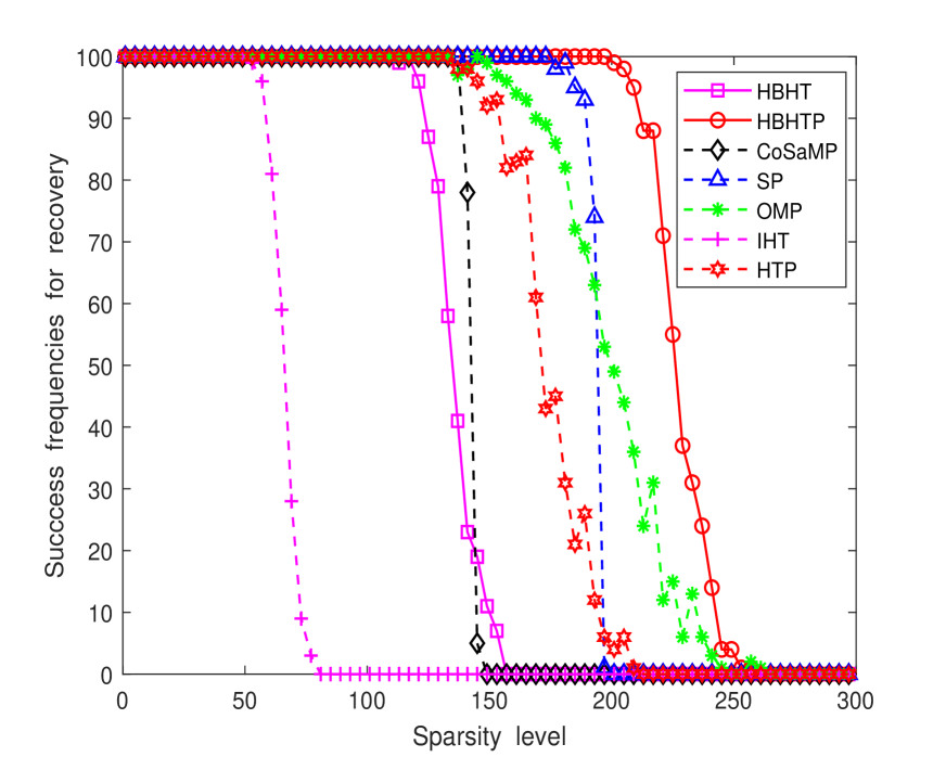
(a) Accurate measurements

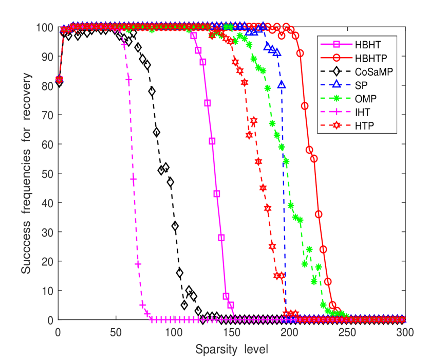
(b) Inaccurate measurements.

Figure 1: Comparison of success frequencies (rates) of algorithms for signal recovery with accurate and inaccurate measurements, respectively. The parameters $\alpha=1.5\times 10^{-3}$ and $\beta=0.6$ are set for HBHT and $\alpha=7\times 10^{-3}$ and $\beta=0.7$ for HBHTP.

5.1.1 Performance with unnormalized matrices

The performance of iterative-type thresholding methods is closely related to the choice of stepsize in each step. When $A$ is un-normalized/unscaled, initial simulations indicate that $\alpha=10^{-3}$ is a proper choice for IHT and HTP, $\alpha\in[10^{-3},2\times 10^{-3}]$ and $\beta\in(0,0.6]$ are proper choices for HBHT, and $\alpha\in[10^{-3},8\times 10^{-3}]$ and $\beta\in(0,0.7]$ are suitable for HBHTP, where the range for $\beta$ is implied from (27). We now start to compare algorithms using both accurate and inaccurate measurements. Given a random pair of $(A,x^{*}),$ the accurate and inaccurate measurements are given respectively by $y:=Ax^{*}$ and $y:=Ax^{*}+\epsilon h$, where $\epsilon=0.008$ and $h$ is a standard Gaussian random noise vector. We use the fixed parameters $\alpha=1.5\times 10^{-3}$ and $\beta=0.6$ in HBHT and $\alpha=7\times 10^{-3}$ and $\beta=0.7$ in HBHTP. The estimated success rates of the algorithms are shown in Fig. 1 in which the sparsity level $k$ is ranged from 1 to 297 with stepsize 4. It shows that the HBHTP generally outperforms the OMP, SP and HTP, and it might perform clearly better than CoSaMP, HBHT and IHT. We also observe from the experiments that the success rate of HBHT is slightly worse than that of CoSaMP in noiseless settings but it might be better than CoSaMP in noisy settings.

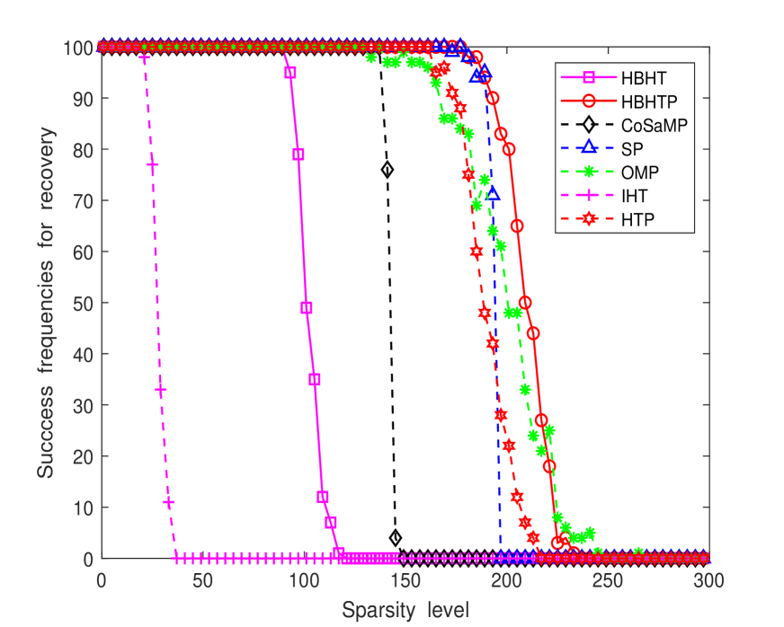
(a) Accurate measurements

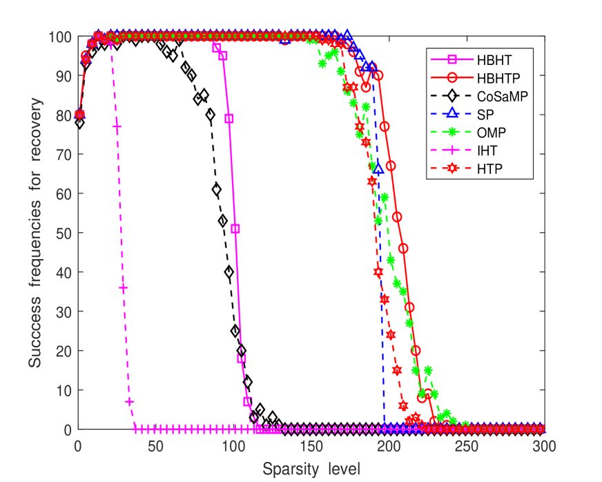
(b) Inaccurate measurements.

Figure 2: Comparison of success frequencies of algorithms with accurate and inaccurate measurements, respectively. The parameters $\alpha=0.6$ and $\beta=0.1$ are set in HBHT, and $\alpha=1.7$ and $\beta=0.7$ are set in HBHTP.

5.1.2 Performance with normalized matrices

The existing theory claims that the IHT and HTP with a larger stepsize such as $\alpha=1$ remains convergent if the matrix satisfies the RIP, and it is well known that the normalized Gaussian matrix $\bar{A}:=\frac{1}{\sqrt{m}}A$ may satisfy the RIP in high probability (see, e.g., Chapter 9 in [17] for details). In terms of a normalized matrix, the problem (1) is equivalent to $\underset{z}{\textrm{argmin}}\{{\left\lVert\bar{y}-\bar{A}z\right\rVert}_{2}^{2}:\left\lVert z\right\rVert_{0}\leq k\},$ where $\bar{y}=\frac{1}{\sqrt{m}}y$. The entries of such a normalized Gaussian matrix follow the distribution $\mathcal{N}(0,m^{-1})$. By taking into account the theoretical results in previous sections and testing for the values of parameters $(\alpha,\beta),$ we found the choices $\alpha\in[0.4+2\beta,1.6]$ and $\beta\in(0,0.6]$ are suitable for HBHT and $\alpha\in[0.3+2\beta,1.7]$ and $\beta\in(0,0.7]$ are suitable for HBHTP to achieve a good performance. We repeated the experiments in Section 5.1.1 by setting the stepsize $\alpha=1$ for IHT and HTP, the specific values $\alpha=0.6$ and $\beta=0.1$ for HBHT and $\alpha=1.7$ and $\beta=0.7$ for HBHTP. The results are demonstrated in Fig. 2 which appear to be similar to that of Fig. 1. However, one can observe that the normalization of the matrix, accordingly enlarged stepsize, and the choices of parameters do affect the recovery ability of HBHT, HBHTP, IHT and HTP to a certain degree. Again, it seems that the HBHTP performs generally better than other algorithms in noiseless and noisy settings, and the HBHT may perform better than CoSaMP and IHT in some noisy situations. Compared to IHT and HTP, the heavy-ball-based technique does play a vital role in speeding up and enhancing the performance of the traditional thresholding algorithms for sparse signal recovery.

5.1.3 Average number of iterations and time

We now compare the average number of iterations and CPU time required by several algorithms to meet the criterion (50) with accurate measurements. The testing environment is the same as Section 5.1.1. Within 50 iterations, if $x^{p}$ satisfies criterion (50), the algorithm terminates and the number of iterations $p$ is recorded. Otherwise, the number of iterations is recorded as 50. For OMP, the number of iterations is equal to the sparsity level of the input signal. Fig. 3(a) indicates that the average number of iterations required by HBHTP is lower than that of SP and HTP, and might be much lower than that of OMP, CoSaMP, HBHT and IHT especially when the sparsity level $k$ is high.

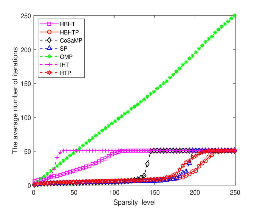
(a) Average number of iterations

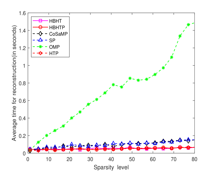
(b) Average CPU time

Figure 3: Comparison of average number of iterations and time taken by algorithms to meet the recovery criterion (50) with accurate measurements. The parameters $\alpha=0.6$ and $\beta=0.1$ are set in HBHT and $\alpha=1.7$ and $\beta=0.7$ in HBHTP.

Fig. 2(a) indicates that all $k$-sparse signals with $k\leq 80$ can be recovered by all mentioned algorithms except IHT. Thus we focus on the signals with sparsity levels $k\leq 80$ to compare the average time consumed by algorithms except IHT to meet the criterion (50). The results are demonstrated in Fig. 3(b), from which one can see that OMP takes more time than other algorithms to recovery the signal, and that the average time taken by SP, CoSaMP, HBHTP, HBHT and HTP increases slowly in a linear manner with respect to the sparsity level $k,$ and the average time consumed by SP and CoSaMP is approximately twice of HBHT, HBHTP and HTP. This indicates that the proposed algorithms have some advantage in time saving for signal recovery.

5.2 Phase transition

We further investigate and compare the performances of algorithms through the empirical phase transition curves (PTC) and algorithm selection maps (ASM) introduced in [1, 2]. All $m\times n$ matrices in this subsection are Gaussian random matrices with fixed $n=2^{12}$, whose entries are iid and follow the distribution $\mathcal{N}(0,m^{-1})$. The parameters $(\alpha,\beta)$ in HBHT and HBHTP are set exactly the same as in Section 5.1.2.

5.2.1 Phase transition curves

Denote by $\delta=m/n$ and $\rho=k/m.$ The phase transition curve of an algorithm separates the $(\delta,\rho)$ space into success and failure regions. The region below the curve, called recovery region, represents the problem instances with $(\delta,\rho)$ that can be exactly or approximately solved by the algorithm, while the region above the curve indicates the problem instances with $(\delta,\rho)$ to which the algorithm does not appear to find their correct solutions. The empirical phase transition curves demonstrated in this section are logistic regress curves identifying the 50% success rate for the given algorithm applying to a given problem class. This method was first introduced in [1, 2].

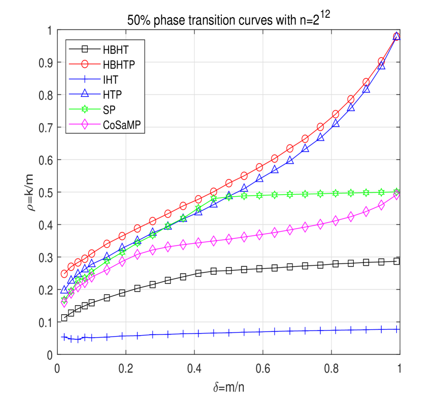
(a) Accurate measurements

(b) Inaccurate measurements

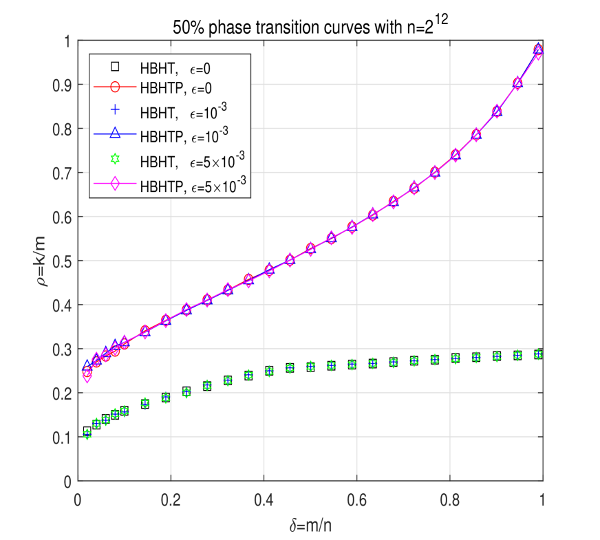
(c) Different noises

Figure 4: The $50\%$ success rate phase transition curves for six algorithms.

We now briefly introduce the mechanism for generating such a curve. The interested readers may find more detailed information about this from the references [1, 2]. To generate the PTC and ASM, we consider 25 different values of $m=\lceil\delta\cdot n\rceil$ where

$$\delta\in\{0.02,0.04,0.06,0.08\}\cup\{0.1,0.1445,\ldots,0.99\},$$ (51)

where the interval $[0.1,0.99]$ was equally divided into 20 parts. For every value of $m$, we collect 50 groups of sparsity levels $k=\lceil\rho\cdot m\rceil$ where $\rho$ is ranged from 0.02 to 1 with stepsize 0.02. For a fixed $m$, the recovery phase transition region for each algorithm is estimated by the interval $[k_{\min},k_{\max}]$, where $k_{\min}$ and $k_{\max}$ can be determined by a bisection method. They are the critical values to ensure that the recovery success rate is at least 90% for any $k<k_{\min}$ and at most 10% for any $k>k_{\max}$. For simplicity, we introduce the notations $k_{j}\stackrel{{\scriptstyle\Delta}}{{=}}k_{\min}+\lceil j\cdot\Delta k\rceil(j=0,1,\ldots,J)$, where $\Delta k=(k_{\max}-k_{\min})/J$ and $J=k_{\max}-k_{\min}$ if $k_{\max}-k_{\min}<50;$ otherwise $J=50.$ When estimating the success rate of an algorithm, $Nb=10$ problem instances are tested for each given $(k,m,n)$, where $k=k_{j},j=0,1,\ldots,J$. Based on the success rates, the phase transition curves can be obtained from the following logistic regression model [1, 2]:

$$\min_{(\gamma_{0},\gamma_{1})}\sum_{j=0}^{J}\left|g(k_{j}/m)-\frac{suc(k_{j},m,n)}{Nb}\right|,$$

where

$$g(\rho)=\frac{1}{1+exp[-\gamma_{0}(1-\gamma_{1}\rho)]},$$

and $suc(k_{j},m,n)$ is the number of recovery success among $Nb$ problem instances for each $(k_{j},m,n),j=0,1,\ldots,J.$ The 50% success recovery phase transition curves are defined by $g(\rho)=0.5.$

The curves for the algorithms HBHT, HBHTP, IHT, HTP, CoSaMP and SP are summarized in Fig. 4. In this comparison, the parameters $\alpha=0.6$ and $\beta=0.1$ are used in HBHT and $\alpha=1.7$ and $\beta=0.7$ in HBHTP. The accurate and inaccurate measurements are given by $y=Ax^{*}$ and $y=Ax^{*}+\epsilon h$, respectively, where $h$ is a standard Gaussian random vector and $\epsilon=0.001$. From Fig. 4 (a) and (b), we see that HBHTP has the highest phase transition curves. This indicates that HBHTP may outperform the other five algorithms for sparse signal recovery in both noiseless and noisy environments. One can also see that the phase transition curves of SP, CoSaMP, HBHT and IHT are below the line $\rho=0.5$ as $\delta\geq 0.5.$ This implies that the recovery performance of these algorithms would not remarkably be improved even when the number of measurements is increased. By contrast, the phase transition curves of HBHTP and HTP are twice as high as those of SP and CoSaMP as $\delta\rightarrow 1$. To see the influence of noise levels on the performance of algorithms, the phase transition curves for HBHT and HBHTP with three different noise levels $\epsilon\in\{0,10^{-3},5\times 10^{-3}\}$ are demonstrated in Fig. 4(c), from which one can observe that the curves of HBHT and HBHTP do not significantly change with respect to the noise level when the noise level is relatively low. This sheds light on the stability of the two algorithms in signal recovery.

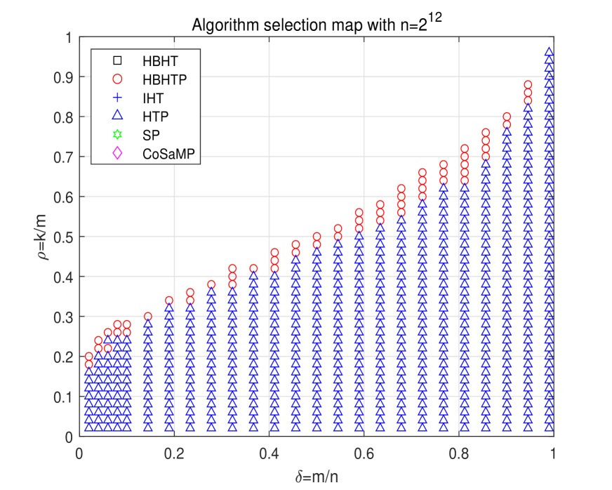
Figure 5: Selection map with accurate measurements.

5.2.2 Algorithm selection map

The intersection of the recovery regions below the phase transition curves indicates that multiple algorithms are capable of signal recovery. To choose an algorithm, one might also consider the computational time for recovery. As a result, the so-called algorithm selection map was introduced in [1, 2], which demonstrates the least average recovery time of the algorithms with accurate measurements. To draw an algorithm selection map, for each $\delta$ taking the values in (51), 10 problem instances are tested for every algorithm on the sampled phase space with the mesh $(\delta,\rho)$ with $\rho=\{j/50,j=1,2,\ldots,50\}$ until the success rate is lower than 90%. The algorithm with least computational time will be identified on the map. The map is shown in Fig. 5, which clearly depicts two regions in the phase plane, wherein HBHTP is the fastest algorithm for solving problem instances with relatively large $\rho,$ while the HTP reliably recovers the signal in least time in other cases.

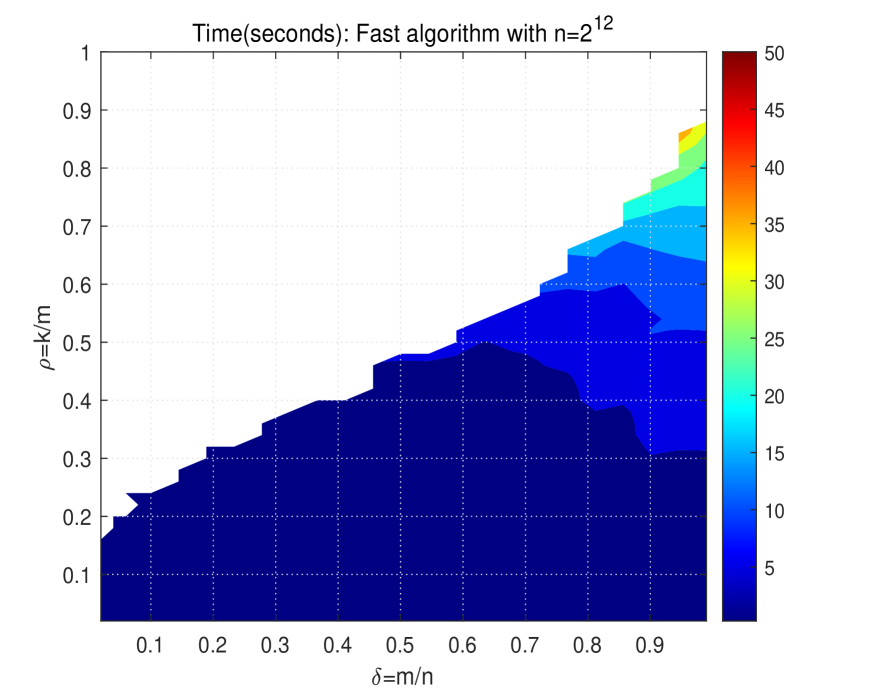
(a) Average time for the fastest algorithm

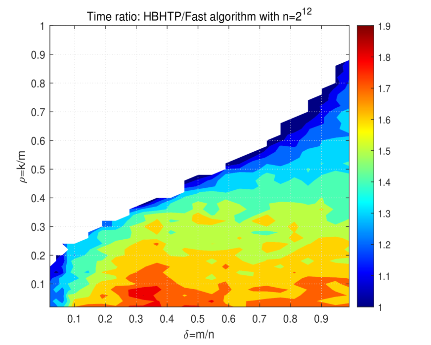
(b) HBHTP

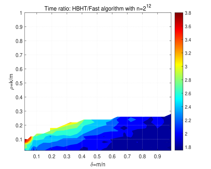
(c) HBHT

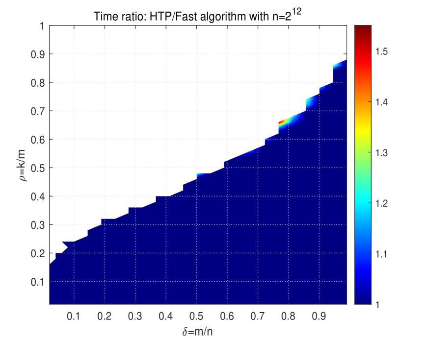
(d) HTP

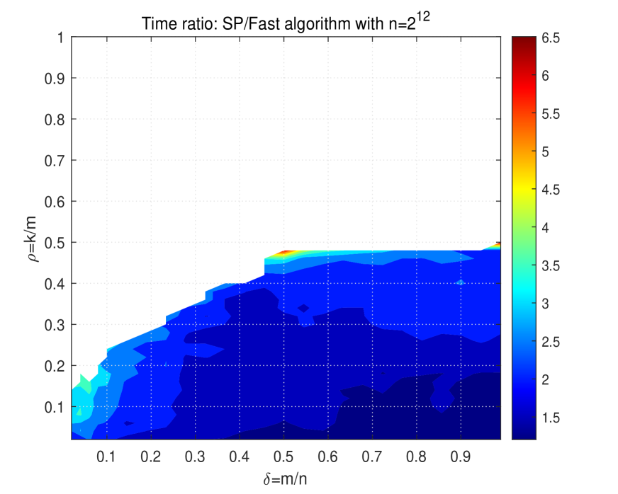
(e) SP

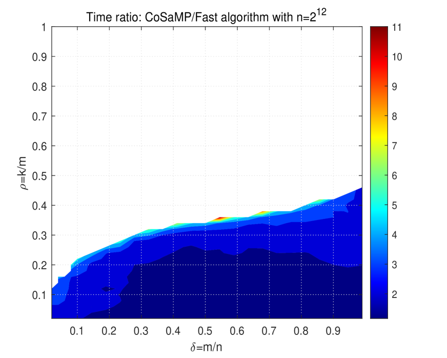
(f) CoSaMP

Figure 6: (a) The minimum average time of algorithms; (b)-(f) The ratios of average time for several algorithms against the fastest one.

After identifying the fastest algorithm, further information on the average recover time of algorithms are given in Fig. 6. The minimum average recovery time taken by an algorithm is displayed in Fig. 6(a). When $\rho\leq 0.3$, the minimal average run time of algorithms is close to each other for any $\delta\in(0,1)$. However, when $\rho>0.3$, we see that the larger the value of $\rho$, the more average run time is required by the algorithm when $\delta>0.6.$ The ratios of the average recovery time for the algorithms HBHTP, HBHT, HTP, SP and CoSaMP against that of the fastest algorithm are displayed in Fig. 6(b)-(f), respectively. Fig. 6(b) shows that the larger the value of $\rho$, the smaller the ratio for a fixed $\delta$, and the ratio for HBHTP is less than 1.5 when $\rho\geq 0.25$ or $\delta\leq 0.1.$ By contrast, Fig. 6(c)-(f) show that the larger the value of $\rho,$ the larger the ratios for those four algorithms. This phenomenon indicates that HBHTP might work better than other algorithms when the sparsity level $k$ is relatively high. We also observe that HBHTP and HTP are comparable to each other, and that HBHT, SP and CoSaMP often consume more than twice of the minimal average time. One can also observe that the ratios for SP and CoSaMP can be three and five times higher, respectively, when $\rho$ is large.

(a) $\delta=0.2780$

(b) $\delta=0.5005$

(c) $\delta=0.7230$

Figure 7: Average recovery time with respect to the change of $\rho$ under three different fixed values of $\delta.$

Finally, we demonstrate the change of average recovery time of algorithms against the factor $\rho.$ The results for three different parameters $\delta\in\{0.2780,0.5005,0.7230\}$ are given in Fig. 7. For $\rho\leq 0.2$, the average recover time of HBHTP, SP and CoSaMP are similar to each other. For $\rho\in[0.2,0.5]$, the time consumed by HBHTP and HTP increases slowly compared to that of SP and CoSaMP as the sparsity level $k$ increases. Moreover, the computational time of HTP approaches and surpasses that of HBHTP for $\rho\geq 0.4$ in Fig. 7(b) and for $\rho\geq 0.5$ in Fig. 7(c), respectively. Finally, we find that only HBHTP is typically able to recover the sparse signals fell into the region of the far right of Fig. 7(a)-(c). This provides some evidence to show that the HBHTP might admit a certain advantage in sparse signal recovery over several existing algorithms especially when $\rho$ is relatively large.

6 Conclusions

Incorporating the heavy-ball acceleration technique into the IHT and HTP methods leads to the HBHT and HBHTP algorithms for sparse signal recovery. The guaranteed performance of these algorithms has been established under the RIP assumption and certain conditions for the proper choice of the algorithmic parameters. The finite convergence and recovery stability of the algorithms were also shown in this paper. The numerical performance of the algorithms has been investigated from several difference perspectives including the recovery success rate, average number of iterations and computational times. Comparison of the proposed algorithms with a few existing ones is also made through the phase transition analysis including the phase transition cure and algorithm selection map. Simulations on random problem instances indicate that under proper choices of the algorithmic parameters, the algorithm HBHTP is an efficient algorithm for sparse signal recovery and it may outperform several existing algorithms in many cases.

References

- [1] J. D. Blanchard and J. Tanner. Performance comparisons of greedy algorithms in compressed sensing. Numer. Linear Algebra Appl., 22(2):254–282, 2015.
- [2] J. D. Blanchard, J. Tanner, and K. Wei. CGIHT: conjugate gradient iterative hard thresholding for compressed sensing and matrix completion. Information and Inference: A Journal of the IMA, 4(4):289–327, 2015.
- [3] T. Blumensath. Accelerated iterative hard thresholding. Signal Process., 92(3):752–756, 2012.
- [4] T. Blumensath and M. E. Davies. Iterative thresholding for sparse approximations. J. Fourier Anal. Appl., 14(5-6):629–654, 2008.
- [5] T. Blumensath and M. E. Davies. Iterative hard thresholding for compressed sensing. Appl. Comput. Harmon. Anal., 27(3):265–274, 2009.
- [6] T. Blumensath and M. E. Davies. Normalized iterative hard thresholding: Guaranteed stability and performance. IEEE J. Sel. Top. Signal Process., 4(2):298–309, 2010.
- [7] E. J. Candès and T. Tao. Decoding by linear programming. IEEE Trans. Inform. Theory, 51(12):4203–4215, 2005.
- [8] V. Cevher. On accelerated hard thresholding methods for sparse approximation. In Proceedings of SPIE Optical Engineering and Applications, Wavelets and Sparsity XIV, page 813811, 2011.
- [9] W. Dai and O. Milenkovic. Subspace pursuit for compressive sensing signal reconstruction. IEEE Trans. Inform. Theory, 55(5):2230–2249, 2009.
- [10] I. Daubechies, M. Defrise, and C. De Mol. An iterative thresholding algorithm for linear inverse problems with a sparsity constraint. Comm. Pure Appl. Math., 57(11):1413–1457, 2004.
- [11] G. M. Davis, S. G. Mallat, and Z. F. Zhang. Adaptive time-frequency decompositions. Opt. Eng., 33(7):2183–2191, 1994.
- [12] D. L. Donoho. De-noising by soft-thresholding. IEEE Trans. Inform. Theory, 41(3):613–627, 1995.
- [13] D. L. Donoho and J. M. Johnstone. Ideal spatial adaptation by wavelet shrinkage. Biometrika, 81(3):425–455, 1994.
- [14] M. Elad. Why simple shrinkage is still relevant for redundant representations? IEEE Trans. Inform. Theory, 52(12):5559–5569, 2006.
- [15] M. Elad. Sparse and redundant representations: From theory to applications in signal and image processing. Springer, NewYork, 2010.
- [16] S. Foucart. Hard thresholding pursuit: An algorithm for compressive sensing. SIAM J. Numer. Anal., 49(6):2543–2563, 2011.
- [17] S. Foucart and H. Rauhut. A mathematical introduction to compressive sensing. Springer, New York, 2013.
- [18] R. Garg and R. Khandekar. Gradient descent with sparsification: An iterative algorithm for sparse recovery with restricted isometry property. In Proceedings of the 26th International Conference on Machine Learning, Montreal, Canada, pages 337–344, 2009.
- [19] E. Ghadimi, H. R. Feyzmahdavian, and M. Johansson. Global convergence of the heavy-ball method for convex optimization. In 2015 European Control Conference, pages 310–315, 2015.
- [20] M. Gürbüzbalaban, A. Ozdaglar, and P. A. Parrilo. On the convergence rate of incremental aggregated gradient algorithms. SIAM J. Optim., 27(2):1035–1048, 2017.
- [21] K. Huang and S. Z. Zhang. A unifying framework of accelerated first-order approach to strongly monotone variational inequalities. arXiv:2103.15270v1, 2021.
- [22] R. Khanna and A. Kyrillidis. IHT dies hard: Provable accelerated iterative hard thresholding. In Proceedings of the Twenty-First International Conference on Artificial Intelligence and Statistics, 84:188–198, 2018.
- [23] A. Kyrillidis and V. Cevher. Matrix recipes for hard thresholding methods. J. Math. Imaging Vis., 48:235–265, 2014.
- [24] L. Lessard, B. Recht, and A. K. Packard. Analysis and design of optimization algorithms via integral quadratic constraints. SIAM J. Optim., 26(1):57–95, 2016.
- [25] J. Liu, A. Eryilmaz, N. B. Shroff, and E. S. Bentley. Heavy-ball: A new approach to tame delay and convergence in wireless network optimization. In IEEE INFOCOM 2016 - The 35th Annual IEEE International Conference on Computer Communications, pages 1–9, 2016.
- [26] N. Meng, Y. B. Zhao, M. Kočvara, and Z. F. Sun. Partial gradient optimal thresholding algorithms for a class of sparse optimization problems. J. Global Optim., https://doi.org/10.1007/s10898-022-01143-1, 2022.
- [27] D. Needell and J. A. Tropp. CoSaMP: Iterative signal recovery from incomplete and inaccurate samples. Appl. Comput. Harmon. Anal., 26(3):301–321, 2009.
- [28] P. Ochs, Y. J. Chen, T. Brox, and T. Pock. Ipiano: Inertial proximal algorithm for nonconvex optimization. SIAM J. Imaging Sci., 7(2):1388–1419, 2014.
- [29] B. T. Polyak. Some methods of speeding up the convergence of iteration methods. USSR Comput. Math. Math. Phys., 4(5):1–17, 1964.
- [30] B. T. Polyak. Introduction to optimization. Optimization Software, Inc. Publications Division, New York, 1987.
- [31] J. Shen and P. Li. A tight bound of hard thresholding. J. Machine Learning Res., 18(208):1–42, 2018.
- [32] T. Sun, D. S. Li, Z. Quan, H. Jiang, S. G. Li, and Y. Dou. Heavy-ball algorithms always escape saddle points. arXiv:1907.09697v1, 2019.
- [33] W. Tao, S. Long, G. W. Wu, and Q. Tao. The role of momentum parameters in the optimal convergence of adaptive Polyak’s heavy-ball methods. arXiv:2102.07314v1, 2021.
- [34] J. A. Tropp and A. C. Gilbert. Signal recovery from random measurements via orthogonal matching pursuit. IEEE Trans. Inform. Theory, 53(12):4655–4666, 2007.
- [35] H. B. Wang and P. C. Miller. Scaled heavy-ball acceleration of the Richardson-Lucy algorithm for 3D microscopy image restoration. IEEE Trans. Image Process., 23(2):848–854, 2014.
- [36] R. Xin and U. A. Khan. Distributed heavy-ball: A generalization and acceleration of first-order methods with gradient tracking. IEEE Trans. Autom. Control, 65(6):2627–2633, 2020.
- [37] Y. B. Zhao. Sparse optimization theory and methods. CRC Press, Boca Raton, FL, 2018.
- [38] Y. B. Zhao. Optimal -thresholding algorithms for sparse optimization problems. SIAM J. Optim., 30(1):31–55, 2020.
- [39] Y. B. Zhao and Z. Q. Luo. Improved RIP-based bounds for guaranteed performance of two compressed sensing algorithms. arXiv:2007.01451v3, 2020.
- [40] Y. B. Zhao and Z. Q. Luo. Analysis of optimal thresholding algorithms for compressed sensing. Signal Process., 187:108148, 2021.