Genuinely Multipartite Entanglement vias Shallow Quantum Circuits

Abstract

Multipartite entanglement is of important resources for quantum communication and quantum computation. Our goal in this paper is to characterize general multipartite entangled states according to shallow quantum circuits. We firstly prove any genuinely multipartite entanglement on finite-dimensional spaces can be generated by using 2-layer shallow quantum circuit consisting of two biseparable quantum channels, which the smallest nontrivial circuit depth in the shallow quantum circuit model. We further propose a semi-device-independent entanglement model depending on the local connection ability in the second layer of quantum circuits. This implies a complete hierarchy of distinguishing genuinely multipartite entangled states. It shows a completely different multipartite nonlocality from the quantum network entanglement. These results show new insights for the multipartite entanglement, quantum network, and measurement-based quantum computation.

Introduction

Entanglement is an important quantum property of two or more systems in quantum mechanics associated with Schrödinger evolution equations Schr . A bipartite entanglement is defined as its cannot be decomposed into an ensemble of separable states. This allows verifying any bipartite entanglement beyond all separable states using entanglement witness HHH . Another device-independent method is inspired by Einstein-Podolsky-Rosen (EPR) steering EPR or Bell inequality Bell ; CHSH ; Brun ; Luo1 ; TPL which can witness stronger quantum nonlocalities from only the statistics of local measurements on an entanglement Wise .

Although the fully separable model is easily extended for multi-particle systems, it is useless for verifying the genuinely multipartite nonlocality. Instead, some stronger separable models are constructed for special goals. One is the so-called biseparable model Sv which is defined to distinguish the genuinely multipartite entanglement from all the biseparable states. This allows us to witness the genuine multipartite nonlocality beyond the fully separable model even for quantum networks Luo22 . Another model is using GHZ-paradox GHZ ; tang ; Liu ; Luois in the all-versus-nothing test manner. If the local tensor decomposition is considered, the high-dimensional model Kraft18 ; Des ; EKZ or quantum network entanglement may rule out any network separable state consisting of small entanglements that are shared by partial parties NWR ; Kraft ; Luo2021 . Different from the biseparable model Sv , this model provides a device-independent verification of unknown entanglement devices. Another is from the particle-losing model for characterizing the entanglement robustness against losing partial systems QABZ ; BPB ; Luo2022 . This can imply a different hierarchy of well-known entanglements including GHZ state and Dicke states going beyond other models Sv ; NWR ; Kraft ; Luo2021 . All of these entanglement models can only justify special multipartite systems. A natural problem is to explore proper model for general systems.

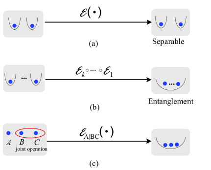
Figure 1: Schematic shallow quantum circuit for quantum state generations. (a) A bipartite separable system with a 1-layer quantum circuit. $\mathcal{E}(\cdot)$ is a bipartite separable channel defined by $\mathcal{E}(\cdot)=\sum_{i}K_{i}\otimes S_{i}\left(\cdot\right)K_{i}^{\dagger}\otimes S_{i}^{\dagger}$, where Kraus operators $K_{i}$ and $S_{i}$ satisfy $\sum_{i}K_{i}^{\dagger}{}K_{i}\otimes S_{i}^{\dagger}S_{i}=\openone$ with the identity operator $\openone$. (b) An $n$-partite entanglement with $k$-layer quantum circuits. Each $\mathcal{E}_{j}(\cdot)$ is a biseparable quantum channel. (c) A tripartite entanglement with 2-layer quantum circuits. One is from a biseparable quantum channel and the other is from a local joint model in adversarial scenarios. Here, two parties in the second layer who share particles $B$ and $C$ may perform local joint operations defined by a biseparable quantum channel $\mathcal{E}_{A|BC}(\cdot)$ over the bipartition $A$ and $\{B,C\}$.

Bravyi et al. Bra investigated 2D Hidden Linear Function problem in terms of constant-depth quantum circuit using special quantum gates. This is further extended to other circuits over special gates Watt . These results intrigue new ideas to explore multipartite entanglement with shallow quantum circuits. Especially, each bipartite separable state can be generated by using one layer of quantum separable channel, as Fig.1(a). This suggests a novel model for generating multipartite entanglement by using different layers of biseparable completely-positive trace-preserving (BCPTP) channels Sv from fully separable states, as shown in Fig.1(b). A nature problem is what’s the relationship among the entangled states, circuit depth and quantum channels.

The goal of this work is to characterize multipartite entanglement based on shallow quantum circuits of bipartite quantum channels. We firstly prove any multipartite entanglement can be generated by using a 2-layer shallow quantum circuit consisting of two biseparable completely-positive trace-preserving channels. If the second layer consists of a convex combination of local fully separable channels with one joint channel, the present model further implies a complete hierarchy for characterizing any multipartite entanglement according to the joint ability in its generation circuits. This second layer can be further regarded as an adversarial model in cryptographic applications such as quantum secret sharing HB , as shown in Fig.1(c). The present model provides a simple method to characterize general multipartite entanglement using Schmidt numbers of reduced density matrices. Its shows a different multipartite nonlocality from previous models Luo2022 ; NWR ; Kraft ; Luo2021 .

Result

Genuinely multipartite entanglement generated with shallow quantum circuits

A general isolated $d$-dimensional quantum system is represented by a normalized vector $|\phi\rangle$ in Hilbert space $\mathcal{H}_{d}$. Instead, an open system is described by probabilistically mixing an ensemble of pure states $\{|\phi_{i}\rangle\}$, that is, $\rho=\sum_{i}p_{i}|\phi_{i}\rangle\langle\phi_{i}|$, where $\{p_{i}\}$ is a probability distribution. An $n$-particle pure state $|\Phi\rangle$ on Hilbert space $\otimes_{i=1}^{n}\mathcal{H}_{A_{i}}$ is biseparable Sv if it can be represented by $|\Phi\rangle=|\phi\rangle_{I}|\psi\rangle_{\overline{I}}$ with two pure states $|\phi\rangle$ and $|\psi\rangle$, where $I$ and $\overline{I}$ are bipartition of $\{A_{1},\cdots,A_{n}\}$. Note that $|\Phi\rangle$ can be generated from a fully separable state $|0\rangle^{\otimes n}$ with a 1-layer shallow circuit of biseparable quantum channel defined by $\mathcal{E}(\cdot):=U_{I}\otimes V_{\overline{I}}(\cdot)U_{I}^{\dagger}\otimes V_{\overline{I}}^{\dagger}$, that is,

$$|\Phi\rangle=(U_{I}\otimes V_{\overline{I}})|0\rangle^{\otimes n}$$ (1)

where $U_{I}(\otimes_{A_{i}\in I}|0\rangle_{A_{i}})=|\phi\rangle_{I}$ and $V_{\overline{I}}(\otimes_{A_{j}\in\overline{I}}|0\rangle_{A_{j}})=|\psi\rangle_{\overline{I}}$. This intrigues a multipartite entanglement model in terms of shallow quantum circuits. Especially, define a biseparable completely positive trace-preserving (BCPTP) channel Werner ; Sv on Hilbert space $\mathcal{H}_{I}\otimes\mathcal{H}_{\overline{I}}$ as

$$\mathcal{E}_{I}(\rho)=\sum_{i}(K_{i}\otimes S_{i})\rho(K_{i}^{\dagger}\otimes S_{i}^{\dagger})$$ (2)

where $K_{i},S_{i}$ are respective Kraus operators on Hilbert space $\mathcal{H}_{I}$ and $\mathcal{H}_{\overline{I}}$ and satisfy $\sum_{i}K_{i}^{\dagger}K_{i}\otimes S_{i}^{\dagger}S_{i}=\openone$ with the identity operator $\openone$, $\mathcal{H}_{I}=\otimes_{A_{i}\in I}\mathcal{H}_{A_{i}}$, and $\mathcal{H}_{\overline{I}}=\otimes_{A_{j}\in\overline{I}}\mathcal{H}_{A_{j}}$. For a given biseparable state $\rho_{bs}=\sum_{i}p_{i}\rho_{i|I}\otimes\varrho_{i|\overline{I}}$ over a given bipartition $I$ and $\overline{I}$, it is straightforward to show from Eq.(2) that there is a BCPTP channel $\mathcal{E}_{I}$ with $K_{i}:|0\rangle\mapsto\rho_{i|I}$ and $S_{i}:|0\rangle\mapsto\varrho_{i|\overline{I}}$ such that

$$\rho_{bs}=\mathcal{E}_{I}(|0\rangle\langle 0|^{\otimes n})$$ (3)

This means that any biseparable state Sv can be generated by a probabilistically convex combination of BCPTP channels, that is,

$$\rho_{bs}=\mathcal{E}(|0\rangle\langle 0|^{\otimes n})=\sum_{I}q_{I}\mathcal{E}_{I}(|0\rangle\langle 0|^{\otimes n})$$ (4)

where the summation is over any proper subset of $\{A_{1},\cdots,A_{n}\}$. Thus BCPTP channel provides an equivalent representation of the biseparable model Sv . Our goal in what follows is to explore the multipartite entanglement in terms of its shallow generation circuits consisting of BCPTP channels.

Note that one layer of BCPTP channel can only build a biseparable state Sv . This implies that the nontrivial example should be at least two layers. Especially, for any genuinely $n$-partite entanglement on finite-dimensional Hilbert spaces $\otimes_{i=1}^{n}\mathcal{H}_{A_{i}}$ Sv , assume that the Schmidt decomposition with respect to the bipartition $I=\{A_{1}\}$ and $\overline{I}=\{A_{2},\cdots,A_{n}\}$ is given by

$$|\Phi\rangle=\sum_{i=1}^{d}\sqrt{\lambda_{i}}|\phi_{i}\rangle_{I}|\psi_{i}\rangle_{\overline{I}},$$ (5)

where $\lambda_{i}$’s are Schmidt coefficients satisfying $\sum_{i=1}^{d}\lambda_{i}=1$, $\{|\phi_{i}\rangle\}$ are orthogonal states of $A_{1}$, and $\{|\psi_{i}\rangle\}$ are orthogonal states of all the systems in $\overline{I}$. There is a unitary transformation $U$ on Hilbert space $\mathcal{H}_{\overline{I}}$ satisfying (Supplementary note 1):

$$U:|\psi_{i}\rangle_{\overline{I}}\mapsto|0\rangle_{A_{2}}|\hat{\psi}_{i}\rangle_{J},i=1,\cdots,d$$ (6)

where $\{|\hat{\psi}_{i}\rangle\}$ are orthogonal states of all the systems in $J:=\{A_{3},\cdots,A_{n}\}$. Thus the state $|\Phi\rangle$ is generated by a 2-layer shallow quantum circuit consisting of two BCPTP channels. By considering the probabilistic mixture of BCPTP channels, it implies a general result for multipartite entanglement on finite-dimensional Hilbert spaces.

Theorem 1. For $n$-partite state $\rho$ on finite-dimensional Hilbert spaces, it can be generated by a 2-layer quantum circuit given by

$$\rho = \mathcal{E}_{2}\circ\mathcal{E}_{1}(|0\rangle\langle 0|^{\otimes n})$$ (7)

$$= \sum_{I,J}p_{I}q_{J}\mathcal{E}_{J}\circ\mathcal{E}_{I}(|0\rangle\langle 0|^{\otimes n})$$ (8)

where $\mathcal{E}_{1}$ and $\mathcal{E}_{2}$ are respective probabilistic mixtures of BCPTP channels $\mathcal{E}_{I}$ and $\mathcal{E}_{J}$, and $\{p_{I}\}$ and $\{q_{J}\}$ are probability distributions.

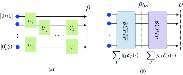
Figure 2: Schematic quantum circuit for generating a general state. (a) Standard quantum circuit model with different depths. Here, $U_{i}$ are two-particle universal logical gates Deut ; Vlas . (b) The present circuit model with two-depth. There are two BCPTP channels $\sum_{I}p_{I}\mathcal{E}_{I}(\cdot)$ and $\sum_{J}q_{J}\mathcal{E}_{J}(\cdot)$ over different bipartitions $I,\overline{I}$ and $J,\overline{J}$.

Theorem 1 holds for any pure or mixed state on finite-dimensional Hilbert space. Eq.(8) implies a universal circuit with two depths for building any state from a fully product state, as shown in Fig.2. This means any entanglement can be generated by a 2-layer shallow circuit consisting of two BCPTP channels. Note that the 2-layer quantum circuit is the smallest nontrivial shallow circuits. Theorem 1 implies the strong generation ability of small shallow circuits. This arises an immediate problem whether or not similar result holds in infinite-dimensional Hilbert spaces.

The present shallow circuit consisting of BCPTP channels is stronger than the standard quantum circuit model with an unfixed circuit depth using two-particle joint operations Deut ; Vlas . The second layer circuit of Theorem 1 means that the BCPTP channel may activate multipartite entanglement from biseparable states. This kind of entanglement swapping is the core of quantum networks BBC ; Kimble .

$k$-connection genuinely entanglement generated with 2-layer shallow quantum circuits

In Theorem 1, a two-layer circuit model may be too strong both in theory and applications. The main reason is that both biseparable quantum channels allow any bipartition decomposition. Instead, we consider a one-side biseparable channel in the second layer while the first layer is to prepare a biseparable state. Here, one local joint operation $\mathcal{E}_{I}$ may be performed on a local set $I\subset\{A_{1},\cdots,A_{n}\}$ while separable operations are performed on each particle in the complement set $\overline{I}$. The joint channel $\mathcal{E}_{I}$ can be regarded as semi-device-independent scenarios in secure applications such as quantum secret sharing, as shown in Fig.1(c), where partial adversaries who own systems in $I$ may cooperate to recover other parties’ information by performing joint operations while legal others are remote distributed and then not allowed to perform joint operations. Denote $\ell_{I}$ as the number of particles in $I$. Define a $k$-connection BCPTP channel $\mathcal{E}_{I}^{(k)}$ on Hilbert space $\mathcal{H}_{I}\otimes\mathcal{H}_{\overline{I}}$ with $\ell_{I}\leq k$ as

$$\mathcal{E}_{I}^{(k)}(\rho)=\sum_{i}(K_{i}\otimes(\otimes_{j\in\overline{I}}S_{i;j}))\rho(K_{i}^{\dagger}\otimes(\otimes_{j\in\overline{I}}S_{i;j}^{\dagger}))$$ (9)

where $K_{i}$ and $S_{i;j}$ are respective Kraus operators on Hilbert space $\mathcal{H}_{I}$ and $\mathcal{H}_{A_{j}}$, and satisfy $\sum_{i}(K_{i}^{\dagger}K_{i}\otimes(\otimes_{j\in\overline{I}}S_{i;j}^{\dagger}S_{i;j}))=\openone$. The present $k$-connection BCPTP channel is of state-dependent. Our goal here is to explore genuinely multipartite entanglement in terms of its generation circuits with the quantum channel (9) in the second layer.

Definition 1. An $n$-partite state is $k$-connection genuinely entanglement ($k$-CGE) if it is not a $k$-connection biseparable state given by

$$\rho_{bs}^{(k)}=\sum_{\ell_{I}\leq k}p_{I}\mathcal{E}_{I}^{(\ell_{I})}\circ\mathcal{E}_{1}(|0\rangle\langle 0|^{\otimes n})$$ (10)

where $\mathcal{E}_{I}^{(\ell_{I})}$ are $\ell_{I}$-connection BCPTP channels in terms of the bipartition $I$ and $\overline{I}$, $\{p_{I}\}$ is a probability distribution, and $\mathcal{E}_{1}$ is a convex combination of BCPTP channels.

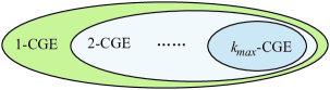
Figure 3: Schematic hierarchy of genuinely $n$-partite entanglement. The set consisting of $k$-CGE is included in the set consisting of $k-1$-CGE. The largest set consists of 1-CGE while the smallest set contains $k_{\max}$-CGE with $k_{\max}=\lfloor\frac{n}{2}\rfloor$, where $\lfloor x\rfloor$ denotes the maximal integer no more than $x$.

Similar to the proof of Theorem 1, the Schmidt decomposition of a given $n$-particle pure state $|\Phi\rangle$ on $d^{n}$-dimensional Hilbert space $\otimes_{i=1}^{n}\mathcal{H}_{A_{i}}$ is given by

$$|\Phi\rangle=\sum_{i=1}^{N}\sqrt{\lambda_{i}}|\phi_{i}\rangle_{I}|\psi_{i}\rangle_{\overline{I}}$$ (11)

where $\lambda_{i}$’s are Schmidt coefficients satisfying $\sum_{i=1}^{N}\lambda_{i}=1$, $\{|\phi_{i}\rangle\}$ are orthogonal states of all the systems in $I$, $\{|\psi_{i}\rangle\}$ are orthogonal states of all the systems in $\overline{I}$. From Eq.(11) we have $N\leq\min\{d^{\ell_{I}},d^{n-\ell_{I}}\}$. This implies that $N\leq d^{n-\ell_{I}}\leq d^{n/2-1}$ for any integer $\ell_{I}$ with $\ell_{I}\geq n/2+1$. There is a unitary transformation $U$ on Hilbert space $\mathcal{H}_{I}$ satisfying

$$U:|\psi_{i}\rangle_{I}\mapsto|0\rangle_{A_{j}}|\hat{\psi}_{i}\rangle_{J},i=1,\cdots,N$$ (12)

where $A_{j}\in\overline{I}$ and $\{|\hat{\psi}_{i}\rangle\}$ are orthogonal states of the particles in $J:=\overline{I}-\{A_{j}\}$. So, the state $|\Phi\rangle$ is an $\ell_{I}$-connection biseparable. This implies a general result for generating multipartite entanglement with different connection abilities as follows.

Theorem 2. For an $n$-partite state $\rho$ on finite-dimensional Hilbert space, it can be generated by a $2$-layer shallow quantum circuit as

$$\rho = \mathcal{E}_{2}^{(k)}\circ\mathcal{E}_{1}(|0\rangle\langle 0|^{\otimes n})$$ (13)

$$= \sum_{I,J}p_{I}q_{J}\mathcal{E}_{J}^{(k)}\circ\mathcal{E}_{I}(|0\rangle\langle 0|^{\otimes n})$$ (14)

where $\mathcal{E}_{1}$ is a convex combination of BCPTP channels $\mathcal{E}_{I}$ and $\mathcal{E}_{2}^{(k)}$ is a convex combination of $k$-connection BCPTP channels $\mathcal{E}_{J}^{(k)}$ defined in Eq.(9) with $k\geq n/2+1$.

Theorem 2 rules out the possibility of $k$-CGE for large integer $k$. The situation is different for small $k$. For special case of $n=2$, Definition 1 is reduced to the standard separable model of bipartite systems Schr ; HHH . For each $n\geq 3$, from Definition 1 any biseparable state Sv is $1$-connection biseparable state. In general, the connection ability $k$ is state-dependent.

A complete hierarchy of genuinely multipartite entanglement

Note that any $k$-connection biseparable state is an $s$-connection biseparable state for any $s\geq k$. This implies a complete hierarchy for all the multipartite entangled states, as shown in Fig.3. The largest set contains $1$-CGEs, that is, the genuinely multipartite entanglement in the biseparable model Sv . Instead, the smallest set consists of the strongest multipartite entanglement, that is, $k_{\max}$-CGE with $k_{\max}=\lfloor\frac{n}{2}\rfloor$. Since each subset of $k$-CGE is not empty (see examples in what follows), the new classification is strict from Theorems 1 and 2, that is, each entanglement belongs to the only set $k$-CGE while it is not in $k+1$-CGE for some $k$.

For any $n$-particle pure state $|\Phi\rangle$ on a finite-dimensional Hilbert space $\otimes_{i=1}^{n}\mathcal{H}_{A_{i}}$, from Eq.(11) the orthogality of $\{|\phi_{i}\rangle_{I}\}$ allows for constructing a unitary transformation (12) if and only if its Schmidt number satisfies $N\leq d^{k-1}$ with $\ell_{I}=k$. This implies a directive way to find the connection-ability $k$ for a given pure state using its Schmidt numbers of reduced density matrices (Supplementary note 2).

Theorem 3. An $n$-partite pure state on a $d^{n}$-dimensional Hilbert space $\otimes_{i=1}^{n}\mathcal{H}_{A_{i}}$ is $k$-CGE if and only if the Schmidt number of the reduced density matrix of any $k$ particles is larger than $d^{k-1}$.

From Definition 1 any genuinely multipartite entanglement in the biseparable model Sv ; See is 1-CGE. Moreover, the present $k$-CGE is stronger than the robust entanglement with the robustness-depth $k$ since the particle-losing channel Luo2022 is local CPTP channel. From Theorem 3 it generally requires to evaluate Schmidt numbers of almost all the reduced density matrices of $s$-particle with $s\leq 2^{n}$. This yields to a NP hard problem for general entanglement because of exponential number ($O(d^{2/n})$) of reduced states. Instead, it is easy for special states.

Examples

Example 1. An $n$-partite Greenberger-Horne-Zeilinger (GHZ) state GHZ is given by

$$|GHZ\rangle=\sum_{i=1}^{d}a_{i}|i\cdots{}i\rangle_{A_{1}\cdots{}A_{n}}$$ (15)

where $a_{i}$’s satisfy $\sum_{i=1}^{d}a_{i}^{2}=1$. It is easy to verify the state (15) is 1-CGE from its permutational symmetry.

Example 2. Consider an $n$-partite W-type state Dur :

$$|W\rangle_{A_{1}\cdots{}A_{n}}=\sum_{i=1}^{d}a_{i}|1_{i}\rangle+a_{n+1}|1\cdots 1\rangle$$ (16)

where $|1_{i}\rangle$ denotes the $i$-excitation defined by $|1_{i}\rangle=|0\rangle^{\otimes i-1}|1\rangle|0\rangle^{\otimes n-i}$. From Theorem 3 it is easy to prove $|W\rangle$ is a 2-CGE for $a_{i}\not=0$, $i=1,\cdots,n+1$. This can be extended for general $n$-qudit Dicke states with $s$ excitations Dicke given by

$$|D_{s,n}\rangle=\frac{1}{\sqrt{L_{s}}}\sum_{i_{1}+\cdots{}+i_{n}=s}|i_{1}\cdots{}i_{n}\rangle_{A_{1}\cdots{}A_{n}}$$ (17)

where $L_{s}$ is the normalization constant. It is a $k$-CGE with $k=\lfloor\log_{d}(s+1)\rfloor+1$ (Supplementary note 3). This is beyond previous models Sv ; See which do not distinguish GHZ state and W state. Moreover, the state $|D_{s,n}\rangle$ is equivalent to $|D_{(d-1)^{n}-s,n}\rangle$ under local unitary operations. This implies the strongest nonlocality of Dicke state $|D_{s,n}\rangle$ with $s=\lfloor(d-1)^{n}/2\rfloor$.

Example 3. Another example is entangled quantum network which may show different nonlocalities beyond single entanglement RBBB ; Brun ; Luo1 . As resource states of measurement-based quantum computation cluster , the so-called cluster states cluster may be generated by generalized Einstein-Podolsky-Rosen (EPR) states EPR , as shown in Fig.4. This kind of entanglement is 1-CGE (Supplementary note 4). Similar result can be extended for generalized graph states graph consisting of generalized EPR EPR and GHZ states GHZ . Instead, some quantum networks may show different connection abilities. One example is the $n$-partite completely-connected network $\mathcal{N}_{c}$, where each pair shares one bipartite entanglement $|\phi_{ij}\rangle$. Recent result shows the joint state of any $k$-partite subnetwork in $\mathcal{N}_{c}$ is entangled for $k\geq 2$ Luo2022 ; Sv . Hence, from Theorems 2 and 3 the joint state of $\mathcal{N}_{c}$ is a $k_{\max}$-CGE with $k_{\max}=\lfloor\frac{n}{2}\rfloor$. This means that $\mathcal{N}_{c}$ shows stronger nonlocality than GHZ state (15) and W state (16) for any $n>4$ in the present model. This is different from the robust-entanglement model Luo2022 , where both the W state and $\mathcal{N}_{c}$ has the same robust-depth. Remarkably, it is converse to the recent result NWR ; Kraft ; Luo2021 which proves GHZ and W states have stronger entanglement beyond quantum networks. This shows a surprising feature of the genuinely multipartite nonlocality beyond bipartite scenarios, that is, it is of model-dependent.

For general quantum networks, it is general difficult to find the largest $k$ such that the total state of $\mathcal{N}_{q}$ is $k$-CGE. Here, we provide a polynomial-time algorithm (Algorithm 1) for estimating the upper bound of $k$ for featuring its connection ability. This is inspired by Lemmas 1 and 2 (Supplementary note 5).

Input: Finite-size network $\mathcal{N}_{q}$

Output: $k$, satisfying that $\mathcal{N}_{q}$ is at most $k$-connection entanglement

• Find the connectedness degree $\ell_{i}$ for any each party $\textsf{A}_{i}$ with $i=1,\cdots,n$.

• Rearrange all parties with decreasing order into $\textsf{A}_{1},\cdots,\textsf{A}_{n}$ (for simplicity).

• Find $J$ such that $\ell_{j}=\min\{\ell_{i}\}$ with $j\in J$. Let $m=|J|$.

• For $s=1:m$

• For $t=1:\lfloor\frac{\ell_{j}+1}{2}\rfloor$

• (a) Let $\mathcal{A}_{1}=\{\textsf{A}_{j}\}$ and $\overline{\mathcal{A}}_{t}=\{\textsf{A}_{1},\cdots,\textsf{A}_{n}\}-\mathcal{A}_{t}$.

• (b) Let $\mathcal{A}_{t+1}=\mathcal{A}_{t}\cup\{\textsf{A}_{u}\}$, where $\textsf{A}_{u}$ has shared the most bipartite entangled states with parties in $\mathcal{A}_{t}$ compared with other parties in $\overline{\mathcal{A}}_{t}$, and $\textsf{A}_{u}\in\overline{\mathcal{A}}_{t}$.

• (c) Evaluate $s_{j;in}$ and $t_{j}$.

• (d) If $s_{j;in}+2t_{j}<s_{j;out}$

• $t\to t+1$

• Otherwise

• Return $v_{s}=\min\{\ell_{j},t\}$

• $s\to s+1$

• Output $k\leq\min\{v_{1},\cdots,v_{m}\}$

Algorithm 1 Verifying any $n$-partite quantum network $\mathcal{N}_{q}$ consisting of bipartite entanglement

For each party $\textsf{A}_{j}$ with the minimal connectedness degree $\ell_{j}$, from Lemma 1 (Supplementary note 5) if $s_{j;in}+2t_{j}\geq s_{j;out}$ for some $t$ there is a CPTP mapping to disentangle all the particles shared by $\textsf{A}_{j}$. Hence, the total state of $\mathcal{N}_{q}$ is $t$-connection biseparable. The time complexity of the step (i) is at most $O(n^{2})$. The time complexity of the step (iii) is at most $O(n)$. For a given party $\textsf{A}_{j}$ with $j\in J$, the time complexity of the step (b) is at most $O(n^{2})$. Hence, the total time complexity is at most $O(n^{4})$.

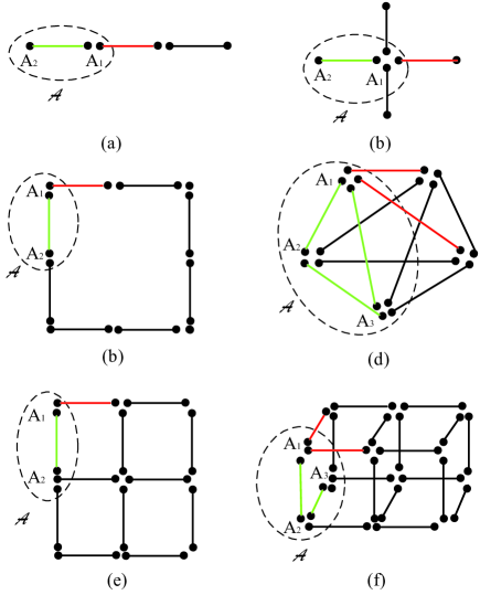
Figure 4: Schematic quantum networks. (a) Chain quantum network. (b) Star quantum network. (c) Cyclic quantum network. (d) Completely connected quantum network. (e) Planar quantum network (or cluster states). (d) Cubic quantum network (or cluster states). Here, each line with two dots denotes one bipartite entanglement. $\mathcal{A}$ denotes the set consisting of all parties who cooperate to disentangle the party $\textsf{A}_{1}$. The red lines denote the bipartite entangled states shared by $\textsf{A}_{1}$ with others out of $\mathcal{A}$. The green lines denote the bipartite entangled states shared by the parties in $\mathcal{A}$.

Some examples are shown in Fig.4. For the chain quantum network in Fig.4(a), the party $\textsf{A}_{1}$ shares one bipartite entanglement (red line) with other parties out of $\mathcal{A}$, and shares one bipartite entanglement (green line) with $\textsf{A}_{2}$. From Lemma 1 the chain quantum network in Fig.4(a) is 2-connection biseparable, where the party $\textsf{A}_{1}$ can be disentangled with other parties out of $\mathcal{A}$ by using joint operation of $\textsf{A}_{1}$ and $\textsf{A}_{2}$. Moreover, it is genuinely multipartite entanglement Luo2021 ; Sv , that is, any local operation cannot disentangle one party. Thus the chain quantum network in Fig.4(a) is 1-CGE. Similar result holds for the star quantum network in Fig.4(b) and cyclic quantum network in Fig.4(c). For a completely connected quantum network in Fig.4(d), the party $\textsf{A}_{1}$ shares two bipartite entangled states (red lines) with others out of $\mathcal{A}$. There are three bipartite entangled states (green lines) shared by parties in $\mathcal{A}$. From Lemma 1, it is 3-connection biseparable while any two parties cannot jointly disentangle one party. Hence, this quantum network is 2-CGE, where the party $\textsf{A}_{1}$ can be disentangled with others out of $\mathcal{A}$ by using joint operation of the parties $\textsf{A}_{1},\textsf{A}_{2}$ and $\textsf{A}_{3}$. In general, we can prove an $n$-partite completely connected network is $k_{\max}$-CGE with $k_{\max}=\lfloor\frac{n}{2}\rfloor$. Similarly, from Lemma 2 the planar quantum network in Fig.4(e) is 1-CGE while the cubic quantum network is 2-CGE.

Robustness of $k$-CGE

From Eq.(10) all the $k$-connection biseparable states constitutes a convex set $\mathcal{S}_{k}$. This allows to verify a general entanglement near to a given $k$-CGE $|\Phi\rangle$ by using linear entanglement witness HHH96 ; HHH defined by

$$\mathtt{W}_{|\Phi\rangle}=r\openone-|\Phi\rangle\langle\Phi|$$ (18)

where $r=\max_{\rho_{cb}\in\mathcal{S}_{k}}D(\rho_{cb},|\Phi\rangle\langle\Phi|)$ for any distance function $D(\cdot,\cdot)$ of two states $\rho_{cb}$ and $|\Phi\rangle$ HHH , and $\openone$ is the identity operator. From Theorem 3 the entanglement witness for any genuinely multipartite entanglement HHH ; Sv is useful for verifying a 1-CGE. One example is the GHZ state (15) with $r=\max\{a_{1}^{2},\cdots,a_{d}^{2}\}$.

Figure 5: Visibilities of noisy 4-particle W state. Here, we consider a special case of $a_{1}=a_{2}=a_{3}=a_{4}=\frac{\cos\theta}{2}$ with $\theta\in(0,\frac{\pi}{2})$. In this case, the visibility for 2-CGE is given by $r=\max\{\cos^{2}\theta,1-\frac{\cos^{2}\theta}{2}\}$. The visibility for 1-CGE HHH ; Sv is given by $r_{0}=\max\{\sin^{2}\theta,\frac{\cos^{2}\theta}{2}\}$.

For the W-type state (16) with $n=4$, it is easy to get $r=\max\{1-a_{5}^{2},1-a_{i}^{2}-a_{j}^{2},1\leq i<j\leq 4\}$. This implies a different entanglement witness for verifying 2-CGE beyond the genuinely multipartite entanglement (or 1-CGE) HHH ; Sv with $r=\max\{a_{5}^{2},a_{i}^{2}+a_{j}^{2},1\leq i<j\leq 4\}$. Both visibilities are $v>\frac{16r+1}{17}$ for the Werner state Werner $\rho_{v}=v|W\rangle\langle W|+\frac{1-v}{16}\openone$, as shown in Fig.5.

Discussion

Theorems 1 and 2 provide efficient ways for generating all multipartite entangled states with two layers of biseparable completely positive trace-preserving channels. A general problem is to explore the different channels in each layer, or different depths of shallow circuits with fixed gate sizes by using special gates Bra ; Watt . Result 3 provides an efficient way for verifying special multipartite entanglements. This intrigues a natural problem to explore new way for general multipartite entanglements. While the entanglement is the weakest nonlocality of quantum states, one may explore new hierarchies in terms of the so-called multipartite steering HR ; JSU or Bell nonlocality Bell ; GHZ . This is of special importance for recovering novel multipartite nonlocality beyond bipartite scenarios. Additionally, the present model shows the first example which shows converse multipartite nonlocality to recent quantum network model NWR ; Kraft ; Luo2021 . This intrigues a basic problem to explore the intrinsic nonlocality or the most reasonable model for multipartite systems.

We investigated general genuinely-generation multipartite entanglement with the help of shallow circuits. We proposed a two-layer shallow circuit model to characterize all the multipartite states in terms of biseparable completely positive trace-preserving channels. We further defined a multiple-layer circuit model with one-side local-connection. The one-side local joint operation has provided a general standard for characterizing the connecting ability of general multipartite entanglement. We obtained a simple hierarchy of multipartite entanglement in terms of the connection ability. The new entanglement witness is used to verify the entanglement robustness. These results should be interesting in multipartite entanglement theory, quantum communication, and quantum computation.

Data availability

There is no data for the theoretical result.

Code availability

There is no code in this paper.

SUPPLEMENTARY NOTE 1: Proof of Eq.(6)

The Schmidt decomposition of any $n$-partite pure state $|\Phi\rangle$ on Hilbert space $\otimes_{i=1}^{n}\mathcal{H}_{A_{i}}$ is given by

$$|\Phi\rangle=\sum_{i=1}^{d}\sqrt{\lambda_{i}}|\phi_{i}\rangle_{A_{1}}|\psi_{i}\rangle_{A_{2}\cdots{}A_{n}}$$ (19)

where $\lambda_{i}$ are Schmidt coefficients satisfying $\sum_{i=1}^{d}\lambda_{i}=1$, $\{|\phi_{i}\rangle\}$ are orthogonal states of the particle $A_{1}$, and $\{|\psi_{i}\rangle\}$ are orthogonal states of the particles $A_{2},\cdots,A_{n}$. For a given set of orthogonal states $\{|\psi_{i}\rangle,i=1,\cdots,d\}$, there exists an orthogonal basis $\{|\psi_{j}\rangle,j=1,\cdots,d\}$ of Hilbert space $\otimes_{i=2}^{n}\mathcal{H}_{A_{i}}$. Similarly, for a given set of orthogonal states $\{|\hat{\psi}_{i}\rangle\}$ of the particles $A_{3},\cdots,A_{n}$, there exists an orthogonal basis $\{|\hat{\phi}_{j}\rangle\}$ of Hilbert space $\otimes_{i=2}^{n}\mathcal{H}_{A_{i}}$ such that $|\hat{\phi}_{i}=|0\rangle_{A_{2}}|\hat{\psi}_{i}\rangle_{A_{3}\cdots{}A_{n}}$ for $i=1,\cdots,d$. This can be obtained by extending the set $\{|0\rangle_{A_{2}}|\hat{\psi}_{i}\rangle_{A_{3}\cdots{}A_{n}}\}$ into an orthogonal basis on Hilbert space $\otimes_{i=2}^{n}\mathcal{H}_{A_{i}}$. With this basis, define the following mapping on Hilbert space $\otimes_{i=2}^{n}\mathcal{H}_{A_{i}}$ as

$$U: |\psi_{i}\rangle_{A_{2}\cdots{}A_{n}}\mapsto|0\rangle_{A_{2}}|\hat{\psi}_{i}\rangle_{A_{3}\cdots{}A_{n}},i=1,\cdots,d$$ (20)

$$|\psi_{j}\rangle_{A_{2}\cdots{}A_{n}}\mapsto|\hat{\phi}_{j}\rangle_{A_{2}\cdots{}A_{n}},i=d+1,\cdots,d^{n-1}$$

Note that $\{|\psi_{i}\rangle_{A_{2}\cdots{}A_{n}}\}$ and $\{|\hat{\phi}_{j}\rangle_{A_{2}\cdots{}A_{n}}\}$ are orthogonal bases of Hilbert space $\otimes_{i=2}^{n}\mathcal{H}_{A_{i}}$. Hence, $U$ is a unitary transformation on Hilbert space $\otimes_{i=2}^{n}\mathcal{H}_{A_{i}}$. This has completed the proof of Eq.(6) in the main text.

SUPPLEMENTARY NOTE 2: Proof of Theorem 3

For a given $n$-partite pure state $|\Phi\rangle$ on Hilbert space $\otimes_{i=1}^{n}\mathcal{H}_{A_{i}}$, assume that the Schmidt decomposition is given by

$$|\Phi\rangle=\sum_{i=1}^{N}\sqrt{\lambda_{i}}|\phi_{i}\rangle_{I}|\psi_{i}\rangle_{\overline{I}}$$ (21)

for each bipartition $I$ and $\overline{I}$ of $\{A_{1},\cdots,A_{n}\}$, where $\lambda_{i}$ are Schmidt coefficients satisfying $\sum_{i}\lambda_{i}=1$, $\{|\phi_{i}\rangle_{I}\}$ are orthogonal states of particles in $I$, and $\{|\psi_{i}\rangle_{\overline{I}}\}$ are orthogonal states of particles in $\overline{I}$. Here, $N$ is the Schmidt number of the reduced density matrix $\rho_{I}=\sum_{i}\lambda_{i}^{2}|\phi_{i}\rangle_{I}\langle\phi_{i}|$. If $N\leq d^{k-1}$ with $\ell_{I}=k$, from Theorem 2, there exists a unitary transformation $U$ on $k$ particles $A_{i_{1}},\cdots,A_{i_{k}}$ such that $U|\Phi\rangle=|\hat{\Phi}\rangle|0\rangle_{A_{i_{1}}}$ for some $n-1$-particle state $|\hat{\Phi}\rangle$. This means that $|\Phi\rangle$ is $k$-connection biseparable state, that is, it is not $k$-CGE.

Moreover, $N>d^{k-1}$ with $\ell_{I}=k$, we show that $|\Phi\rangle$ is $k$-CGE. The proof is completed by contradiction. Assume that $|\Phi\rangle$ is not $k$-CGE, that is, $|\Phi\rangle$ is $k$-connection biseparable state. Hence, there exists a unitary operation $U$ on $k$ particles $A_{i_{1}},\cdots,A_{i_{k}}$ such that $U|\Phi\rangle=|\hat{\Phi}\rangle|0\rangle_{A_{i_{j}}}$. Let $I=\{A_{i_{1}},\cdots,A_{i_{k}}\}$. From Eq.(21), we have

$$|\hat{\Phi}\rangle|0\rangle_{A_{i_{j}}} = \sum_{t=1}^{N}\sqrt{\lambda_{t}}U|\phi_{t}\rangle_{I}|\psi_{t}\rangle_{\overline{I}}$$ (22)

$$= \sum_{t=1}^{N}\sqrt{\lambda_{t}}|\hat{\phi}_{t}\rangle_{I-\{A_{i_{j}}\}}|0\rangle_{A_{i_{j}}}|\psi_{t}\rangle_{\overline{I}}$$

for some orthogonal states $\{|\hat{\phi}_{t}\rangle_{I-\{A_{i_{j}}\}}\}$ on the particles in $I-\{A_{i_{j}}\}$. However, the dimension of Hilbert space $\otimes_{s\in I-\{A_{i_{j}}\}}\mathcal{H}_{A_{s}}$ is $d^{k-1}$. So, there are at most $d^{k-1}$ orthogonal states. This is contradicted to the orthogonal state set $\{|\hat{\phi}_{t}\rangle_{I-\{A_{i_{j}}\}},j=1,\cdots,N\}$ with $N>d^{k-1}$. It means that $|\Phi\rangle$ is $k$-connection biseparable state. This has completed the proof.

SUPPLEMENTARY NOTE 3: Cluster states

In this section, we firstly prove any cluster state generated by any generalized EPR states EPR is 1-CGE. And then, it will be extended for any graph state generated by any generalized EPR states EPR and generalized GHZ states GHZ .

Consider an $n$-partite cluster state $|C\rangle$ generated by generalized EPR states EPR $|\phi_{1}\rangle,\cdots,|\phi_{m}\rangle$, where $|\phi_{i}\rangle=\cos\theta_{i}|00\rangle+\sin\theta_{i}|11\rangle$ with $\theta_{i}\in(0,\frac{\pi}{2})$, $i=1,\cdots,m$. Assume $|C\rangle$ is shared by $n$ parties $\textsf{A}_{1},\cdots,\textsf{A}_{n}$. Each party $\textsf{A}_{i}$ can perform local controlled-phase operation $C_{j}(\theta_{i_{j}})$ on the shared two qubits, where $C_{j}(\theta_{i_{j}})$ is defined by

$$C_{j}(\theta_{i_{j}}) = |00\rangle\langle 00|+|01\rangle\langle 01|+|10\rangle\langle 10|$$ (23)

$$+e^{i\theta_{i_{j}}}|11\rangle\langle 11|$$

One party may perform different $C_{j}(\theta_{i_{j}})$’s on each pair of shared qubits. Assume that each party $\textsf{A}_{i}$ shares $k_{i}$ EPR states with others. Here, all the $k_{i}$ qubits shared by the party $\textsf{A}_{i}$ is jointly combined into a particle on $2^{k_{i}}$-dimensional Hilbert space $\mathcal{H}_{A_{i}}$. Denote $\rho_{i}$ as the reduced density matrix of the party $\textsf{A}_{i}$. It is easy to obtain the Schmidt number of $\rho_{i}$ is $2^{k_{i}}$. Moreover, any local controlled-phase operation (23) does not change its Schmidt number. This has proved that $|C\rangle$ is a 1-connection state. Moreover, it is genuinely multipartite entanglement Luo2021 ; Sv . So, $|C\rangle$ is a 1-CGE.

Now, consider an $n$-partite graph state $|G\rangle$ generated by generalized EPR states EPR $|\phi_{1}\rangle,\cdots,|\phi_{m}\rangle$ and generalized GHZ states GHZ $|\psi_{1}\rangle,\cdots,|\psi_{\ell}\rangle$, where $|\psi_{i}\rangle$ are $k_{i}$-qubit GHZ states defined by $|\psi_{i}\rangle=\cos\vartheta_{i}|0\rangle^{\otimes k_{i}}+\sin\vartheta_{i}|1\rangle^{\otimes k_{i}}$ with $\vartheta_{i}\in(0,\frac{\pi}{2})$. Assume each party $\textsf{A}_{i}$ shares $s_{i}$ EPR states and $t_{i}$ GHZ states with others. Each party $\textsf{A}_{i}$ can perform local joint controlled-phase operation $CC_{j}(\theta_{i_{j}})$ on the shared $u$ qubits, where $CC_{j}(\theta_{i_{j}})$ is defined by

$$CC_{j}(\theta_{i_{j}}) = \sum_{i_{1}\cdots i_{u}\not=1\cdots 1}|i_{1}\cdots i_{u}\rangle\langle i_{1}\cdots i_{u}|$$ (24)

$$+e^{i\theta_{i_{j}}}(|1\rangle\langle 1|)^{\otimes u}$$

All the $s_{i}+t_{i}$ qubits shared by the party $\textsf{A}_{i}$ is jointly combined into a particle in $2^{s_{i}+t_{i}}$-dimensional Hilbert space $\mathcal{H}_{A_{i}}$. Denote $\varrho_{i}$ as the reduced density matrix of the party $\textsf{A}_{i}$. It is easy to obtain the Schmidt number of $\varrho_{i}$ is $2^{s_{i}+t_{i}}$. Moreover, any local operation (24) does not change the Schmidt number. This has proved that $|G\rangle$ is a 1-connection state. Moreover, it is genuinely multipartite entanglement Luo2021 ; Sv . Hence, $|G\rangle$ is $1$-CGE.

A further result for connection ability of general networks will be proved in supplementary note 5.

SUPPLEMENTARY NOTE 4: Connection ability of Dicke state

In this section, we prove any $n$-qudit Dicke state (18) in main text is $k$-CGE with $k=\lfloor\log_{d}(s+1)\rfloor+1$. Specially, for any given bipartition $I=\{A_{j_{1}},\cdots,A_{\ell_{I}}\}$ and $\overline{I}$ with $\ell_{I}=k+1$, the Schmidt decomposition of $|D_{s,n}\rangle$ is given by

$$|D_{s,n}\rangle=\sum_{i=0}^{L_{I}}\sqrt{\gamma_{i}}|\phi_{i}\rangle_{I}|\psi_{i}\rangle_{\overline{I}}$$ (25)

where $\{|\phi_{i}\rangle_{I}\}$ are orthogonal states of particles in $I$, $\{|\psi_{i}\rangle_{\overline{I}}\}$ are orthogonal states of particles in $\overline{I}$, $\gamma_{i}$ are Schmidt coefficients satisfying $\sum_{i}\gamma_{i}=1$, and $L_{I}$ denotes the Schmidt number. In fact, $|\phi_{i}\rangle_{I}$ are generalized $\ell_{I}$-qudit Dicke states defined by

$$|\phi_{i}\rangle_{I}=\sum_{j_{1}+\cdots{}+j_{\ell_{I}}=i}\alpha^{(i)}_{j_{1}\cdots{}j_{\ell_{I}}}|j_{1}\cdots{}j_{\ell_{I}}\rangle_{A_{j_{1}}\cdots{}A_{\ell_{I}}}$$ (26)

where $\alpha^{(i)}_{j_{1}\cdots{}j_{\ell_{I}}}$ depend on proper coefficients of $\gamma_{i}$’s and satisfy $\sum_{j_{1}+\cdots{}+j_{\ell_{I}}=i}(\alpha^{(i)}_{j_{1}\cdots{}j_{\ell_{I}}})^{2}=1$. Similarly, $|\psi_{i}\rangle_{\overline{I}}$ are generalized $n-\ell_{I}$-qudit Dicke states defined by

$$|\psi_{i}\rangle_{\overline{I}}=\sum_{\sum_{A_{r_{t}}\in\overline{I}}r_{t}=s-i}\beta^{(i)}_{r_{1}\cdots{}r_{n-\ell_{I}}}|r_{1}\cdots{}r_{n-\ell_{I}}\rangle_{A_{r_{1}}\cdots{}A_{r_{n-\ell_{I}}}}$$ (27)

where $\beta^{(i)}_{r_{1}\cdots{}r_{n-\ell_{I}}}$ depends on some coefficients of $\gamma_{i}$’s and satisfy $\sum_{\sum_{A_{r_{t}}\in\overline{I}}r_{t}=s-i}(\beta^{(i)}_{r_{1}\cdots{}r_{n-\ell_{I}}})^{2}=1$.

Note that for each pair of $i,j$ with $i\not=j$, the states $|\phi_{i_{1}}\rangle$ and $|\phi_{i_{2}}\rangle$ are orthogonal because $\{|j_{1}\cdots{}j_{\ell_{I}}\rangle\}$ (with $j_{1}+\cdots{}+j_{\ell_{I}}=i_{1}$) and $\{|j^{\prime}_{1}\cdots{}j^{\prime}_{\ell_{I}}\rangle\}$ with $j^{\prime}_{1}+\cdots{}+j^{\prime}_{\ell_{I}}=i_{2}$) are orthogonal. This implies $\{|\phi_{i}\rangle_{I}\}$ defined in Eq.(26) are orthogonal. Similarly, we can prove $\{|\psi_{i}\rangle_{\overline{I}}\}$ defined in Eq.(27) are orthogonal. This has proved the Schmidt decomposition (25) with the orthogonal states in Eqs.(26) and (27). Moreover, it implies the Schmidt number $L_{I}=s+1$. From Theorem 3, it has proved the result.

SUPPLEMENTARY NOTE 5: Estimating upper bound of $k$ for entangled quantum networks

In this section, we estimate the upper bound of $k$ for an $n$-partite entangled quantum network using a polynomial-time algorithm. Here, for simplicity we assume each pair shares at least one bipartite entanglement on $d$-dimensional Hilbert spaces $\mathcal{H}_{d}\otimes\mathcal{H}_{d}$.

We firstly present a sufficient and necessary condition for verifying an entangled quantum network. Consider an $n$-partite quantum network $\mathcal{N}_{q}$ consisting of any bipartite entanglement on Hilbert space $\mathcal{H}_{d}\otimes\mathcal{H}_{d}$. Denote $\mathcal{N}_{q}^{(\mathcal{A})}$ as the subnetwork consisting of all parties in $\mathcal{A}$. For a given subnetwork $\mathcal{N}_{q}^{(\mathcal{A})}$, denote $s_{i;in}$ denotes the inner connectedness degree of the party $\textsf{A}_{i}$, that is, the number of bipartite entangled states shared with other parties in $\mathcal{A}$. While $s_{i;out}$ denotes the outer connectedness degree of the party $\textsf{A}_{i}$, that is, the number of bipartite entangled states shared with other parties out of $\mathcal{A}$. Denote $t_{i}$ as all the other inner connectedness degrees in $\mathcal{N}_{q}^{(\mathcal{A})}$, that is, the number of bipartite entangled states shared by two parties in $\mathcal{A}-\{\mathcal{A}_{i}\}$. We firstly prove the following lemma.

Lemma 1. An $n$-partite quantum network $\mathcal{N}_{q}$ is $k$-connection biseparable if $s_{i;in}+2t_{i}\geq s_{i;out}$ for some $i$ and $k$-partite subnetwork.

Proof of Lemma 1. The proof is completed by two steps. One step is to transform all the entangled states shared by inner parties in a given subnetwork $\mathcal{N}_{q}^{(\mathcal{A})}$. The other is to change all the entangled states shared by one party into others in $\mathcal{A}$. For simplicity, consider a $k$-partite subnetwork $\mathcal{N}_{q}^{(\mathcal{A})}$ with $\mathcal{A}=\{\textsf{A}_{1},\cdots,\textsf{A}_{k}\}$. In what follow, we only prove the result for the party $\textsf{A}_{1}$. Similar proof holds for other subnetworks and parties.

Denote all the entangled states shared by the party $\textsf{A}_{1}$ and parties in $\mathcal{A}$ as (see red lines in Fig.6(a))

$$\varrho_{1;in}=\otimes_{i\in I}\rho_{A_{1\to i}A_{i\to 1}}$$ (28)

where $\rho_{A_{1\to i}A_{i\to 1}}$ are bipartite entangled states on Hilbert space $\mathcal{H}_{d}\otimes\mathcal{H}_{d}$. Denote all the entangled states shared by the party $\textsf{A}_{1}$ and parties out of $\mathcal{A}$ as (see orange lines in Fig.6(a))

$$\varrho_{1;out}=\otimes_{j\in J}\rho_{A_{1\to j}A_{j\to 1}}$$ (29)

where $\rho_{A_{1\to j}A_{j\to 1}}$ are bipartite entangled states on Hilbert space $\mathcal{H}_{d}\otimes\mathcal{H}_{d}$. Denote all the entangled states shared by any two parties in $\mathcal{A}_{i}:=\mathcal{A}-\{\textsf{A}_{1}\}$ as (see green lines in Fig.S6(a))

$$\varrho_{\mathcal{A}_{i}}=\otimes_{A_{i}A_{j}\in\mathcal{A}_{i}}\rho_{A_{i\to j}A_{j\to i}}$$ (30)

where $\rho_{A_{i\to j}A_{j\to i}}$ are bipartite entangled states on Hilbert space $\mathcal{H}_{d}\otimes\mathcal{H}_{d}$. There exists a local CPTP mapping $\mathcal{E}_{\mathcal{A}_{i}}$ such that

$$\mathcal{E}_{\mathcal{A}_{i}}:\varrho_{\mathcal{A}_{i}}\mapsto\otimes_{A_{i}A_{j}\in\mathcal{A}_{i}}|00\rangle_{A_{i}A_{j}}\langle 00|$$ (31)

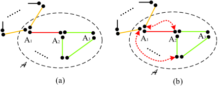
Figure 6: Schematic quantum network. (a) A general quantum network with subnetwork consisting of all parties in $\mathcal{A}$. Here, the orange lines denote entanglements shared by $\textsf{A}_{1}$ and others out of $\mathcal{A}$. The red lines denote entanglements shared by $\textsf{A}_{1}$ and others in $\mathcal{A}$. The green lines denote entanglements shared by parties (except for $\textsf{A}_{1}$) in $\mathcal{A}$. (b) Swapping two particles (red dotted lines) in $\mathcal{A}$.

Denote $\mathcal{A}_{1}$ consists of all particles $A_{1\to j}$ in Eq.(29). Denote $\mathcal{B}$ consists of all particles $A_{1\to j}$ in Eq.(28) and all particles $A_{i\to j}$ and $A_{j\to i}$ in Eq.(29). Let $SWAP(A_{i}B_{i})$ be swapping operation of two particles $A_{i}$ and $B_{i}$ defined by

$$SWAP(A_{i}B_{i})=\sum_{i}|ii\rangle\langle ii|+\sum_{i\not=j}|ij\rangle\langle ji|$$ (32)

where $A_{i}\in\mathcal{A}_{1}$ and $B_{i}\in\mathcal{B}$, as shown in Fig.S6(b). After these swapping operations, all the bipartite entangled states shared with $\mathcal{A}_{1}$ are disentangled with all the particles in $\mathcal{A}_{1}$, but re-entangled with particles in $\mathcal{B}$ if $s_{i;in}+2t_{i}\geq s_{i;out}$. This is the basic fact of entanglement swapping BBC . Hence, if $s_{i;in}+2t_{i}\geq s_{i;out}$, there is a CPTP mapping $\mathcal{E}_{\mathcal{A}}=SWAP_{\mathcal{A}}\circ\mathcal{E}_{\mathcal{A}_{1}}$ satisfying

$$\mathcal{E}_{\mathcal{A}}:\rho_{A_{1}\cdots A_{n}}\mapsto|0\rangle_{A_{1}}\langle 0|\otimes\hat{\rho}_{A_{2}\cdots{}A_{n}}$$ (33)

where $\rho_{A_{1}\cdots A_{n}}$ denotes the total state of $\mathcal{N}_{q}$, $\hat{\rho}_{A_{2}\cdots{}A_{n}}$ denotes a proper state of subnetwork consisting of $\textsf{A}_{2},\cdots,\textsf{A}_{n}$, and $SWAP_{\mathcal{A}}=\otimes_{A_{i}\in\mathcal{A}_{1}}SWAP(A_{i}B_{i})$. This means that there is a local $k$-partite mapping for transforming $\mathcal{N}_{q}$ into a disconnected network. Hence, $\mathcal{N}_{q}$ is $k$-connection biseparable state. This has completed the proof. $\Box$

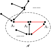
Figure 7: Schematic quantum network. A general quantum network with subnetwork consisting of all parties in $\mathcal{A}$. Here, there is a chain subnetwork shown in red lines.

Lemma 2. An $n$-partite $c$-connected quantum network $\mathcal{N}_{q}$ is $k$-connection biseparable state with $2k\geq c+1$, where the $c$-connectedness means that there are $c$ numbers of different chain subnetworks connecting each pair $(\textsf{A}_{i},\textsf{A}_{j})$ of $\mathcal{N}_{q}$.

In Lemma 2, a chain subnetwork consists of $\textsf{A}_{i_{1}},\cdots,\textsf{A}_{i_{s}}$ such that each adjacent pair share one entanglement.

Proof of Lemma 2. For any $n$-partite $c$-connected quantum network $\mathcal{N}_{q}$, there is one party ($\textsf{A}_{1}$ for example) who shares $c$ bipartite entangled states with others. Moreover, for any $c$ and $k$ there exists a $k$-partite subnetwork $\mathcal{N}_{q}^{(\mathcal{A})}$ with $\textsf{A}_{1}\in\mathcal{A}$ such that all the parties (except for $\textsf{A}_{1}$) in $\mathcal{A}$ have at least one chain subnetwork, as shown red lines in Fig.S7. This implies that

$$s_{1;in}+2t_{1}\geq 2k-2$$ (34)

where an $m$-partite chain network has $2m-2$ particles. From Lemma 1 and $s_{1;out}=c-1$ we have completed the proof. $\Box$

Author contributions

M.X.L. and S.M.F. conceived the idea. M.X.L. wrote the majority of the paper and S.M.F. reviewed this main results.

Ethics declarations

Competing interests

The authors declare no competing interests.

Additional information

Supplementary information is available for this paper online.

Correspondence and requests for materials should be addressed to M.X.

References

- (1) E. Schrödinger, Die gegenwärtige Situation in der Quantenmechanik, Naturwissenschaften 23, 807-812 (1935).
- (2) R. Horodecki, P. Horodecki, M. Horodecki, and K. Horodecki, Quantum entanglement, Rev. Mod. Phys. 81, 865 (2009).
- (3) A. Einstein, B. Podolsky, N. Rosen, Can quantum mechanical description of physical reality be considered complete? Phys. Rev. 47, 777-780 (1935).
- (4) J. S. Bell, On the Einstein-Podolsky-Rosen paradox, Phys. Rev. 1, 195 (1964).
- (5) J. F. Clauser, M. A. Horne, A. Shimony, and R. A. Holt, Proposed experiment to test local hidden-variable theories, Phys. Rev. Lett. 23, 880-884 (1969).
- (6) N. Brunner, D. Cavalcanti, S. Pironio, V. Scarani, and S. Wehner, Bell nonlocality, Rev. Mod. Phys. 86, 419 (2014).
- (7) M. X. Luo, Computationally Efficient Nonlinear Bell Inequalities for Quantum Networks, Phys. Rev. Lett. 120, 140402(2018).
- (8) A. Tavakoli, A. Pozas-Kerstjens, M. X. Luo, M.-O. Renou, Bell nonlocality in networks, Rep. Prog. Phys. 85, 056001 (2022).
- (9) H. M. Wiseman, S. J. Jones, and A. C. Doherty, Steering, Entanglement, nonlocality, and the Einstein-Podolsky-Rosen paradox, Phys. Rev. Lett. 98, 140402 (2007).
- (10) G. Svetlichny, Distinguishing three-body from two-body nonseparability by a Bell-type inequality, Phys. Rev. D 35, 3066-3069 (1987).
- (11) M. X. Luo, Fully device-independent model on quantum networks, Phys. Rev. Research 4, 013203 (2022).
- (12) D. M. Greenberger, M. A. Horne, and A. Zeilinger, in Bell’s Theorem, Quantum Theory and Conceptions of the Universe, edited by M. Kafatos (Kluwer, Dordrecht, 1989), pp. 69-72.
- (13) W. Tang, S. Yu, and C. H. Oh, Greenberger-Horne-Zeilinger Paradoxes from Qudit Graph States, Phys. Rev. Lett. 110, 100403 (2013).
- (14) Z.-H. Liu, J. Zhou, H.-X. Meng, M. Yang, Q. Li, Y. Meng, H.-Y. Su, J.-L. Chen, K. Sun, J.-S. Xu, C.-F. Li & Guang-Can Guo, Experimental test of the Greenberger-Horne-Zeilinger-type paradoxes in and beyond graph states, npj Quant. Inf. 7, 66 (2021).
- (15) M. X. Luo, S.-M. Fei, and J.-L. Chen, Blindly Verifying Partially Unknown Entanglement, iScience 25, 103972(2022).
- (16) T. Kraft, C. Ritz, N. Brunner, M. Huber, and O. Gühne, Characterizing genuine multilevel entanglement, Phys. Rev. Lett. 120, 060502 (2018).
- (17) S. Designolle, V. Srivastav, R. Uola, N. H. Valencia, W. McCutcheon, M. Malik, and N. Brunner, Genuine high-dimensional quantum steering, Phys. Rev. Lett. 126, 200404 (2021).
- (18) M. Erhard, M. Krenn & A. Zeilinger, Advances in high-dimensional quantum entanglement, Nature Rev. Phys. 2, 365-381 (2020).
- (19) M. Navascues, E. Wolfe, D. Rosset, and A. Pozas-Kerstjens, Genuine network multipartite entanglement, Phys. Rev. Lett. 125, 240505 (2020).
- (20) T. Kraft, S. Designolle, C. Ritz, N. Brunner, O. Gühne, and M. Huber, Quantum entanglement in the triangle network, arXiv:2002.03970 (2020).
- (21) M.-X. Luo, New genuine multipartite entanglement, Adv. Quantum Tech. 5, 2000123 (2021).
- (22) G. M. Quinta, R. André, A. Burchardt, K. Życzkowski, Cut-resistant links and multipartite entanglement resistant to particle loss, Phys. Rev. A 100, 062329 (2019).
- (23) T. J. Barnea, G. Pütz, J. B. Brask, N. Brunner, N. Gisin, and Y.-C. Liang, Nonlocality of W and Dicke states subject to losses, Phys. Rev. A 91, 032108 (2015).
- (24) M.-X. Luo and S.-M. Fei, Robust multipartite entanglement without entanglement breaking, Phys. Rev. Research 3, 043120 (2021).
- (25) S. Bravyi, D. Gosset and R. König, Quantum advantage with shallow circuits, Science 362, 308-311 (2018).
- (26) A. B. Watts, R. Kothari, L. Schaeffer, A. Tal, Exponential separation between shallow quantum circuits and unbounded fan-in shallow classical circuits, STOC 2019: Proceedings of the 51st Annual ACM SIGACT Symposium on Theory of Computing, 2019, pp.515-526.
- (27) M. Hillery, V. Buzek, and A. Berthiaume, Quantum secret sharing, Phys. Rev. A 59, 1829 (1999).
- (28) D. Deutsch, Quantum computational networks, Proc. Soc. Lond. A 425, 73-90 (1989).
- (29) A. Y. Vlasov, Noncommutative tori and universal sets of nonbinary quantum gates, J. Math. Phys. 43, 2959-2964 (2002).
- (30) C. H. Bennett, G. Brassard, C. Crepeau, R. Jozsa, A. Peres, and W. K. Wootters, Teleporting an unknown quantum state via dual classical and Einstein-Podolsky-Rosen channels, Phys. Rev. Lett. 70, 1895-1899 (1993).
- (31) J. Kimble, The quantum Internet, Nature 453, 1023 (2008).
- (32) M.P. Seevinck, An Inquiry into Quantum and Classical Correlations, arXiv/0811.1027v2, 2008.
- (33) W. Dür, G. Vidal, and J. I. Cirac, Three qubits can be entangled in two inequivalent ways, Phys. Rev. A 62, 062314 (2000).
- (34) R. H. Dicke, Coherence in spontaneous radiation processes, Phys. Rev. 93, 99(1954).
- (35) M. O. Renou, E. Bäumer, S. Boreiri, N. Brunner, N. Gisin, & S. Beigi, Genuine quantum nonlocality in the triangle network, Phys. Rev. Lett. 123, 140401 (2019).
- (36) H. J. Briegel and R. Raussendorf, A one-way quantum computer, Phys. Rev. Lett. 86, 5188 (2001).
- (37) M. Hein, W. Dur, J. Eisert, R. Raussendorf, M. Van den Nest and H.-J. Briegel, Entanglement in graph states and its applications, arXiv:quantph/0602096v1, 2005.
- (38) M. Horodecki, P. Horodecki, and R. Horodecki, Separability of mixed states: necessary and sufficient condition, Phys. Lett. A 223, 1 (1996).
- (39) R. F. Werner, Quantum states with Einstein-Podolsky-Rosen correlations admitting a hiddenvariable model, Phys. Rev. A 40, 4277 (1989).
- (40) Q. Y. He and M. D. Reid, Genuine multipartite Einstein-Podolsky-Rosen steering, Phys. Rev. Lett. 111, 250403 (2013).
- (41) B. D. M. Jones, I. S̆upić, R. Uola, N. Brunner, and P. Skrzypczyk, Network quantum steering, Phys. Rev. Lett. 127, 170405 (2021).