The high energy spectrum of Proxima Centauri simultaneously observed at X-ray and FUV wavelengths

The M dwarf Proxima Centauri, the Sun’s closest stellar neighbour, is known to be magnetically active and it hosts a likely Earth-like planet in its habitable zone. High-energy radiation from the host star can significantly alter planetary atmospheres in close orbits. Frequent flaring may drive radiation-induced effects such as rapid atmospheric escape and photochemical changes. Therefore, understanding the characteristics of stellar radiation by understanding the properties of the emitting plasma is of paramount importance for a proper assessment of the conditions on Proxima Centauri b and exoplanets around M dwarfs in general. This work determines the temperature structure of the coronal and transition region plasma of Proxima Centauri from simultaneous X-ray and far-ultraviolet (FUV) observations. The differential emission measure distribution (DEM) was constructed for flaring and quiescent periods by analysing optically thin X-ray and FUV emission lines. Four X-ray observations of Proxima Centauri were conducted by the LETGS instrument on board of the Chandra X-ray Observatory and four FUV observations were carried out using the STIS spectrograph on board the Hubble Space Telescope. From the X-ray light curves, we determined a variation of the quiescent count rate by a factor of two within 20% of the stellar rotation period. To obtain the DEM, 18 optically thin emission lines were analysed (12 X-ray and six FUV). The flare fluxes differ from the quiescence fluxes by factors of 4-20 (FUV) and 1-30 (X-ray). The temperature structure of the stellar corona and transition region was determined for both the quiescence and flaring state by fitting the DEM(T) with Chebyshev polynomials for a temperature range $\log$T = 4.25 - 8. Compared to quiescence, the emission measure increases during flares for temperatures below 0.3 MK (FUV dominated region) and beyond 3.6 MK (X-ray dominated region). The reconstructed DEM shape provides acceptable line flux predictions compared to the measured values. Using the DEM we provide synthetic spectra at 1-1700 Å, which may be considered as representative for the high-energy irradiation of Proxima Cen b during quiescent and flare periods. In future work these values can be used for planet atmosphere calculations which will ultimately provide information about how habitable Proxima Centauri b is.

1 Introduction

At a distance of 1.3 pc (Gaia Collaboration 2018), the red dwarf Proxima Centauri, as the third member of the $\alpha$ Centauri system, is the Sun’s closest stellar neighbour. It has a spectral type of dM5.5 (Bessell 1991), corresponding to an effective temperature of 3040 K (Ségransan et al. 2003). The mass of Proxima Centauri is 0.12 $M_{\odot}$, its radius is 0.15 $R_{\odot}$ (Ségransan et al. 2003), and its luminosity is 0.0015 $L_{\odot}$ (Doyle & Butler 1990). It is known to be magnetically active, as was revealed for example in the X-ray regime by the Einstein satellite (Haisch et al. 1980). Despite its $\approx 50$ times smaller surface area compared to the Sun, Proxima Centauri’s quiescent X-ray luminosity $L_{X}\approx(0.4-1.6)\cdot 10^{27}$ erg s^-1 is similar to the Sun’s (Haisch et al. 1990). During flares, bolometric energies of up to $\approx 10^{33.5}$ erg are released by the star (Howard et al. 2018), covering wavelengths from the X-ray to millimetre range (MacGregor et al. 2021). Nevertheless, Proxima Centauri exhibits only a moderate magnetic field of B$f\approx\,600$ G (Reiners & Basri 2008; Klein et al. 2021), which is in line with its long rotation period of about 83 days (Benedict et al. 1998).

Proxima Centauri garnered increased interest, when Anglada-Escudé et al. (2016) announced the existence of a small planet (Proxima Centauri b) with a minimum mass of 1.3 $M_{\oplus}$, that is orbiting in the star’s habitable zone at a distance of 0.05 AU (P$=11.2$ days). Questions began to rise as to whether the intrinsic planetary properties as well as the stellar environment of Proxima Centauri allow for a habitable planetary climate. In particular, the incident stellar radiation at short wavelengths – which is X-ray, ¡100 Å  and extreme ultraviolet (EUV), 100-912 Å  – can have adverse effects on the atmosphere of the planet at such close orbital distances, especially during flares, when it is usually drastically increased. For example, high-energy radiation can lead to the heating and ionisation of atmospheric gas and, in consequence, to thermal atmospheric escape (García Muñoz 2007; Murray-Clay et al. 2009; Koskinen et al. 2010; Salz et al. 2016). At longer wavelengths – far ultraviolet (FUV), 912-1700 $\AA$  – stellar radiation potentially induces non-thermal chemistry (i.e. photo-chemistry), which can cause the loss of oceans and the build-up of abiotic-produced O₂ and O₃ (Luger & Barnes 2015; Loyd et al. 2018). In contrast, ozone layers may be totally eroded by proton events (Tilley et al. 2019).

Stellar X-rays and ultraviolet (UV) photons are produced by the hot plasma in stellar coronae and transition regions with a strong correlation of X-ray luminosity to the magnetic field (Reiners 2012) and to the coronal temperature (Güdel 2004). X-ray and UV radiation peaks during flares, which are the result of magnetic re-connection at large atmospheric heights (Benz 2017). During such events, coronal temperatures reach values of up to 10 MK and more. Since flare events are unpredictable and cover only a fraction of the star’s surface, the plasma associated with flares spans a large range in temperature, at least from $10^{4}$ to $10^{7}$ K (Benz 2017; Howard et al. 2020). However, X-ray and FUV telescopes cannot spatially resolve the surface of a star other than the Sun, and therefore spectroscopic measurements average information from multiple different plasma features. By determining the differential emission measure (DEM) through spectroscopic analysis of X-ray and FUV emission lines, the temperature structure of the emitting object can be reconstructed, which we performed here for partially simultaneous X-ray data taken by Chandra/LETGS and FUV data taken by Hubble/STIS. Since several flares occurred during the observations, we took the opportunity to construct separate DEMs for flaring and the quasi-quiescent state of Proxima Centauri.

Our paper is structured as follows. In Sect. 2, we give a short theoretical introduction to the concept of the differential emission measure. In Sect. 3, the observation information is listed. Sect. 4 covers the timing as well as the spectral analysis of the X-ray and FUV data, while the DEM fitting is described in Sect. 5. Section 6 contains our results and a discussion of them, while Sect. 7 presents a summary and conclusion.

2 Differential emission measure

Due to the mostly inhomogeneous nature of the stellar corona and transition region, measured fluxes represent – in reality – the integrated emission of a large number of individual features of the spatially unresolved, outer stellar atmosphere. The combined effect of these different features, which are unknown to the observer, can be parameterised by the DEM distribution function $\xi(T)$.

2.1 Computation of the DEM

The DEM is a physical quantity that is related to the product of electron density $n_{e}$ and ion density $n_{ion}$, as well as the infinitesimal volume of plasma $dV$ associated with an infinitesimal range of temperature $1/dT$ (Landi & Chiuderi Drago 2008). We further assume $n_{ion}\approx n_{H}\approx n_{e}$, with $n_{H}$ being the density of ionised hydrogen, and used the following for the DEM:

$$\xi(T)=n_{e}^{2}\frac{dV}{dT}\,,$$ (1)

with units in $\textrm{cm}^{-3}\textrm{K}^{-1}$. Another quantity often used in the literature is the volume emission measure ($EM$) defined as

$$EM=\int n_{e}n_{H}dV$$ (2)

with units in $\textrm{cm}^{-3}$. The DEM and the EM are related through

$$EM_{\Delta T}(T)=\int_{T-\frac{\Delta T}{2}}^{T+\frac{\Delta T}{2}}\xi(T)dT\,.$$ (3)

The DEM is an established description for modelling plasma structures (see, e.g. Schmitt & Ness 2004; Liefke et al. 2008; Duvvuri et al. 2021). It can be determined in many ways, almost all of which make use of emission lines in the FUV and X-ray ranges (Landi & Chiuderi Drago 2008). When assuming the plasma to be optically thin and in collisional ionisation equilibrium, the observed emission line fluxes can be expressed as

$$F(\lambda)=\frac{1}{4\pi d^{2}}\int_{V}G(T,\lambda,N_{e})\;\xi(T)\;dT,$$ (4)

where $d$ is the distance between the observer and the plasma, and $G(T,\lambda,N_{e})$ is the contribution function at wavelength $\lambda$ of all spectral lines. The contribution function, which is strongly dependent on the plasma temperature $T$, is determined by the atomic parameters of the spectral line and can be calculated using atomic databases.

Equation 4 constitutes a Fredholm equation of the first kind, and the inversion of which yields the DEM function $\xi(T)$. This type of integral inversion is ill-conditioned with no unique solution for $\xi(T)$ unless one imposes additional constraints (Güdel 2004). A formal discussion on this issue can be found in Craig & Brown (1976). For the constraints applied here, readers can refer to Sect. 2.2.

The basic integral equation can be solved numerically by replacing the integral operator $G(T,\lambda,N_{e})$ with a matrix operator. This approach is useful since the flux $F(\lambda)$ is only measured at a finite number of points $\lambda_{m}$, and it is therefore only possible to solve Eq. 4 for a discrete approximation to $\xi(T)$. The matrix approximation may be obtained by discretising the temperature into $n$ bins, so that

$$F(\lambda_{m})=\frac{1}{4\pi d^{2}}\sum_{k=1}^{n}G(T_{k},\lambda_{m})\xi(T_{k}).$$ (5)

Written in matrix form, the solution of $\@vec{\xi}$ is now obtained by the inversion of $\@tens{G}$. This may be done in a variety of ways, one of which being the expansion of $\xi(T)$ in a series of orthogonal polynomials. Here we opted for Chebyshev polynomials due to their favourable boundary conditions.

2.2 Applied constraints to the DEM

For the determination of the DEM, some constraints need to be imposed (Schmitt & Ness 2004), with the most trivial one being

$$\xi(T)\geq 0.$$ (6)

The second constraint is

$$\xi(T_{max})=0,$$ (7)

assuming a maximum temperature $T_{max}$ above which no emission measure is present. Finally, in the absence of any plausible physical model, the distribution function $\xi(T)$ can be approximated by the sum of $N$ orthogonal polynomials (Schmitt & Ness 2004):

$$\xi(T)=\sum_{i=0}^{N}a_{i}Ch_{i}(x),$$ (8)

with $Ch_{i}(x)$ being Chebyshev polynomials of order $i$ and the dimensionless temperature variable $x$ defined in the closed interval [0,1]:

$$x(T)=\frac{\text{log}(T)-\text{log}(T_{min})}{\text{log}(T_{max})-\text{log}(T_{min})}.$$ (9)

We determined the coefficients $a_{i}$ by a fit to the data. The used boundary conditions are

$$Ch_{2i}(0)=(-1)^{i}\qquad Ch_{2i+1}(0)=0\qquad Ch_{i}(1)=1.$$ (10)

Combining the third boundary condition with $\xi(1)=0$ (equivalent to Eq. 7), the following relation was obtained for the Chebyshev coefficients $a_{i}$:

$$\sum_{i=0}^{N}a_{i}=0.$$ (11)

Therefore, the number of independent coefficients $a_{i}$ is $N$ and the coefficient $a_{0}$ can be written as

$$a_{0}=-\sum_{i=1}^{N}a_{i}.$$ (12)

3 Simultaneous observations and data reduction

We obtained X-ray and FUV observations of Proxima Centauri in 2017 with the Chandra and Hubble Space Telescope (HST), respectively, with the HST data having been obtained strictly simultaneously with the third out of the four X-ray observations. This third observation is also covered by Astrosat X-ray data and was analysed with a focus on the timing and multi-wavelength behaviour by Lalitha et al. (2020). Here the focus is on the construction of the DEM, and the light curves were mainly used to identify flaring and quiescent episodes.

3.1 FUV observations and data reduction

HST observed Proxima Centauri on 31 May 2017 during four consecutive orbits (Prop. ID: 14860); for observation time details, readers can refer to Table 1. The combined exposure time of all four measurements was 12.28 ks. All observations were performed with the STIS/FUV MAMA detector (Ward-Duong et al. 2021). In combination with the echelle grating E140M, the instrument provides spectra at a resolving power of $\sim 40\,000$ in the wavelength range 1140-1710 Å. The aperture defining slits covered an area of 0.2$\times$0.2 arcsec on the sky as recommended for point sources. All data were taken in TIME-TAG mode, allowing us to construct light curves in spectral windows which were defined a posteriori. Data were downloaded from the Hubble Legacy Archive and were reduced with calstis.

3.2 X-ray observations and data reduction

The Chandra X-ray observatory (Weisskopf et al. 2002) observed Proxima Centauri between 15 May and 3 June 2017 four times for a total of 175 ks (PI: Predehl, Prop. ID: 18200754). For details on the observation times, readers can refer to Table 1. The combined exposure time of all four measurements was 165.93 ks. All observations were performed with the Low Energy Transmission Grating Spectrometer (LETGS), which operates by using the Low Energy Transmission Grating (LETG) in conjunction with the High Resolution Camera (HRC-S). LETGS provides high-resolution spectroscopy $(\lambda/\Delta\lambda>1,000)$ between 50 and 160 Å  and $\lambda/\Delta\lambda\approx 20\cdot\lambda$ at shorter wavelengths (3-50 Å). The full LETGS wavelength range is 1.2 - 175 Å  (0.07 - 10 keV). The first order effective area varies between 1-25 cm². All X-ray data used in this study were downloaded from the Chandra Data Archive and reduced using CIAO 4.11. For standard processing and calibration, CALDB 4.8.3 was used.

Table 1: Chandra LETGS and Hubble STIS observation times

Start date	Obs. ID	Dur. [ks]
Chandra
2017-05-15 23:27:56	20073	40
2017-05-18 09:19:55	20080	52
2017-05-31 16:24:33	19708	45
2017-06-03 04:44:16	20084	30
Hubble
2017-05-31 21:19:36	201010	2.5
2017-05-31 22:32:21	201020	3.2
2017-06-01 00:07:21	201030	3.2
2017-06-01 01:43:12	201040	3.2

4 Light curve analysis

The following section provides an analysis of the X-ray and FUV light curves obtained from the Chandra LETGS and Hubble STIS observations. The main focus lies on the identification of flaring and quiescent periods for the construction of a quiescent and a flaring DEM.

We classify Proxima Centauri’s activity into three different states, namely flaring, quiescent, and intermediate state. Quiescent intervals are characterised by low stochastic variability around a mean count rate. This quiescent count rate can change over time, for example if the filling factor of hot material changes. The flare identification process can be formalised, but ultimately remains subjective, for example by setting threshold values. Given the low number of flares in our case, the following criteria were applied manually: The flaring periods were selected by identifying instantaneous (in seconds to minutes) increases in the photon count rate by a minimum factor of three times the quiescent rate. The end of each flaring period was assigned when the count rate had decreased to approximately the quiescent count rate. The remaining parts of the light curve – which could not be assigned to quiescent or flaring state – were classified as being in an intermediate state. For the FUV data, the two intermediate time intervals seem to be located at the end of decay phases of flares, with one occurring before the observations started and the other being a secondary flare. In the X-ray data, we identified a lot more intermediate state time intervals, which are characterised by being above the quiescent level, giving evidence of higher activity without a connection to clear flaring signatures. To make sure that we are only dealing with the bona fide quiescent and flaring state for the DEM construction, these intermediate intervals are excluded from the following analysis. Flaring periods are marked in red in Figs. 1 and 2 in the Hubble FUV and Chandra X-ray light curves, while phases of the quiescent state are marked in green. Intermediate-type intervals are not marked. Flares are also numbered by roman numerals for better reference.

4.1 FUV light curves

The FUV light curves were extracted from the STIS/FUV-MAMA detector using the python module lightcurve and an integration range from 1100 to 1700 Å. They are shown in Fig. 1. They display the background-subtracted photon count rates with a temporal binning of 1 s. The FUV light curves show their typical behaviour of a well-defined quiescent state, with the exception of pronounced flares.

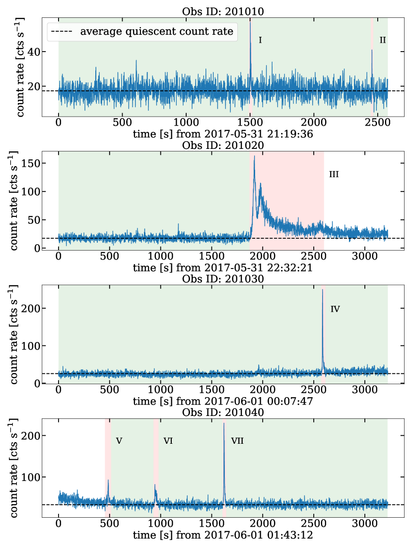
Figure 1: Background-subtracted FUV light curves of Hubble/STIS observations (blue line). The red shaded areas indicate flares, which are labelled with roman numerals. The green shaded areas show quiescent time intervals. The non-shaded intervals are classified as being in an intermediate state. The dashed horizontal line indicates the average quiescent count rate in the individual observation runs.

The different observations for the first two runs (201010 and 201020) display an average quiescent count rate of 17.32 cts/s. In the third observation (201030), we find a higher average quiescent count rate of 25.59 cts/s, while the last observation (201040) has the highest quiescent count rate with 33.12 cts/s. The higher average quiescent count rates of the latter two observations can be explained by the higher overall activity state of Proxima Centauri during that time, indicated by more frequent flaring and by the continuous X-ray light curve displaying higher count rate levels, as well as more variability during this time interval (see Fig. 2 for comparison). The quiescent time intervals of all four observations add up to 10.2 ks with an average count rate of 23.96 cts/s, which corresponds to $L_{FUV,qu}=1.4\cdot 10^{26}$ erg s^-1.

Table 2: Flare properties of FUV and X-ray flares.

flare	length	max.	total
		count rate	counts
	[s]	[cts/s]	[cts]
FUV I	30	57	655
FUV II	27	45	361
FUV III	729	163	33094
FUV IV	41	251	2516
FUV V	47	97	2648
FUV VI	47	87	2277
FUV VII	43	232	2574
X-ray I	3000	0.79	1508
X-ray II	880	0.71	501
X-ray III	850	1.04	438
X-ray IV	1100	1.04	431
X-ray V	1220	0.36	288

The FUV light curve displays seven flare intervals as designated in Fig. 1. Their individual duration, maximum count rate, and total flare counts are listed in Table 2. The total combined flaring time is 964 s, with Flare III contributing $\sim$75 $\%$ of that time and also dominating the total flare counts. Moreover, the morphology of Flare III is different since it is the only flare with a notable duration and also as it exhibits a secondary flare maximum. This implies that the flare also dominates the DEM construction for the flaring time interval. During flares, the photon count rate increases by factors of 2.4 to 10.5. The average count rate increase for the identified flares is a factor of 5.5 for the flare maximum, while the average flare luminosity is $L_{UV,fl}=7.7\cdot 10^{26}$ erg s^-1.

4.2 X-ray light curves

The background-subtracted X-ray light curves extracted from the zeroth order of LETGS are shown in Fig. 2. The temporal binning is 100 s. During all four observations, the X-ray activity level varies even on short time scales also exhibiting some sort of flickering outside the flares, which is a rather typical behaviour of M dwarfs (Robrade & Schmitt 2005). Examples of flickering can be found in the time intervals classified as intermediate.

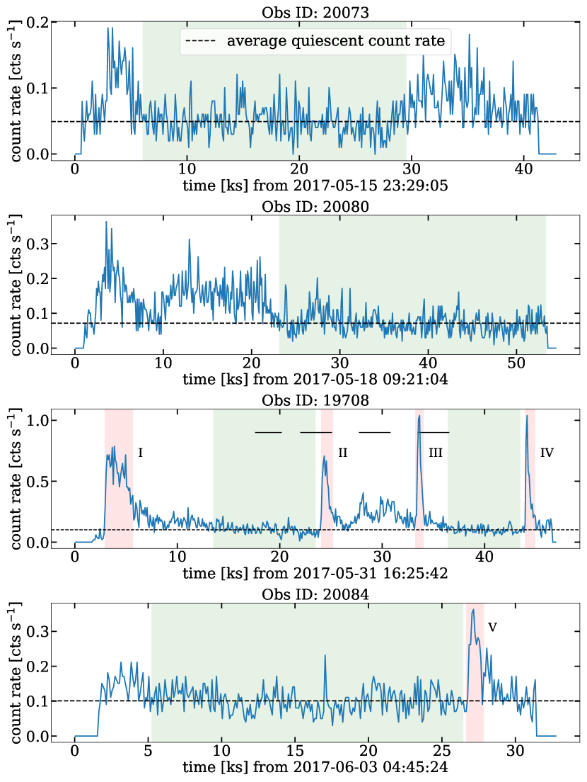
Figure 2: Background-subtracted X-ray light curves of Chandra/LETGS observations (blue line) constructed from the zeroth order. Flare and quiescent periods are shown in red and green shaded areas, respectively. Flares are labelled by roman numerals and the dashed horizontal lines indicate the quiescent average count rate for each observation. The black horizontal bars mark the time intervals of each of the four FUV observations.

Observation 20073 displays mostly quiescent as well as slightly enhanced emission. The quiescent period lasts for 23.5 ks and has an average count rate of 0.049$\pm$0.002 cts/s. The light curve of observation 20080 shows a similar picture: After a period of small variability with no clear indications of a flare, a quiescent time interval follows. This lasts for 30.2 ks with an average 0.072$\pm$0.002 cts/s. The light curve of observation 19708 displays two time intervals in which Proxima Centauri is quiescent. Overall they last for 17 ks with a combined average count rate of 0.102$\pm$0.003 cts/s. Observation 20084 displays one long period of quiescence that lasts for 21.2 ks with an average count rate of 0.101$\pm$0.002 cts/s. The quiescent time intervals of all four observations add up to 91.9 ks with a total average count rate of 0.077 cts/s, which equates to $L_{X,qu}=6.6\cdot 10^{26}$ erg s^-1, assuming the DEM peaks at $\log T=6.6$ (the DEM is calculated in Sect. 6, see Fig. 7) and using an APEC model. This implies a rather low activity state of Proxima Centauri during the observations as quiescent X-ray observations range from 0.4 to 1.6 $\cdot 10^{27}$ erg s^-1 (Haisch et al. 1990).

Nevertheless, the quiescent count rates vary by a factor of 2 within a span of 17 days between observations. Since this is only 20 $\%$ of the stellar rotational period, either a more active region has rotated into view or the variation is due to the stochastic nature of stellar activity.

The X-ray light curve displays five flare events as marked in Fig. 2 with their flaring properties given in Table 2. The total combined flaring time is 7.03 ks, with Flare I dominating in time and total counts. This flare is not covered by the FUV observations.

During flares, the photon count rate increases by factors of 5 to 13.5. On average, the count rate increases by a factor of 10 during flare maxima. The average flare luminosity is $L_{X,fl}=6.7\cdot 10^{27}$ erg s^-1.

4.3 Comparison of FUV and X-ray light curve

Figure 3 shows both the Chandra and Hubble light curves in the overlapping time interval. It can be noted that often distinct flares in the FUV wavelength range do not need to have marked counterparts in the X-ray regime, as can be seen for FUV flare IV which occurs during X-ray flickering, without a larger flare associated with it or FUV flare VII, which is not even accompanied by X-ray flickering. This behaviour is possibly caused by the better binning of the FUV data compared to the X-ray data and the shortness of the FUV flares. Both of which lead to a veiling of the event in X-ray.

X-ray flare II is preceded by FUV flare III, which is consistent with the Neupert effect because integration of the FUV light curve leads to a close resemblance of the X-ray flux increase at the start of the flare until the X-ray peak is reached. X-ray flare III is associated with the onset of the fourth Hubble observation, which shows a decrease in count rate, also suggesting a preceding FUV flare event of an unknown amplitude for X-ray flare III.

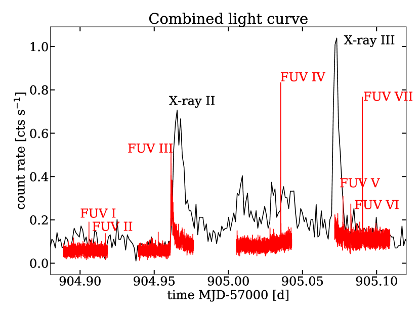
Figure 3: Combined light curve of Chandra (black) and Hubble (red) for the overlapping time period. Flare events are marked by their assigned roman numerals for X-ray flares in black and for FUV flares in red. The FUV light curve is scaled for convenience.

5 Construction of the DEM

With the quiescent and flaring periods identified in the previous step, spectra were generated by combining all flaring as well as quiescent periods for the FUV and X-ray observations. In Fig. 4 we show the thusly constructed quiescent and flaring spectra of our FUV data. From these different spectra, line fluxes were obtained by fitting Voigt profiles to the emission line profiles in the FUV range and by integrating the spectrum for the Chandra X-ray lines because of their lower signal-to-noise ratio. Specifically, for the X-ray lines, the calculation was performed by summing up observed photon counts within a 2$\sigma$ range, where $\sigma$ = 0.036 $\AA$ was estimated from a Gaussian fit to the strong O VIII line at 18.97 Å. For each line, instrumental background and continuum were also accounted for with the background counts calculated in the wavelength intervals ranging from 3$\sigma$ to 9$\sigma$ of each line.

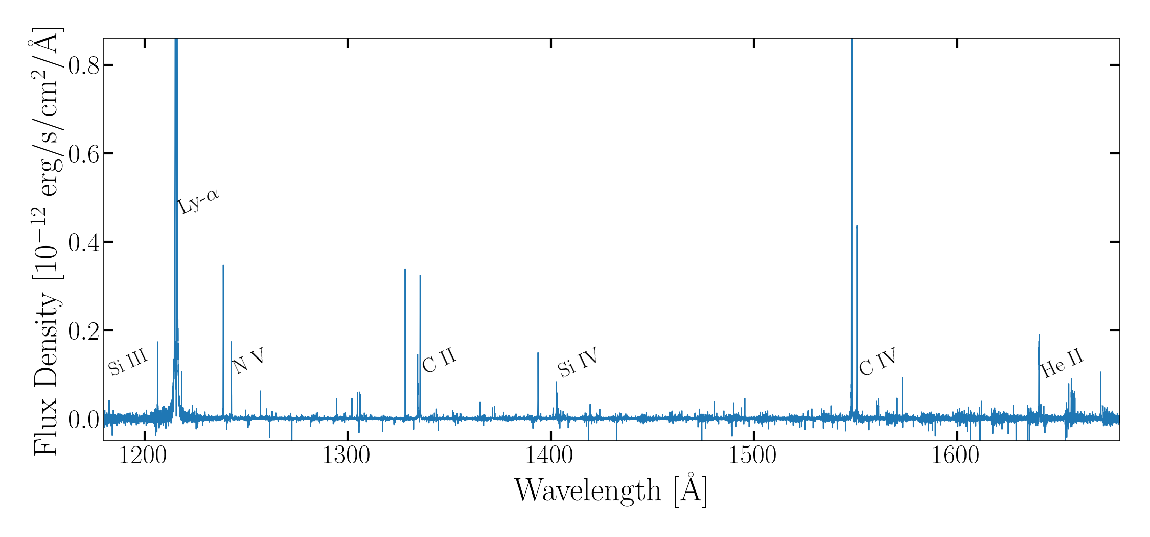
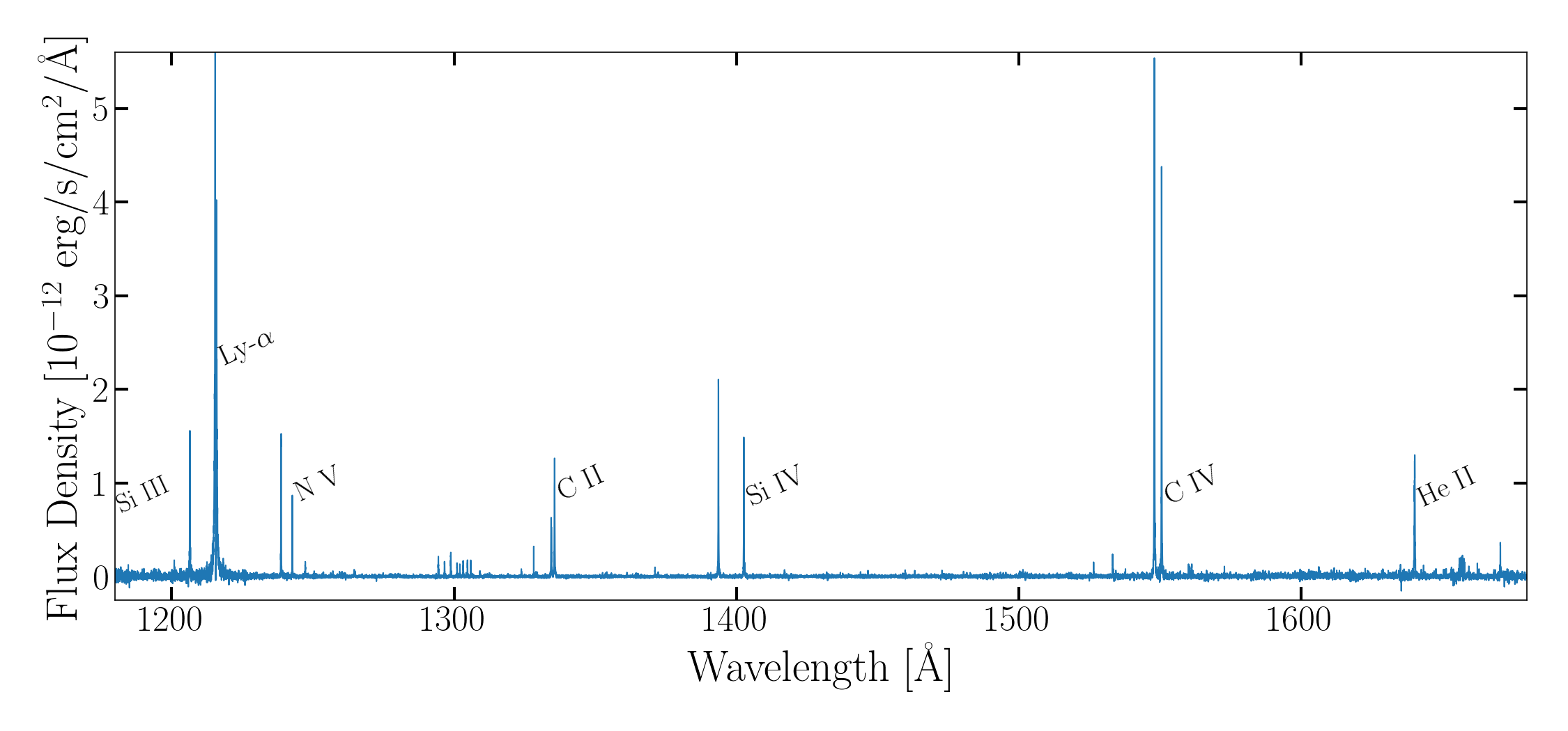
Figure 4: Hubble FUV spectra extracted from the quiescent (top) and the flaring state (bottom). The most significant lines are labelled, even if they are not used for the further DEM analysis.

To give an impression of the quality of the X-ray spectra, we show the X-ray spectrum of the whole exposure (166 ks) in Fig. 5. The spectrum is in agreement with a relative low emission measure at low temperatures generating X-ray emission; this can be seen for example from the absent Fe ix and Fe x lines at 171 and 174 Å, which have peak formation temperatures at $\log$T = 5.9 and 6.1, respectively. We caution though that these two lines may also be undetectable due to the low effective area of the instrument at these wavelengths ($\approx 1\,$cm², see also Sect. 6.2 for a more detailed discussion).

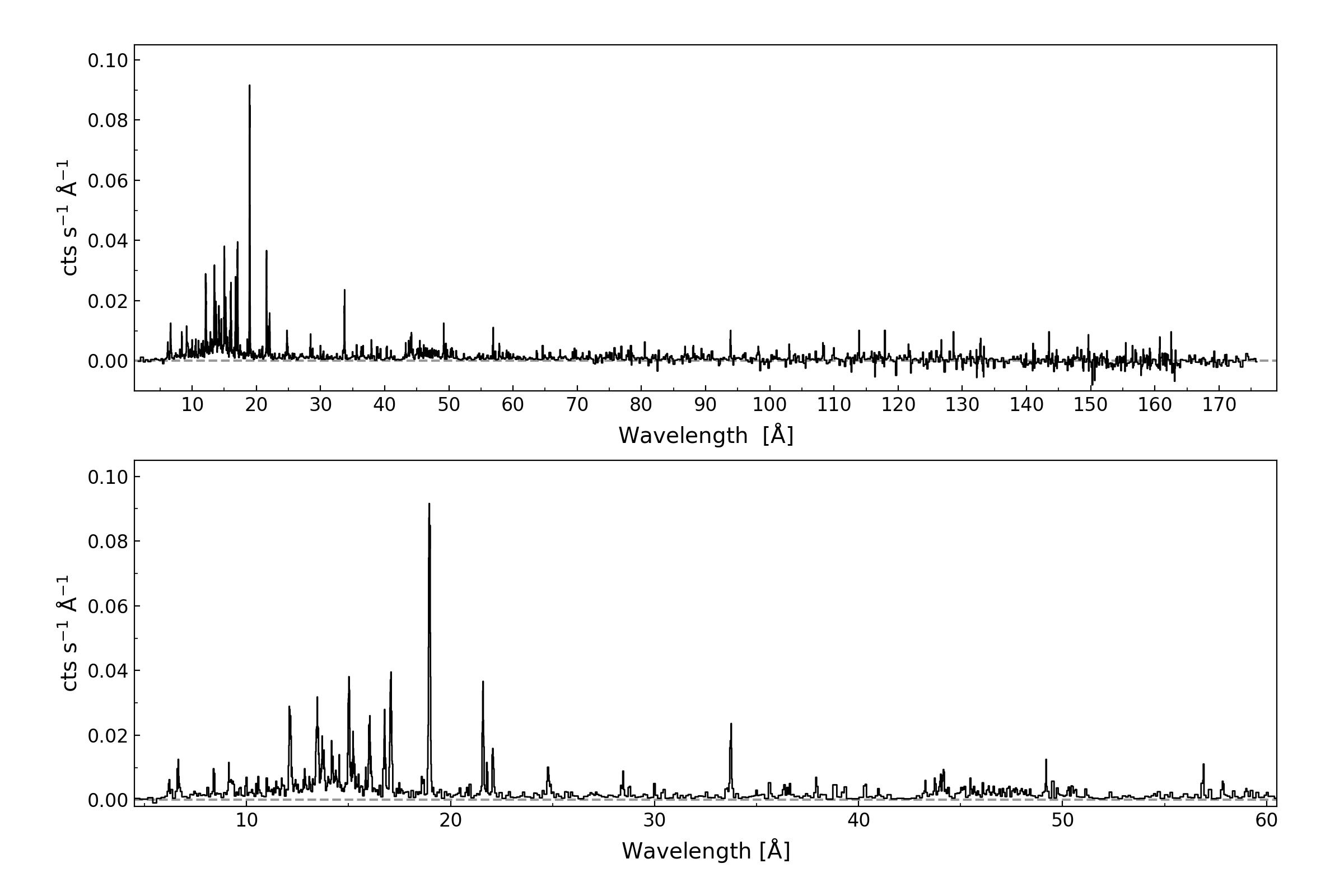
Figure 5: Chandra X-ray spectrum for the whole observation (166 ks) binned to minimum of abs(20) counts per bin (top). The zoom (bottom) shows the wavelength range used here.

The flux values for 25 emission lines in the X-ray regime, which include ions of Si, Mg, Ne, Fe, O, N, C, and Ni, were calculated for flare and quiescence periods. In the FUV, we found a total of 16 emission lines, which include ions of Si, N, C, and He. Unfortunately the seven He lines are all blended so severely with wavelengths between 1640.33 and 1640.53 Å  that we could not disentangle the lines. Moreover, the line formation process for He ii is not expected to be well-described by our assumption of collisionally dominated plasma. This led us to exclude these lines from any further analysis.

Also, the quiescent FUV spectrum shows some excess around the Fe XXI line at 1354 Å. However, since this part of the spectrum is very noisy and the photon excess has a distinctly different shape than other lines (being much broader), we did not consider this Fe XXI line in our analysis. We note, nevertheless, that interpreting the excess as a genuine line flux would be roughly compatible with other detected X-ray lines having peak formation temperatures in the same temperature range.

From this preliminary set of emission lines, we identified suitable lines for the DEM fitting. For the FUV range, all line fluxes were measured with higher precision compared to the X-ray line fluxes as can be seen in Fig. 6. Unfortunately, two of the lines show signs of self-absorption implying that these lines are not optically thin. We therefore decided to exclude them from the further analysis. The two lines are a C II line, whose line shape exhibits a distinct double peak and a Si III line, which also shows signs of self-absorption during the flare. Moreover, we selected 15 X-ray emission lines with significant flux ($>3\sigma_{flux}),$ either in the quiescent or flaring spectra. From these, we excluded three lines: one O VIII line at 16.0 Å, which is a blend with another O VIII line and a strong line of Fe XVIII. Moreover, we excluded one O VII line at 22.1 Å and one Ne IX line at 13.7 Å, which both are density sensitive, since they both are the forbidden line component of a He-like triplet (Ness et al. 2002). Thus we were left with 12 X-ray lines for the DEM fitting, using the same set of lines for a flaring and quiescent state, though some line fluxes are consistent with zero in one of the two states. The measured properties of these lines can be found in the appendix in Table 4 for the X-ray data and in Table 5 for the FUV lines.

The total line fluxes are shown in Fig. 6, where they are plotted against their peak formation temperatures as listed in the APED database (Smith et al. 2001). The peak formation temperature is the temperature at which the emissivity of an atomic line is maximal.

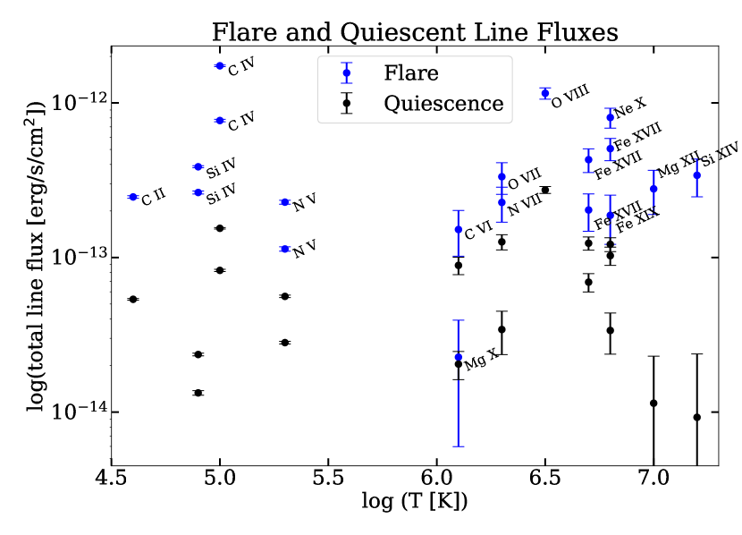
Figure 6: Total line fluxes of all X-ray and FUV emission lines plotted versus their peak formation temperatures during flares (blue) and quiescence (black). Both wavelength regimes are clearly distinct, with the FUV lines being below 10^5.5 K and the X-ray lines being above 10^6.0 K.

A clear distinction between FUV and X-ray lines can be seen in Fig. 6. The FUV lines are most efficiently produced at temperatures between $\log$ T = 4.6 - 5.3 (40 000 - 200 000 K), while the X-ray lines are emitted in the temperature range $\log$ T = 6.1 - 7.2 (1.2 - 15.8 MK). In our data, no lines that formed in the temperature range $\log$ T = 5.4 - 6.0 (250 000 - 1 000 000 K) were measured. Such lines would be emitted mostly in the extreme ultraviolet (EUV, 100 - 1200 Å), of which only a fraction is covered by Chandra and being hampered by low sensitivity in this wavelength region. We therefore chose the definition range for our DEM calculations to start from $\log$(T_min) = 4.25 since our data are largely insensitive to cooler plasma. While this lower temperature end comes without any further constraints, we set $\log$(T${}_{max})=8.0$, with the constraint that the DEM(T_max)=0, as detailed in Sect. 2.2, since we expect no relevant emission above this temperature.

The strongest emission line in the FUV in our data is C IV. The strongest X-ray lines are O VIII, O VII, and Fe XVII. The differences in the errors of X-ray and FUV fluxes are caused by the lower sensitivity of Chandra in comparison to Hubble/STIS, which leads to comparably few counts in the X-ray range resulting in larger statistical errors.

For the construction of the DEM from this line set, in principle, the solution with the lowest order polynomial which still provides an acceptable fit to the data should be chosen. In the case of this study, polynomials of order five are used for the quiescent data and those of order six for flaring data. The fit of the quiescent DEM function was conducted while varying the elemental abundances of the coronal plasma with the Fe abundance fixed to one. For the flaring DEM fit, we first fixed the abundances to the ones obtained for the quiescent DEM and fitted the Chebyshev polynomial coefficients, then in a second step we fixed the coefficients and fitted the abundances. Further we calculated errors for the DEM fit as follows: To calculate the errors of the Chebyshev polynomial coefficients, we kept the abundances fixed and chose random flux values within the obtained errors and we re-calculated the fit 100 times. To calculate the errors of the abundances, we in turn kept the coefficients of the Chebyshev polynomial fixed. Although we chose this method for its computational robustness, we caution, nevertheless, that changes in the DEM or abundances may compensate for each other and still yield similar fluxes. Therefore, this method may underestimate the errors.

6 Results

6.1 Elemental abundances

The best-fit abundances obtained from the DEM fitting process described in Sect. 5 are listed in Tab. 3 with respect to solar abundance as given by Anders & Grevesse (1989). Although we derived abundances that are in detail different from those by Güdel et al. (2004) and Fuhrmeister et al. (2011), our results are overall similar. For an active star such as Proxima Centauri, an inverse first ionisation potential (FIP) effect-like abundance pattern is expected, that is elements of low FIP are depleted compared to elements of high FIP (Audard et al. 2003). While Fuhrmeister et al. (2011) found a tentative inverse FIP pattern during the quiescence state for Proxima Centauri, Güdel et al. (2004) found a rather flat abundance pattern close to solar photospheric values. Our abundance pattern is inconclusive concerning a FIP or inverse FIP effect, but it is also relatively close to solar photospheric values. This may be explained by the rather inactive state of Proxima Centauri during our observations, as seen by the low X-ray and FUV fluxes (as discussed in Sects. 4.1 and 4.2). Also, most of our flaring abundances are quite similar to the quiescent values, which is as expected since the observed flaring activity does not include large flares.

Güdel et al. (2004) also used the solar abundances by Anders & Grevesse (1989), except for Fe, where they used Grevesse & Sauval (1999). Here, we compare our abundance analysis to their results in more detail. We recalculated their abundancy ratios to the abundancy stated by Anders & Grevesse (1989) and found no difference for the given accuracy, except for Fe/H=0.50 instead of their original value of 0.51. Therefore, we provide their abundance ratios in Table 3. We opted for a normalisation with respect to Fe since the largest number of used lines in the X-ray regime originate from Fe. Using this normalisation to an Fe abundance of 1.0, all given values also represent abundance ratios relative to Fe. Thus the abundance ratios are in agreement with those from Güdel et al. (2004), except for O/Fe, which is higher in our data.

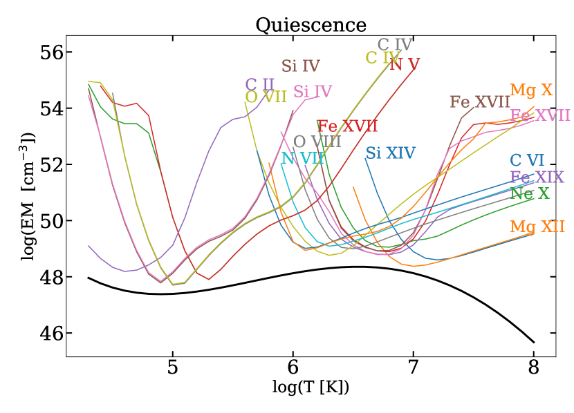
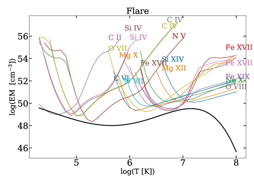
Figure 7: Discretised emission measure distribution of Proxima Centauri (black line) during quiescence (top) and during combined flare periods (bottom). As assumed by the fitting model, the emission measure vanishes at high temperatures. Coloured lines represent the observed line fluxes divided by their contribution function. Their minima are at the peak formation temperatures of the respective line.

Table 3: Elemental abundances relative to solar photospheric values.

Ion	Relative Abundance		Güdel et al. (2004)
	Quiescence	Flare	Quiescence
C/Fe	1.45 $\pm$ 0.31	1.07$\pm$ 0.18	1.9$\pm$0.7
N/Fe	1.19 $\pm$ 0.23	1.77$\pm$ 0.47	1.5$\pm$0.6
O/Fe	1.44 $\pm$ 0.33	1.23$\pm$ 0.30	0.6$\pm$0.2
Ne/Fe	2.06 $\pm$ 0.61	1.34$\pm$ 0.36	1.6$\pm$0.6
Mg/Fe	3.5 $\pm$ 0.46	1.54$\pm$ 0.91	2.1$\pm$0.9
Si/Fe	1.67 $\pm$0.75	1.99$\pm$ 0.21	2.1$\pm$0.8
Fe/H	1.0	1.0	0.50$\pm$0.15

6.2 DEM

The results of the DEM fitting process are shown in Fig. 7 for quiescence (top panel) and the flaring (bottom panel) period, where the black line represents the discretised emission measure of Proxima Centauri with a logarithmic binning of $\text{log}(T_{i+1})-\text{log}(T_{i})=\text{log}(T_{i+1}/T_{i})=0.1$. The coloured lines represent the measured line fluxes of all emission lines that were selected for the DEM fitting, divided by their contribution function. These curves are sharply peaked in temperature with their minima being at the respective peak formation temperature of the emitting line. Only some curves, especially of X-ray lines (e.g. O VIII), are somewhat flat towards higher temperatures. These irregularities are caused by the calculation of the contribution function with the help of atomic databases. If ions are listed in the database at similar wavelengths to the observed emission line, they contribute to the emission depending on their theoretical relative flux, but often at different temperatures. Since their contribution is negligible in comparison to the observed lines, this behaviour did not compromise the fitting of the DEM curves.

The binned flare EM peaks around $\log$ T = 7.2 (15.8 MK), while a smaller secondary peak can be seen at the low temperature end, which indicates enhanced emission of UV photons during flares. The quiescence EM expectedly peaks at a lower plasma temperature, $\log$ T = 6.3 (2.0 MK), which is still within the X-ray dominated temperature range. Beyond a local broad minimum of the quiescence EM around $\log$ T = 4.8 (63 000 K), the EM increases again to the low temperature end. These results roughly match the calculations of Güdel et al. (2004), who observed Proxima Centauri in X-rays using the X-ray satellite XMM-Newton and found the EM distribution during low-level episodes to be dominated by plasma at $\log$ T = 6.48 (3.0 MK). For an observed flare, they found the EM to peak at $\log$ T = 7.18 - 7.30 (15.1 - 20 MK). Since they lacked FUV data, their EM fitting starts at 1 MK.

In Fig. 8 the DEM distributions during flares and quiescence are shown together with the obtained errors. The flare-DEM exhibits significantly higher values than the quiescence-DEM for nearly every temperature besides the temperature region around $\log$ T=5.8. Those temperatures are not well-constrained in our data because lines with formation temperatures in that range are neither significantly detected in the quiescent nor flare state. Although the formation temperature of the Fe IX line at 171 Å  and the Fe X line at 174 Å  is in the considered regime, these lines fall in a detector region with very poor sensitivity (effective area of $\approx 1\,$cm²) and a high background, making meaningful conclusions challenging. In any case, their nominal upper limits are in contradiction with the predicted fluxes based on the reconstructed DEM and they would require somewhat lower (D)EM values around roughly $\log$ T=5.8. Abundance effects are likely insufficient to explain this discrepancy between the “low temperature” Fe lines and the DEM prediction because Fe lines with a higher formation temperature are generally compatible with lines of other ions. Therefore, any DEM respecting the low temperature Fe-line upper limits would greatly underestimate several other, clearly detected lines (chiefly C vi and O vii), so that the inclusion of these low temperature Fe lines into the fit has only a marginal effect on the resulting DEM. Therefore, we conclude that the DEM around $\log T\approx 5.8$ may be slightly, but not greatly, lower than what was reconstructed.

The ratio between flare and quiescent fluxes (see Fig. 10) as a function of the peak formation temperature indicates that the low ($\log T\lesssim 5$) and high ($\log T\gtrsim 6.5$) temperature plasma components have the largest ratio between flare and quiescent fluxes, while lines that formed in an intermediate temperature range ($5.3<\log T<6.5$) exhibit lower ratios. This behaviour is captured by the reconstructed DEMs; although, we admit that we do not have significantly detected lines between $\log T=5.5$ and $\log T=6.0$, thus we cannot place firm conclusions on the evolution of this intermediate temperature plasma component.

While the quiescent DEM is rather well-defined, the flare-DEM exhibits some uncertainty at the low temperature end. In particular, we deem DEMs that show a decrease towards low temperatures physically insensible, since it is known that the DEMs increase to lower (chromospheric and photospheric) values; such shapes are likely only mathematically preferred solutions, caused by the assumption of (low order) Chebyshev polynomials.

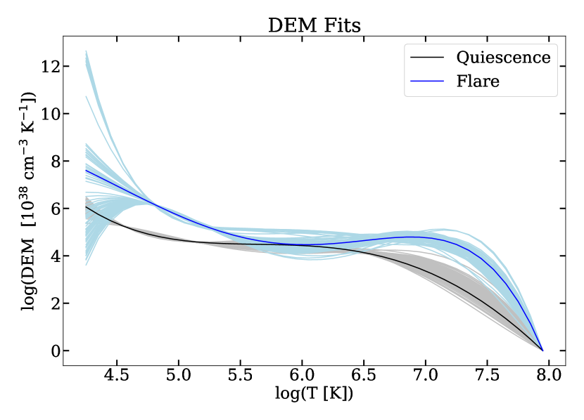
Figure 8: DEM distribution of Proxima Centauri for quiescent (black) and flaring (blue) periods with computed errors.

Moreover, we compare the line fluxes computed from this best-fit DEM function to the originally measured line fluxes. In Fig. 9 the ratios of measured to calculated fluxes of each emission line are plotted during quiescence (top panel) and flaring (bottom panel) periods. Regarding quiescence, the DEM model predicts the line fluxes well, except for the lines at highest peak formation temperature, which also exhibit the largest line flux error. The typically larger errors of the X-ray predictions are caused by the lower data quality of the Chandra observations. For flaring periods, all emission lines are also predicted within an acceptable deviation. An extreme outlier is only C ii, which is the line with the lowest peak formation temperature, which may indicate that a larger order of the Chebyshev polynomial is still needed to reduce the rigidity for the flaring DEM even further. Because optical depth effects may begin to play a role here, we decided against increasing the order of the polynomial since this moreover decreases the stability of the DEM fitting process. Furthermore, during the flaring state, all Fe lines are overpredicted, which may hint at an overestimated abundancy during flare or a slightly overpredicted DEM at these temperatures, since all Fe lines are clustered in temperature. Overall, the DEM is expected to yield better predictions for quiescence since the longer quiescent time spans allow one to accumulate more data than the shorter, though more intense, flaring periods. Finally, to get an idea about how well the DEM functions reflect the FUV and X-ray measurements and therefore the coronal (and transition region) temperature structure of Proxima Centauri, the flux ratio plot in Fig. 10 is complemented with the ratio of the DEM functions (red line). The DEM structure represents the flux ratio quite well, again with the exception of the very cool C ii. Since we do not have measurements of lines with a peak formation temperature between $\log$ T= 5.5-6.0, we cannot exclude that there is a rise to higher flare to quiescent ratios in this regime. Nevertheless, both X-ray and FUV data show a decrease of this ratio towards this temperature regime, making a trough-like structure, as depicted in Fig. 10, the most simple solution.

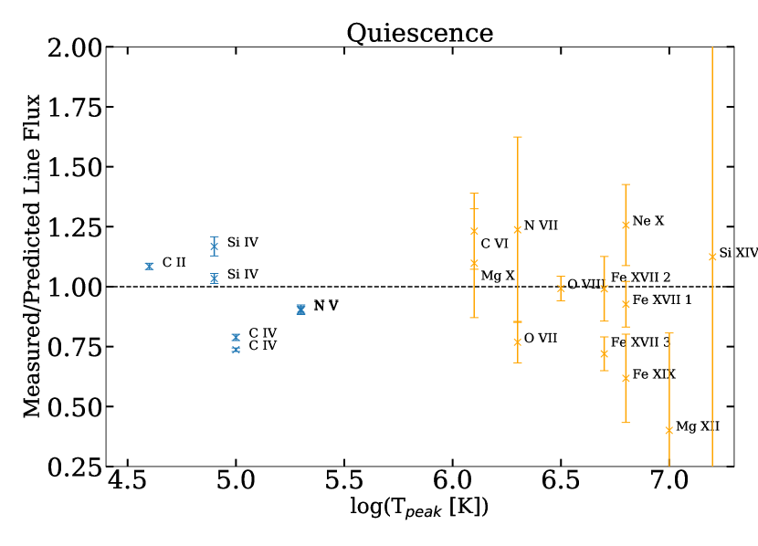
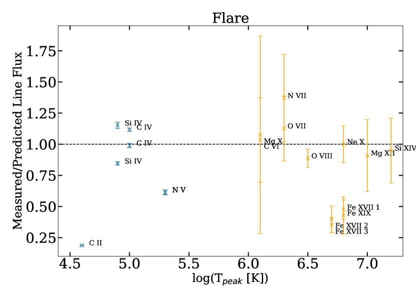
Figure 9: Flux ratios of measured to predicted quiescence line fluxes plotted against peak formation temperatures for quiescence (top) and flaring (bottom). The predicted fluxes were calculated with respective contribution functions and the determined DEM(T) distribution.

Figure 10: Flare to quiescence line flux ratios at their respective peak formation temperatures. The dashed black line indicates 1:1 ratios. An increase in the ratio is seen to lower and higher temperatures, respectively, with an exception for C II. The ratio of the flare and quiescence DEM(T) functions (red line) reproduces this behaviour roughly.

6.3 Synthetic spectra

From the DEM of the quiescent and flaring state, we calculated synthetic spectra in the range of 1 to 1700 Å , respectively, using a resolution of 1 Å. We show the synthetic spectra in Fig. 11 with a wavelength binning defined by a minimum flux density of $2\cdot 10^{-14}$ erg s^-1 cm^-2 Å^-1 per bin. Additionally, we show the flux density with a binning of 100 Å  and at a distance of 1 AU to Proxima Centauri for a better comparison to the synthetic spectra constructed recently by Duvvuri et al. (2021) for four M dwarfs. Of these, we indicate the flux density covered by GJ 832 and Trappist-1 in Fig.11. Our quiescent synthetic spectrum of Proxima Centauri shows a decline in the flux density in resemblance of their synthetic spectra of GJ 832 (M2/3) and Trappist-1 (M7.5), although the slope of our spectrum is somewhat flatter than for their spectra. Moreover, their synthetic spectrum of Barnard’s star (M4) during quiescence exhibits a slight increase in the flux density towards longer wavelengths, while being relatively constant at a wavelength below 800 Å. We find the slope of Proxima Centauri between those found for Barnard’s star and GJ 832, but with flux density values of Proxima Centauri more closely resembling those of GJ 832. This better agreement with an earlier spectral type may be explained by the higher activity level of Proxima Centauri compared to GJ 832, while Trappist-1 is again much less active than Proxima Centauri. Indeed, the flaring spectrum of Barnard’s star also constructed by Duvvuri et al. (2021) is again in close resemblance to our flaring spectrum.

Further, we compared our synthetic spectrum to those constructed by Loyd et al. (2016). We cannot reproduce the sharp drop at about 400 Å  seen in all of their mid M dwarf spectra, and we note that this feature is also absent in the spectra constructed by Duvvuri et al. (2021). Yet this feature is again seen in the composite spectrum of Proxima Centauri reported by Ribas et al. (2017), who used a variety of observations obtained with different instruments. Otherwise our quiescent synthetic spectrum is also in agreement with these observations.

Our synthetic spectra can further be used for an evaluation of the stability of the atmospheres of the two close-in planets in the system Proxima Centauri b and d (Faria et al. 2022) as was demonstrated for Barnard’s star by France et al. (2020). Since the mass loss is directly proportional to the flux in the XUV range and our flare spectrum shows a factor of about 5 higher for the integrated flux than the quiescent spectrum, even for our rather small flares, the expected mass loss is also sensitively dependent on the flare duty cycle of the star.

For a crude estimate of the mass loss, we followed the example of Owen & Jackson (2012) and Poppenhaeger et al. (2021), who employed the widely used equation for energy limited hydrodynamic escape $\dot{M}=\epsilon\frac{3\beta^{2}F_{XUV}}{4GK\rho_{pl}}$, with $\epsilon$ being the efficiency of atmospheric loss, which we estimate to be 0.1, with $K$ representing the impact of Roche overflow, which we estimate to be 1 (i.e. no Roche overflow). Furthermore, we estimate the ratio between the planetary radius and planetary FUV radius $\beta$ to be 1.5, since Proxima Centauri b and d are small planets. Finally, we estimate the planetary density $\rho_{pl}$ to be 5.0 g/cm³, which is slightly lower than the Earth’s density. From our synthetic spectra, we derived an integrated $F_{XUV}$ flux of 1.8 erg/s/cm² during quiescent intervals at the distance of Proxima Centauri b, and of 10.5 erg/s/cm² during flaring states, thus we estimate a present day mass loss of 0.4$\cdot 10^{9}$ g s^-1 during the quiescent and 2.1$\cdot 10^{9}$ g s^-1 during flaring state, respectively. Nevertheless, the detailed modelling of thermal and possibly non-thermal atmospheric escape induced by our synthetic spectra on the two close-in planets is beyond the scope of this paper.

Figure 11: Synthetic spectra in the range of 1 to 1700 Å, calculated from the DEMs for quiescent (black) and flaring (red) state of Proxima Centauri. The pink shaded region marks the wavelength coverage of our Chandra data, while the blue shaded region marks the coverage of the Hubble data. For the flaring state, the highest amplitude by far is seen for the Ly$\alpha$ line, which cannot be predicted well by our data since the line is formed at lower temperatures. The flux density was binned by a minimum flux of $2\cdot 10^{-14}$ erg s^-1 cm^-2 Å^-1 per bin (top) and by 100 Å  bins (bottom) at a distance of 1 AU.

7 Conclusion

In this work X-ray observations of Proxima Centauri taken by Chandra and simultaneous FUV spectra from Hubble/STIS were analysed. First, light curves were extracted, flaring as well as quiescent periods were determined, and associated spectra were generated. The spectra were used to measure 25 X-ray and 16 FUV emission lines out of which 12 and six, respectively, could be measured with a high enough precision for a DEM construction. Flare to quiescence flux ratios range from about 1 for example for Mg X up to 20 for Si IV. The observed line fluxes were used to construct the DEM of the optically thin coronal and transition region plasma. The DEM functions yield the strongest increases at temperatures $\log$T=4.25-5.5 (20 000-300 000 K, FUV regime) and beyond $\log$T=6.5 (3.1 MK, X-ray regime) during flares. Furthermore, flare and quiescent line fluxes were predicted with the help of the DEM curves and compared to measured values. For all but one very cool C ii line, the model predicts acceptable values. The same methods as used in this work can be applied to many other spectra, in particular to archival Proxima Centauri data. The DEM method does not strictly require simultaneous X-ray and UV observations, but it can be applied to X-ray and UV data individually, though each wavelength regime only would trace a certain range in plasma temperature. When using all suitable X-ray and UV observations, that is observations with sufficient spectral resolution and signal-to-noise, one can determine how the spectral shape varies with time (or activity level) and construct the irradiation spectrum of Proxima Centauri b for large ranges of conditions. These spectra can then be used to create sophisticated planetary atmosphere models, which will provide information about the conditions on Proxima Centauri b.

Appendix A Line lists

Here we state the measured line properties of X-ray and FUV lines in Tables 4 and 5.

Table 4: X-ray emission lines

Ion	Wavelength [$\mathring{A}$]	Net Line Flux [erg/s/cm2]	Net Line Counts	Background Counts	log(T${}_{\text{peak}}$ [K])
Quiescence
Si XIV	6.186	9.25$\cdot 10^{-15}\pm$ 1.45$\cdot 10^{-14}$	9.6 $\pm$ 15.1	109.33 $\pm$ 10.5	7.2
Mg XII	8.419	1.14$\cdot 10^{-14}\pm$ 1.15$\cdot 10^{-14}$	14.2 $\pm$ 14.4	97.3 $\pm$ 9.9	7.0
Ne X	12.138	1.03$\cdot 10^{-13}\pm$ 1.38$\cdot 10^{-14}$	137.7 $\pm$ 18.5	102.3 $\pm$ 10.1	6.8
Fe XVII	15.013	1.21$\cdot 10^{-13}\pm$ 1.24$\cdot 10^{-14}$	206.8 $\pm$ 21.2	121.6 $\pm$ 11.0	6.8
Fe XIX	15.208	3.37$\cdot 10^{-14}\pm$ 1.00$\cdot 10^{-14}$	58.3 $\pm$ 17.4	121.7 $\pm$ 11.0	6.8
Fe XVII	16.775	6.92$\cdot 10^{-14}\pm$ 9.42$\cdot 10^{-15}$	132.0 $\pm$ 18.0	95.3 $\pm$ 9.8	6.7
Fe XVII	17.096	1.23$\cdot 10^{-13}\pm$ 1.21$\cdot 10^{-14}$	202.6 $\pm$ 19.8	95.3 $\pm$ 9.8	6.7
O VIII	18.967	2.73$\cdot 10^{-13}\pm$ 1.41$\cdot 10^{-14}$	519.7 $\pm$ 26.8	100.3 $\pm$ 10.0	6.5
O VII	21.602	1.26$\cdot 10^{-13}\pm$ 1.42$\cdot 10^{-14}$	176.6 $\pm$ 19.9	109.6 $\pm$ 10.5	6.3
N VII	24.779	3.42$\cdot 10^{-14}\pm$ 1.07$\cdot 10^{-14}$	52.8 $\pm$ 16.47	109.3 $\pm$ 10.5	6.3
C VI	33.734	8.89$\cdot 10^{-14}\pm$ 1.14$\cdot 10^{-14}$	140.7 $\pm$ 18.1	94.0 $\pm$ 9.7	6.1
Mg X	57.876	2.04$\cdot 10^{-14}\pm$ 4.22$\cdot 10^{-15}$	70.4 $\pm$ 14.6	70.6 $\pm$ 8.4	6.1
Flare
Si XIV	6.186	3.40$\cdot 10^{-13}\pm$ 9.33$\cdot 10^{-14}$	27.1 $\pm$ 7.4	14.0$\pm$ 3.7	7.2
Mg XII	8.419	2.78$\cdot 10^{-13}\pm$ 8.82$\cdot 10^{-14}$	26.4 $\pm$ 8.4	22.0 $\pm$ 4.7	7.0
Ne X	12.138	8.05$\cdot 10^{-13}\pm$ 1.18$\cdot 10^{-13}$	82.4 $\pm$ 12.1	32.3 $\pm$ 5.7	6.8
Fe XVII	15.013	5.06$\cdot 10^{-13}\pm$ 8.31$\cdot 10^{-14}$	65.9 $\pm$ 10.8	25.6$\pm$5.1	6.8
Fe XIX	15.208	1.87$\cdot 10^{-13}\pm$ 6.58$\cdot 10^{-14}$	24.8 $\pm$ 8.7	25.6 $\pm$ 5.1	6.8
Fe XVII	16.775	2.02$\cdot 10^{-13}\pm$ 5.51$\cdot 10^{-14}$	29.7 $\pm$ 8.1	17.6$\pm$4.2	6.7
Fe XVII	17.096	4.29$\cdot 10^{-13}\pm$ 7.52$\cdot 10^{-14}$	53.9 $\pm$ 9.4	17.6$\pm$4.2	6.7
O VIII	18.967	1.15$\cdot 10^{-12}\pm$ 9.69$\cdot 10^{-14}$	167.1 $\pm$ 14.0	15.0$\pm$3.9	6.5
O VII	21.602	3.33$\cdot 10^{-13}\pm$ 7.69$\cdot 10^{-14}$	35.6 $\pm$ 8.2	16.0$\pm$4.0	6.3
N VII	24.779	2.27 $\cdot 10^{-13}\pm$ 5.79$\cdot 10^{-14}$	26.8 $\pm$ 6.8	10.0 $\pm$ 3.1	6.3
C VI	33.734	1.51$\cdot 10^{-13}\pm$ 4.98$\cdot 10^{-14}$	18.4 $\pm$ 6.0	9.0$\pm$3.0	6.1
Mg X	57.876	2.26$\cdot 10^{-14}\pm$ 1.66$\cdot 10^{-14}$	6.0 $\pm$ 4.4	6.6$\pm$2.6	6.1

Table 5: FUV emission lines

Ion	Wavelength [$\mathring{A}$]	Net Line Flux [erg/s/cm2]	Net Line Counts	Red-shift [km/s]	log(T${}_{\text{peak}}$ [K])
Quiescence
N V	1238.823	5.60$\cdot 10^{-14}\pm 1.03\cdot 10^{-15}$	2782.7 $\pm$ 51.1	-22.8	5.3
N V	1242.806	2.81$\cdot 10^{-14}\pm 5.52\cdot 10^{-16}$	2339.7 $\pm$ 47.2	-21.6	5.3
C II	1335.710	5.36$\cdot 10^{-14}\pm 6.42\cdot 10^{-16}$	6292.7 $\pm$ 72.7	-23.2	4.6
Si IV	1393.757	2.35$\cdot 10^{-14}\pm 4.76\cdot 10^{-16}$	2573.7 $\pm$ 48.5	-20.6	4.9
Si IV	1402.772	1.33$\cdot 10^{-14}\pm 4.56\cdot 10^{-16}$	928.6 $\pm$ 32.5	-21.2	5.0
C IV	1548.189	1.54$\cdot 10^{-13}\pm 1.55\cdot 10^{-15}$	8187.6 $\pm$ 84.7	-18.7	5.0
C IV	1550.775	8.25$\cdot 10^{-14}\pm 1.38\cdot 10^{-15}$	3623.5 $\pm$ 62.0	-22.2	4.9
Flare
N V	1238.823	2.28$\cdot 10^{-13}\pm 6.62\cdot 10^{-15}$	1072.5 $\pm$ 30.4	-22.7	5.3
N V	1242.806	1.13$\cdot 10^{-13}\pm 3.63\cdot 10^{-15}$	893.1 $\pm$ 27.3	-21.1	5.3
C II	1335.710	2.46$\cdot 10^{-13}\pm 4.75\cdot 10^{-15}$	2731.7 $\pm$ 55.7	-21.6	4.6
Si IV	1393.757	3.86$\cdot 10^{-13}\pm 5.79\cdot 10^{-15}$	3987.3 $\pm$ 60.2	-20.4	4.9
Si IV	1402.772	2.63$\cdot 10^{-13}\pm 6.00\cdot 10^{-15}$	1726.1 $\pm$ 41.5	-20.4	5.0
C IV	1548.189	1.73$\cdot 10^{-12}\pm 2.16\cdot 10^{-14}$	7444.6 $\pm$ 102.4	-17.4	5.0
C IV	1550.775	7.69$\cdot 10^{-13}\pm 1.38\cdot 10^{-14}$	3184.8 $\pm$ 54.1	-22.0	4.9

References

- Anders & Grevesse (1989) Anders, E. & Grevesse, N. 1989, Geochim. Cosmochim. Acta., 53, 197
- Anglada-Escudé et al. (2016) Anglada-Escudé, G., Amado, P. J., Barnes, J., et al. 2016, Nature, 536, 437
- Audard et al. (2003) Audard, M., Güdel, M., Sres, A., Raassen, A. J. J., & Mewe, R. 2003, A&A, 398, 1137
- Benedict et al. (1998) Benedict, G. F., McArthur, B., Nelan, E., et al. 1998, AJ, 116, 429
- Benz (2017) Benz, A. O. 2017, Living Reviews in Solar Physics, 14, 2
- Bessell (1991) Bessell, M. 1991, 101
- Craig & Brown (1976) Craig, I. J. D. & Brown, J. C. 1976, Astronomy and Astrophysics, 49, 239
- Doyle & Butler (1990) Doyle, J. & Butler, C. 1990, Astronomy and astrophysics (Berlin. Print), 235, 335
- Duvvuri et al. (2021) Duvvuri, G. M., Sebastian Pineda, J., Berta-Thompson, Z. K., et al. 2021, ApJ, 913, 40
- Faria et al. (2022) Faria, J. P., Suárez Mascareño, A., Figueira, P., et al. 2022, A&A, 658, A115
- France et al. (2020) France, K., Duvvuri, G., Egan, H., et al. 2020, AJ, 160, 237
- Fuhrmeister et al. (2011) Fuhrmeister, B., Lalitha, S., Poppenhaeger, K., et al. 2011, Astronomy and Astrophysics, 534, 1
- Gaia Collaboration (2018) Gaia Collaboration. 2018, VizieR Online Data Catalog, I/345
- García Muñoz (2007) García Muñoz, A. 2007, Planet. Space Sci., 55, 1426
- Grevesse & Sauval (1999) Grevesse, N. & Sauval, A. J. 1999, A&A, 347, 348
- Güdel (2004) Güdel, M. 2004, Astronomy and Astrophysics Review, 12
- Güdel et al. (2004) Güdel, M., Audard, M., Reale, F., Skinner, S. L., & Linsky, J. L. 2004, Astronomy & Astrophysics, 416, 713
- Haisch et al. (1990) Haisch, B. M., Butler, C. J., Foing, B., Rodono, M., & Giampapa, M. S. 1990, Astronomy and Astrophysics, 232, 387
- Haisch et al. (1980) Haisch, B. M., Harnden, F. R., J., Seward, F. D., et al. 1980, ApJ, 242, L99
- Howard et al. (2020) Howard, W. S., Corbett, H., Law, N. M., et al. 2020, ApJ, 902, 115
- Howard et al. (2018) Howard, W. S., Tilley, M. A., Corbett, H., et al. 2018, The Astrophysical Journal, 860, L30
- Klein et al. (2021) Klein, B., Donati, J.-F., Hébrard, É. M., et al. 2021, MNRAS, 500, 1844
- Koskinen et al. (2010) Koskinen, T. T., Cho, J. Y., Achilleos, N., & Aylward, A. D. 2010, Astrophysical Journal, 722, 178
- Lalitha et al. (2020) Lalitha, S., Schmitt, J. H. M. M., Singh, K. P., et al. 2020, MNRAS, 498, 3658
- Landi & Chiuderi Drago (2008) Landi, E. & Chiuderi Drago, F. 2008, The Astrophysical Journal, 675, 1629
- Liefke et al. (2008) Liefke, C., Ness, J. U., Schmitt, J. H. M. M., & Maggio, A. 2008, A&A, 491, 859
- Loyd et al. (2016) Loyd, R. O. P., France, K., Youngblood, A., et al. 2016, ApJ, 824, 102
- Loyd et al. (2018) Loyd, R. O. P., France, K., Youngblood, A., et al. 2018, The Astrophysical Journal, 867, 71
- Luger & Barnes (2015) Luger, R. & Barnes, R. 2015, Astrobiology, 15, 119
- MacGregor et al. (2021) MacGregor, M. A., Weinberger, A. J., Loyd, R. O. P., et al. 2021, ApJ, 911, L25
- Murray-Clay et al. (2009) Murray-Clay, R. A., Chiang, E. I., & Murray, N. 2009, Astrophysical Journal, 693, 23
- Ness et al. (2002) Ness, J. U., Schmitt, J. H. M. M., Burwitz, V., et al. 2002, A&A, 394, 911
- Owen & Jackson (2012) Owen, J. E. & Jackson, A. P. 2012, MNRAS, 425, 2931
- Poppenhaeger et al. (2021) Poppenhaeger, K., Ketzer, L., & Mallonn, M. 2021, MNRAS, 500, 4560
- Reiners (2012) Reiners, A. 2012, Living Reviews in Solar Physics, 9, 1
- Reiners & Basri (2008) Reiners, A. & Basri, G. 2008, A&A, 489, L45
- Ribas et al. (2017) Ribas, I., Gregg, M. D., Boyajian, T. S., & Bolmont, E. 2017, A&A, 603, A58
- Robrade & Schmitt (2005) Robrade, J. & Schmitt, J. H. M. M. 2005, A&A, 435, 1073
- Salz et al. (2016) Salz, M., Czesla, S., Schneider, P. C., & Schmitt, J. H. M. M. 2016, A&A, 586, A75
- Schmitt & Ness (2004) Schmitt, J. H. & Ness, J. U. 2004, Astronomy and Astrophysics, 415, 1099
- Ségransan et al. (2003) Ségransan, D., Kervella, P., Forveille, T., & Queloz, D. 2003, Astronomy and Astrophysics, 397 [arXiv:0211647]
- Smith et al. (2001) Smith, R. K., Brickhouse, N. S., Liedahl, D. A., & Raymond, J. C. 2001, ApJ, 556, L91
- Tilley et al. (2019) Tilley, M. A., Segura, A., Meadows, V., Hawley, S., & Davenport, J. 2019, Astrobiology, 19, 64
- Ward-Duong et al. (2021) Ward-Duong, K., Branton, D., Carlberg, J., et al. 2021, in American Astronomical Society Meeting Abstracts, Vol. 53, American Astronomical Society Meeting Abstracts, 350.04
- Weisskopf et al. (2002) Weisskopf, M. C., Brinkman, B., Canizares, C., et al. 2002, PASP, 114, 1