An intersecting problem of graph-directed
attractors and an application

Abstract.

Let $(K_{1},\ldots,K_{n})$ be a Cantor type graph-directed attractors in $\mathbb{R}^{d}$. By creating an auxiliary graph, we provide an effective criterion of whether $K_{i}\cap K_{j}$ is empty for every pair of $1\leq i,j\leq n$. Moreover, the emptiness can be checked by examining only a finite number of the attractor’s geometric approximations. The method is also applicable for more general graph-directed systems. As an application, we are able to determine the connectedness of all $d$-dimensional generalized Sierpiński sponges of which the corresponding IFSs are allowed to have rotational and reflectional components.

1. Introduction

Graph-directed sets constitute a frequently explored class of typical fractals. These sets can be regarded as a generalization of self-similar sets, and the standard process of generating them is as follows. Let $G=G(\mathcal{V},\mathcal{E})$ be a directed graph where $\mathcal{V}=\{1,2,\ldots,n\}$ is the vertex set and $\mathcal{E}$ is the edge set. Assume further that for each vertex in $\mathcal{V}$, there is at least one edge starting from it. A graph-directed IFS (iterated function system) in $\mathbb{R}^{d}$ is a finite family $\Phi=\{\varphi_{e}:e\in\mathcal{E}\}$ consisting of contracting similarities from $\mathbb{R}^{d}$ to $\mathbb{R}^{d}$ indexed by edges in $\mathcal{E}$. It is well known (please see [9] or [20]) that there is a unique $n$-tuple of non-empty compact sets $(K_{1},\ldots,K_{n})$ such that

$$K_{i}=\bigcup_{j=1}^{n}\bigcup_{e\in\mathcal{E}_{i,j}}\varphi_{e}(K_{j}),$$

where $\mathcal{E}_{i,j}$ denotes the collection of edges in $\mathcal{E}$ from $i$ to $j$. Such a tuple is usually called the graph-directed attractor associated with the graph-directed system $(G,\Phi)$, and the corresponding graph-directed set often refers to the union $\bigcup_{i=1}^{n}K_{i}$.

In [20], Mauldin and Williams calculated the Hausdorff dimension of graph-directed sets under an open set type condition. It is also demonstrated that the corresponding Hausdorff measure of the set is positive and $\sigma$-finite. Later, Das and Ngai [5] developed algorithms to compute the dimension under some weak separation condition (called the finite type condition). Xiong and Xi [31] investigated the Lipschitz classification of dust-like graph-directed sets. For further work, please refer to [7, 8, 11, 21, 22, 29, 30] and references therein. Results on graph-directed sets can also shed some light on the study of self-similar or self-affine sets with overlaps. We refer the interested readers to [14, 16, 18, 24].

We may always assume safely that for $1\leq i\leq n$, $\varphi_{e}\neq\varphi_{e^{\prime}}$ whenever $e,e^{\prime}\in\mathcal{E}_{i,j}$ are distinct. We also remark that for every vertex $v$ of every graph appeared in this paper, one is able to travel from $v$ directly to itself if and only if there is a loop at $v$.

Let $(K_{1},\ldots,K_{n})$ be a graph-directed attractor. Apart from the fractal dimensions of $\bigcup_{i=1}^{n}K_{i}$, the relationship between any pair of sets in that tuple is also worthy of attention. For example, given distinct $1\leq i,j\leq n$, it is interesting to ask whether $K_{i}$ intersects $K_{j}$, especially when $K_{1},\ldots,K_{n}$ are all “spread” in one common area.

In this paper, we solve this intersecting problem for a special class of graph-directed sets and apply the solution to a connectedness problem of the so-called sponge-like sets (which will be introduced later). Although our approach remains valid under a more general setting (please see Section 4 for details), the treatment on the following class, namely Cantor type graph-directed attractors, would be adequate to demonstrate the idea.

Definition 1.1.

Let $(K_{1},\ldots,K_{n})$ be a graph-directed attractor in $\mathbb{R}^{d}$ associated with $G=G(\mathcal{V},\mathcal{E})$ and $\Phi=\{\varphi_{e}:e\in\mathcal{E}\}$. We say that the attractor $(K_{1},\ldots,K_{n})$ or the IFS $\Phi$ is of Cantor type if for each $e\in\mathcal{E}$, $\varphi_{e}$ is a contracting similarity on $\mathbb{R}^{d}$ of the form $\varphi_{e}(x)=N^{-1}(x+t_{e})$, where $N\geq 2$ is an integer and $t_{e}\in\{0,1,\ldots,N-1\}^{d}$.

Let $(K_{1},\ldots,K_{n})$ be a Cantor type graph-directed attractor in $\mathbb{R}^{d}$. The following geometric iteration process to obtain the attractor is standard, and we present here a sketch of proof just for completeness.

Lemma 1.2.

Let $Q_{i,0}:=[0,1]^{d}$ for $1\leq i\leq n$ and recursively define

$$Q_{i,k}:=\bigcup_{j=1}^{n}\bigcup_{e\in\mathcal{E}_{i,j}}\varphi_{e}(Q_{j,k-1}),\quad k\geq 1,1\leq i\leq n.$$

Then for each $i$, $\{Q_{i,k}\}_{k=1}^{\infty}$ forms a decreasing sequence of compact sets and $K_{i}=\bigcap_{k=1}^{\infty}Q_{i,k}$.

We name $Q_{i,k}$ the level-$k$ approximation of $K_{i}$.

Proof.

It is easy to see that

$$\varphi_{e}(Q_{i,0})=\varphi_{e}([0,1]^{d})\subset[0,1]^{d}=Q_{i,0},\quad\forall e\in\mathcal{E},1\leq i\leq n,$$

from which one can show by induction that $\{Q_{i,k}\}_{k=1}^{\infty}$ is decreasing. Note that $Q_{i,k}$ is a finite union of closed cubes and hence is compact. Finally, it follows from

$$\bigcap_{k=1}^{\infty}Q_{i,k}=\bigcap_{k=1}^{\infty}\Big{(}\bigcup_{j=1}^{n}\bigcup_{e\in\mathcal{E}_{i,j}}\varphi_{e}(Q_{j,k-1})\Big{)}=\bigcup_{j=1}^{n}\bigcup_{e\in\mathcal{E}_{i,j}}\varphi_{e}\Big{(}\bigcap_{k=1}^{\infty}Q_{j,k-1}\Big{)}$$

and the uniqueness of the graph-directed attractor that $K_{i}=\bigcap_{k=1}^{\infty}Q_{i,k}$. ∎

For convenience and clarity, we will denote $\mathcal{V}_{n}:=\{1,\ldots,n\}$ throughout this paper. The desired solution of the aforementioned problem is attained with the aid of a readily created graph called the intersecting graph. Please see Definition 2.9 for its construction.

Our criterion is:

Theorem 1.3.

Let $(K_{1},\ldots,K_{n})$ be a Cantor type graph-directed attractor in $\mathbb{R}^{d}$. For every pair of distinct $i,j\in\mathcal{V}_{n}$, $K_{i}\cap K_{j}\neq\varnothing$ if and only if there exists, in the associated intersecting graph, either a terminated finite walk or an infinite solid walk that starts from $(i,j)$.

It is also worthwhile considering the intersecting problem from a different perspective: Is there a constant $C$ such that for every pair of $i\neq j$, $K_{i}\cap K_{j}\neq\varnothing$ whenever $Q_{i,C}\cap Q_{j,C}\neq\varnothing$? The answer is actually affirmative. Write

(1.1) $$c(n,d):=(d-1)n^{2}+\frac{n^{2}+n}{2}+d-1,\quad d\geq 1.$$

By analyzing walks in the associated intersecting graph, we have the following result.

Theorem 1.4.

Let $(K_{1},\ldots,K_{n})$ be a Cantor type graph-directed attractor in $\mathbb{R}^{d}$. Assume that $i,j\in\mathcal{V}_{n}$ are distinct. Then $K_{i}\cap K_{j}\neq\varnothing$ if and only if $Q_{i,c(n,d)}\cap Q_{j,c(n,d)}\neq\varnothing$.

Our results on the intersecting problem can be used to characterize the connectedness of some specific fractals. Note that connected fractals constitute an important class of fractals. Related results can be found in [4, 6, 26, 27, 28] and etc. But to tell whether a given fractal is connected or not is a nontrivial question. In a classical paper [15], Hata transformed the connectedness problem of attractors of IFSs elegantly into a connectedness problem of graphs.

Theorem 1.5 (Hata [15]).

Let $\Phi=\{\varphi_{i}\}_{i=1}^{n}$ be an IFS on $\mathbb{R}^{d}$ and let $K$ be its attractor. Then $K$ is connected if and only if the associated Hata graph is connected, where the Hata graph is defined as follows.

1. The vertex set is the index set $\{1,\ldots,n\}$;

2. There is an edge joining distinct $1\leq i,j\leq n$ if and only if $\varphi_{i}(K)\cap\varphi_{j}(K)\neq\varnothing$.

However, the examination of whether $\varphi_{i}(K)\cap\varphi_{j}(K)\neq\varnothing$ is a hard task in many circumstances, even when $K$ is self-similar. Since all the ingredients in hand is the IFS itself, we usually have to choose a suitable compact invariant set (with respect to the IFS), iterate it several times, and hope to obtain useful information on the connectedness of the limit set. We shall focus on “sponge-like” self-similar sets defined as follows. Denote $\mathcal{O}_{d}$ to be the group of symmetries of the $d$-cube $[0,1]^{d}$. That is to say, $\mathcal{O}_{d}$ consists of all isometries that maps $[0,1]^{d}$ onto itself. Let $N\geq 2$ be an integer and let $\mathcal{I}\subset\{0,1,\ldots,N-1\}^{d}$ be a non-empty set with $1<|\mathcal{I}|<N^{d}$, where $|\mathcal{I}|$ denotes the cardinality of $\mathcal{I}$. Suppose for each $i\in\mathcal{I}$ there corresponds a contracting map

$$\varphi_{i}(x)=\frac{1}{N}(O_{i}(x)+i),\quad x\in\mathbb{R}^{d},$$

where $O_{i}\in\mathcal{O}_{d}$. A classical result of Hutchinson [17] states that there is a unique non-empty compact set $F=F(d,N,\mathcal{I})$ such that $F=\bigcup_{i\in\mathcal{I}}\varphi_{i}(F)$. When $O_{i}=\operatorname{id}$ for all $i\in\mathcal{I}$, the attractor $F$ is usually called a Sierpiński sponge when $d\geq 3$ and a generalized Sierpiński carpet or a fractal square when $d=2$. For convenience, we shall name the attractor $F$ (under our setting) a sponge-like set throughout this paper. These sets can be obtained by the following geometric iteration process: Writing $F_{0}:=[0,1]^{d}$ and recursively defining $F_{k}:=\bigcup_{i\in\mathcal{I}}\varphi_{i}(F_{k-1})$ for $k\geq 1$, then $F=\bigcap_{k=0}^{\infty}F_{k}$. It is easy to observe that $F_{k}$ is a finite union of closed cubes of side length $N^{-k}$.

Example 1.6.

Let $d=2$, $N=2$ and let $\mathcal{I}=\{(0,0),(1,0),(0,1)\}$. In Figure 1, we show attractors associated with the following three IFSs from left to right:

1. $O_{i}\equiv\operatorname{id}$ for $i\in\mathcal{I}$;

2. $O_{(0,0)}=\operatorname{id}$, while $O_{(0,1)},O_{(1,0)}$ are rotations of $90^{\circ}$ and $270^{\circ}$ (counterclockwise), respectively;

3. $O_{(0,1)}$ is the rotation of $90^{\circ}$ (counterclockwise), while $O_{(0,0)},O_{(1,0)}$ are flips along the lines $x=\frac{1}{2}$ and $y=\frac{1}{2}$, respectively.

Interested readers can find an illustration of all possible attractors in the case when $d=2$, $N=2$ and $|\mathcal{I}|=3$ in the book [23, Section 5.3].

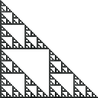
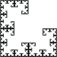
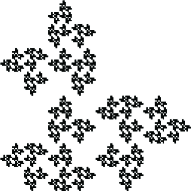
Figure 1. Three sponge-like sets in $\mathbb{R}^{2}$

Over the last decade, sponge-like sets have been studied intensely, especially cases when all of the contracting maps in the IFS are orientation preserving. Unfortunately, even for this specific class of self-similar sets, many basic topological properties are still far from clear to us. Criteria for generalized Sierpiński carpets that are totally disconnected or have only finitely many connected components are given in [19] and [33], respectively. Partial results on the quasisymmetric and Lipschitz classification of Sierpiński sponges can be found in [2, 3, 25, 32] and references therein. In a recent paper [4] joint with Dai, Luo and Wang, the authors provided characterizations of connected Sierpiński carpets with local cut points.

For general cases allowing rotations and reflections, the topology becomes involved and there are rare existing studies. For example, it is simple to observe that there are $|\mathcal{O}_{d}|^{|\mathcal{I}|}$ different IFSs provided $\mathcal{I}$ is fixed, but the enumeration of distinct attractors is difficult since many of them coincide. This problem was solved in [10] by Falconer and O’Conner using group theory. In the case when $d=2$, Fraser [12] investigated the self-affine generalization of our sponge-like sets and calculated their packing and box dimensions under some open set type condition.

With the aid of Theorem 1.3, we are able to draw the Hata graph associated with any given sponge-like set and hence to determine whether it is connected. Please see Section 3 for details. As a corollary of Theorem 1.4, we also show that it suffices to check only a finite number of its geometric approximations.

Theorem 1.7.

Let $F=F(d,N,\mathcal{I})$ be a sponge-like set in $\mathbb{R}^{d}$. Then $F$ is connected if and only if $F_{C(d)+1}$ is connected, where $C(d):=c(d!2^{d}+2,d)-1$ and $c(\cdot,\cdot)$ is as in (1.1).

The paper is organized as follows. In Section 2, we construct the intersecting graph and prove Theorem 1.3. In Section 3, we prove Theorem 1.4 and discuss the sharpness of the constant $c(n,d)$. In Section 4, we present the method of plotting Hata graphs associated with sponge-like sets and prove Theorem 1.7. Section 3.2 is devoted to discussions on possible improvements of the constant $C(d)$ in Theorem 1.7 under suitable conditions. Finally, we discuss general settings under which our approach remains applicable in the last section.

2. The intersecting problem I: Creating auxiliary graphs

Throughout this section, $(K_{1},\ldots,K_{n})$ is presumed to be a fixed graph-directed attractor in $\mathbb{R}^{d}$ which is of Cantor type, and the notations $G=G(\mathcal{V}_{n},\mathcal{E})$, $\mathcal{E}_{i,j}$, $\varphi_{e}$, $t_{e}$, $Q_{i,k}$, etc. are as in Section 1. Here is a concrete example.

Example 2.1.

Let $G$ be the directed graph as in Figure 2. Set $d=1$, $N=4$ and

$$\varphi_{e_{1}}(x)=\varphi_{e_{3}}(x)=\frac{x}{4},\,\varphi_{e_{2}}(x)=\frac{x}{4}+\frac{1}{4},\,\varphi_{e_{4}}(x)=\frac{x}{4}+\frac{3}{4}.$$

So $t_{e_{1}}=t_{e_{3}}=0$, $t_{e_{2}}=1$ and $t_{e_{4}}=3$. Clearly, $\{\varphi_{e_{i}}:1\leq i\leq 4\}$ is of Cantor type.

Figure 2.

For $k\geq 1$ and $i\in\mathcal{V}_{n}$, denote $\mathcal{E}_{i}^{k}$ to be the collection of walks in the directed graph $G$ which starts from $i$ and has length $k$. For $\mathbf{e}=(e_{1},\ldots,e_{k})\in\mathcal{E}_{i}^{k}$, denote by $\operatorname{ter}(\mathbf{e})$ the terminal vertex of $\mathbf{e}$ and write $\varphi_{\mathbf{e}}:=\varphi_{e_{1}}\circ\cdots\circ\varphi_{e_{k}}$.

Lemma 2.2.

Let $k\geq 1$ and let $i\in\mathcal{V}_{n}$. Then for each $t\geq 0$,

$$Q_{i,k+t}=\bigcup_{\mathbf{e}\in\mathcal{E}_{i}^{k}}\varphi_{\mathbf{e}}(Q_{\operatorname{ter}(\mathbf{e}),t}).$$

As a result, $K_{i}=\bigcup_{\mathbf{e}\in\mathcal{E}_{i}^{k}}\varphi_{\mathbf{e}}(K_{\operatorname{ter}(\mathbf{e})})$.

Proof.

The proof is straightforward: Just note that

$$Q_{i,k+t} =\bigcup_{j_{1}=1}^{n}\bigcup_{e_{1}\in\mathcal{E}_{i,j_{1}}}\varphi_{e_{1}}(Q_{j_{1},k+t-1})$$

$$=\bigcup_{j_{1}=1}^{n}\bigcup_{e_{1}\in\mathcal{E}_{i,j_{1}}}\varphi_{e_{1}}\Big{(}\bigcup_{j_{2}=1}^{n}\bigcup_{e_{2}\in\mathcal{E}_{j_{1},j_{2}}}\varphi_{e_{2}}(Q_{j_{2},k+t-2})\Big{)}$$

$$=\cdots=\bigcup_{\mathbf{e}\in\mathcal{E}_{i}^{k}}\varphi_{\mathbf{e}}(Q_{\operatorname{ter}(\mathbf{e}),t}).$$

As a result,

$$K_{i}=\bigcap_{t=0}^{\infty}Q_{i,k+t}=\bigcap_{t=0}^{\infty}\bigcup_{\mathbf{e}\in\mathcal{E}_{i}^{k}}\varphi_{\mathbf{e}}(Q_{\operatorname{ter}(\mathbf{e}),t})=\bigcup_{\mathbf{e}\in\mathcal{E}_{i}^{k}}\varphi_{\mathbf{e}}\Big{(}\bigcap_{t=0}^{\infty}Q_{\operatorname{ter}(\mathbf{e}),t}\Big{)}=\bigcup_{\mathbf{e}\in\mathcal{E}_{i}^{k}}\varphi_{\mathbf{e}}(K_{\operatorname{ter}(\mathbf{e})}).$$

∎

In particular, $Q_{i,k}=\bigcup_{\mathbf{e}\in\mathcal{E}_{i}^{k}}\varphi_{\mathbf{e}}([0,1]^{d})$. For narrative convenience, we shall call any cube in $\bigcup_{i=1}^{n}\{\varphi_{\mathbf{e}}([0,1]^{d}):\mathbf{e}\in\mathcal{E}_{i}^{k}\}$ a level-$k$ cube. Note that every $Q_{i,k}$ is the union of finite number of level-$k$ cubes.

Recall that for any given polytope $P\subset\mathbb{R}^{d}$, a face of $P$ is any set (including the empty set) of the form $P\cap\{x\in\mathbb{R}^{d}:ax=b\}$, where $a\in\mathbb{R}^{d}$, $b\in\mathbb{R}$ and the inequality $ax\leq b$ is valid for all $x\in P$ (please see [34]). Moreover, the dimension of a face is just the dimension of its affine hull. For example, faces of the unit cube $[0,1]^{d}$ of dimensions $0$ and $1$ are vertices and edges of $[0,1]^{d}$, respectively. Since the graph-directed attractor is of Cantor type, it is not hard to see that every level-$k$ cube can be written as

$$\Big{[}\frac{p_{1}}{N^{k}},\frac{p_{1}+1}{N^{k}}\Big{]}\times\Big{[}\frac{p_{2}}{N^{k}},\frac{p_{2}+1}{N^{k}}\Big{]}\times\cdots\times\Big{[}\frac{p_{d}}{N^{k}},\frac{p_{d}+1}{N^{k}}\Big{]}$$

for some integers $0\leq p_{1},\ldots,p_{d}\leq N^{k}-1$. Consequently, the intersection of any pair of level-$k$ cubes is just the largest common face they share.

2.1. Examination of faces of the unit cube

Let us address a preliminary question before moving on to the intersecting problem: Given any face $P$ of $[0,1]^{d}$ with $0\leq\dim P\leq d-1$, which of $K_{1},\ldots,K_{n}$ intersect it? We first record a simple observation.

Lemma 2.3.

Let $P$ be a face of $[0,1]^{d}$ with $0\leq\dim P\leq d$ and let $\varphi(x)=N^{-1}(x+t)$ where $t=(t_{1},\ldots,t_{d})\in\{0,1,\ldots,N-1\}^{d}$. We have for all $E\subset[0,1]^{d}$ that $P\cap\varphi(E)\subset\varphi(E\cap P)$. Furthermore, if $P\cap\varphi(E)$ is non-empty then it equals $\varphi(P\cap E)$.

Proof.

If $\dim P=d$ then $P$ is the unit cube itself and there is nothing to prove. So it suffices to consider cases when $\dim P\leq d-1$. Letting $s:=d-\dim P$, we can find a $0$-$1$ vector $\alpha=(a_{1},\ldots,a_{s})$ and a sequence $1\leq m_{1}<m_{2}<\cdots<m_{s}\leq d$ such that

(2.1) $$P=\{(x_{1},\ldots,x_{d})\in[0,1]^{d}:x_{m_{k}}=a_{k},1\leq k\leq s\}.$$

If $P\cap\varphi(E)=\varnothing$ then the inclusion clearly holds, so we may assume that $P\cap\varphi(E)\neq\varnothing$. Choosing any $y\in P\cap\varphi(E)$, there is some $(x_{1},\ldots,x_{d})\in E$ such that $y=\varphi(x_{1},\ldots,x_{d})=N^{-1}(x_{1}+t_{1},\ldots,x_{d}+t_{d})$. Since $y\in P$, $N^{-1}(x_{m_{k}}+t_{m_{k}})=a_{k}$ for $1\leq k\leq s$. If $a_{k}=0$ then $x_{m_{k}}+t_{m_{k}}=0$. So $x_{m_{k}}=t_{m_{k}}=0=a_{k}$. If $a_{k}=1$ then $x_{m_{k}}+t_{m_{k}}=N$. Since $t_{m_{k}}\leq N-1$, we have $x_{m_{k}}=1=a_{k}$ and $t_{m_{k}}=N-1$. We conclude that $x_{m_{k}}=a_{k}$ for $1\leq k\leq s$ so $(x_{1},\ldots,x_{d})\in P$. Thus $y=\varphi(x_{1},\ldots,x_{d})\in\varphi(P\cap E)$. Since $y$ is arbitrarily chosen, $P\cap\varphi(E)\subset\varphi(P\cap E)$.

On the other hand, let $z=(z_{1},\ldots,z_{d})\in P\cap E$. It follows from the definition of $P$ that $z_{m_{k}}=a_{k}$ for $1\leq k\leq s$. Since $P\cap\varphi(E)\not=\varnothing$, from the above argument, $t_{m_{k}}=a_{k}$ if $a_{k}=0$ and $t_{m_{k}}=N-1$ if $a_{k}=1$. Thus $z_{m_{k}}+t_{m_{k}}=Na_{k}$ for $1\leq k\leq s$ so that

$$N^{-1}(z_{m_{k}}+t_{m_{k}})=a_{k}.$$

This implies that $\varphi(z)\in P$ and hence $\varphi(P\cap E)\subset P\cap\varphi(E)$. So $\varphi(P\cap E)=P\cap\varphi(E)$. ∎

Corollary 2.4.

Let $\alpha$ be a vertex of $[0,1]^{d}$ and let $e\in\mathcal{E}$. If $\alpha\in\varphi_{e}([0,1]^{d})$ then $\alpha=\varphi_{e}(\alpha)$. Moreover, $\varphi_{e}(x)\neq\alpha$ whenever $x\neq\alpha$.

Proof.

Since $\alpha$ is a $0$-dimensional face of $[0,1]^{d}$, Lemma 2.3 implies that

$$\{\alpha\}=\{\alpha\}\cap\varphi_{e}([0,1]^{d})=\{\varphi_{e}(\alpha)\}$$

and hence $\alpha=\varphi_{e}(\alpha)$. The second statement clearly holds since $\varphi_{e}$ is injective. ∎

The following corollary will be used later.

Corollary 2.5.

Let $\varphi_{1}(x)=N^{-1}(x+t_{1}),\ldots,\varphi_{m}(x)=N^{-1}(x+t_{m})$ be contracting similarities with $t_{1},\ldots,t_{m}\in\{0,1,\ldots,N-1\}^{d}$. Let $P$ be a face of $[0,1]^{d}$ with $1\leq\dim P\leq d$. If $\varphi_{i}([0,1]^{d})\cap P\neq\varnothing$ for all $1\leq i\leq m$ then

$$\big{(}\varphi_{1}\circ\cdots\circ\varphi_{m}([0,1]^{d})\big{)}\cap P=\big{(}\varphi_{1}\circ\cdots\circ\varphi_{m}(P)\big{)}\cap P.$$

Proof.

We will prove this by induction on $m$. When $m=1$, this is just Lemma 2.3. Suppose the result holds for $1\leq m\leq k$. Then

$$\big{(}\varphi_{1}\circ\cdots\circ\varphi_{k+1}([0,1]^{d})\big{)}\cap P =\big{(}\varphi_{1}\circ\cdots\circ\varphi_{k+1}([0,1]^{d})\big{)}\cap\big{(}\varphi_{1}\circ\cdots\circ\varphi_{k}([0,1]^{d})\big{)}\cap P$$

$$=\big{(}\varphi_{1}\circ\cdots\circ\varphi_{k+1}([0,1]^{d})\big{)}\cap\big{(}\varphi_{1}\circ\cdots\circ\varphi_{k}(P)\big{)}\cap P$$

$$=\big{(}\varphi_{1}\circ\cdots\circ\varphi_{k}(\varphi_{k+1}([0,1]^{d})\cap P)\big{)}\cap P$$

$$=\big{(}\varphi_{1}\circ\cdots\circ\varphi_{k}\circ\varphi_{k+1}(P)\big{)}\cap P,$$

as desired. ∎

Let $P$ be a face of $[0,1]^{d}$ with $0\leq\dim P\leq d-1$. To determine which of $K_{1},\ldots,K_{n}$ intersect $P$, we shall draw an auxiliary directed graph $G_{P}$ as follows. The vertex set of $G_{P}$ is still the index set $\mathcal{V}_{n}=\{1,2,\ldots,n\}$. For $i,j\in\mathcal{V}_{n}$, we add an edge from $i$ to $j$ whenever $P\cap\bigcup_{e\in\mathcal{E}_{i,j}}\varphi_{e}([0,1]^{d})\neq\varnothing$. Figure 3 depicts the graphs $G_{\{0\}}$ and $G_{\{1\}}$ associated with the attractor in Example 2.1 (where the subscripts $0,1$ stand for the endpoints of $[0,1]$).

(a) The graph $G_{\{0\}}$

(b) The graph $G_{\{1\}}$

Figure 3.

Information offered by the graph $G_{P}$ is revealed in the next two lemmas.

Lemma 2.6.

Let $P$ be a face of $[0,1]^{d}$ with $0\leq\dim P\leq d-1$ and let $i\in\mathcal{V}_{n}$. For $k\geq 1$, if there is a walk of length $k$ in the graph $G_{P}$ which starts from $i$ then $P\cap Q_{i,k}\neq\varnothing$.

Proof.

This can be proved by induction on $k$. Suppose $k=1$ and there is an edge from $i$ to some $j$ in $G_{P}$. Then there is some $e\in\mathcal{E}_{i,j}$ such that $P\cap\varphi_{e}([0,1]^{d})\neq\varnothing$. By Lemma 2.3,

$$\varphi_{e}(P)=P\cap\varphi_{e}([0,1]^{d})=P\cap\varphi_{e}(Q_{j,0})\subset P\cap\bigcup_{t=1}^{n}\bigcup_{e\in\mathcal{E}_{i,t}}\varphi_{e}(Q_{t,0})=P\cap Q_{i,1}.$$

Suppose the lemma holds for $1\leq k\leq m$ and let $i\to i_{1}\to\cdots\to i_{m}\to i_{m+1}$ be a walk in $G_{P}$ of length $m+1$. Then $i_{1}\to i_{2}\to\cdots\to i_{m+1}$ is a walk of length $m$, so we have by the induction hypothesis that $P\cap Q_{i_{1},m}\neq\varnothing$. Since there is an edge from $i$ to $i_{1}$, we can find some $e_{1}\in\mathcal{E}_{i,i_{1}}$ such that $P\cap\varphi_{e_{1}}([0,1]^{d})\neq\varnothing$. It then follows from Lemma 2.3 that

$$P\cap Q_{i,m+1} =P\cap\bigcup_{t=1}^{n}\bigcup_{e\in\mathcal{E}_{i,t}}(Q_{t,m})$$

$$\supset P\cap\varphi_{e_{1}}(Q_{i_{1},m})$$

$$=(P\cap\varphi_{e_{1}}([0,1]^{d}))\cap\varphi_{e_{1}}(Q_{i_{1},m})$$

$$=\varphi_{e_{1}}(P)\cap\varphi_{e_{1}}(Q_{i_{1},m})=\varphi_{e_{1}}(P\cap Q_{i_{1},m})\neq\varnothing.$$

This completes the induction. ∎

Lemma 2.7.

Let $P$ be a face of $[0,1]^{d}$ with $0\leq\dim P\leq d-1$ and let $i\in\mathcal{V}_{n}$. For $k\geq 1$, if $P\cap Q_{i,k}\neq\varnothing$ then we can find a walk of length $k$ in $G_{P}$ which starts from $i$.

Proof.

Since

$$\varnothing\neq P\cap Q_{i,k}=P\cap\bigcup_{j=1}^{n}\bigcup_{e\in\mathcal{E}_{i,j}}\varphi_{e}(Q_{j,k-1}),$$

there is some $j_{1}$ and $e_{1}\in\mathcal{E}_{i,j_{1}}$ such that $P\cap\varphi_{e_{1}}(Q_{j_{1},k-1})\neq\varnothing$. Since $Q_{j_{1},k-1}\subset[0,1]^{d}$, $P\cap\varphi_{e_{1}}([0,1]^{d})\neq\varnothing$. By definition, there is an edge from $i$ to $j_{1}$ in the graph $G_{P}$. Moreover, we see by Lemma 2.3 that $P\cap\varphi_{e_{1}}(Q_{j_{1},k-1})=\varphi_{e_{1}}(P\cap Q_{j_{1},k-1})$, so $P\cap Q_{j_{1},k-1}\neq\varnothing$. Analogously, there is an edge in $G_{P}$ from $j_{1}$ to some $j_{2}$ with $P\cap Q_{j_{2},k-2}\neq\varnothing$. Continuing in this manner, we obtain a walk $i\to j_{1}\to j_{2}\to\cdots\to j_{k}$. ∎

Corollary 2.8.

Let $P$ be a face of $[0,1]^{d}$ with $0\leq\dim P\leq d-1$. For $i\in\mathcal{V}_{n}$, $P\cap K_{i}\neq\varnothing$ if and only if there are arbitrarily long walks in the graph $G_{P}$ which start from $i$.

Proof.

By Lemma 1.2, $P\cap K_{i}\neq\varnothing$ if and only if $P\cap Q_{i,k}\neq\varnothing$ for all $k\geq 1$. Then the result is an immediate consequence of Lemmas 2.6 and 2.7. ∎

In particular, for the graph-directed attractor $(K_{1},K_{2})$ in Example 2.1, we have $0\in K_{1}$, $0\in K_{2}$ while $1\notin K_{1}$ and $1\notin K_{2}$.

2.2. The intersecting problem

Now we turn to the intersecting problem of $(K_{1},\ldots,K_{n})$.

Definition 2.9 (Intersecting graph).

The vertex set is $\{(i,j):i,j\in\mathcal{V}_{n}\}$. The edge set is defined as follows. For any vertex $(i,j)$ with $i\neq j$:

1. There is a solid edge from $(i,j)$ to some $(i^{\prime},j^{\prime})$ if we can find $e\in\mathcal{E}_{i,i^{\prime}}$ and $e^{\prime}\in\mathcal{E}_{j,j^{\prime}}$ such that $\varphi_{e}=\varphi_{e^{\prime}}$;

2. There is a dashed edge from $(i,j)$ to some $(i^{\prime},j^{\prime})$ if we can find $e\in\mathcal{E}_{i,i^{\prime}}$ and $e^{\prime}\in\mathcal{E}_{j,j^{\prime}}$ such that $\varphi_{e}([0,1]^{d})\cap\varphi_{e^{\prime}}([0,1]^{d})$ is a common $s$-dimensional face of these two cubes with $0\leq s\leq d-1$.

It is also easy to observe a symmetric property of the intersecting graph: If there is an edge from $(i,j)$ to $(i^{\prime},j^{\prime})$ then there is one from $(j,i)$ to $(j^{\prime},i^{\prime})$ of the same type (i.e., solid or dashed). We remark that there might be multiple edges from one vertex to another, but at most one edge of each type. Please see Figure 4 for the intersecting graph associated with the graph-directed system in Example 2.1.

Figure 4.

Lemma 2.10.

If there is a solid edge from $(i,j)$ to $(i^{\prime},j^{\prime})$, then $K_{i}\cap K_{j}$ contains a scaled copy of $K_{i^{\prime}}\cap K_{j^{\prime}}$.

Proof.

The assumption gives us $e\in\mathcal{E}_{i,i^{\prime}}$ and $e^{\prime}\in\mathcal{E}_{j,j^{\prime}}$ such that $\varphi_{e}=\varphi_{e^{\prime}}$. Thus

$$K_{i}\cap K_{j} =\Big{(}\bigcup_{t=1}^{n}\bigcup_{w\in\mathcal{E}_{i,t}}\varphi_{w}(K_{t})\Big{)}\cap\Big{(}\bigcup_{t=1}^{n}\bigcup_{w\in\mathcal{E}_{j,t}}\varphi_{w}(K_{t})\Big{)}$$

$$\supset\varphi_{e}(K_{i^{\prime}})\cap\varphi_{e^{\prime}}(K_{j^{\prime}})=\varphi_{e}(K_{i^{\prime}}\cap K_{j^{\prime}}).$$

Since $\varphi_{e}$ is a contracting similarity, this completes the proof. ∎

Proposition 2.11.

Let $i,j\in\mathcal{V}_{n}$ be distinct. If there exists an infinite solid walk in the intersecting graph that starts from $(i,j)$, then $K_{i}\cap K_{j}\neq\varnothing$.

By a solid walk we mean a walk in which all of the edges are solid.

Proof.

Let $(i,j)\to(i_{1},j_{1})\to(i_{2},j_{2})\to\cdots$ be such an infinite walk. Since all edges are solid, we can find for all $k\geq 1$ that $e_{k}\in\mathcal{E}_{i_{k},i_{k+1}}$, $e^{\prime}_{k}\in\mathcal{E}_{j_{k},j_{k+1}}$ with $\varphi_{e_{k}}=\varphi_{e^{\prime}_{k}}$. Note that for all $m\geq 1$, $i_{1}\xrightarrow{e_{1}}i_{2}\xrightarrow{e_{2}}\cdots\xrightarrow{e_{m}}i_{m+1}$ is a walk in $G$ of length $m$. By Lemma 2.2,

$$\varphi_{e_{1}}\circ\cdots\circ\varphi_{e_{m}}([0,1]^{d})=\varphi_{e_{1}}\circ\cdots\circ\varphi_{e_{m}}(Q_{m+1,0})\subset Q_{i_{1},m}.$$

Similarly, $\varphi_{e^{\prime}_{1}}\circ\cdots\circ\varphi_{e^{\prime}_{m}}([0,1]^{d})\subset Q_{j_{1},m}$. Since $\varphi_{e_{k}}=\varphi_{e^{\prime}_{k}}$ for all $k$, we see that

$$\varphi_{e_{1}}\circ\cdots\circ\varphi_{e_{m}}([0,1]^{d})\subset Q_{i_{1},m}\cap Q_{j_{1},m},\quad m\geq 1.$$

As a result,

$$K_{i_{1}}\cap K_{j_{1}} =\Big{(}\bigcap_{m=1}^{\infty}Q_{i_{1},m}\Big{)}\cap\Big{(}\bigcap_{m=1}^{\infty}Q_{j_{1},m}\Big{)}$$

$$=\bigcap_{m=1}^{\infty}Q_{i_{1},m}\cap Q_{j_{1},m}\supset\bigcap_{m=1}^{\infty}\varphi_{e_{1}}\circ\cdots\circ\varphi_{e_{m}}([0,1]^{d}),$$

which is a singleton since $\{\varphi_{e_{1}}\circ\cdots\circ\varphi_{e_{m}}([0,1]^{d})\}_{m=1}^{\infty}$ is a nested sequence. In particular, $K_{i_{1}}\cap K_{j_{1}}\neq\varnothing$ and we immediately have by Lemma 2.10 that $K_{i}\cap K_{j}\neq\varnothing$. ∎

Our solution to the intersecting problem is based on the detection of infinite solid walks and terminated finite walks in the intersecting graph. The latter are defined as follows.

Definition 2.12.

Let $(i,j),(i^{\prime},j^{\prime})$ be two vertices in the intersecting graph. For an edge from $(i,j)$ to $(i^{\prime},j^{\prime})$, we call it terminated if one of the following happens:

1. The edge is solid and $i^{\prime}=j^{\prime}$;

2. The edge is dashed and there are $e\in\mathcal{E}_{i,i^{\prime}},e^{\prime}\in\mathcal{E}_{j,j^{\prime}}$ such that $\varphi_{e}([0,1]^{d})\cap\varphi_{e^{\prime}}([0,1]^{d})$ is a common lower dimensional face of these two cubes and $\varphi_{e}(K_{i^{\prime}})\cap\varphi_{e^{\prime}}(K_{j^{\prime}})\neq\varnothing$.

Generally, a finite walk of length $m\geq 2$ is called terminated if the first $(m-1)$ edges are all solid while the last one is terminated.

Readers might have noticed that, unlike drawing the intersecting graph, determining terminated edges is usually a non-trivial task: While terminated solid edges are simple to checked, determining whether a given dashed edge is terminated requires a great deal more information (especially when the dimension $d$ is large). In fact, the latter relies on our solution of the intersecting problem of attractors in the lower dimensional spaces $\mathbb{R},\mathbb{R}^{2},\ldots,\mathbb{R}^{d-1}$. Please see Section 2.3 for a detailed explanation of this induction method.

Proposition 2.13.

Let $i,j\in\mathcal{V}_{n}$ be distinct. If there exists a terminated walk in the associated intersecting graph that starts from $(i,j)$, then $K_{i}\cap K_{j}\neq\varnothing$.

Proof.

Let $(i,j)\to(i_{1},j_{1})\to\cdots\to(i_{m},j_{m})$ be a terminated finite walk. When $m=1$, the walk is just a terminated edge. If the edge is solid then $i_{1}=j_{1}$. By Lemma 2.10, $K_{i}\cap K_{j}$ contains a scaled copy of $K_{i_{1}}\cap K_{j_{1}}=K_{i_{1}}$ and hence is non-empty. If the edge is dashed then there are $e\in\mathcal{E}_{i,i_{1}},e^{\prime}\in\mathcal{E}_{j,j_{1}}$ such that $\varphi_{e}(K_{i_{1}})\cap\varphi_{e^{\prime}}(K_{j_{1}})\neq\varnothing$. Then

$$K_{i}\cap K_{j}=\Big{(}\bigcup_{t=1}^{n}\bigcup_{w\in\mathcal{E}_{i,t}}\varphi_{w}(K_{t})\Big{)}\cap\Big{(}\bigcup_{t=1}^{n}\bigcup_{w\in\mathcal{E}_{j,t}}\varphi_{w}(K_{t})\Big{)}\supset\varphi_{e}(K_{i_{1}})\cap\varphi_{e^{\prime}}(K_{j_{1}})\neq\varnothing.$$

When $m\geq 2$, $(i_{m-1},j_{m-1})\to(i_{m},j_{m})$ is a terminated edge and we have seen that $K_{i_{m-1}}\cap K_{j_{m-1}}\neq\varnothing$. Applying Lemma 2.10 repeatedly, $K_{i}\cap K_{j}$ contains a scaled copy of $K_{i_{m-1}}\cap K_{j_{m-1}}$ and hence is also non-empty. ∎

The proof of Theorem 1.3 requires another two elementary observations.

Lemma 2.14.

Let $i,j\in\mathcal{V}_{n}$ be distinct and such that $K_{i}\cap K_{j}\neq\varnothing$ but there are no terminated finite walks in the intersecting graph starting from $(i,j)$. Then for all $m\geq 1$, we can find at least one solid walk which starts from $(i,j)$ and has length $m$.

Proof.

We shall proceed by induction. Fix any pair of such $i,j$. For $e,e^{\prime}\in\mathcal{E}$, we temporarily say that they are compatible if the two cubes $\varphi_{e}([0,1]^{d})$ and $\varphi_{e^{\prime}}([0,1]^{d})$ has a non-empty intersection. Note that

$$K_{i}\cap K_{j} =\Big{(}\bigcup_{p=1}^{n}\bigcup_{e\in\mathcal{E}_{i,p}}\varphi_{e}(K_{p})\Big{)}\cap\Big{(}\bigcup_{p=1}^{n}\bigcup_{e\in\mathcal{E}_{j,p}}\varphi_{e}(K_{p})\Big{)}$$

(2.2) $$=\bigcup\{\varphi_{e}(K_{p})\cap\varphi_{e^{\prime}}(K_{p^{\prime}}):1\leq p,p^{\prime}\leq n,e\in\mathcal{E}_{i,p}\text{ and }e^{\prime}\in\mathcal{E}_{j,p^{\prime}}\text{ are compatible}\}.$$

If $e\in\mathcal{E}_{i,p},e^{\prime}\in\mathcal{E}_{j,p^{\prime}}$ are such that $\varphi_{e}([0,1]^{d})$ and $\varphi_{e^{\prime}}([0,1]^{d})$ share a common non-empty lower dimensional face then we must have $\varphi_{e}(K_{p})\cap\varphi_{e^{\prime}}(K_{p^{\prime}})=\varnothing$, since otherwise there is a terminated dashed edge from $(i,j)$ to $(p,p^{\prime})$. As a result, we have by (2.2) that

(2.3) $$K_{i}\cap K_{j}=\bigcup\{\varphi_{e}(K_{p})\cap\varphi_{e^{\prime}}(K_{p^{\prime}}):1\leq p,p^{\prime}\leq n,e\in\mathcal{E}_{i,p},e^{\prime}\in\mathcal{E}_{j,p^{\prime}},\varphi_{e}=\varphi_{e^{\prime}}\}.$$

In particular, if $K_{i}\cap K_{j}\neq\varnothing$ then there are $p,p^{\prime}\in\{1,2,\ldots,n\},e\in\mathcal{E}_{i,p},e^{\prime}\in\mathcal{E}_{j,p^{\prime}}$ such that $\varphi_{e}=\varphi_{e^{\prime}}$. By definition, there is a solid edge from $(i,j)$ to $(p,p^{\prime})$. So we establish the lemma in the case when $m=1$.

Suppose the lemma holds for $1\leq m\leq k$. We will abuse notation slightly by fixing any $i\neq j$ again. If $K_{i}\cap K_{j}\neq\varnothing$ then by (2.3), there are $p,p^{\prime}\in\{1,2,\ldots,n\},e\in\mathcal{E}_{i,p},e^{\prime}\in\mathcal{E}_{j,p^{\prime}}$ such that $\varphi_{e}=\varphi_{e^{\prime}}$ and $\varphi_{e}(K_{p})\cap\varphi_{e^{\prime}}(K_{p^{\prime}})\neq\varnothing$. This means that there is a solid edge from $(i,j)$ to $(p,p^{\prime})$ and $K_{p}\cap K_{p^{\prime}}\neq\varnothing$ (since $\varphi_{e}=\varphi_{e^{\prime}}$). By the induction hypothesis, we can find a solid walk in the intersecting graph which starts from $(p,p^{\prime})$ and has length $k$. Splicing the previous solid edge from $(i,j)$ to $(p,p^{\prime})$, we obtain a solid walk that starts from $(i,j)$ and has length $k+1$. This completes the induction. ∎

Lemma 2.15.

Let $(i_{0},j_{0})\to(i_{1},j_{1})\to\cdots\to(i_{m},j_{m})$ be a solid walk of length $m$ in the intersecting graph.

1. If $m\geq\frac{n^{2}-n}{2}$ then $K_{i_{0}}\cap K_{j_{0}}\neq\varnothing$;

2. If $m\geq\frac{n^{2}-n}{2}+1$ then there is an infinite solid walk in the intersecting graph which starts from $(i_{0},j_{0})$.

Proof.

Suppose $m\geq\frac{n^{2}-n}{2}$. Note that there is no edge in the intersecting graph which has one of $(1,1),\ldots,(n,n)$ as its initial vertex. So $i_{k}\neq j_{k}$ for $1\leq k\leq m-1$. By Lemma 2.10, $K_{i_{0}}\cap K_{j_{0}}$ contains a scaled copy of $K_{i_{m}}\cap K_{j_{m}}$. In particular, if $i_{m}=j_{m}$ then $K_{i_{0}}\cap K_{j_{0}}\neq\varnothing$. If $i_{m}\neq j_{m}$ then it follows from $m\geq\frac{n^{2}-n}{2}$ that we can find $0\leq p<q\leq m$ with $\{i_{p},j_{p}\}=\{i_{q},j_{q}\}$.

If $(i_{q},j_{q})=(i_{p},j_{p})$ then $(i_{p},j_{p})\to(i_{p+1},j_{p+1})\to\cdots\to(i_{q},j_{q})$ is a solid walk from $(i_{p},j_{p})$ to itself. If $(i_{q},j_{q})=(j_{p},i_{p})$ then we have by the “symmetric property” of the intersecting graph (please recall the remark after Definition 2.9) that

$$(i_{q},j_{q})=(j_{p},i_{p})\to(j_{p+1},i_{p+1})\to\cdots\to(j_{q-1},i_{q-1})\to(j_{q},i_{q})=(i_{p},j_{p})$$

is a solid walk. Therefore,

$$(i_{p},j_{p})\to\cdots\to(i_{q},j_{q})\to(j_{p+1},i_{p+1})\to\cdots\to(j_{q-1},i_{q-1})\to(j_{q},i_{q})$$

is a solid walk from $(i_{p},j_{p})$ to itself. So in both cases, we can easily obtain an infinite solid walk that starts from $(i_{p},j_{p})$ and hence another one from $(i_{0},j_{0})$. By Proposition 2.11, $K_{i_{0}}\cap K_{j_{0}}\neq\varnothing$.

Assume that $m\geq\frac{n^{2}-n}{2}+1$. Then $m-1\geq\frac{n^{2}-n}{2}$ and one can deduce by the same argument as above that there is an infinite solid walk from $(i_{0},j_{0})$. ∎

Proof of Theorem 1.3.

The sufficiency follows directly from Propositions 2.13 and 2.11. The necessity is deduced by contradiction. Suppose $K_{i}\cap K_{j}\neq\varnothing$ but in the intersecting graph, there are neither terminated finite walks nor infinite solid walks beginning at $(i,j)$. By Lemma 2.14, there exists a solid walk which starts from $(i,j)$ and has length $\frac{n^{2}-n}{2}+1$. But then Lemma 2.15 immediately gives us an infinite solid walk which starts from $(i,j)$. This is a contradiction. ∎

2.3. An induction process to determine terminated edges

Recall our previous remark that the drawing of the intersecting graph for attractors in $\mathbb{R}^{d}$ relies on the solution of the problem in lower dimensional spaces $\mathbb{R},\ldots,\mathbb{R}^{d-1}$. Toward this end, we need the following observation.

For any face $P$ of $[0,1]^{d}$ with $1\leq\dim P\leq d-1$, there is a $0$-$1$ vector $\alpha=(a_{1},\ldots,a_{s})$ and a sequence $m_{1}<\cdots<m_{s}$ such that (2.1) holds, where $s=d-\dim P$. We denote by $h_{P}$ the natural projection from $\mathbb{R}^{d}$ to $\mathbb{R}^{\dim P}$ given by

$$h_{P}(x_{1},\ldots,x_{d})=(x_{1},\ldots,x_{m_{1}-1},x_{m_{1}+1},\ldots,x_{m_{s}-1},x_{m_{s}+1},\ldots,x_{d}).$$

Lemma 2.16.

Let $P$ be a face of $[0,1]^{d}$ with $1\leq\dim P\leq d-1$ and $P\cap\bigcup_{i=1}^{n}K_{i}\neq\varnothing$. Let $\Lambda_{P}:=\{i\in\mathcal{V}_{n}:K_{i}\cap P\neq\varnothing\}$. Then the tuple $(h_{P}(K_{i}\cap P))_{i\in\Lambda_{P}}$ can be regarded as a Cantor type graph-directed attractor in $\mathbb{R}^{\dim P}$.

Proof.

Note that for every $e\in\mathcal{E}$ and $(x_{1},\ldots,x_{d})\in\mathbb{R}^{d}$,

$$h_{P}\circ\varphi_{e}(x_{1},\ldots,x_{d}) =h_{P}\Big{(}\frac{(x_{1},\ldots,x_{d})+t_{e}}{N}\Big{)}$$

$$=\frac{h_{P}((x_{1},\ldots,x_{d}))+h_{P}(t_{e})}{N}=\psi_{e}(h_{P}(x_{1},\ldots,x_{d})),$$

where $\psi_{e}:y\mapsto N^{-1}(y+h_{P}(t_{e}))$. Thus $h_{P}\circ\varphi_{e}=\psi_{e}\circ h_{P}$ and clearly $h_{P}(t_{e})\in\{0,1,\ldots,N-1\}^{\dim P}$. So $\{\psi_{e}:e\in\mathcal{E}\}$ is of Cantor type. Writing $\mathcal{E}_{i,j}^{P}:=\{e\in\mathcal{E}_{i,j}:\varphi_{e}(K_{j})\cap P\neq\varnothing\}$ and $K_{i}^{P}:=h_{P}(K_{i}\cap P)$, we have for all $i\in\Lambda_{P}$ that

$$K_{i}^{P}=h_{P}(K_{i}\cap P)=h_{P}\Big{(}\bigcup_{j=1}^{n}\bigcup_{e\in\mathcal{E}_{i,j}}\varphi_{e}(K_{j})\cap P\Big{)}=h_{P}\Big{(}\bigcup_{j=1}^{n}\bigcup_{e\in\mathcal{E}_{i,j}^{P}}\varphi_{e}(K_{j})\cap P\Big{)}.$$

Note that $\mathcal{E}_{i,j}^{P}\neq\varnothing$ implies that $j\in\Lambda_{P}$: If there is some $e\in\mathcal{E}_{i,j}^{P}$ then we have by Lemma 2.3 that

$$\varphi_{e}(K_{j}\cap P)\supset\varphi_{e}(K_{j})\cap P\neq\varnothing\Longrightarrow K_{j}\cap P\neq\varnothing.$$

Combining this with Lemma 2.3,

$$K_{i}^{P} =h_{P}\Big{(}\bigcup_{j\in\Lambda_{P}}\bigcup_{e\in\mathcal{E}_{i,j}^{P}}\varphi_{e}(K_{j})\cap P\Big{)}$$

$$=h_{P}\Big{(}\bigcup_{j\in\Lambda_{P}}\bigcup_{e\in\mathcal{E}_{i,j}^{P}}\varphi_{e}(K_{j}\cap P)\Big{)}$$

$$=\bigcup_{j\in\Lambda_{P}}\bigcup_{e\in\mathcal{E}_{i,j}^{P}}h_{P}\circ\varphi_{e}(K_{j}\cap P)$$

$$=\bigcup_{j\in\Lambda_{P}}\bigcup_{e\in\mathcal{E}_{i,j}^{P}}\psi_{e}\circ h_{P}(K_{j}\cap P)=\bigcup_{j\in\Lambda_{P}}\bigcup_{e\in\mathcal{E}_{i,j}^{P}}\psi_{e}(K^{P}_{j}).$$

Thus the tuple $(K^{P}_{i})_{i\in\Lambda_{P}}$ can be regarded as a Cantor type attractor in $\mathbb{R}^{\dim P}$ of which the associated graph-directed system is as follows:

1. The vertex set of the directed graph is $\Lambda_{P}$;

2. The edge set is $\bigcup_{i,j\in\Lambda_{P}}\mathcal{E}_{i,j}^{P}$ and the IFS is $\{\psi_{e}:e\in\bigcup_{i,j\in\Lambda_{P}}\mathcal{E}_{i,j}^{P}\}$.

∎

Corollary 2.17.

Let $P_{1},\ldots,P_{m}$ be faces of $[0,1]^{d}$ with $1\leq\dim P_{1}=\dim P_{2}=\cdots=\dim P_{m}\leq d-1$, and let $\Lambda_{P_{k}}:=\{1\leq i\leq n:K_{i}\cap P_{k}\neq\varnothing\}$ for $1\leq k\leq m$. Then the tuple $(h_{P_{k}}(K_{t}\cap P_{k}))_{1\leq k\leq m,t\in\Lambda_{P_{k}}}$ can be regarded as a Cantor type graph-directed attractor in $\mathbb{R}^{\dim P_{1}}$.

Now we are able to determine dashed terminated edges in the intersecting graph. Recall that a dashed terminated edge from $(i,j)$ (where $i\neq j$) to some $(i^{\prime},j^{\prime})$ implies that there are $e\in\mathcal{E}_{i,i^{\prime}}$, $e^{\prime}\in\mathcal{E}_{j,j^{\prime}}$ such that $\varphi_{e}([0,1]^{d})\cap\varphi_{e^{\prime}}([0,1]^{d})$ is a common $s$-dimensional face of these two cubes with $0\leq s\leq d-1$ and $\varphi_{e}(K_{i^{\prime}})\cap\varphi_{e^{\prime}}(K_{j^{\prime}})\neq\varnothing$. The last condition $\varphi_{e}(K_{i^{\prime}})\cap\varphi_{e^{\prime}}(K_{j^{\prime}})\neq\varnothing$ can be checked by an induction process as follows.

When $d=1$, $s$ must be zero and $\varphi_{e}([0,1])\cap\varphi_{e^{\prime}}([0,1])$ is just the common endpoint of these two intervals. So to determine whether $\varphi_{e}(K_{i^{\prime}})\cap\varphi_{e^{\prime}}(K_{j^{\prime}})\neq\varnothing$, it suffices to figure out whether endpoints of $[0,1]$ are elements of $K_{i^{\prime}}$ and $K_{j^{\prime}}$. This task has already been achieved by Corollary 2.8. So we know exactly which dashed edges are terminated and hence how to draw the intersecting graph for attractors in $\mathbb{R}$. Combining this with Theorem 1.3, we solve the intersecting problem of Cantor type attractors in $\mathbb{R}$.

When $d=2$, $s$ can take values $0$ or $1$. If $s=0$ then $\varphi_{e}([0,1]^{2})\cap\varphi_{e^{\prime}}([0,1]^{2})$ is just the common vertex of these two squares. So to determine whether $\varphi_{e}(K_{i^{\prime}})\cap\varphi_{e^{\prime}}(K_{j^{\prime}})\neq\varnothing$, it suffices to figure out whether vertices of $[0,1]^{2}$ are elements of $K_{i^{\prime}}$ and $K_{j^{\prime}}$. Again, this can be checked by Corollary 2.8. If $s=1$, $\varphi_{e}(K_{i^{\prime}})\cap\varphi_{e^{\prime}}(K_{j^{\prime}})$ lives on a common $1$-dimensional face of $\varphi_{e}([0,1]^{2})$ and $\varphi_{e^{\prime}}([0,1]^{2})$. Thus there are $1$-dimensional faces $P,Q$ of $[0,1]^{2}$ such that $\varphi_{e}(K_{i^{\prime}})\cap\varphi_{e^{\prime}}(K_{j^{\prime}})=\varphi_{e}(K_{i^{\prime}}\cap P)\cap\varphi_{e^{\prime}}(K_{j^{\prime}}\cap Q)$. Note that $Q$ is a translation of $P$ and

$$\varphi_{e}(K_{i^{\prime}}\cap P)\cap\varphi_{e^{\prime}}(K_{j^{\prime}}\cap Q)\neq\varnothing\Longleftrightarrow h_{P}(K_{i^{\prime}}\cap P)\cap h_{Q}(K_{j^{\prime}}\cap Q)\neq\varnothing.$$

If $K_{i^{\prime}}\cap P=\varnothing$ or $K_{j^{\prime}}\cap Q=\varnothing$ (which can be checked by Corollary 2.8, again) then we are done. When both of these intersections are non-empty, it follows from Corollary 2.17 that the problem is reduced to the intersecting problem of the Cantor type attractor $(h_{P}(K_{i}\cap P),h_{Q}(K_{j}\cap Q))_{i\in\Lambda_{P},j\in\Lambda_{Q}}$, where $\Lambda_{P}:=\{i:K_{i}\cap P\neq\varnothing\}$ and $\Lambda_{Q}:=\{i:K_{i}\cap Q\neq\varnothing\}$. Note that it is an attractor in $\mathbb{R}$ and we have just obtained a solution. So we are clear on whether $\varphi_{e}(K_{i^{\prime}})\cap\varphi_{e^{\prime}}(K_{j^{\prime}})\neq\varnothing$ and hence on which dashed edges are terminated, and hence how to build the intersecting graph for attractors in $\mathbb{R}^{2}$. Again, combining this with Theorem 1.3, we solve the intersecting problem of Cantor type attractors in $\mathbb{R}^{2}$.

Continuing in this manner, the intersecting problem of Cantor type attractors in $\mathbb{R}^{d}$ for all dimensions $d\geq 1$ is settled.

3. The intersecting problem II: The finite-iteration approach

This section is devoted mainly to the proof of Theorem 1.4. The following result is similar to Lemma 2.15.

Lemma 3.1.

Let $\alpha$ be a vertex of $[0,1]^{d}$ and let $i\in\mathcal{V}_{n}$. If there is a walk in the graph $G_{\{\alpha\}}$ which starts from $i$ and has length $n$, then $\alpha\in K_{i}$.

Proof.

Let $i\to i_{1}\to\cdots\to i_{n}$ be such a walk. For simplicity, set $i_{0}=i$. Since there are only $n$ vertices in $G_{\{\alpha\}}$, we can find $0\leq p<q\leq n$ such that $i_{p}=i_{q}$. So there is a cycle at $i_{p}$ and hence an infinite walk starting from $i$. By Lemma 2.6, we see that $\alpha\in Q_{i,k}$ for all $k$ and hence $\alpha\in K_{i}$. ∎

Corollary 3.2.

Let $\alpha$ be a vertex of $[0,1]^{d}$. For $i\in\mathcal{V}_{n}$, $\alpha\in K_{i}$ if and only if $\alpha\in Q_{i,n}$.

Proof.

Since $K_{i}\subset Q_{i,n}$, it suffices to show the sufficiency. Assume that $\alpha\in Q_{i,n}$. Then it follows from Lemma 2.7 that there exists a walk in the graph $G_{\{\alpha\}}$ which starts from $i$ and has length $n$. Combining this with Lemma 3.1, $\alpha\in K_{i}$. ∎

The following are direct results of Lemma 2.2.

Corollary 3.3.

If $i\xrightarrow{e_{1}}i_{1}\xrightarrow{e_{2}}i_{2}\to\cdots$ is an infinite walk in $G$ then

$$\bigcap_{m=1}^{\infty}\varphi_{e_{1}}\circ\cdots\circ\varphi_{e_{m}}([0,1]^{d})\subset K_{i}.$$

Proof.

For $m\geq 1$, $i\xrightarrow{e_{1}}i_{1}\xrightarrow{e_{2}}\cdots\xrightarrow{e_{m}}i_{m}$ is a walk of length $m$ starting from $i$. It then follows from Lemma 2.2 that

$$\varphi_{e_{1}}\circ\cdots\circ\varphi_{e_{m}}([0,1]^{d})\subset Q_{i,m}.$$

It is not hard to see that $\{\varphi_{e_{1}}\circ\cdots\circ\varphi_{e_{m}}([0,1]^{d})\}_{m=1}^{\infty}$ is a nested sequence and hence

$$\bigcap_{m=1}^{\infty}\varphi_{e_{1}}\circ\cdots\circ\varphi_{e_{m}}([0,1]^{d})\subset\bigcap_{m=1}^{\infty}Q_{i,m}=K_{i}.$$

∎

Corollary 3.4.

Let $m\geq 1$. For every pair of distinct $i,j\in\mathcal{V}_{n}$, if there is a level-$m$ cube $I\subset Q_{i,m}\cap Q_{j,m}$, then we can find a solid walk in the intersecting graph which starts from $(i,j)$ and has length $m$.

Proof.

We shall prove this by induction. When $m=1$, let $w\in\mathcal{E}^{1}_{i}$, $w^{\prime}\in\mathcal{E}_{j}^{1}$ be such that $\varphi_{w}([0,1]^{d})=\varphi_{w^{\prime}}([0,1]^{d})$. So $\varphi_{w}=\varphi_{w^{\prime}}$ and hence there is a solid edge in the intersecting graph which starts from $(i,j)$.

Suppose the statement holds for $1\leq m\leq k$. When $m=k+1$, let $i\xrightarrow{e_{1}}i_{1}\xrightarrow{e_{2}}i_{2}\to\cdots\to i_{k+1}\in\mathcal{E}_{i}^{k+1}$ and $j\xrightarrow{e^{\prime}_{1}}j_{1}\xrightarrow{e^{\prime}_{2}}j_{2}\to\cdots\to j_{k+1}\in\mathcal{E}_{j}^{k+1}$ be such that

$$I=\varphi_{e_{1}}\circ\cdots\circ\varphi_{e_{k+1}}([0,1]^{d})=\varphi_{e^{\prime}_{1}}\circ\cdots\circ\varphi_{e^{\prime}_{k+1}}([0,1]^{d}).$$

This implies that $\varphi_{e_{1}}=\varphi_{e^{\prime}_{1}}$, so there is a solid edge from $(i,j)$ to $(i_{1},j_{1})$. Moreover,

$$\varphi_{e_{1}}^{-1}(I)=\varphi_{e_{2}}\circ\cdots\circ\varphi_{e_{k+1}}([0,1]^{d})=\varphi_{e^{\prime}_{2}}\circ\cdots\circ\varphi_{e^{\prime}_{k+1}}([0,1]^{d})$$

is a level-$k$ cube contained in $Q_{i_{1},k}\cap Q_{j_{1},k}$. As a consequence, we can find by the induction hypothesis a solid walk in the intersecting graph which starts from $(i_{1},j_{1})$ and has length $k$. Splicing the previous solid edge from $(i,j)$ to $(i_{1},j_{1})$, we obtain a solid walk which starts from $(i,j)$ and has length $k+1$. This completes the induction. ∎

Now we have all the ingredients needed to establish Theorem 1.4.

Proof of Theorem 1.4.

Again, we only need to show the sufficiency. Suppose $Q_{i,c(n,d)}\cap Q_{j,c(n,d)}\neq\varnothing$ and arbitrarily choose a point $x$ in this intersection set. By Lemma 2.2, we can find

$$i\xrightarrow{e_{1}}i_{1}\xrightarrow{e_{2}}i_{2}\to\cdots\to i_{c(n,d)}\in\mathcal{E}_{i}^{c(n,d)},j\xrightarrow{e^{\prime}_{1}}j_{1}\xrightarrow{e^{\prime}_{2}}j_{2}\to\cdots\to j_{c(n,d)}\in\mathcal{E}_{j}^{c(n,d)}$$

such that

$$x\in\varphi_{e_{1}}\circ\cdots\circ\varphi_{e_{c(n,d)}}([0,1]^{d})\cap\varphi_{e^{\prime}_{1}}\circ\cdots\circ\varphi_{e^{\prime}_{c(n,d)}}([0,1]^{d})\subset Q_{i,c(n,d)}\cap Q_{j,c(n,d)}.$$

Moreover, we have for $1\leq k\leq c(n,d)$ that

$$\varphi_{e_{1}}\circ\cdots\circ\varphi_{e_{k}}([0,1]^{d})\subset Q_{i,k},\,\varphi_{e^{\prime}_{1}}\circ\cdots\circ\varphi_{e^{\prime}_{k}}([0,1]^{d})\subset Q_{j,k},$$

and $x$ is a common point of the above two level-$k$ cubes. Define

$$s_{k}:=\dim\big{(}\varphi_{e_{1}}\circ\cdots\circ\varphi_{e_{k}}([0,1]^{d})\cap\varphi_{e^{\prime}_{1}}\circ\cdots\circ\varphi_{e^{\prime}_{k}}([0,1]^{d})\big{)},\quad 1\leq k\leq c(n,d).$$

Clearly, $s_{1}\geq s_{2}\geq\cdots\geq s_{c(n,d)}\geq 0$. We will discuss the following two cases separatedly.

Case I: $|\{k:s_{k}=0\}|\geq n+1$. So $s_{c(n,d)-n}=\cdots=s_{c(n,d)}=0$. This implies that

$$\{x\}=\varphi_{e_{1}}\circ\cdots\circ\varphi_{e_{k}}([0,1]^{d})\cap\varphi_{e^{\prime}_{1}}\circ\cdots\circ\varphi_{e^{\prime}_{k}}([0,1]^{d}),\quad c(n,d)-n\leq k\leq c(n,d),$$

i.e., $x$ is the common vertex of these cubes. In particular, there are vertices $\alpha,\beta$ of $[0,1]^{d}$ such that

$$x=\varphi_{e_{1}}\circ\cdots\circ\varphi_{e_{c(n,d)-n}}(\alpha)=\varphi_{e^{\prime}_{1}}\circ\cdots\circ\varphi_{e^{\prime}_{c(n,d)-n}}(\beta).$$

By Lemma 2.2,

$$\varphi_{e_{c(n,d)-n+1}}\circ\cdots\circ\varphi_{e_{c(n,d)}}([0,1]^{d})\subset Q_{i_{c(n,d)-n},n},$$

implying that

$$\varphi_{e_{1}}\circ\cdots\circ\varphi_{e_{c(n,d)-n}}(\alpha)=x\in\varphi_{e_{1}}\circ\cdots\circ\varphi_{e_{c(n,d)-n}}(Q_{i_{c(n,d)-n},n}).$$

Thus $\alpha\in Q_{i_{c(n,d)-n},n}$ since $\varphi_{e_{1}}\circ\cdots\circ\varphi_{e_{c(n,d)-n}}$ is injective. Similarly, $\beta\in Q_{j_{c(n,d)-n},n}$. By Corollary 3.2, we have $\alpha\in K_{i_{c(n,d)-n}}$ and $\beta\in K_{j_{c(n,d)-n}}$. This further implies that

$$\{x\} =\{\varphi_{e_{1}}\circ\cdots\circ\varphi_{e_{c(n,d)-n}}(\alpha)\}\cap\{\varphi_{e^{\prime}_{1}}\circ\cdots\circ\varphi_{e^{\prime}_{c(n,d)-n}}(\beta)\}$$

$$\subset\varphi_{e_{1}}\circ\cdots\circ\varphi_{e_{c(n,d)-n}}(K_{i_{c(n,d)-n}})\cap\varphi_{e^{\prime}_{1}}\circ\cdots\circ\varphi_{e^{\prime}_{c(n,d)-n}}(K_{j_{c(n,d)-n}})$$

$$\subset K_{i}\cap K_{j},$$

where the last step follows again from Lemma 2.2. In particular, $K_{i}\cap K_{j}\neq\varnothing$.

Case II: $|\{k:s_{k}=d\}|\geq\frac{n^{2}-n}{2}$. So $s_{1}=s_{2}=\cdots=s_{(n^{2}-n)/2}=d$. In this case, we have

$$\varphi_{e_{1}}\circ\cdots\circ\varphi_{e_{(n^{2}-n)/2}}([0,1]^{d})=\varphi_{e^{\prime}_{1}}\circ\cdots\circ\varphi_{e^{\prime}_{(n^{2}-n)/2}}([0,1]^{d}),$$

which is a level-$(\frac{n^{2}-n}{2})$ cube contained in $Q_{i,(n^{2}-n)/2}\cap Q_{j,(n^{2}-n)/2}$. By Corollary 3.4, there is a solid walk in the intersecting graph which starts from $(i,j)$ and has length $\frac{n^{2}-n}{2}$. It then follows from Lemma 2.15 that $K_{i}\cap K_{j}\neq\varnothing$.

Case III: $d-1\geq s_{(n^{2}-n)/2}\geq\cdots\geq s_{c(n,d)-n}\geq 1$. For simplicity, we temporarily write $c_{n}:=\frac{n^{2}-n}{2}$. Noting that

$$c(n,d)-n-c_{n}+1\geq(d-1)n^{2}+d,$$

there is some $1\leq s\leq d-1$ such that $|\{c_{n}\leq k\leq c(n,d)-n:s_{k}=s\}|\geq n^{2}+2$. Without loss of generality, assume that $s_{c_{n}}=\cdots=s_{c_{n}+n^{2}+1}=s$. Since $|\{(a,b):a,b\in\mathcal{V}_{n}\}|=n^{2}$, there are $c_{n}+1\leq p<q\leq c_{n}+n^{2}+1$ such that $(i_{p},j_{p})=(i_{q},j_{q})$. Then

$$i\xrightarrow{e_{1}}\cdots\xrightarrow{e_{p}}i_{p}\xrightarrow{e_{p+1}}\cdots\xrightarrow{e_{q}}i_{q}=i_{p}\xrightarrow{e_{p+1}}\cdots\xrightarrow{e_{q}}i_{q}\to\cdots$$

and

$$j\xrightarrow{e^{\prime}_{1}}\cdots\xrightarrow{e^{\prime}_{p}}j_{p}\xrightarrow{e^{\prime}_{p+1}}\cdots\xrightarrow{e^{\prime}_{q}}j_{q}=j_{p}\xrightarrow{e^{\prime}_{p+1}}\cdots\xrightarrow{e^{\prime}_{q}}j_{q}\to\cdots$$

are infinite walks in $G$. Denoting $\psi:=\varphi_{e_{p+1}}\circ\cdots\circ\varphi_{e_{q}}$ and $\psi_{*}:=\varphi_{e^{\prime}_{p+1}}\circ\cdots\circ\varphi_{e^{\prime}_{q}}$, we have by Corollary 3.3 that

(3.1) $$\bigcap_{m=1}^{\infty}\varphi_{e_{1}}\circ\cdots\circ\varphi_{e_{p}}\circ\psi^{m}([0,1]^{d})\subset K_{i},\quad\bigcap_{m=1}^{\infty}\varphi_{e^{\prime}_{1}}\circ\cdots\circ\varphi_{e^{\prime}_{p}}\circ\psi_{*}^{m}([0,1]^{d})\subset K_{j}.$$

Recall that

$$\dim\big{(}\varphi_{e_{1}}\circ\cdots\circ\varphi_{e_{p}}([0,1]^{d})\cap\varphi_{e^{\prime}_{1}}\circ\cdots\circ\varphi_{e^{\prime}_{p}}([0,1]^{d})\big{)}$$

$$=s=\dim\big{(}\varphi_{e_{1}}\circ\cdots\circ\varphi_{e_{p}}\circ\psi([0,1]^{d})\cap\varphi_{e^{\prime}_{1}}\circ\cdots\circ\varphi_{e^{\prime}_{p}}\circ\psi_{*}([0,1]^{d})\big{)}.$$

Combining with the monotonicity, there are $s$-dimensional faces $P,Q$ of $[0,1]^{d}$ such that

$$\varphi_{e_{1}}\circ\cdots\circ\varphi_{e_{p}}(P)=\varphi_{e^{\prime}_{1}}\circ\cdots\circ\varphi_{e^{\prime}_{p}}(Q)$$

and

$$\varphi_{e_{1}}\circ\cdots\circ\varphi_{e_{p}}\circ\psi(P)=\varphi_{e^{\prime}_{1}}\circ\cdots\circ\varphi_{e^{\prime}_{p}}\circ\psi_{*}(Q).$$

A direct geometric observation tells us that (for a rigorous proof, please see Lemma 3.5)

$$\bigcap_{m=1}^{\infty}\varphi_{e_{1}}\circ\cdots\circ\varphi_{e_{p}}\circ\psi^{m}(P)=\bigcap_{m=1}^{\infty}\varphi_{e^{\prime}_{1}}\circ\cdots\circ\varphi_{e^{\prime}_{p}}\circ\psi_{*}^{m}(Q),$$

which is a singleton contained in $K_{i}\cap K_{j}$ (recall (3.1)). In particular, $K_{i}\cap K_{j}\neq\varnothing$. ∎

Lemma 3.5.

Let $\varphi(x)=N^{-a}(x+t)$, $\varphi_{*}(x)=N^{-a}(x+t_{*})$, $f(x)=N^{-b}(x+w)$, $f_{*}(x)=N^{-b}(x+w_{*})$ be contracting maps on $\mathbb{R}^{d}$ such that $a,b\in\mathbb{Z}^{+}$ and all of the four mappings send $[0,1]^{d}$ into itself. If $P,Q$ are faces of $[0,1]^{d}$ such that $\dim P=\dim Q$, $\varphi(P)=\varphi_{*}(Q)$ and $\varphi\circ f(P)=\varphi_{*}\circ f_{*}(Q)$, then

$$\varphi\circ f^{m}(P)=\varphi_{*}\circ f^{m}_{*}(Q),\quad m\geq 1.$$

Proof.

Note that $\varphi(P)=\varphi_{*}(Q)$ implies $P=Q+t_{*}-t$ and $\varphi\circ f(P)=\varphi_{*}\circ f_{*}(Q)$ implies $P=Q+w_{*}+N^{b}t_{*}-w-N^{b}t$. In particular, we have $t_{*}-t=w_{*}+N^{b}t_{*}-w-N^{b}t$ so

(3.2) $$(N^{b}-1)(t-t_{*})=w_{*}-w.$$

Since $P=Q+t_{*}-t$, we have for all $m\geq 1$ that

$$N^{a}\varphi\circ f^{m}(P) =\frac{1}{N^{mb}}P+\sum_{k=1}^{m}\frac{1}{N^{kb}}w+t$$

$$=\frac{1}{N^{mb}}(Q+t_{*}-t)+\sum_{k=1}^{m}\frac{1}{N^{kb}}w+t$$

$$=\Big{(}\frac{1}{N^{mb}}Q+\sum_{k=1}^{m}\frac{1}{N^{kb}}w_{*}+t_{*}\Big{)}+\Big{(}1-\frac{1}{N^{mb}}\Big{)}(t-t_{*})+\sum_{k=1}^{m}\frac{1}{N^{kb}}(w-w_{*}).$$

The term in the first bracket equals $N^{a}\varphi_{*}\circ f_{*}^{m}(Q)$, so it suffices to show that the sum of the last two terms vanishes. But this is straightforward: By (3.2),

$$\quad\,\Big{(}1-\frac{1}{N^{mb}}\Big{)}(t-t_{*})+\sum_{k=1}^{m}\frac{1}{N^{kb}}(w-w_{*})$$

$$=\Big{(}1-\frac{1}{N^{mb}}\Big{)}(t-t_{*})-\frac{N^{-b}(1-N^{-mb})}{1-N^{-b}}(N^{b}-1)(t-t_{*})=0.$$

∎

Remark 3.6.

The constant $c(n,d)$ in Theorem 1.4 might not be optimal in general. In fact, we will not be too surprised if one could show that $c(n,d)$ can be taken not greater than $\frac{d(n^{2}-n)}{2}+(d-1)+n$. This seems to require a careful analysis on the structure of the graph-directed system.

4. Connectedness of sponge-like sets

Let $F=F(d,N,\mathcal{I})$ be any fixed sponge-like set in $\mathbb{R}^{d}$. By Hata’s criterion, to determine whether $F$ is connected, it suffices to draw the associated Hata graph. This requires our knowledge on the emptiness of $\varphi_{i}(F)\cap\varphi_{j}(F)$ for every pair of $i,j\in\mathcal{I}$. Recall that $\mathcal{O}_{d}$ denotes the group of symmetries of the unit $d$-cube $[0,1]^{d}$.

Lemma 4.1.

The tuple $(O(F))_{O\in\mathcal{O}_{d}}$ forms a Cantor type graph-directed attractor in $\mathbb{R}^{d}$.

Proof.

It is well known that the group of symmetries of $[-\frac{1}{2},\frac{1}{2}]^{d}$ is the collection $\mathcal{M}_{d}$ of $d\times d$ matrices with entries only $0,\pm 1$ and with exactly one non-zero entry in each row and column. Furthermore, $|\mathcal{M}_{d}|=d!2^{d}$ (so $|\mathcal{O}_{d}|=d!2^{d}$). Writing $\otimes_{d}\frac{1}{2}$ to be the $d$-tuple $(\frac{1}{2},\ldots,\frac{1}{2})$, each $O\in\mathcal{O}_{d}$ corresponds to a matrix $A_{O}\in\mathcal{M}_{d}$ such that

(4.1) $$O(x)=A_{O}(x-\otimes_{d}\tfrac{1}{2})+\otimes_{d}\tfrac{1}{2}.$$

Since $F=\bigcup_{i\in\mathcal{I}}\varphi_{i}(F)$, where $\varphi_{i}(x)=N^{-1}(O_{i}(x)+i)$, we have for each $O\in\mathcal{O}_{d}$ that

$$O(F)=O\Big{(}\bigcup_{i\in\mathcal{I}}\varphi_{i}(F)\Big{)}=O\Big{(}\bigcup_{i\in\mathcal{I}}\frac{O_{i}(F)+i}{N}\Big{)}.$$

It then follows from (4.1) that

$$O(F) =\bigcup_{i\in\mathcal{I}}O\Big{(}\frac{A_{O_{i}}(F-\otimes_{d}\tfrac{1}{2})+\otimes_{d}\tfrac{1}{2}+i}{N}\Big{)}$$

$$=\bigcup_{i\in\mathcal{I}}A_{O}\Big{(}\frac{A_{O_{i}}(F-\otimes_{d}\tfrac{1}{2})+\otimes_{d}\tfrac{1}{2}+i}{N}-\otimes_{d}\tfrac{1}{2}\Big{)}+\otimes_{d}\tfrac{1}{2}$$

$$=\bigcup_{i\in\mathcal{I}}\frac{A_{O}A_{O_{i}}(F-\otimes_{d}\tfrac{1}{2})+\otimes_{d}\tfrac{1}{2}}{N}+A_{O}\Big{(}\frac{\otimes_{d}\tfrac{1}{2}+i}{N}-\otimes_{d}\tfrac{1}{2}\Big{)}+\frac{N-1}{N}\otimes_{d}\tfrac{1}{2}$$

$$=\bigcup_{i\in\mathcal{I}}\frac{O\circ O_{i}(F)}{N}+\frac{1}{N}A_{O}\Big{(}i-(N-1)\otimes_{d}\tfrac{1}{2}\Big{)}+\frac{N-1}{N}\otimes_{d}\tfrac{1}{2}.$$

Since entries of $i$ only take value in $\{0,1,\ldots,N-1\}$, entries of the second term above only take value in $N^{-1}\{-\tfrac{N-1}{2},-\tfrac{N-1}{2}+1,\ldots,\tfrac{N-1}{2}\}$. So the sum of the last two terms only take value in $\{0,\frac{1}{N},\ldots,\frac{N-1}{N}\}$. Combining with the fact that $O\circ O_{i}\in\mathcal{O}_{d}$, we see that $(O(F))_{O\in\mathcal{O}_{d}}$ forms a Cantor type graph-directed attractor.

More precisely, enumerating $\mathcal{O}_{d}=\{O_{1},\ldots,O_{d!2^{d}}\}$, we have

$$O_{k}(F)=\bigcup_{i\in\mathcal{I}}\frac{O_{k}\circ O_{i}(F)+t_{k,i}}{N}=\bigcup_{i\in\mathcal{I}}\frac{O_{\Omega(k,i)}(F)+t_{k,i}}{N},\quad 1\leq k\leq d!2^{d},$$

where $\Omega(k,i)$ is such that $O_{\Omega(k,i)}=O_{k}\circ O_{i}$ and

$$t_{k,i}:=A_{O_{k}}\Big{(}i-(N-1)\otimes_{d}\tfrac{1}{2}\Big{)}+(N-1)\otimes_{d}\tfrac{1}{2}.$$

So the graph-directed structure associated with $(O_{1}(F),\ldots,O_{d!2^{d}}(F))$ is as follows.

1. The vertex set can be labelled as $\{1,2,\ldots,d!2^{d}\}$;

2. For every $1\leq k\leq d!2^{d}$ and every $i\in\mathcal{I}$, there is an edge from $k$ to $\Omega(k,i)$ which corresponds to a contracting similarity $x\mapsto N^{-1}(x+t_{k,i})$.

∎

For convenience, we will enumerate $\mathcal{O}_{d}$ as $\{O_{1},O_{2},\ldots,O_{d!2^{d}}\}$ in the rest of this section. It is noteworthy that in the above proof we actually shows that

(4.2) $$O_{k}\circ\varphi_{i}(x)=\frac{O_{\Omega(k,i)}(x)+t_{k,i}}{N},\quad i\in\mathcal{I},x\in\mathbb{R}^{d}.$$

This formula will be used later. It turns out that $\{O_{k}(F_{t})\}_{t=0}^{\infty}$ is just the geometric approximations of $O_{k}(F)$, where $F_{t}$ is as in Section 1.

Lemma 4.2.

Let $1\leq k\leq d!2^{d}$ and let $t\geq 0$. Then $O_{k}(F_{t})$ is the level-$t$ approximation of $O_{k}(F)$.

Proof.

By (4.2), we have for all $t\geq 0$

$$O_{k}(F_{t+1})=O_{k}\Big{(}\bigcup_{i\in\mathcal{I}}\varphi_{i}(F_{t})\Big{)}=\bigcup_{i\in\mathcal{I}}O_{k}\circ\varphi_{i}(F_{t})=\bigcup_{i\in\mathcal{I}}\frac{O_{\Omega(k,i)}(F_{t})+t_{k,i}}{N}.$$

This implies that $\{O_{k}(F_{t})\}_{t=0}^{\infty}$ satisfies the same recursive relation as does the level-$t$ approximations of $O_{k}(F)$ (please see the end of the proof of Lemma 4.1). Since $O_{k}(F_{0})=O_{k}([0,1]^{d})=[0,1]^{d}$ is just the level-$0$ approximation of $O_{k}(F)$, these two sequences must be identical. ∎

4.1. Hata graphs and the proof of Theorem 1.7

For distinct $i,j\in\mathcal{I}$, a direct observation is that $\varphi_{i}(F)\cap\varphi_{j}(F)=\varnothing$ whenever $\varphi_{i}([0,1]^{d})$ and $\varphi_{j}([0,1]^{d})$ are not adjacent. So it suffices to consider cases when these two cubes intersect with each other (equivalently, $i-j$ is a $0$-$\pm 1$ vector). Note that

(4.3) $$\varphi_{i}(F)\cap\varphi_{j}(F)=\frac{O_{i}(F)+i}{N}\cap\frac{O_{j}(F)+j}{N}=\frac{O_{j}(F)\cap(O_{i}(F)+i-j)}{N}+\frac{j}{N}.$$

So $\varphi_{i}(F)\cap\varphi_{j}(F)\neq\varnothing$ if and only if $O_{j}(F)\cap(O_{i}(F)+i-j)\neq\varnothing$.

Case 1

$i-j\in\{(a_{1},\ldots,a_{d}):|a_{t}|=1\text{ for all $1\leq t\leq d$}\}$. In this case,

$$O_{j}([0,1]^{d})\cap(O_{i}([0,1]^{d})+i-j)=[0,1]^{d}\cap([0,1]^{d}+i-j)$$

is a vertex, say $\alpha$, of the unit cube. So to see whether $\varphi_{i}(F)\cap\varphi_{i^{\prime}}(F)$ is empty, it suffices to check that whether $\alpha$ is a common point of $O_{j}(F)$ and $O_{i}(F)+i-j$. Equivalently, it suffices to check whether $\alpha\in O_{j}(F)$ and whether $\alpha+j-i\in O_{i}(F)$. Note that $\alpha+j-i$ is also a vertex of $[0,1]^{d}$. Since $(O(F))_{O\in\mathcal{O}_{d}}$ forms a Cantor type graph-directed attractor (Lemma 4.1), this can be achieved by drawing the corresponding graphs introduced in Section 2.1.

Case 2

$i-j\in\{(a_{1},\ldots,a_{d}):|a_{t}|\leq 1\text{ for $1\leq t\leq d$ with }0<\Sigma_{t}|a_{t}|<d\}$. In this case,

$$O_{j}([0,1]^{d})\cap(O_{i}([0,1]^{d})+i-j)=[0,1]^{d}\cap([0,1]^{d}+i-j)$$

is a lower dimensional face $P$ of the unit cube. So to see whether $\varphi_{i}(F)\cap\varphi_{j}(F)$ is empty, it suffices to check that whether

$$(O_{j}(F)\cap P)\cap((O_{i}(F)+i-j)\cap P)=\varnothing.$$

Since $P$ and $P+j-i$ (which is also a face of $[0,1]^{d}$) are parallel, this is equivalent to see whether

$$h_{P}\big{(}O_{j}(F)\cap P\big{)} \cap h_{P}\big{(}(O_{i}(F)+i-j)\cap P\big{)}$$

$$=h_{P}\big{(}O_{j}(F)\cap P\big{)}\cap h_{P+j-i}\big{(}O_{i}(F)\cap(P+j-i)\big{)}=\varnothing.$$

Corollary 2.17 (and Corollary 2.8 if necessary) implies that this can be reduced to the intersecting problem in $\mathbb{R}^{\dim P}$ and we can solve this with the aid of Theorems 1.3 or 1.4.

Similarly as in the graph directed setting, we can determine the connectedness of $F$ within finitely many iterations.

Proposition 4.3.

Let $1\leq i,j\leq d!2^{d}$ and let $\alpha\neq\mathbf{0}$ be any $0$-$\pm 1$ vector. If $O_{i}(F_{C(d)})\cap(O_{j}(F_{C(d)})+\alpha)\neq\varnothing$ then $O_{i}(F)\cap(O_{j}(F)+\alpha)\neq\varnothing$, where $C(d)$ is as in Theorem 1.7.

Proof.

Without loss of generality, assume that $\alpha$ is a $0$-$1$ vector (other cases can be similarly discussed). By Lemma 4.1, the tuple $(O_{k}(F))_{k=1}^{d!2^{d}}$ is a Cantor type graph-directed attractor in $\mathbb{R}^{d}$. We will add two more vertices into the associated graph-directed system, namely $v_{1}$ and $v_{2}$. We also add an edge from $v_{1}$ to $i$ with the corresponding similarity $x\mapsto N^{-1}x$, and another edge from $v_{2}$ to $j$ with the corresponding similarity $x\mapsto N^{-1}(x+\alpha)$. Letting $K_{1}:=N^{-1}O_{i}(F)$ and $K_{2}:=N^{-1}(O_{j}(F)+\alpha)$, it is not hard to see that $(O_{1}(F),\ldots,O_{d!2^{d}}(F),K_{1},K_{2})$ is the attractor associated with the new graph-directed system.

Lemma 4.2 tells us that $N^{-1}O_{i}(F_{C(d)})$ and $N^{-1}(O_{j}(F_{C(d)})+\alpha)$ are the level-$(C(d)+1)$ approximation of $K_{1}$ and $K_{2}$, respectively. So by the assumption of this proposition, they have a non-empty intersection. It then follows immediately from the definition of $C(d)$ and Theorem 1.4 that $K_{1}\cap K_{2}\neq\varnothing$. Equivalently, $O_{i}(F)\cap(O_{j}(F)+\alpha)\neq\varnothing$. ∎

Proof of Theorem 1.7.

Since $F_{n}\supset F$ for every $n\geq 1$, it suffices to show the sufficiency. Note that $F_{C(d)+1}=\bigcup_{i\in\mathcal{I}}\varphi_{i}(F_{C(d)})$ is a finite union of compact sets. Then it follows from the connectedness of $F_{C(d)+1}$ that for each pair of $i,j\in\mathcal{I}$, there exist $i_{1},\ldots,i_{m}\in\mathcal{I}$ such that $i_{1}=i$, $i_{m}=j$, and $\varphi_{i_{k}}(F_{C(d)})\cap\varphi_{i_{k+1}}(F_{C(d)})\neq\varnothing$ for $1\leq k\leq m-1$.

Since $F_{n}\subset[0,1]^{d}$ for all $n$, every coordinate of $i_{k}-i_{k+1}$ has absolute value not greater than $1$ (so it is a $0$-$\pm 1$ vector). With $F$ replaced by $F_{C(d)}$ in (4.3), we see that $\varphi_{i_{k}}(F_{C(d)})\cap\varphi_{i_{k+1}}(F_{C(d)})\neq\varnothing$ is a scaled copy of $O_{i_{k+1}}(F_{C(d)})\cap(O_{i_{k}}(F_{C(d)})+i_{k}-i_{k+1})$. It follows immediately from Proposition 4.3 that

$$O_{i_{k+1}}(F)\cap(O_{i_{k}}(F)+i_{k}-i_{k+1})\neq\varnothing,$$

which in turn implies that $\varphi_{i_{k}}(F)\cap\varphi_{i_{k+1}}(F)\neq\varnothing$. Since this holds for all $k$, we see by Hata’s criterion that $F$ is connected. ∎

4.2. Improvements on the constant $C(d)$

In some circumstances, one can determine the connectedness of $F$ more quickly than applying Theorem 1.7. For example, the following result indicates that when $O_{i}\equiv\operatorname{id}$ for all $i\in\mathcal{I}$, it suffices to iterate $d+1$ times.

Proposition 4.4 ([4]).

Let $F$ be a Sierpiński sponge in $\mathbb{R}^{d}$. Then $F$ is connected if and only if $F_{d+1}$ is connected.

This result can be further extended as follows.

Proposition 4.5.

Assume that there is some $O\in\mathcal{O}_{d}$ such that $O_{i}=O$ for all $i\in\mathcal{I}$. Denote $m$ to be the order of $O$ (i.e., the smallest integer $m\in\mathbb{Z}^{+}$ such that $O^{m}=\operatorname{id}$). Then $F$ is connected if and only if $F_{(d+1)m}$ is connected.

Proof.

For $k\geq 1$, define $\theta_{k}$ to be the map on $\{0,1,\ldots,N-1\}^{d}$ given by

$$\theta_{k}:i\mapsto A_{O^{k}}(i-(N-1)\otimes_{d}\tfrac{1}{2})+(N-1)\otimes_{d}\tfrac{1}{2},$$

where $A_{O^{k}}$ and $\otimes_{d}\tfrac{1}{2}$ are as in the proof of Lemma 4.1. It then follows from (4.2) that

$$O^{k}(F)=\bigcup_{i\in\mathcal{I}}O^{k}\circ\varphi_{i}(F)=\bigcup_{i\in\mathcal{I}}\frac{O^{k+1}(F)+\theta_{k}(i)}{N},\quad k\geq 1.$$

Applying this repeatedly, we see that

$$F =\bigcup_{i_{1}\in\mathcal{I}}\frac{O(F)+i_{1}}{N}$$

$$=\bigcup_{i_{1}\in\mathcal{I}}\bigcup_{i_{2}\in\mathcal{I}}\frac{O^{2}(F)+\theta_{1}(i_{2})+Ni_{1}}{N^{2}}$$

$$=\cdots$$

$$=\bigcup_{i_{1}\in\mathcal{I}}\cdots\bigcup_{i_{m}\in\mathcal{I}}\frac{O^{m}(F)+\theta_{m-1}(i_{m})+N\theta_{m-2}(i_{m-1})+\cdots+N^{m-1}i_{1}}{N^{m}}$$

$$=\bigcup_{j\in\mathcal{J}}\frac{F+j}{N^{m}},$$

where $\mathcal{J}:=\theta_{m-1}(\mathcal{I})+N\theta_{m-2}(\mathcal{I})+\cdots+N^{m-1}\mathcal{I}$. This means that $F$ is a Sierpiński sponge associated with the IFS $\{N^{-1}(x+j):j\in\mathcal{J}\}$. Note that (similarly as above)

$$F_{m}=\bigcup_{i_{1}\in\mathcal{I}}\frac{O(F_{m-1})+i_{1}}{N}=\cdots=\bigcup_{j\in\mathcal{J}}\frac{F_{0}+j}{N}=\bigcup_{j\in\mathcal{J}}\frac{[0,1]^{d}+j}{N^{m}}.$$

Then the desired equivalence follows directly from Proposition 4.4. ∎

Proposition 4.6.

Assume that $\{0,N-1\}^{d}\subset\mathcal{I}$. Then $F$ is connected if and only if $F_{1}$ is connected.

Proof.

The “$\Longrightarrow$” part is immediate. For the “$\Longleftarrow$” part, we will first show that every vertex of $[0,1]^{d}$ is an element of $F$.

To this end, constructing the graphs introduced in Section 2.1 of course works, but we will take a more straightforward method here. We will show by induction that every vertex of $[0,1]^{d}$ is an element of $F_{n}$ for all $n\geq 0$ and hence belongs to $F$. When $n=0$, $F_{0}=[0,1]^{d}$ so there is nothing to prove. Suppose that $F_{n}$ contains all vertices of $[0,1]^{d}$ for $0\leq n\leq m$. Fix any vertex $\alpha=(a_{1},\ldots,a_{d})$ of $[0,1]^{d}$. For any $i=(i_{1},\ldots,i_{d})\in\mathcal{I}$, note that

$$\alpha\in\varphi_{i}([0,1]^{d})\Longrightarrow(a_{1},\ldots,a_{d})\in\Big{[}\frac{i_{1}}{N},\frac{i_{1}+1}{N}\Big{]}\times\cdots\times\Big{[}\frac{i_{d}}{N},\frac{i_{d}+1}{N}\Big{]}.$$

Discussing analogously as in the proof of Corollary 2.4, if $a_{k}=0$ then $i_{k}=0$ and if $a_{k}=1$ then $i_{k}=N-1$. We conclude that $i=(N-1)\alpha$. As a result,

$$\alpha=\frac{\alpha+(N-1)\alpha}{N}=\varphi_{(N-1)\alpha}(\alpha)\in\varphi_{(N-1)\alpha}(F_{m})\subset\bigcup_{j\in\mathcal{I}}\varphi_{j}(F_{m})=F_{m+1},$$

which completes the induction.

Since $F_{1}=\bigcup_{i\in\mathcal{I}}\varphi_{i}([0,1]^{d})$ is connected, for any given pair of digits $i,j\in\mathcal{I}$, there is a sequence $\{i_{k}\}_{k=1}^{m}\subset\mathcal{I}$ such that $i_{1}=i$, $i_{m}=j$ and

$$\varphi_{i_{k}}([0,1]^{d})\cap\varphi_{i_{k+1}}([0,1]^{d})\neq\varnothing,\quad 1\leq k\leq m-1.$$

This means that $\varphi_{i_{k}}([0,1]^{d})$ and $\varphi_{i_{k+1}}([0,1]^{d})$ are adjacent cubes. Combining this with the fact that $F$ contains every vertex of $[0,1]^{d}$, $\varphi_{i_{k}}(F)\cap\varphi_{i_{k+1}}(F)\neq\varnothing$ for $1\leq k\leq m-1$. So $F$ is connected (again by Hata’s criterion). ∎

5. Further remarks

There are also general settings in which the previous approach to the intersecting problem works. The key requirement is that given any $k$, the intersection of any pair of level-$k$ cubes must be their largest common face. Our strategy remains applicable as long as this holds true. For example, the assumption that all similarities in the IFS have the identical contraction ratio $N^{-1}$ can be relaxed.

Example 5.1.

Let $(K_{1},\ldots,K_{n})$ be a graph-directed attractor in $\mathbb{R}$ associated with $G=G(\mathcal{V},\mathcal{E})$ and $\Phi=\{\varphi_{e}:e\in\mathcal{E}\}$, where

1. for each $e\in\mathcal{E}$, $\varphi_{e}$ is a contracting map on $\mathbb{R}$ of the form $\varphi_{e}(x)=r_{e}x+t_{e}$, where $0<r_{e}<1$ and $0\leq t_{e}\leq 1-r_{e}$;

2. for every pair of $e,e^{\prime}\in\mathcal{E}$, the two intervals $\varphi_{e}([0,1])$ and $\varphi_{e^{\prime}}([0,1])$ are either the same or adjacent.

Under this setting, if some pair of level-$k$ intervals are not disjoint then they are either the same or adjacent. So one can follow the arguments in this paper to see whether $K_{i}\cap K_{j}\neq\varnothing$ for $1\leq i,j\leq n$.

Putting some restrictions on the symmetries, we are also able to determine the connectedness of self-affine sponge-like sets.

Example 5.2.

Let $n,m\geq 2$ be integers and let $0<a_{1},\ldots,a_{n}<1$, $0<b_{1},\ldots,b_{m}<1$ be such that $\sum_{p=1}^{n}a_{p}=\sum_{q=1}^{m}b_{q}=1$. Let $\mathcal{D}\subset\{0,1,\ldots,n-1\}\times\{0,1,\ldots,m-1\}$ be a non-empty digit set. For each $(i,j)\in\mathcal{D}$, set

$$\psi_{(i,j)}:\Big{(}\begin{array}[]{c}x\\ y\end{array}\Big{)}\mapsto O_{(i,j)}\Big{(}\begin{array}[]{cc}a_{i+1}&0\\ 0&b_{j+1}\end{array}\Big{)}\Big{(}\begin{array}[]{c}x\\ y\end{array}\Big{)}+\Big{(}\begin{array}[]{c}\sum_{p=1}^{i}a_{p}\\ \sum_{q=1}^{j}b_{q}\end{array}\Big{)},$$

where $O_{(i,j)}$ is an element of the collection of rotations of $0^{\circ},180^{\circ}$ around the point $(1/2,1/2)$ and flips along the lines $x=1/2$ or $y=1/2$. When $O_{(i,j)}=\operatorname{id}$ for all $(i,j)\in\mathcal{D}$, the attractor associated with the IFS $\{\psi_{(i,j)}:(i,j)\in\mathcal{D}\}$ is called a Barański carpet (please see [1]); if we further have $a_{p}\equiv n^{-1}$ and $b_{q}\equiv m^{-1}$ then the attractor is called a Bedford-McMullen carpet (please see [13]). In this case, it is easy to see that the intersection of every pair of level-$k$ rectangles is their largest common face and our arguments work in this setting.

Acknowledgements. The research of Ruan is partially supported by NSFC grant 11771391, ZJNSF grant LY22A010023 and the Fundamental Research Funds for the Central Universities of China grant 2021FZZX001-01. The research of Xiao is partially supported by the General Research Funds (CUHK14301017, CUHK14301218) from the Hong Kong Research Grant Council. We are grateful to Professor Kenneth Falconer for suggesting the connectedness question of sponge-like sets and his helpful comments.

References

- [1] K. Barański, Hausdorff dimension of the limit sets of some planar geometric constructions, Adv. Math. 210 (2007), 215–245.
- [2] M. Bonk and S. Merenkov, Quasisymmetric rigidity of square Sierpiński carpets, Ann. of Math. (2) 177 (2013), 591–643.
- [3] M. Bonk and S. Merenkov, Square Sierpiński carpets and Lattès maps, Math. Z. 296 (2020), 695–718.
- [4] X.-R. Dai, J. Luo, H.-J. Ruan, Y. Wang, and J.-C. Xiao, Connectedness and local cut points of generalized Sierpiński carpets, arXiv:2111.00889.
- [5] M. Das and S.-M. Ngai, Graph-directed iterated function systems with overlaps, Indiana Univ. Math. J. 53 (2004), 109-134.
- [6] Q.-R. Deng, and K.-S. Lau, Connectedness of a class of planar self-affine tiles, J. Math. Anal. Appl. 380 (2011), 493–500.
- [7] G. A. Edgar and J. Golds, A fractal dimension estimate for a graph-directed iterated function system of non-similarities, Indiana Univ. Math. J. 48 (1999), 429-447.
- [8] G. A. Edgar and R. D. Mauldin, Multifractal decompositions of digraph recursive fractals, Proc. London Math. Soc. 3 (1992), 604-628.
- [9] K. J. Falconer, Techniques in fractal geometry, John Wiley & Sons, Ltd., Chichester, 1997.
- [10] K. J. Falconer and J. O’Connor, Symmetry and enumeration of self-similar fractals, Bull. London Math. Soc. 39 (2007), 272-282.
- [11] Á. Farkas, Dimension approximation of attractors of graph directed IFSs by self-similar sets, Math. Proc. Cambridge Philos. Soc. 167 (2019), 193-207.
- [12] J. M. Fraser, On the packing dimension of box-like self-affine sets in the plane, Nonlinearity 25 (2012), 2075–2092.
- [13] J. M. Fraser, Fractal geometry of Bedford-McMullen carpets, arXiv:2008.10555.
- [14] J. M. Fraser and T. Orponen, The Assouad dimensions of projections of planar sets, Proc. Lond. Math. Soc. (3) 114 (2017), 374-398.
- [15] M. Hata, On the structure of self-similar sets, Japan J. Appl. Math. 2 (1985), 381–414.
- [16] X.-G. He, K.-S. Lau, and H. Rao, Self-affine sets and graph-directed systems, Constr. Approx. 19 (2003), 373–397.
- [17] J. Hutchinson, Fractals and self-similarity, Indiana Univ. Math. J. 30 (1981), 713–747.
- [18] V. Komornik, D. Kong, and W. Li, Hausdorff dimension of univoque sets and devil’s staircase, Adv. Math. 305 (2017), 165-196.
- [19] K.-S. Lau, J. J. Luo and H. Rao, Topological structure of fractal squares, Math. Proc. Cambridge Philos. Soc. 155 (2013), 73–86.
- [20] R. D. Mauldin and S. C. Williams, Hausdorff dimension in graph directed constructions, Trans. Amer. Math. Soc. 309 (1988), 811–829.
- [21] L. Olsen, Random geometrically graph directed self-similar multifractals, Pitman Research Notes in Mathematics Series, vol. 307, Longman Scientific and Technical, Harlow, 1994.
- [22] L. Olsen, On the Assouad dimension of graph directed Moran fractals, Fractals 19 (2011), 221-226.
- [23] H.-O. Peitgen, H. Jürgens and D. Saupe, Chaos and fractals: new frontiers of science, 2nd ed, Springer, Berlin, 2004.
- [24] H. Rao, H.-J. Ruan, and L.-F. Xi, Lipschitz equivalence of self-similar sets, C. R. Math. Acad. Sci. Paris 342 (2006), 191-196.
- [25] H.-J. Ruan and Y. Wang, Topological invariants and Lipschitz equivalence of fractal squares, J. Math. Anal. Appl. 451 (2017), 327–344.
- [26] P. Shmerkin and B. Solomyak, Zeros of power series and connectedness loci for self-affine sets, Experiment. Math. 15 (2006), 499–511.
- [27] B. Solomyak, Connectedness locus for pairs of affine maps and zeros of power series, J. Fractal Geom. 2 (2015), 281–308.
- [28] F. Strobin and J. Swaczyna, Connectedness of attractors of a certain family of IFSs, J. Fractal Geom. 7 (2020), 219–231.
- [29] J. Wang, The open set conditions for graph directed self-similar sets, Random Comput. Dynam. 5 (1997), 283-305.
- [30] Z.-Y. Wen, L.-F. Xi, On the dimensions of sections for the graph-directed sets, Ann. Acad. Sci. Fenn. Math. 35 (2010), 515-535.
- [31] Y. Xiong and L. Xi, Lipschitz equivalence of graph-directed fractals, Studia Math. 194 (2009), 197-205.
- [32] L. Xi, Differentiable points of Sierpinski-like sponges, Adv. Math. 361 (2020), 106936, 34 pp.
- [33] J.-C. Xiao, Fractal squares with finitely many connected components, Nonlinearity 34 (2021), 1817–1836.
- [34] G. M. Ziegler, Lectures on polytopes, Springer-Verlag, New York, 1995.