Functional Calibration under Non-Probability Survey Sampling

Abstract

Non-probability sampling is prevailing in survey sampling, but ignoring its selection bias leads to erroneous inferences. We offer a unified nonparametric calibration method to estimate the sampling weights for a non-probability sample by calibrating functions of auxiliary variables in a reproducing kernel Hilbert space. The consistency and the limiting distribution of the proposed estimator are established, and the corresponding variance estimator is also investigated. Compared with existing works, the proposed method is more robust since no parametric assumption is made for the selection mechanism of the non-probability sample. Numerical results demonstrate that the proposed method outperforms its competitors, especially when the model is misspecified. The proposed method is applied to analyze the average total cholesterol of Korean citizens based on a non-probability sample from the National Health Insurance Sharing Service and a reference probability sample from the Korea National Health and Nutrition Examination Survey.

Keywords: Data integration; Missing at random; Nonparametric weighting; Reproducing kernel Hilbert space.

1 Introduction

Probability sampling serves as a golden standard to estimate finite population parameters in social science (Elliott and Valliant,, 2017; Haziza and Beaumont,, 2017), but low response rates and inevitable dropouts have made it “tarnished gold” recently (Keiding and Louis,, 2016). Moreover, it is costly and time-consuming to conduct probability sampling, so it is only feasible for well-funded and socially important surveys (Baker et al.,, 2013; O’Muircheartaigh and Hedges,, 2014). On the other hand, due to its feasibility and low cost, non-probability sampling, especially web surveys, has become increasingly popular (Couper,, 2000; Couper and Miller,, 2008; Dever et al.,, 2008; Tourangeau et al.,, 2013; Dever and Valliant,, 2014). Nonetheless, a non-probability sample is rarely representative of the target population because of its unknown selection mechanism. If such a selection mechanism is not properly incorporated, it may lead to erroneous inferences. Therefore, adjusting the selection bias for a non-probability sample has become a hot research topic in survey sampling.

If an additional reference probability sample is available, there are primarily two techniques to adjust the selection bias for a non-probability sample. One method involves combining the non-probability sample and the reference probability sample to calculate propensity scores (Rosenbaum and Rubin,, 1983). Under a parametric assumption for the response model, Lee, (2006) developed a quasi-randomization method to estimate the propensity scores for the pooled sample. The pooled sample is then divided into groups based on the estimated propensity scores, and modified sampling weights for the non-probability sample are calculated for each group. Lee and Valliant, (2009) generalized the quasi-randomization method (Lee,, 2006) by an additional calibration adjustment (Deville and Särndal,, 1992) for the case when marginal population totals of auxiliaries are available. Valliant and Dever, (2011) compared several propensity-score-based estimators and concluded that sampling weights of the reference probability sample should be incorporated when estimating the propensity scores. Also see Rivers, (2007), Bethlehem, (2010), Brick, (2015), Elliott and Valliant, (2017) and the references within for more details. The second approach uses calibration to adjust the selection bias of a non-probability sample. Kim and Wang, (2019) estimated the “importance weights” for a non-probability sample based on the Kullback-Leibler (KL) divergence, and they only assumed the availability of the marginal population totals for auxiliaries. Chen et al., (2020) proposed to estimate the parameters in the propensity score model based on a calibration constraint (Wu and Sitter,, 2001; Beaumont,, 2005), and a reference probability sample is used to estimate the population totals of a specific estimating function.

Existing works assume a parametric model either for the propensity scores (Elliott and Haviland,, 2007; Chen et al.,, 2020) or for the sampling weights (Kim and Wang,, 2019), so they suffer from model misspecification (Robins et al.,, 1994; Han and Wang,, 2013). In this paper, we present a nonparametric method based on functional calibration in a reproducing kernel Hilbert space (Wahba,, 1990, RKHS) for adjusting the selection bias for a non-probability sample. Specifically, uniformly calibrating functions in an RKHS is utilized to get the estimated sampling weights of a non-probability sample, and the reference probability sample is used to estimate the associated population totals as Chen et al., (2020). In addition, we propose to use the KL divergence as a penalty to avoid overfitting. Under some regularity conditions, asymptotic properties of the proposed method are investigated, and numerical results demonstrate the advantages of the proposed method over its alternatives.

The proposed method differs from existing ones in the following aspects. Some existing methods (Valliant and Dever,, 2011; Chen et al.,, 2020) estimate propensity scores for a non-probability sample, so the corresponding estimator is inefficient if estimated propensity scores are close to zero. To avoid such inefficiency, we propose directly estimating the sampling weights and applying penalties as well. Unlike Chen et al., (2020), we do not make any parametric assumption for calibration. Rather than that, the sampling weights of a non-probability sample are calculated via uniform minimization of a calibration-based objective function over an RKHS. Thus, the proposed method outperforms the method of Chen et al., (2020) and other existing ones in terms of robustness. Since the proposed method uniformly calibrates functions in an RKHS, it is essentially a multitask-oriented learning in the sense that the estimated sampling weights can be used to estimate several different parameters from the non-probability sample. This property is appealing especially when the non-probability sample consists of many survey questions. Up to our knowledge, we are the first to use uniform calibration to adjust the selection bias for a non-probability sample.

Although the proposed method is motivated by Wong and Chan, (2018), instead of assuming the auxiliaries to be available for every element in a finite population, we consider the setup when a reference probability sample is used to estimate the population totals for functions in the RKHS. It is worth pointing out that assuming the availability of auxiliary information for each element in a finite population is generally unrealistic under survey sampling. Different from Wong and Chan, (2018), we propose a penalty based on a nonparametric density ratio model, and numerical results indicate that the proposed method is more efficient than theirs in terms of computation and estimation; see Section 5 for details. Besides, since the sampling indicators are no longer independent for the reference probability sample under rejective sampling, the theoretical results from Wong and Chan, (2018) are not applicable to our method, and we adopt a different empirical process technique instead. Even though empirical processes have been studied under survey sampling, most of them assumed that the sample size is of the same order with the population size asymptotically (Breslow and Wellner,, 2007; Conti,, 2014; Bertail et al.,, 2017; Han and Wellner,, 2021), but it is rarely the case for a reference probability sample in practice due to the limited budget. Boistard et al., (2017) relaxed that stringent condition on the sample size, but they focused on single-stage sampling designs. In this paper, theoretical properties of the proposed method are investigated without assuming that the sizes of the reference probability sample and the finite population are of the same asymptotic order, and the proposed method applies as long as the reference probability sample is generated by a rejective sampling design, not limited to single-stage sampling.

The remaining of this paper is organized as follows. The motivation of the proposed method is introduced in Section 2. The proposed method is presented in Section 3, and its theoretical properties are investigated in Section 4. Simulation studies are demonstrated in Section 5. The proposed method is applied to estimate the average total cholesterol of the Korean citizens in Section 6. Concluding remarks are provided in Section 7.

2 Motivation

2.1 Basic setup

To introduce the idea of uniform calibration, assume that the finite population $\mathcal{F}_{N}=\{(\bm{x}_{i},y_{i}):i=1,2,\ldots,N\}$ is a random sample of size $N$ from a super-population model,

$$y_{i}=m(\bm{x}_{i})+\epsilon_{i}\quad(i=1,\ldots,N),$$ (2.1)

where $\bm{x}_{i}\in\mathcal{X}$, $\mathcal{X}\subset\mathbb{R}^{d}$ is a $d$-dimensional compact set, $y_{i}$ is the response of interest, $m(\bm{x}_{i})=E(y_{i}\mid\bm{x}_{i})$ is a smooth function (Wahba,, 1990), $\epsilon_{i}$ is independent with $\bm{x}_{i}$, $E(\epsilon_{i})=0$ and $E(\epsilon_{i}^{2})=\sigma_{i}^{2}$, and $\sigma_{1},\ldots,\sigma_{N}$ are positive constants with respect to the super-population model. We adopt a design-based framework and assume that the finite population $\mathcal{F}_{N}$ is fixed once it is generated; see Part I of Särndal et al., (2003), Chapter 1 of Fuller, 2009b and Chen et al., (2020) for details. The parameter of interest is the population mean $\bar{Y}_{N}=N^{-1}\sum_{i=1}^{N}y_{i}$. For simplicity, assume that the population size $N$ is known.

Let $A$ be a non-probability sample with observations on both the auxiliary vector and the response of interest, and $B$ be a reference probability sample with information on the auxiliary vector only. That is, both $\{(\bm{x}_{i},y_{i}):i\in A\}$ and $\{(\bm{x}_{i},\pi_{B,i}):i\in B\}$ are available, where $\pi_{B,i}$ is the first-order inclusion probability of the $i$-th element with respect to the probability sample $B$. Since the selection mechanism of the non-probability sample $A$ is unknown, this sample may not represent the finite population. Table 1 shows the general data structure of the two samples. How to adjust the selection bias of the non-probability sample $A$ using the auxiliary information available from the probability sample $B$ is an important practical problem in survey sampling.

Table 1: Data structure of the two samples. “$\bm{X}$” denotes the auxiliary vector, and “$Y$” denotes the response of interest. “✓” is used if the information is available and “✗” otherwise.

Sample	Type	$\bm{X}$	$Y$	Representativeness
$A$	Non-probability Sample	✓	✓	No
$B$	Probability Sample	✓	✗	Yes

A special case is when the probability sample $B$ is a census, and it was investigated by Wong and Chan, (2018). However, a census is usually hard to obtain in practice. Thus, we focus on a more general case assuming that the probability sample $B$ is generated by a rejective sampling design. Under rejective sampling, a sample is only acceptable if a certain criterion is satisfied; see Fuller, 2009a (, Section 1.2.6) and Fuller, 2009b for details. Besides, the corresponding sampling indicators $\{\delta_{B,i}:i=1,\ldots,N\}$ are negatively associated (Bertail and Clémençon,, 2016), where $\delta_{B,i}=1$ if $i\in B$ and 0 otherwise.

2.2 Uniform calibration

To motivate the proposed method, we make a stronger assumption for (2.1) that there exists a positive constant $\sigma_{0}$ such that $\sigma_{i}=\sigma_{0}$ for $i=1,\ldots,N$. We consider an estimator of the form $\hat{Y}=N^{-1}\sum_{i\in A}{\omega}_{i}y_{i}$, where $\{{\omega}_{i}:i\in A\}$ are a set of weights to be determined. Under the super-population model (2.1), we have

$$\hat{Y}-\bar{Y}_{N} = N^{-1}\left\{\sum_{i\in A}{\omega}_{i}m(\bm{x}_{i})-\sum_{i=1}^{N}m(\bm{x}_{i})\right\}+N^{-1}\left\{\sum_{i\in A}{\omega}_{i}\epsilon_{i}-\sum_{i=1}^{N}\epsilon_{i}\right\}$$ (2.2)

$$:= C+D.$$

Thus, the weights $\{{\omega}_{i}:i\in A\}$ are optimal if $Q=C^{2}+E\{D^{2}\}$ is minimized, where the expectation is taken with respect to the super-population model (2.1) conditional on the non-probability sample $A$. If the true mean function satisfied

$$m(\bm{x})\in\mbox{span}\{b_{1}(\bm{x}),\ldots,b_{L}(\bm{x})\}\equiv\mathcal{H}_{0}$$ (2.3)

for some basis functions $b_{1}(\bm{x}),\ldots,b_{L}(\bm{x})$, and if $\{\bm{x}_{1},\ldots,\bm{x}_{N}\}$ were available, then we could obtain $C^{2}=0$ by imposing

$$\sum_{i\in A}\omega_{i}\left[b_{1}(\bm{x}_{i}),\ldots,b_{L}(\bm{x}_{i})\right]=\sum_{i=1}^{N}\left[b_{1}(\bm{x}_{i}),\ldots,b_{L}(\bm{x}_{i})\right]$$ (2.4)

as the calibration equation for determining $\{\omega_{i}:i\in A\}$. Thus, the optimal weights are those minimizing

$$\sigma_{0}^{-2}E\{D^{2}\}=\sum_{i\in A}\left(\omega_{i}-1\right)^{2}+\mbox{const}$$

subject to (2.4). Assumption (2.3) can be restrictive as the mean function is linear in the basis functions. However, we can still use the basis functions in the calibration equation to provide nonparametric calibration estimates by allowing that the basis functions give a uniform approximation of the nonlinear function $m(\bm{x})$ with increasing dimension $L$. For examples of nonparametric calibration estimation, Montanari and Ranalli, (2005) used a single-layer neural network model and Breidt et al., (2005) considered a penalized spline model.

In our setup, instead of observing $\{\bm{x}_{i}:i=1,\ldots,N\}$, however, only a reference probability sample $B$ is available. Since $\sum_{i\in B}\pi_{B,i}^{-1}\left[b_{1}(\bm{x}_{i}),\ldots,b_{L}(\bm{x}_{i})\right]$ is design-unbiased for $\sum_{i=1}^{N}[b_{1}(\bm{x}_{i}),\ldots,b_{L}(\bm{x}_{i})]$ (Horvitz and Thompson,, 1952), rather than (2.4), we impose

$$\sum_{i\in A}\omega_{i}\left[b_{1}(\bm{x}_{i}),\ldots,b_{L}(\bm{x}_{i})\right]=\sum_{i\in B}\pi_{B,i}^{-1}\left[b_{1}(\bm{x}_{i}),\ldots,b_{L}(\bm{x}_{i})\right]$$ (2.5)

as the calibration equation. Recall that the calibration (2.5) is justified under (2.3). Now, if assumption (2.3) does not hold, then we may intuitively consider minimizing

$$Q=\sup_{u\in\mathcal{H}}\left\{\sum_{i\in A}{\omega}_{i}u(\bm{x}_{i})-\sum_{i\in B}\pi_{B,i}^{-1}u(\bm{x}_{i})\right\}^{2}+\sigma_{0}^{2}\sum_{i\in A}({\omega}_{i}-1)^{2}$$ (2.6)

directly for some function space $\mathcal{H}$. The first term of (2.6) achieves the approximate uniform calibration and the second term achieves the weight stabilization. We assume that the function space $\mathcal{H}$ is an RKHS, so that we can construct certain basis functions in $\mathcal{H}$ from the sample; see Section S1 of the Supplementary Material for a brief introduction to an RKHS. In the next section, we also propose a different penalty term to stabilize the estimated weights, and the advantage of the new penalty term is shown in Section 5.

2.3 Assumptions

Before closing this section, we make the following assumptions for the non-probability sample $A$:

1. The sampling indicators $\{\delta_{A,i}:i=1,\ldots,N\}$ are mutually independent, where $\delta_{A,i}=1$ if $i\in A$ and 0 otherwise.

2. The sampling indicator $\delta_{A,i}$ is independent with the response of interest $y_{i}$ given $\bm{x}_{i}$. That is, $\mathrm{pr}(\delta_{A,i}=1\mid\bm{x}_{i},y_{i})=\pi_{A}(\bm{x}_{i}).$

The independence assumption in Assumption A1 is widely adopted for non-probability sampling (Keiding and Louis,, 2016; Chen et al.,, 2020); also see Section 17.2 of Wu and Thompson, (2020) for details. The non-informative assumption (Pfeffermann,, 1993) in Assumption A2 is also commonly presumed for observational studies with a sample similar as the non-probability one; see Rosenbaum and Rubin, (1983) for details.

By Assumption 2 and the Bayes formula, we have

$$\pi_{A}(\bm{x}_{i})=\frac{\pi_{1}f(\bm{x}_{i}\mid\delta_{A,i}=1)}{\pi_{1}f(\bm{x}_{i}\mid\delta_{A,i}=1)+\pi_{0}f(\bm{x}_{i}\mid\delta_{A,i}=0)}=\frac{\pi_{1}f_{1}(\bm{x}_{i})}{\pi_{1}f_{1}(\bm{x}_{i})+\pi_{0}f_{0}(\bm{x}_{i})},$$ (2.7)

where $\pi_{1}=\int\pi_{A}(\bm{x})\mathrm{d}\bm{x}$, and $\pi_{0}=1-\pi_{1}$, and $f_{1}(\bm{x}_{i})$ and $f_{0}(\bm{x}_{i})$ are the conditional probability densities of $\bm{x}_{i}$ given $\delta_{A,i}=1$ and $\delta_{A,i}=0$ with respect to a certain dominating measure $\mu$, respectively. For simplicity, we assume the dominating measure $\mu$ to be the Lebesgue measure in this paper. Writing $\omega^{\star}(\bm{x})=\{\pi_{A}(\bm{x})\}^{-1}$, by (2.7), we can obtain

$$\omega^{\star}(\bm{x})=1+\frac{\pi_{0}}{\pi_{1}}r^{\star}(\bm{x}),$$ (2.8)

where $r^{\star}(\bm{x})=f_{0}(\bm{x})/f_{1}(\bm{x})$. That is, there is a one-to-one correspondence between $\omega_{i}^{\star}=\omega^{\star}(\bm{x}_{i})$ and $r^{\star}_{i}=r^{\star}(\bm{x}_{i})$ for $i\in A$. In this paper, we propose to estimate $r^{\star}_{i}$ instead of $\omega_{i}^{\star}$, and its advantage is discussed in Remark 2 of the next section.

To regulate the selection probabilities associated with the non-probability sample $A$, we make the following assumption.

1. There exist two positive constants $0<C_{A,1}<C_{A,2}<1$, such that $C_{A,1}\leq\pi_{A}(\bm{x})\leq C_{A,2}$ for $\bm{x}\in\mathcal{X}$.

The assumption $\pi_{A}(\bm{x})>C_{A,1}$ is slightly stronger than assuming $\pi_{A}(\bm{x})>0$ for $\bm{x}\in\mathcal{X}$; see Section 17.2 of Wu and Thompson, (2020) and Assumption A2 of Chen et al., (2020) for comparison. However, such an assumption is required to derive the asymptotic properties of the proposed method; see the proof of Lemma 1 in Section S3 of the Supplementary Material for details. Besides, Assumption A3 implies that $n_{B}$ asymptotically has the same order as the population size $N$, and it makes sense in practice since a non-probability sample usually corresponds to a big data source. The condition $\pi_{A}(\bm{x})<C_{A,2}$ for $\bm{x}\in\mathcal{X}$ guarantees that the corresponding density ratio function $r^{\star}(\bm{x})$ is positive, so that the loss function (3.1) in the next section is valid for $r^{\star}(\bm{x})$. Specifically, by (2.7), we have

$$r^{\star}(\bm{x})=\frac{f_{0}(\bm{x})}{f_{1}(\bm{x})}=\frac{\pi_{1}\{1-\pi_{A}(\bm{x})\}}{\pi_{0}\pi_{A}(\bm{x})},$$ (2.9)

and by Assumption A3, we conclude that there exists two positive constant $0<C_{r,1}<C_{r,2}$ depending only on $C_{A,1}$ and $C_{A,2}$, such that for $\bm{x}\in\mathcal{X}$, we have

$$C_{r,1}\leq r^{\star}(\bm{x})\leq C_{r,2}.$$ (2.10)

3 Proposed method

In Section 2, we have seen that the propensity score estimation problem reduces to the density ratio estimation problem. Density ratio estimation (DRE), the problem of estimating the ratio of two density functions for two different populations, is a fundamental problem in machine learning (Sugiyama et al.,, 2012). By partitioning the sample into two groups based on the response status, we can apply the DRE method and thus obtain the inverse propensity scores. One important method of DRE is so called the maximum entropy method, which minimizes the KL divergence (or negative entropy) subject to a normalization constraint (Nguyen et al.,, 2010).

Applying the maximum entropy method of Nguyen et al., (2010), the density ratio function $r^{\star}(\bm{x})$ can be understood as the maximizer of

$$Q(r)=\int r\log\left(r\right)f_{1}d\mu-\int rf_{1}d\mu+1,$$ (3.1)

where $r=r(\bm{x})>0$ for $\bm{x}\in\mathcal{X}$. A sample version of (3.1) is

$${Q}_{A}(\bm{\gamma})=\frac{1}{n_{A}}\sum_{i=1}^{N}\delta_{A,i}r_{i}\left\{\log(r_{i})-1\right\}+1,$$ (3.2)

where $\bm{\gamma}=(r_{1},\ldots,r_{N})^{\mathrm{T}}$, $r_{i}=r(\bm{x}_{i})$ if $i\in A$ and $r_{i}=0$ otherwise; see (7.26) of Kim and Shao, (2022) for details.

We propose to estimate $\{r_{i}^{\star}:i\in A\}$ by uniformly calibrating functions in an RKHS $\mathcal{H}$. Consider

$$\hat{\bm{\gamma}}=\operatorname*{arg\,min}_{\xi_{1}\leq r_{i}\leq\xi_{2}}\left[\sup_{u\in{\mathcal{H}}}\left\{\frac{S(\bm{\gamma},u)}{\lVert u\rVert_{2}^{2}}-\lambda_{1}\frac{\lVert u\rVert_{\mathcal{H}}^{2}}{\lVert u\rVert_{2}^{2}}\right\}-\lambda_{2}Q_{A}(\bm{\gamma})\right],$$ (3.3)

where $\xi_{1}\leq\xi_{2}$ are predetermined numbers, $\lVert u\rVert_{\mathcal{H}}$ is the norm associated with the RKHS $\mathcal{H}$, $\lVert u\rVert_{2}^{2}=n^{-1}\sum_{i=1}^{N}(\delta_{A,i}+\delta_{B,i})u(\bm{x}_{i})^{2}$, $n=n_{A}+n_{B}$, $\lambda_{1}>0$ and $\lambda_{2}>0$ are two tuning parameters, and

$$S(\bm{\gamma},u) = \left[N^{-1}\sum_{i=1}^{N}\delta_{A,i}\left\{1+\left(\frac{N}{n_{A}}-1\right)r_{i}\right\}u(\bm{x}_{i})-N^{-1}\sum_{i=1}^{N}\delta_{B,i}\pi_{B,i}^{-1}u(\bm{x}_{i})\right]^{2}.$$

In the optimization problem (3.3), we should choose a sufficiently small $\xi_{1}$ and a sufficiently large $\xi_{2}$ to guarantee $\xi_{1}\leq C_{r,1}<C_{r,2}\leq\xi_{2}$ by (2.10). In practice, we can set $\xi_{1}=10^{-8}$ and $\xi_{2}=10^{8}$, for example. Since $\pi_{0}\pi_{1}^{-1}$ is generally unavailable, we replace it by $Nn_{A}^{-1}-1$ in (LABEL:eq:S2). Different from Wong and Chan, (2018), we assume an upper bound for $\{r_{i}:i=1,\ldots,N\}$ in the optimization problem (3.3), and such an assumption is used to guarantee the convergence rate of $S(\hat{\bm{\gamma}},u)$ for $u\in\mathcal{H}$; see (S4.3) in the Supplementary Material for details. For simplicity, we implicitly assume that the auxiliary vectors $\{\bm{x}_{i}:i\in A\}$ and $\{\bm{x}_{i}:i\in B\}$ are pairwise distinct. Otherwise, the objective function should be minimized only by distinct auxiliaries in $\{\bm{x}_{i}:i\in A\}\cup\{\bm{x}_{i}:i\in B\}$, and $n$ is the corresponding size of the pooled set. The values for the two tuning parameters $\lambda_{1}$ and $\lambda_{2}$ are determined by five-fold cross validation.

Intuition for the objective function (3.3) is briefly discussed. First, $S(\bm{\gamma},u)$ in (LABEL:eq:S2) balances the two estimators for the population mean $N^{-1}\sum_{i=1}^{N}u(\bm{x}_{i})$ over $u\in\mathcal{H}$. As discussed in Section 2, since the sampling weights are incorporated for the probability sample $B$, the estimator $N^{-1}\sum_{i=1}^{N}\delta_{B,i}\pi_{B,i}^{-1}u(\bm{x}_{i})$ is design-unbiased for $N^{-1}\sum_{i=1}^{N}u(\bm{x}_{i})$ and $u\in\mathcal{H}$ (Horvitz and Thompson,, 1952). On the other hand, if $1+(Nn_{A}^{-1}-1)r_{i}$ is close to $\omega_{i}^{\star}$ for $i\in A$, the first term in (LABEL:eq:S2) is also approximately design-unbiased, so $S(\bm{\gamma},u)$ should be small. However, $S(\bm{\gamma},u)$ is not scale invariant, and $S(\bm{\gamma},cu)=c^{2}S(\bm{\gamma},u)$ for $c\in\mathbb{R}$. Thus, to make it scale-invariant, we consider $S(\bm{\gamma},u)/\lVert u\rVert^{2}_{2}$ in the objective function (3.3). Since $\mathcal{H}$ is large, there may not exist $\bm{\gamma}$ such that $S(\bm{\gamma},u)=0$ holds for every $u\in\mathcal{H}$, so we uniformly balance the two estimators by minimizing $\sup_{u\in\mathcal{H}}\{S(\bm{\gamma},u)/\lVert u\rVert^{2}_{2}\}$. Because we have assumed that $m(\bm{x})$ is a smooth function in (2.1), a penalty on the smoothness of a function $u$ is incorporated in the objective function (3.3). To stabilize the estimated weights, we use $-\lambda_{2}{Q}_{A}(\bm{\gamma})$ in (3.2) as another penalty.

Remark 1.

We highlight the difference between the proposed method and existing ones. Chen et al., (2020) proposed a parametric model for $\mathrm{pr}(\delta_{A,i}=1\mid\bm{x}_{i})$, and the model parameters are estimated by a calibration method based on a pre-specified smooth function $h(\bm{x})$. There exist different choices for $h(\bm{x})$, including basis functions of P-splines (Breidt et al.,, 2005), neural network estimators (Montanari and Ranalli,, 2005), and other modern machine learning methods (Breidt and Opsomer,, 2017). Even though the aforementioned works were not proposed to adjust the selection bias for a non-probablity sample, their methods can be easily implemented in the framework of Chen et al., (2020). Rather than calibrating the predetermined basis function as existing works, we proposed to uniformly calibrate functions in an RKHS, and the limiting properties of the proposed estimator are also investigated; see Section 4 for details.

Remark 2.

Wong and Chan, (2018) used $\lambda_{2}N^{-1}\sum_{i=1}^{N}\delta_{A,i}\{1+(Nn_{A}^{-1}-1)r_{i}\}^{2}$ as a penalty to avoid extremely large sampling weights, and it is similar to the second term in (2.6). For such a penalty, as $\lambda_{2}\to\infty$, all estimated sampling weights are close to 1. Then, $\bar{Y}_{N}$ is estimated merely by the mean $n_{A}^{-1}\sum_{i\in A}y_{i}$ of the non-probability sample $A$, and this estimator is biased since the selection mechanism for the non-probability $A$ is overlooked. To avoid this possible estimation bias when $\lambda_{2}$ is large, we propose $-\lambda_{2}{Q}_{A}(\bm{\gamma})$ instead. Then, as $\lambda_{2}\to\infty$, we can still get reasonable estimates for the sampling weight due to the fact that the density ratio function $r^{\star}(\bm{x})$ is the maximizer of $Q(r)$ in (3.1), which can be unbiased estimated by ${Q}_{A}(\bm{\gamma})$ in (3.2). Numerical results demonstrate the superior performance of the new objective function compared with Wong and Chan, (2018); see Section 5 for details.

By the representer theorem, the solution of the inner optimization of (3.3) lies in the space spanned by $\{K(\bm{x}_{i},\cdot):i\in A\cup B\}$, where $K(\bm{x},\bm{y})$ is the kernel function associated with the RKHS $\mathcal{H}$. We can adopt a similar procedure as in Section 2.3 of Wong and Chan, (2018) to solve the optimization problem (3.3); see Section S2 of the Supplementary Material for details. Once $\{\hat{r}_{i}:i\in A\}$ are obtained, we get $\hat{\omega}_{i}=1+(Nn_{A}^{-1}-1)\hat{r}_{i}$ for $i\in A$, and the parameter of interest $\bar{Y}_{N}$ can be estimated by

$$\hat{Y}_{N}=N^{-1}\sum_{i\in A}\hat{\omega}_{i}y_{i}.$$ (3.5)

Asymptotic properties of the proposed estimator $\hat{Y}_{N}$ in (3.5) are discussed in the next section.

Remark 3.

Hebert-Johnson et al., (2018) and Kim et al., (2022) proposed a multicalibration framework to estimate $m(\bm{x})$ in (2.1), and they showed that their method can be applied to analyze different target (sub-)populations. Even though their methods are not discussed under non-probability sampling, they essentially use uniform calibration. Different from Hebert-Johnson et al., (2018) and Kim et al., (2022), our proposed method can be regarded as multitask-oriented. Although we explicitly propose a regression model in (2.1), the response of interest is not involved in the objective function (3.3). Thus, a single set of the estimated sampling weights $\{\hat{\omega}_{i}:i\in A\}$ can be applied to different $Y$ variables and the internal consistency among survey estimates can be achieved in the non-probability sample.

4 Asymptotic theory

Since $\mathcal{X}$ is compact, we set $\mathcal{X}=[0,1]^{d}$ for simplicity. A Sobolev space is commonly used when the underlying regression function is smooth, and by Proposition 12.31 of Wainwright, (2019), we consider a tensor product RKHS $\mathcal{H}=\bigotimes_{j=1}^{d}\mathcal{H}_{j}$, where $\mathcal{H}_{j}$ is an $l$-th order Sobolev space,

$$W^{l,2}[0,1]=\{f:f,f^{(1)},\ldots,f^{(l-1)}\mbox{ are absolutely continuous},f^{(l)}\in L^{2}([0,1])\},$$

and $f^{(k)}$ is the $k$-th derivative of a function $f$ for $k=1,\ldots,l$. The corresponding reproducing kernel of $\mathcal{H}$ is $K(\bm{z}_{1},\bm{z}_{2})=\prod_{j=1}^{d}K_{s}(z_{1j},z_{2j})$, where $\bm{z}_{i}=(z_{i1},\ldots,z_{id})^{\mathrm{T}}\in[0,1]^{d}$ for $i=1,2$, and $K_{s}(\cdot,\cdot)$ is the reproducing kernel of $W^{l,2}[0,1]$ (Wahba,, 1990, Section 1.2). See Section 12.2 of Wainwright, (2019) for discussion about other reproducing kernels. For $u\in\mathcal{H}$, we also assume $\lVert u\rVert_{\mathcal{H}}^{2}<\infty$ for the sequential analysis.

To investigate the theoretical properties of the proposed method, we adopt the asymptotic framework of Isaki and Fuller, (1982) and consider a sequence of finite populations and samples. Besides, we make the following additional assumptions.

1. The true regression function $m\in\mathcal{H}$ and $d/l<2$.

2. There exist positive constants $C_{\sigma,1}<C_{\sigma,2}$, $\delta$ and $C_{\delta}$ with respect to $N$, such that $C_{\sigma,1}\leq\sigma_{i}^{2}\leq C_{\sigma,2}$ and $E\{\lvert\epsilon_{i}\rvert^{2+\delta}\}<C_{\delta}$ for $i=1,\ldots,N$. Besides, the errors terms $\{\epsilon_{i}:i=1,\ldots,N\}$ are independent with the sampling indicators $\{\delta_{B,i}:i=1,\ldots,N\}$ for the probability sample $B$.

3. The rejective sampling design satisfies $N^{-1}\sum_{i=1}^{N}(\delta_{B,i}\pi_{B,i}^{-1}-1)y_{i}=O_{p}(n_{B}^{-1/2})$.

4. There exist positive constants $C_{B,1}\leq C_{B,2}$ with respect to $n_{B}$ and $N$, such that $C_{B,1}\leq\pi_{B,i}Nn_{B}^{-1}\leq C_{B,2}$ for $i=1,\ldots,N$. Besides, $n_{B}N^{-1}=o(1)$ and $N^{1/2}n_{B}^{-1}=o(1)$.

5. There exists a positive constant $M^{\star}$ such that $\lVert r^{\star}\rVert_{\mathcal{H}}\leq M^{\star}$.

In Assumption A4, we assume that the true regression function $m$ lies in $\mathcal{H}$, so it can be well approximated by a certain function in $\mathcal{H}$. Besides, the assumption $d/l<2$ regulates the complexity of the RKHS to guarantee theoretical properties of the proposed method; see Lemma S6 of Wong and Chan, (2018) for details. The first part of Assumption A5 is a common condition to show the limiting distribution of the proposed estimator. Since the responses of interest $\{y_{1},\ldots,y_{N}\}$ are not available in the probability sample $B$, it is reasonable to postulate independence between the response of interest and the sampling indicators for the probability sample $B$ in the second part of Assumption A5. Assumption A6 guarantees the convergence rate of the estimator $N^{-1}\sum_{i=1}^{N}\delta_{B,i}\pi_{B,i}y_{i}$, and it is also a common assumption in survey sampling; see Section 1.3.2 of Fuller, 2009b for details. Assumption A7 is widely used to regulate $\pi_{B,i}$; see Theorem 1.3.5 of Fuller, 2009b and condition C5 of Chen et al., (2020) for details. Rather than assuming that $n_{B}$ has asymptotically the same order as $N$ as in Breslow and Wellner, (2007), Han and Wellner, (2021) and other references on empirical process for survey sampling, we make a more practically reasonable assumption $n_{B}=o(N)$ for a probability sample in Assumption A7. The technical condition $N^{1/2}n_{B}^{-1}=o(1)$ guarantees the convergence rate in Lemma 1 below; see Lemma S5 in Section S3 of the Supplementary Material for details. In Assumption A7, we implicitly assume that $n_{B}$ is non-stochastic, and we should use $o_{p}(1)$ instead if such an assumption fails. Even though we can show that $r^{\star}(\bm{x})$ is bounded by Assumption A3, Assumption A8 is a condition on its smoothness, and a similar condition is also implicitly assumed in (10) of Nguyen et al., (2010).

Lemma 1.

Suppose that Assumptions A1–A4 and Assumption A7 hold. Then, there exists a positive constant $c$, such that for all $T\geq c$,

$$P\left\{\sup_{u\in\widetilde{\mathcal{H}}_{N}}\frac{n_{B}S_{N}(\bm{\gamma}^{\star},u)}{\lVert u\rVert^{d/l}_{\mathcal{H}}}\geq T^{2}\right\}\leq c\exp\left(-\frac{16T^{2}}{c^{2}}\right),$$

where $\bm{\gamma}^{\star}=(r_{1}^{\star},\ldots,r_{N}^{\star})^{\mathrm{T}}$ and $\tilde{\mathcal{H}}_{N}=\{u\in\mathcal{H}:\lVert u\rVert_{2}=1\}$.

The proof of Lemma 1 is relegated to Section S3 of the Supplementary Material. Lemma 1 is a counterpart of Lemma S1 of Wong and Chan, (2018), and it establishes the convergence rate of $S_{N}(\bm{\gamma}^{\star},u)$ when the true density ratios $\{r_{i}^{\star}:i=1,\ldots,N\}$ are available. In addition, it serves as a building block to investigate the consistency and the limiting distribution of the proposed estimator. Rather than assuming the availability of $\{\bm{x}_{i}:i=1,\ldots,N\}$ in Wong and Chan, (2018), we consider the case when only a probability sample $\{\bm{x}_{i}:i\in B\}$ is available. Besides, under rejective sampling, the sampling indicators $\{\delta_{B,i}:i=1,\ldots,N\}$ are negatively associated, so we develop a different proof to incorporate the design features from the probability sample $B$.

Theorem 1.

Suppose that Assumptions A1–A8, $\lambda_{1}\asymp n_{B}^{-1}$ and $\lambda_{2}\asymp n_{B}^{-1}$ hold. Then, we have

$$N^{-1}\sum_{i=1}^{N}(\delta_{A,i}\hat{w}_{i}-1)y_{i}=O_{p}(n_{B}^{-1/2}).$$

Theorem 1 establishes the consistency of the estimator in (3.5), and its proof is in Section S4 of the Supplementary Material. By Theorem 1, $\hat{Y}_{N}$ in (3.5) achieves a parametric convergence rate $O_{p}(n_{B}^{-1/2})$, even though we do not assume any parametric models for $m(\bm{x})$ in (2.1) and the selection mechanism for the non-probability sample $A$. The proposed estimator in (3.5) is consistent by Theorem 1, but it is hard to derive an unbiased variance estimator for it. Instead, we propose to use the bootstrap variance estimator discussed in Kim et al., (2019); see Section S5 of the Supplementary Material for details.

Theorem 2.

Suppose that Assumptions A1–A8 hold. Let $h=\hat{m}-m\in\mathcal{H}$ such that $\lVert h\rVert_{\mathcal{H}}=O_{p}(1)$, $\lVert h\rVert_{2}=o_{p}(1)$, $\lambda_{2}\lVert h\rVert_{2}^{2}=o_{p}(n_{B}^{-1})$, $\lambda_{1}=o(n_{B}^{-1})$ and $\lambda_{1}^{-1}\lVert h\rVert_{2}^{2(2l-d)/d}=o_{p}(n_{B})$, where $\hat{m}$ is a kernel estimator of $m$. Then, we have

$$B_{N}^{-1}\left\{\sum_{i=1}^{N}(\delta_{A,i}\hat{w}_{i}-\delta_{B,i}\pi_{B,i}^{-1})y_{i}-\sum_{i=1}^{N}(\delta_{A,i}\hat{w}_{i}-\delta_{B,i}\pi_{B,i}^{-1})\hat{m}(\bm{x}_{i})\right\}\to N(0,1)$$

in distribution, where $B_{N}^{2}=\sum_{i=1}^{N}(\delta_{A,i}\hat{w}_{i}-\delta_{B,i}\pi_{B,i}^{-1})^{2}\sigma_{i}^{2}$. In addition, $B_{N}\asymp N^{2}n_{B}^{-1/2}$ in probability.

Theorem 2 establishes the limiting distribution for the proposed method, and its proof is relegated to Section S6 of the Supplementary Material. We have validated the convergence rate of $\hat{Y}_{N}$ in Theorem 1, but it is hard to get its limiting distribution. Instead, we propose the following “calibrated” estimator,

$$\hat{Y}_{prop}=N^{-1}\sum_{i=1}^{N}\delta_{B,i}\pi_{B,i}^{-1}\hat{m}(\bm{x}_{i})+N^{-1}\sum_{i=1}^{N}\delta_{A,i}\hat{w}_{i}\{y_{i}-\hat{m}(\bm{x}_{i})\}.$$ (4.1)

By Theorem 2 and the fact that $N^{-1}\sum_{i=1}^{N}\delta_{B,i}\pi_{B,i}^{-1}y_{i}$ is design-unbiased for $\bar{Y}_{N}$, we conclude that $\hat{Y}_{prop}$ is asymptotically unbiased. The proposed estimator $\hat{Y}_{prop}$ is similar to a doubly robust estimator (Chen et al.,, 2020), but it is more attractive since that we do not make any model assumption for the regression model $m(\bm{x})$ in (2.1) and the response model $\pi_{A}(\bm{x})$. The corresponding variance estimator of $\hat{Y}_{prop}$ is established in the following corollary.

Corollary 1.

Suppose that the assumptions in Theorem 2 hold. Then, a plug-in variance estimator of $\hat{Y}_{prop}$ in (4.1) is

$$\hat{V}_{prop}=\hat{V}\left\{N^{-1}\sum_{i=1}^{N}\delta_{B,i}\pi_{B,i}^{-1}\hat{m}(\bm{x}_{i})\right\}+N^{-2}\sum_{i=1}^{N}\delta_{A,i}\hat{w}_{i}^{2}\{y_{i}-\hat{m}(\bm{x}_{i})\}^{2},$$

where $\hat{V}\left\{N^{-1}\sum_{i=1}^{N}\delta_{B,i}\pi_{B,i}^{-1}z_{i}\right\}$ is a design-based variance estimator of $N^{-1}\sum_{i=1}^{N}\delta_{B,i}\pi_{B,i}^{-1}z_{i}$ for a fixed sequence $\{z_{1},\ldots,z_{N}\}$.

The proof of Corollary 1 is relegated to Section S7 of the Supplementary Material. The first term of $\hat{V}_{prop}$ estimates the variability due to probability sampling, and the second term estimates $N^{-2}B_{N}^{2}$ in Theorem 2.

5 Simulation study

In this section, the performance of the proposed estimator (3.5) is compared with its alternatives in terms of estimating the population mean $\bar{Y}_{N}$. The finite population $\{(y_{i},\bm{x}_{i}):i=1,\ldots,N\}$ and the two samples $A$ and $B$ are generated by the following setups.

1. $m(\bm{x}_{i})=10+2x_{1i}+2x_{2i}$ and $\epsilon_{i}\sim N(0,1)$, where $\bm{x}_{i}=(x_{1i},x_{2i})^{\mathrm{T}}$, $x_{1i}=z_{1i}$, $x_{2i}=0.3x_{1i}+z_{2i}$, $z_{ki}=2(\xi_{ki}-0.5)$ for $k=1,2$, $\xi_{ki}\sim\mbox{Beta}(3,3)$, and $\mbox{Beta}(\alpha,\beta)$ is a beta distribution with two shape parameters $\alpha$ and $\beta$. A non-probability sample $A$ is generated by Assumptions 1–2, where $\pi_{A}(\bm{x}_{i})\propto\{m(\bm{x}_{i})-m_{min}+0.25\}$, $\sum_{i=1}^{N}\pi_{A}(\bm{x}_{i})=n_{A0}$, $m_{min}=\min\{m(\bm{x}_{i}):i=1,\ldots,N\}$, and $n_{A0}$ is the expected size of the non-probability sample $A$.

2. $m(\bm{x}_{i})=3+2z_{1i}+z_{2i}$ and $\epsilon_{i}\sim N(0,0.5^{2})$, where $\bm{x}_{i}=(x_{1i},x_{2i})^{\mathrm{T}}$, $x_{1i}=\lvert z_{1i}\rvert\exp(-z_{1i})$, $x_{2i}=\lvert z_{2i}\rvert\exp(z_{2i})$, and $z_{1i}$ and $z_{2i}$ are independently generated by a truncated normal distribution restricted on the interval $[-3,3]$ with mean zero and standard deviation one. The response probability of the non-probability sample $A$ is $\mathrm{logit\,}\{c_{A}\pi_{A}(\bm{x}_{i};\bm{\theta}_{0})\}=1-0.8z_{1i}-0.8z_{2i}$, where $c_{A}$ is chosen such that $\sum_{i=1}^{N}\pi_{A}(\bm{x}_{i};\bm{\theta}_{0})=n_{A0}$.

For each setup, we conduct Poisson sampling to generate a probability sample $B$, and the corresponding including probability satisfies $\pi_{B,i}\propto\log\{m(\bm{x}_{i})-m_{min}+2\}$ and $\sum_{i=1}^{N}\pi_{B,i}=n_{B0}$, where $n_{B0}$ is the expected size of the probability sample $B$. The linear model setup is similar to Chen et al., (2020), but the selection mechanism for the non-probability sample $A$ is not based on a logistic regression model. A nonlinear regression model is considered in the second setup, and it is similar to Wong and Chan, (2018). Even though we adopt a logistic regression model for the selection mechanism of the non-probability sample $A$, it is not linear in $\bm{x}_{i}$.

We consider $(N,n_{A0},n_{B0})\in\{(5\,000,1\,000,100),(10\,000,2\,000,200)\}$, and the following estimators are compared:

1. Naive sample mean (NSM): $\hat{Y}_{NSM}=n_{A}^{-1}\sum_{i\in A}y_{i}$.

2. Quasi-randomization estimator (Elliott and Valliant,, 2017) with $N$ known (EV1): $\hat{Y}_{EV1}=N^{-1}\sum_{i\in A}\tilde{w}_{i}y_{i}$, where $\tilde{w}_{i}=\tilde{d}_{i}\tilde{p}_{i}$, $\tilde{d}_{i}$ is obtained by a linear regression model for $d_{B,i}$ against $\bm{x}_{i}$ based on the probability sample $B$, $\tilde{p}_{i}=\hat{P}(\delta_{A,i}\mid\bm{x}_{i},\delta_{A,i}+\delta_{B,i}\geq 1)/\hat{P}(\delta_{B,i}\mid\bm{x}_{i},\delta_{A,i}+\delta_{B,i}\geq 1)$, and $\hat{P}(\delta_{A,i}\mid\bm{x}_{i},\delta_{A,i}+\delta_{B,i}\geq 1)$ and $\hat{P}(\delta_{B,i}\mid\bm{x}_{i},\delta_{A,i}+\delta_{B,i}\geq 1)$ are estimated by a logistic regression model; see Elliott and Valliant, (2017) and Kim and Shao, (2022, Section 11.2) for details.

3. Quasi-randomization estimator (Elliott and Valliant,, 2017) with $N$ estimated (EV2): $\hat{Y}_{EV2}=(\sum_{i\in A}\tilde{w}_{i})^{-1}\sum_{i\in A}\tilde{w}_{i}y_{i}$, where $\tilde{w}_{i}$ is estimated in the same way as EV1.

4. Doubly robust estimator (Chen et al.,, 2020) with $N$ known (DR1); see Section S8 of the Supplementary Material for details.

5. Doubly robust estimator (Chen et al.,, 2020) with $N$ estimated (DR2).

6. HT estimator (3.5) with the proposed penalty (HT_KL).

7. Balancing estimator of Wong and Chan, (2018) adapted to survey sampling (BSS). That is, instead of using the KL-divergence as the penalty term, we consider

   $$\hat{\bm{\gamma}}=\operatorname*{arg\,min}_{\xi_{1}\leq r_{i}\leq\min\{\xi_{2},C_{N}\}}\left[\sup_{u\in{\mathcal{H}}}\left\{\frac{S(\bm{\gamma},u)}{\lVert u\rVert_{2}^{2}}-\lambda_{1}\frac{\lVert u\rVert_{\mathcal{H}}^{2}}{\lVert u\rVert_{2}^{2}}\right\}+\lambda_{2}Q_{2}(\bm{\gamma})\right],$$ (5.1)

   where $Q_{2}(\bm{\gamma})=n_{A}^{-1}\sum_{i\in A}\{1+(Nn_{A}^{-1}-1)r_{i}\}^{2}$.

8. Proposed estimator in (4.1) (Prop).

For the two doubly robust estimators, we make an assumption as in Chen et al., (2020) that the underlying regression model $m(\bm{x})$ is linear in the auxiliary vector $\bm{x}$ and the response model $\pi_{A}(\bm{x})$ is logistic. It is worth pointing out that the BSS estimator has not been proposed by other researchers yet, and we use an $l_{2}$ penalty for the sampling weights in the proposed method for comparison.

We conduct $M=1\,000$ Monte Carlo simulations for each model setup, and Figure 1 shows the Monte Carlo bias of the corresponding estimators, where the Monte Carlo bias is $\hat{Y}_{N}^{(m)}-\bar{Y}_{N}^{(m)}$ for $m=1,\ldots,M$, $\hat{Y}_{N}^{(m)}$ is a specific estimator with respect to the $m$-th Monte Carlo simulation, and $\bar{Y}_{N}^{(m)}$ is the corresponding finite population mean. Regardless of model setups, NSM is biased since it fails to incorporate the selection mechanism for the non-probability sample. When the regression model is correctly specified, EV2 and DR2 with population size estimated are more efficient than the others. HT_KL is slightly more efficient than EV1, DR1, BSS and Prop, but it has a positive bias, especially when the size of the non-probability sample is large. Prop is nearly as efficient as EV1, DR1 and BSS. However, when the regression model $m(\bm{x})$ and the response model $\pi_{A}(\bm{x})$ are wrongly specified, all estimators other than BSS and Prop are biased, regardless of the sample sizes. A similar phenomenon for the doubly robust estimators was also discussed by Kang and Schafer, (2007). Besides, the efficiency gain by EV2 and DR2 is less compared with their counterparts. Although we have established the consistency of HT_KL in Theorem 1, its finite sample performance is questionable when the true model is complex. On the contrary, both BSS and Prop are unbiased. Compared with BSS, Prop is slightly more efficient, especially for the nonlinear model setup.

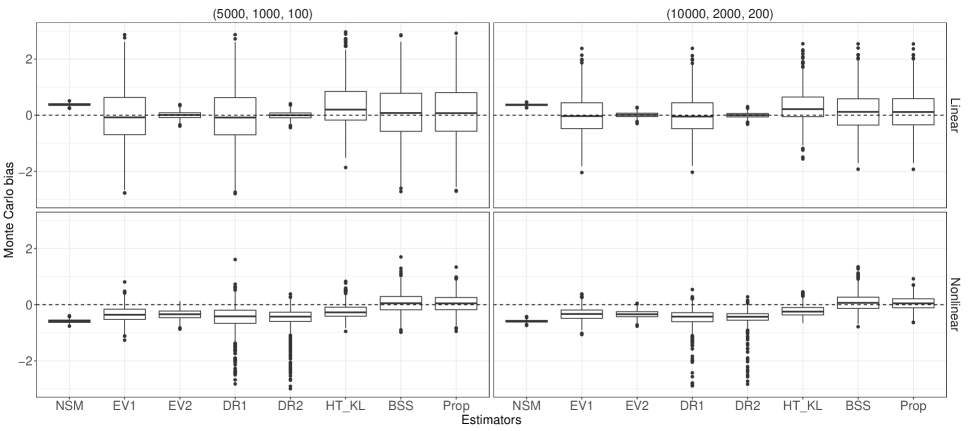
Figure 1: Boxplots for the Monte Carlo bias of different estimators under different setups. The horizontal dashed line corresponds to no bias.

We also compare the computation efficiency of BSS and Prop, and the average computation time required by each estimator is shown in Table 2. Regardless of the model setups, the proposed estimator (4.1) is more computationally efficient than BSS.

Table 2: Computation efficiency of BSS and Prop in terms of average computation time based on 1 000 Monte Carlo simulations (unit: second).

Sizes	Linear			Nonlinear
	BSS	Prop		BSS	Prop
(5 000, 1 000,100)	35.84	7.26		31.11	5.22
(10 000, 2 000,200)	66.59	31.03		137.69	42.47

The coverage rates of the interval estimator with 95% confidence level is also investigated for Prop, and we use Corollary 1 to estimate its variance. Specifically, under Poisson sampling, a plug-in variance estimator is

$$\hat{V}_{prop}=N^{-1}\sum_{i=1}^{N}\delta_{B,i}\pi_{B,i}^{-2}(1-\pi_{B,i})\hat{m}(\bm{x}_{i})^{2}+\hat{\sigma}^{2}N^{-2}\sum_{i=1}^{N}\delta_{A,i}\hat{w}_{i}^{2},$$

where $\hat{m}(\bm{x})$ is obtained by the generalized additive model (Wood,, 2003), and $\hat{\sigma}^{2}$ is the sample variance of $\{y_{i}-\hat{m}(\bm{x}_{i}):i\in A\}$. The coverage rates are close to 0.95 in different model setups, especially when the sample sizes are large.

Table 3: Coverage rate of the interval estimator with 95% confidence level based on 1 000 Monte Carlo simulations.

Model	(5 000, 1 000,100)	(10 000, 2 000,200)
Linear	0.960	0.959
Nonlinear	0.967	0.966

Remark 4.

Although the performance of HT_KL is questionable under the nonlinear model setup, we still consider the performance of its bootstrap variance estimator, and the number of bootstrap replication is $B=200$. We relegate the simulation results to Section S9 of the Supplementary Material, and its performance is satisfactory in terms of relative bias.

6 Application

We compare the performance of the proposed estimator and its alternatives based on a non-probability sample $A$ from the National Health Insurance Sharing Service (NHISS) and a probability sample $B$ from the Korea National Health and Nutrition Examination Survey (KNHANES). National Health Insurance was implemented in 1963 by the Medical Insurance Act, and whole Korean citizens are virtually enrolled in building a healthcare system; see Choi et al., (2015), Jee and Kim, (2019) and the references within for details. KNHANES, on the other hand, is a national survey conducted by the Korea Centers for Disease Control and Prevention since 1998, and it is mainly adopted to assess the health and nutrition status of Korean citizens and provide health-related statistics in Korea. Therefore, the sample of KNHANES is nationally representative, and health-related information, including socioeconomic status, quality of life, health-related behaviors, and healthcare utilization, has been collected; see Kweon et al., (2014) and the references within for details.

In this section, a non-probability sample $A$ contains $n_{A}=20\,000$ elements randomly selected from an NHISS dataset. Demographic information, including age and gender, and health-related information, such as total cholesterol (mg/dL), hemoglobin (HGB), triglyceride (TG), and high-density lipoprotein cholesterol (HDL, mg/dL), is available. The probability sample $B$ is a subset of the blood test results in the 2014 KNHANES, and it was obtained by a multi-stage clustered probability design with sample size $n_{B}=4\,929$. The probability sample $B$ contains the health-related information as that in the non-probability sample. We are interested in estimating the average total cholesterol for different age and gender groups by incorporating information from the two samples.

Even though the average total cholesterol can be estimated by $\hat{N}^{-1}\sum_{i\in B}\pi_{B,i}^{-1}y_{i}$ with $\hat{N}=\sum_{i\in B}\pi_{B,i}^{-1}$, we treat it as unavailable and use it as a benchmark to evaluate the performance of different methods, where $y_{i}$ is the total cholesterol for the $i$th person. That is, we only assume $\{(\bm{x}_{i},y_{i}):i\in A\}$ and $\{(\bm{x}_{i},\pi_{B,i}):i\in B\}$ are available, where $\bm{x}_{i}$ contains the covariates, including HGB, TG and HDL. The population size $N$ is not available, and we use $\hat{N}$ instead. Both samples can be categorized into three age groups, including 20–40, 40–60, and more than 60 years old. Table 4 summarizes the marginal means of the covariates within each age and gender group, and we conclude that there exists a difference for the covariates in the two samples.

Table 4: Marginal means of covariates for the non-probability sample $A$ and the probability sample $B$ for different domains. “20–40” stands for the group with age between 20 and 40, “40–60” for the group with age between 40 and 60, and “60+” for the group with age more than 60.

Gender	Covariate	20–40		40–60		60+
		$A$	$B$	$A$	$B$	$A$	$B$
Female	HDL	63.82	57.28	59.74	54.72	55.20	49.90
	TG	83.72	89.16	110.68	118.31	128.28	137.86
	HGB	12.95	13.06	12.96	13.24	12.89	13.18
Male	HDL	53.14	48.19	51.78	47.12	51.09	46.95
	TG	147.21	160.74	162.87	184.98	133.50	141.65
	HGB	15.47	15.68	15.18	15.41	14.39	14.58

For each age and gender group, consider a regression model (2.1) for the proposed method, and the corresponding benchmark is $\hat{Y}_{BM}=(\sum_{i\in D}\pi_{B,i}^{-1})^{-1}\sum_{i\in D}\pi_{B,i}^{-1}y_{i},$ where $D\subset B$ consists of elements in the group. We also consider NSM, EV2 and DR2 in Section 5 for comparison, and different methods are evaluated by the estimation error $\hat{Y}-\hat{Y}_{BM}$, where $\hat{Y}$ is a specific estimator.

Figure 2 summarizes the estimation errors of different methods for each age and gender group, and we can reach the following conclusions. NSM overestimates the average total cholesterol for each age and gender group, and its performance is questionable. Even though HT_KL performs better than NSM, it is still much worse than EV2, DR2, BSS and Prop. Prop and BBS perform at least as well as EV2 and DR2 in all groups, and they outperform EV2 and DR2 for some groups. For example, in the female group with age 20–40, the estimation errors of Prop and BSS are less than EV2 and DR2, and a similar observation holds for the male group with age 20–40.

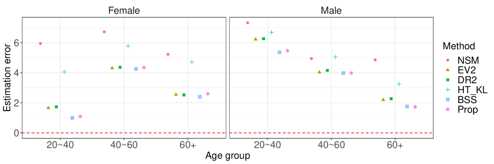
Figure 2: Estimation error of different methods for each age and gender group. “NSM” is the naive sample mean estimator using the non-probability sample, “EV2” is the method considered by Elliott and Valliant, (2017), “DR2” is the one proposed by Chen et al., (2020),“HT_KL” is the estimator in (3.5), “BSS” is the balancing estimator of Wong and Chan, (2018) adopted to survey sampling, and “Prop” is the proposed method.

7 Concluding remarks

We propose a uniform function calibration method to estimate the sampling weights of a non-probability sample based on a probability sample, which is generated by a rejective sampling design. Compared with existing methods, the proposed method does not make any parametric assumption either for the regression model or the response model, so it can be widely adopted in practice. Besides, different from existing works, a KL-divergence-based penalty is proposed to improve the performance of the proposed method. Consistency and the asymptotic normality of the proposed estimator are established under regularity conditions. Numerical results show that the proposed method outperforms its alternatives, especially when both regression and response models are wrongly specified. The proposed method can be viewed as a “soft” calibration method, since we do not require that $S(\hat{\bm{\gamma}},u)=0$ holds for every $u\in\mathcal{H}$. In survey sampling, however, we may would like to achieve “hard” calibration for certain functions of the covariates, it would be an interesting project to incorporate a “hard” calibration component in the proposed objective function.

Supplemental Material for “Functional Calibration under Non-Probability Survey Sampling”

S1 Brief introduction to RKHS

A symmetric bivariate function $K:\mathcal{X}\times\mathcal{X}\to\mathbb{R}$ is a positive semidefinitive kernel function, if for all integer $n\geq 1$ and elements $\{\bm{x}_{1},\ldots,\bm{x}_{n}\}\subset\mathcal{X}$, the $n\times n$ matrix $\bm{M}$ is positive semidefinitive, where $K(\bm{x}_{i},\bm{x}_{j})$ serves as its $(i,j)$-th entry for $i,j=1,\ldots,n$; see Definition 12.6 of Wainwright, (2019) for details.

Let $K(\bm{x},\bm{y})$ be a positive semidefinitive kernel function, and consider a functional space

$${\mathcal{H}}^{\dagger}=\left\{f:f(\cdot)=\sum_{i=1}^{n}\alpha_{j}K(\cdot,\bm{x}_{j})\mbox{ for some }n\geq 1,\{\alpha_{1},\ldots,\alpha_{n}\}\subset\mathbb{R},\{\bm{x}_{1},\ldots,\bm{x}_{n}\}\subset\mathcal{X}\right\}.$$

Then, by Theorem 12.11 of Wainwright, (2019), the complement of ${\mathcal{H}}^{\dagger}$, say $\mathcal{H}$, is an RKHS with the reproducing kernel $K(\bm{x},\bm{y})$.

Furthermore, suppose that the kernel function $K(\bm{x},\bm{y})$ has the following eigen-decomposition:

$$K(\bm{x},\bm{y})=\sum_{j=1}^{\infty}\mu_{j}\psi_{j}(\bm{x})\psi_{j}(\bm{y}),$$

where $\{\mu_{j}:j=1,2,\ldots\}$ are non-negative eigenvalues satisfying $\sum_{j=1}^{\infty}\mu_{j}^{2}<\infty$, and $\{\psi_{j}(\bm{x}):j=1,2,\ldots\}$ are the corresponding eigenfunctions. Then, for any $f\in\mathcal{H}$, there exist $\{c_{j}:j=1,2,\ldots\}$ such that

$$f(\bm{x})=\sum_{j=1}^{\infty}c_{j}\psi_{j}(\bm{x}),$$

and the corresponding norm associated with $\mathcal{H}$ is defined as

$$\lVert f\rVert_{\mathcal{H}}^{2}=\sum_{j=1}^{\infty}c_{j}^{2}/\mu_{j}.$$

See Section 12.2.3 of Wainwright, (2019) and Section 5.8.1 of Hastie et al., (2009) for details.

S2 Numerical solution of the optimization problem

Consider $u(\bm{x})=\sum_{i=1}^{n}\alpha_{i}K(\bm{x}_{i},\cdot)$, and denote $\bm{u}=\bm{M}\bm{\alpha}$, where $\bm{u}=(u(\bm{x}_{1}),\ldots,u(\bm{x}_{n}))^{\mathrm{T}}$, $\bm{\alpha}=(\alpha_{1},\ldots,\alpha_{n})^{\mathrm{T}}$, and $\bm{M}$ is an $n\times n$ Gram matrix with $(i,j)$-th element being $K(\bm{x}_{i},\bm{x}_{j})$. Assume that the eigen-decomposition of $\bm{M}$ is

$$\bm{M}=\begin{pmatrix}\bm{P}_{1}&\bm{P}_{2}\end{pmatrix}\begin{pmatrix}\bm{Q}_{1}&\bm{0}\\ \bm{0}&\bm{Q}_{2}\end{pmatrix}\begin{pmatrix}\bm{P}_{1}^{\mathrm{T}}\\ \bm{P}_{2}^{\mathrm{T}}\end{pmatrix},$$ (S2.1)

where $\bm{Q}_{1}$ is a diagonal matrix consisting the positive eigenvalues, and $\bm{Q}_{2}$ is a zero matrix. Notice that $\bm{Q}_{2}$ may be a null matrix. Then, $S(\bm{\gamma},u)=N^{-2}\bm{\alpha}^{\mathrm{T}}\bm{M}\bm{A}(\bm{\gamma})\bm{M}\bm{\alpha}$ and $\lVert u\rVert_{2}^{2}=n^{-1}\bm{\alpha}^{\mathrm{T}}\bm{M}^{2}\bm{\alpha}$, where $\bm{A}(\bm{\gamma})=\bm{w}(\bm{\gamma})\bm{w}(\bm{\gamma})^{\mathrm{T}}$, and $\bm{w}(\bm{\gamma})=(w_{1}(\bm{\gamma}),\ldots,w_{n}(\bm{\gamma}))^{\mathrm{T}}$. Denote $\bm{\beta}=n^{-1/2}\bm{Q}_{1}\bm{P}_{1}^{\mathrm{T}}\bm{\alpha}$, the inner optimization problem becomes

$$\sup_{\bm{\beta}:\lVert\bm{\beta}\rVert_{2}\leq 1}\bm{\beta}^{\mathrm{T}}\left\{\frac{n}{N^{2}}P_{1}^{\mathrm{T}}A(\bm{\gamma})P_{1}-n\lambda_{1}Q_{1}^{-1}\right\}\bm{\beta}.$$ (S2.2)

Then, we can use a similar procedure in Section 2.3 of Wong and Chan, (2018) to solve the optimization problem (3.3).

S3 Proof of Lemma 1

First, we present a definition of negative association as in Definition 2.1 of Joag-Dev and Proschan, (1983).

Definition 1.

Random variables $X_{1},\ldots,X_{N}$ are said to be negatively associated if for every pair of disjoint subsets $A_{1}$, $A_{2}$ of $\{1,\ldots,N\}$,

$$\mathrm{Cov}\{f_{1}(X_{i},i\in A_{1}),f_{2}(X_{i},i\in A_{2})\}\leq 0,$$ (S3.1)

where $f_{1}$ and $f_{2}$ are increasing functions in every variable.

It can be easily shown that if both $f_{1}$ and $f_{2}$ are decreasing functions in every variable, we still get (S3.1) for negatively associated random variables since $-f_{1}$ and $-f_{2}$ are increasing and $\text{Cov}\{-f_{1}(X_{i},i\in A_{1}),-f_{2}(X_{i},i\in A_{2})\}=\text{Cov}\{f_{1}(X_{i},i\in A_{1}),f_{2}(X_{i},i\in A_{2})\}$.

Lemma S1.

Suppose that Assumption A7 holds. Then, we have

$$E\{\exp(W_{B,i}^{2})\}-1\leq\sigma_{0}^{2},$$

uniformly for $i=1,\ldots,N$, where $W_{B,i}=(\delta_{B,i}\pi_{B,i}^{-1}-1)n_{B}N^{-1}$ and $\sigma_{0}^{2}=\exp\{\max\{1,(C_{B,2}^{-1}-1)^{2},C_{B,1}^{-2}\}\}-1$.

Proof of Lemma S1.

Consider

$$E\{\exp(W_{B,i}^{2})\} = \pi_{B,i}\exp\{(\pi_{B,i}^{-1}-1)^{2}n_{B}^{2}N^{-2}\}+(1-\pi_{B,i})\exp(n_{B}^{2}N^{-2})$$ (S3.2)

$$\leq \pi_{B,i}\exp(\max\{(C_{B,2}^{-1}-1)^{2},C_{B,1}^{-2}\})+(1-\pi_{1})e$$

$$\leq \exp(\max\{1,(C_{B,2}^{-1}-1)^{2},C_{B,1}^{-2}\}),$$

where first inequality holds by Assumption A7. By (S3.2), we have proved Lemma S1. ∎

The next lemma is a straightforward result from Definition 1, so we omit its proof.

Lemma S2.

For any $m\geq 2$ and mutually disjoint subsets $A_{1},\ldots,A_{m}$ of $\{1,\ldots,N\}$ and negatively associated random variables $X_{1},\ldots,X_{N}$, we have

$$E\left\{\prod_{k=1}^{m}f_{k}(X_{i}:i\in A_{k})\right\}\leq\prod_{k=1}^{m}E\left\{f_{k}(X_{i}:i\in A_{k})\right\},$$ (S3.3)

where $f_{1},\ldots,f_{m}$ are decreasing and non-negative functions in every variable.

The next lemma shows a Hoeffding’s inequality (van de Geer,, 2000, Lemma 3.5) under rejective sampling.

Lemma S3.

Suppose Assumption A7 holds. Then, there exist positive constants $C_{B,3}$ and $C_{B,4}$, such that for any $a\geq 0$ and $\{\gamma_{i}:i=1,\ldots,N\}\subset\mathbb{R}$, we have

$$P\left(\left\lvert\sum_{i=1}^{N}W_{B,i}\gamma_{i}\right\rvert\geq a\right)\leq C_{B,3}\exp\left\{-\frac{a^{2}}{C_{B,4}\sum_{i=1}^{N}\gamma_{i}^{2}}\right\},$$ (S3.4)

where $W_{B,i}$ is defined in Lemma S1.

Proof of Lemma S3.

Since the probability sample $B$ is generated by a rejective sampling design, the corresponding sampling indicators are negatively associated by Theorem 3 of Bertail and Clémençon, (2016). Given the sequence $\{\gamma_{i}:i=1,\ldots,N\}$, denote $\mathcal{I}=\{i:\gamma_{i}\geq 0\}$. Then, for any positive constant $a$, we have

$$P\left(\left\lvert\sum_{i=1}^{N}W_{B,i}\gamma_{i}\right\rvert\geq a\right) \leq P\left(\left\lvert\sum_{i\in\mathcal{I}}W_{B,i}\gamma_{i}\right\rvert\geq\frac{a}{2}\right)+P\left(\left\lvert\sum_{i\notin\mathcal{I}}W_{B,i}\gamma_{i}\right\rvert\geq\frac{a}{2}\right)$$

$$\leq P\left(\sum_{i\in\mathcal{I}}W_{B,i}\gamma_{i}\geq\frac{a}{2}\right)+P\left(\sum_{i\in\mathcal{I}}W_{B,i}\gamma_{i}\leq-\frac{a}{2}\right)$$

$$+P\left(\sum_{i\notin\mathcal{I}}W_{B,i}\gamma_{i}\geq\frac{a}{2}\right)+P\left(\sum_{i\notin\mathcal{I}}W_{B,i}\gamma_{i}\leq-\frac{a}{2}\right).$$

Assume $P\left(\left\lvert\sum_{i\in\mathcal{I}}W_{B,i}\gamma_{i}\right\rvert\geq a/2\right)=0$ if $\mathcal{I}=\emptyset$ and $P\left(\left\lvert\sum_{i\notin\mathcal{I}}W_{B,i}\gamma_{i}\right\rvert\geq a/2\right)=0$ if $\mathcal{I}=\{1,\ldots,N\}$.

Without loss of generality, assume that $\mathcal{I}\neq\emptyset$ and $\mathcal{I}\neq\{1,\ldots,N\}$. For any $\beta>0$, we have

$$P\left(\sum_{i\in\mathcal{I}}W_{B,i}\gamma_{i}\geq\frac{a}{2}\right) \leq \exp\left(-\frac{\beta a}{2}\right)E\left\{\exp\left(\beta\sum_{i\in\mathcal{I}}W_{B,i}\gamma_{i}\right)\right\}$$ (S3.6)

$$\leq \exp\left(-\frac{\beta a}{2}\right)\prod_{i\in\mathcal{I}}E\left\{\exp\left(\beta W_{B,i}\gamma_{i}\right)\right\}$$

$$\leq \exp\left\{2(1+\sigma_{0}^{2})\beta^{2}\sum_{i\in\mathcal{I}}\gamma_{i}^{2}-\frac{\beta a}{2}\right\}$$

$$\leq \exp\left\{2(1+\sigma_{0}^{2})\beta^{2}\sum_{i=1}^{N}\gamma_{i}^{2}-\frac{\beta a}{2}\right\},$$

where the first inequality holds by Cramer’s inequality (Athreya and Lahiri,, 2006, Corollary 3.1.5), the second inequality holds by Property P2 of Joag-Dev and Proschan, (1983) and the fact that $\beta\gamma_{i}>0$ for $i\in\mathcal{I}$, the third inequality by Lemma 8.1 of van de Geer, (2000) and Lemma S1, the last inequality holds since $2(1+\sigma_{0}^{2})>0$, and $\sigma_{0}^{2}$ is defined in Lemma S1. If we set

$$\beta=\frac{a}{8(1+\sigma_{0}^{2})\sum_{i=1}^{N}\gamma_{i}^{2}},$$

by (S3.6), we have

$$P\left(\sum_{i\in\mathcal{I}}W_{B,i}\gamma_{i}\geq\frac{a}{2}\right)\leq\exp\left\{-\frac{a^{2}}{32(1+\sigma_{0}^{2})\sum_{i=1}^{N}\gamma_{i}^{2}}\right\}.$$ (S3.7)

Next, for any $\beta>0$, consider

$$P\left(\sum_{i\in\mathcal{I}}W_{B,i}\gamma_{i}\leq-\frac{a}{2}\right) = P\left(\sum_{i\in\mathcal{I}}W_{B,i}\tilde{\gamma}_{i}\geq\frac{a}{2}\right)$$

$$\leq \exp\left(-\frac{\beta a}{2}\right)E\left\{\exp\left(\beta\sum_{i\in\mathcal{I}}W_{B,i}\tilde{\gamma}_{i}\right)\right\}$$

$$\leq \exp\left(-\frac{\beta a}{2}\right)\prod_{i\in\mathcal{I}}E\left\{\exp\left(\beta W_{B,i}\tilde{\gamma}_{i}\right)\right\}$$

where $\tilde{\gamma}_{i}=-\gamma_{i}$, and the last inequality holds by Lemma S2 since $\beta\tilde{\gamma}_{i}\leq 0$ for $i\in\mathcal{I}$. Then, we can use a similar argument leading to (S3.7) to get

$$P\left(\sum_{i\in\mathcal{I}}W_{B,i}\gamma_{i}\leq-\frac{a}{2}\right)\leq\exp\left\{-\frac{a^{2}}{32(1+\sigma_{0}^{2})\sum_{i=1}^{N}\gamma_{i}^{2}}\right\}.$$ (S3.8)

Besides, we can also get

$$P\left(\sum_{i\notin\mathcal{I}}W_{B,i}\gamma_{i}\geq\frac{a}{2}\right)\leq\exp\left\{-\frac{a^{2}}{32(1+\sigma_{0}^{2})\sum_{i=1}^{N}\gamma_{i}^{2}}\right\},$$ (S3.9)

since $\gamma_{i}\leq 0$ for $i\notin\mathcal{I}$.

$$P\left(\sum_{i\notin\mathcal{I}}W_{B,i}\gamma_{i}\leq-\frac{a}{2}\right)=P\left(\sum_{i\notin\mathcal{I}}W_{B,i}\tilde{\gamma}_{i}\geq\frac{a}{2}\right).$$

Then, we can use a similar procedure as (S3.6)–(S3.7) to verify

$$P\left(\sum_{i\notin\mathcal{I}}W_{B,i}\gamma_{i}\leq-\frac{a}{2}\right)\leq\exp\left\{-\frac{a^{2}}{32(1+\sigma_{0}^{2})\sum_{i=1}^{N}\gamma_{i}^{2}}\right\},$$ (S3.10)

since $\tilde{\gamma}_{i}\geq 0$ for $i\notin\mathcal{I}$.

By (LABEL:eq:_prob_12) and (S3.7)–(S3.10), we have proved Lemma S3 with $C_{B,3}=4$ and $C_{B,4}=32(1+\sigma_{0}^{2})$. ∎

Let $\mathcal{H}_{1}=\{u\in\mathcal{H}:\lVert u\rVert_{\mathcal{H}}=1\}$. By Lemma S7 of Wong and Chan, (2018), there exists a constant $R$ such that

$$\sup_{u\in\mathcal{H}_{1}}\lVert u\rVert_{\infty}\leq R.$$ (S3.11)

Denote $H_{\infty}(\epsilon,\mathcal{H}_{1})$ to be the uniform entropy for $\mathcal{H}_{1}$; see Definition 2.3 of van de Geer, (2000) for details about the uniform entropy.

Lemma S4.

Suppose Assumption A4 holds. There exists a constant $C_{B,5}$, such that for any $n_{B}\leq N$ and $S\geq S_{0}$, we have

$$\sum_{s=S_{0}}^{S}2^{-s}RH_{\infty}^{1/2}(2^{-s}(n_{B}N^{-1})^{1/2}R,\mathcal{H}_{1})\leq C_{B,5}N^{1/2}n_{B}^{-1/2},$$ (S3.12)

where $S_{0}=\max\{s:R\leq 2^{-s}n_{B}N^{-1}\leq 2R\}$.

Proof of Lemma S4.

By Assumption A4 and Lemma S6 of Wong and Chan, (2018), there exists a constant $C_{\mathcal{H}}$ such that for $\epsilon>0$,

$$H_{\infty}(\epsilon,\mathcal{H}_{1})\leq C_{\mathcal{H}}\epsilon^{-d/l}.$$ (S3.13)

Consider

$$\sum_{s=S_{0}}^{S}2^{-s}RH_{\infty}^{1/2}(2^{-s}(n_{B}N^{-1})^{1/2}R,\mathcal{H}_{1})$$ (S3.14)

$$= (Nn_{B}^{-1})^{1/2}\sum_{s=S_{0}}^{S}2^{-s}(n_{B}N^{-1})^{1/2}RH_{\infty}^{1/2}(2^{-s}(n_{B}N^{-1})^{1/2}R,\mathcal{H}_{1})$$

$$\leq 2(Nn_{B}^{-1})^{1/2}\int_{0}^{2R}H_{\infty}^{1/2}(\epsilon,\mathcal{H}_{1})\mbox{d}\epsilon$$

$$\leq 2(Nn_{B}^{-1})^{1/2}\frac{C_{\mathcal{H}}^{1/2}(2R)^{1-d/(2l)}}{1-d/(2l)}$$

$$= C_{B,5}(Nn_{B}^{-1})^{1/2},$$

where the second inequality holds by (S3.13) and $C_{B,5}=2^{2-d/(2l)}C_{\mathcal{H}}^{1/2}R^{1-d/(2l)}\{1-d/(2l)\}^{-1}$. Thus, we have proved Lemma S4 by (S3.14). ∎

Lemma S5.

Suppose Assumption A4 and Assumption A7 hold. Then, for all $0\leq\epsilon<\delta$ and $K>1$, there exists $N_{0}=N_{0}(\delta,\epsilon)$, such that for $N\geq N_{0}$, we have

$$P\left[\left\{\sup_{u\in\mathcal{H}_{1}}\left\lvert\frac{1}{n_{B}}\sum_{i=1}^{N}W_{B,i}u(\bm{x}_{i})\right\rvert\geq\delta\right\}\bigcap\left\{\left\lvert\frac{1}{n_{B}}\sum_{i=1}^{N}W_{B,i}\right\rvert\leq K\right\}\right]\leq C_{B,6}\exp\left\{-\frac{n_{B}(\delta-\epsilon)^{2}}{C_{B,6}R^{2}}\right\},$$

where $C_{B,6}$ only depends on $\sigma_{0}^{2}$ defined in Lemma S1.

Proof of Lemma S5.

By (S3.13), there exists a finite $N_{s}$ such that $\{u_{j}^{s}:j=1,\ldots,N_{s}\}$ is a minimal $\{2^{-s}(n_{B}N^{-1})^{1/2}R\}$-covering set of $\mathcal{H}_{1}$ for $s=S_{0},S_{0}+1,\ldots,S$ in terms of the $\lVert\cdot\rVert_{\infty}$ norm, where $S_{0}=\max\{s:R\leq 2^{-s}n_{B}N^{-1}\leq 2R\}$ and $S=\min\{s\geq 1:2^{-s}(n_{B}N^{-1})^{1/2}R\leq\epsilon/(2K)\}$.

By Assumption A7 and Lemma S4, there exists $N_{0}=N_{0}(\delta,\epsilon)$, such that when $N\geq N_{0}$,

$$n_{B}^{1/2}(\delta-\epsilon)\geq\left\{12C_{B,4}^{1/2}R\sum_{s=S_{0}+1}^{S}2^{-s}H_{\infty}^{1/2}(2^{-s}(n_{B}N^{-1})^{1/2}R,\mathcal{H}_{1})\right\}\vee\left\{(1152\log 2)^{1/2}C_{B,4}^{1/2}R\right\},$$ (S3.15)

where $a\vee b=\max\{a,b\}$.

We adopt the notation convenience from Section 3.2 of van de Geer, (2000) and index functions in $\mathcal{H}_{1}$ by $\Theta$: $\mathcal{H}_{1}=\{u_{\theta}:\theta\in\Theta\}$. Then, for any $u_{\theta}\in\mathcal{H}_{1}$, there exists $u_{\theta}^{S}$ such that $\lVert u_{\theta}-u_{\theta}^{S}\rVert_{\infty}\leq\epsilon/(3K)$. Thus, we have

$$\left\lvert\frac{1}{n_{B}}\sum_{i=1}^{N}W_{B,i}\left\{u_{\theta}(\bm{x}_{i})-u_{\theta}^{S}(\bm{x}_{i})\right\}\right\rvert$$ (S3.16)

$$\leq \frac{1}{n_{B}}\left\lvert\sum_{i=1}^{N}\delta_{B,i}\pi^{-1}_{B,i}\frac{n_{B}}{N}\left\{u_{\theta}(\bm{x}_{i})-u_{\theta}^{S}(\bm{x}_{i})\right\}\right\rvert+\frac{1}{N}\left\lvert\sum_{i=1}^{N}\left\{u_{\theta}(\bm{x}_{i})-u_{\theta}^{S}(\bm{x}_{i})\right\}\right\rvert$$

$$\leq \left\{\frac{1}{n_{B}}\left(\sum_{i=1}^{N}\delta_{B,i}\pi^{-1}_{B,i}\frac{n_{B}}{N}\right)+1\right\}\max_{i=1,\ldots,N}\left\lvert\left\{u_{\theta}(\bm{x}_{i})-u_{\theta}^{S}(\bm{x}_{i})\right\}\right\rvert$$

$$\leq \frac{K+2}{3K}\epsilon\leq\epsilon$$

on the event $\{n_{B}^{-1}\lvert\sum_{i=1}^{N}W_{B,i}\rvert\leq K\}$, where the first inequality holds by the definition of $W_{B,i}$ in Lemma S1, the third inequality is due to the fact that the event $\{n_{B}^{-1}\lvert\sum_{i=1}^{N}W_{B,i}\rvert\leq K\}$ implies $\{n_{B}^{-1}\sum_{i=1}^{N}\delta_{B,i}\pi^{-1}_{B,i}n_{B}N^{-1}\leq K+1\}$, and the last inequality holds since $K>1$.

Thus, it is enough to show the exponential inequality for

$$P\left\{\sup_{\theta\in\Theta}\left\lvert\frac{1}{n_{B}}\sum_{i=1}^{N}W_{B,i}u_{\theta}^{S}(\bm{x}_{i})\right\rvert\geq\delta-\epsilon\right\}.$$ (S3.17)

Define $u_{\theta}^{S_{0}}=0$ for $u\in\mathcal{H}_{1}$, and we have $u_{\theta}^{S}=\sum_{s=S_{0}+1}^{S}(u_{\theta}^{s}-u_{\theta}^{s-1})$. For any sequence $\{\eta_{s}:s=S_{0}+1,\ldots,S\}$ satisfying $\sum_{s=S_{0}+1}^{S}\eta_{s}\leq 1$, we have

$$P\left[\sup_{\theta\in\Theta}\left\lvert\frac{1}{n_{B}}\sum_{i=1}^{N}\sum_{s=S_{0}+1}^{S}W_{B,i}\left\{u_{\theta}^{s}(\bm{x}_{i})-u_{\theta}^{s-1}(\bm{x}_{i})\right\}\right\rvert\geq\delta-\epsilon\right]$$ (S3.18)

$$\leq \sum_{s=S_{0}+1}^{S}P\left[\sup_{\theta\in\Theta}\left\lvert\frac{1}{n_{B}}\sum_{i=1}^{N}W_{B,i}\left\{u_{\theta}^{s}(\bm{x}_{i})-u_{\theta}^{s-1}(\bm{x}_{i})\right\}\right\rvert\geq\eta_{s}(\delta-\epsilon)\right]$$

$$\leq \sum_{s=S_{0}+1}^{S}C_{B,3}\exp\left\{2H_{\infty}(2^{-s}(n_{B}N^{-1})^{1/2}R,\mathcal{H}_{1})-\frac{n_{B}\eta_{s}^{2}(\delta-\epsilon)^{2}}{9C_{B,4}2^{-2s}R^{2}}\right\},$$

where the last inequality holds by Lemma S3 and

$$\lVert u_{\theta}^{s}-u_{\theta}^{s-1}\rVert_{\infty} \leq \lVert u_{\theta}^{s}-u_{\theta}\rVert_{\infty}+\lVert u_{\theta}^{s-1}-u_{\theta}\rVert_{\infty}$$

$$\leq 2^{-s}(n_{B}N^{-1})^{1/2}R+2^{-s+1}(n_{B}N^{-1})^{1/2}R\leq 3\{2^{-s}(n_{B}N^{-1})^{1/2}R\}.$$

Now, we consider

$$\eta_{s}=\frac{6RC_{B,4}^{1/2}2^{-s}H_{\infty}^{1/2}(2^{-s}(n_{B}N^{-1})^{1/2}R,\mathcal{H}_{1})}{n_{B}^{1/2}(\delta-\epsilon)}\vee\frac{2^{-s+S_{0}}(s-S_{0})^{1/2}}{8}.$$

Then, by (S3.15) and a similar argument in the proof of Lemma 3.2 of van de Geer, (2000), we can show that

$$\sum_{s=S_{0}+1}^{S}\eta_{s}\leq 1.$$

Thus, we can show that

$$\sum_{s=S_{0}+1}^{S}C_{B,3}\exp\left\{2H_{\infty}(2^{-s}(n_{B}N^{-1})^{1/2}R,\mathcal{H}_{1})-\frac{n_{B}\eta_{s}^{2}(\delta-\epsilon)^{2}}{9C_{B,4}2^{-2s}R^{2}}\right\}$$

$$\leq\sum_{s=S_{0}+1}^{S}C_{B,3}\exp\left\{-\frac{n_{B}\eta_{s}^{2}(\delta-\epsilon)^{2}}{18C_{B,4}2^{-2s}R^{2}}\right\}.$$

Thus, we can use a similar argument in the proof of Lemma 3.2 of van de Geer, (2000) to conclude the proof of Lemma S5 by (S3.15) with $C_{B,6}=\max\{2C_{B,3},C_{B,4}\}$. ∎

By Lemma S3 and setting $K$ sufficient large, we have

$$P\left(\left\lvert\frac{1}{n_{B}}\sum_{i=1}^{N}W_{B,i}\right\rvert>K\right)\leq C_{B,6}\exp\left\{-\frac{n_{B}(\delta-\epsilon)^{2}}{C_{B,6}R^{2}}\right\},$$ (S3.19)

where the related quantities are defined in Lemma S5. Thus, by Lemma S5 and (S3.19), we have

$$P\left\{\sup_{u\in\mathcal{H}_{1}}\left\lvert\frac{1}{n_{B}}\sum_{i=1}^{N}W_{B,i}u(\bm{x}_{i})\right\rvert\geq\delta\right\}$$ (S3.20)

$$\leq P\left[\left\{\sup_{u\in\mathcal{H}_{1}}\left\lvert\frac{1}{n_{B}}\sum_{i=1}^{N}W_{B,i}u(\bm{x}_{i})\right\rvert\geq\delta\right\}\bigcap\left\{\left\lvert\frac{1}{n_{B}}\sum_{i=1}^{N}W_{B,i}\right\rvert\leq K\right\}\right]+P\left(\left\lvert\frac{1}{n_{B}}\sum_{i=1}^{N}W_{B,i}\right\rvert>K\right)$$

$$\leq 2C_{B,6}\exp\left\{-\frac{n_{B}(\delta-\epsilon)^{2}}{C_{B,6}R^{2}}\right\}.$$

Thus, take $C_{B,7}=2C_{B,6}$ and $\epsilon$ sufficiently small, we conclude

$$P\left\{\sum_{u\in\mathcal{H}_{1}}\left\lvert\frac{1}{n_{B}}\sum_{i=1}^{N}W_{B,i}u(\bm{x}_{i})\right\rvert\geq\delta\right\}\leq C_{B,7}\exp\left\{-\frac{n_{B}\delta^{2}}{C_{B,7}R^{2}}\right\}.$$ (S3.21)

Denote

$$S_{N,A}(\bm{\gamma},u) = \left(N^{-1}\sum_{i=1}^{N}\left[\delta_{A,i}\left\{1+\left(\frac{N}{n_{A}}-1\right)r_{i}\right\}-1\right]u(\bm{x}_{i})\right)^{2},$$ (S3.22)

and

$$S_{N,B}(u) = \left\{N^{-1}\sum_{i=1}^{N}(\delta_{B,i}\pi^{-1}_{B,i}-1)u(\bm{x}_{i})\right\}^{2}.$$ (S3.23)

Proof of Lemma 1.

By the fact that $S_{N}(\bm{\gamma}^{\star},u)\leq 2S_{N,A}(\bm{\gamma}^{\star},u)+2S_{N,B}(u),$ we have

$$P\left\{\sup_{u\in\widetilde{\mathcal{H}}_{N}}\frac{n_{B}S_{N}(\bm{\gamma}^{\star},u)}{\lVert u\rVert^{d/l}_{\mathcal{H}}}\geq T^{2}\right\}$$ (S3.24)

$$\leq P\left\{\sup_{u\in\widetilde{\mathcal{H}}_{N}}\frac{n_{B}S_{N,A}(\bm{\gamma}^{\star},u)}{\lVert u\rVert^{d/l}_{\mathcal{H}}}\geq\frac{T^{2}}{4}\right\}+P\left\{\sup_{u\in\widetilde{\mathcal{H}}_{N}}\frac{n_{B}S_{N,B}(u)}{\lVert u\rVert^{d/l}_{\mathcal{H}}}\geq\frac{T^{2}}{4}\right\},$$

where $S_{N,A}(\bm{\gamma},u)$ and $S_{N,B}(u)$ are in (S3.22) and (S3.23). By Assumptions A1–A4, following a similar argument of Lemma S1 of Wong and Chan, (2018), we can show

$$P\left\{\sup_{u\in\widetilde{\mathcal{H}}_{N}}\frac{NS_{N,A}(\bm{\gamma}^{\star},u)}{\lVert u\rVert^{d/l}_{\mathcal{H}}}\geq\frac{T^{2}}{4}\right\}\leq C_{A,3}\exp\left(-\frac{16T^{2}}{C_{A,3}^{2}}\right),$$ (S3.25)

where $C_{A,3}$ is a constant. Since $n_{B}\leq N$, we have

$$P\left\{\sup_{u\in\widetilde{\mathcal{H}}_{N}}\frac{n_{B}S_{N,A}(\bm{r}^{\star},u)}{\lVert u\rVert^{d/l}_{\mathcal{H}}}\geq\frac{T^{2}}{4}\right\} \leq P\left\{\sup_{u\in\widetilde{\mathcal{H}}_{N}}\frac{NS_{N,A}(\bm{r}^{\star},u)}{\lVert u\rVert^{d/l}_{\mathcal{H}}}\geq\frac{T^{2}}{4}\right\}.$$ (S3.26)

By (S3.25)–(S3.26), we have

$$P\left\{\sup_{u\in\widetilde{\mathcal{H}}_{N}}\frac{n_{B}S_{N,A}(\bm{r}^{\star},u)}{\lVert u\rVert^{d/l}_{\mathcal{H}}}\geq\frac{T^{2}}{4}\right\}\leq C_{A,3}\exp\left(-\frac{16T^{2}}{C_{A,3}^{2}}\right).$$ (S3.27)

Next, we investigate the second part on the right hand side of (S3.24). By

$$S_{N,B}(u) = \left[\frac{1}{n_{B}}\sum_{i=1}^{N}W_{B,i}u(\bm{x}_{i})\right]^{2},$$ (S3.28)

where $W_{B,i}$ is defined in Lemma S1.

By (S3.21) and a similar proof for Lemma 8.4 of van de Geer, (2000), there exists a constant $C_{B,8}$ such that

$$P\left\{\sup_{u\in\widetilde{\mathcal{H}}_{N}}\frac{n_{B}S_{N,B}(u)}{\lVert u\rVert^{d/l}_{\mathcal{H}}}\geq\frac{T^{2}}{4}\right\}\leq C_{B,8}\exp\left(-\frac{16T^{2}}{C_{B,8}^{2}}\right).$$ (S3.29)

By (S3.27) and (S3.29), we have validated Lemma 1 by setting $c=C_{A,3}+C_{B,8}$. ∎

S4 Proof of Theorem 1

Recall $n=n_{A}+n_{B}$, and $\lVert u\rVert_{2}^{2}=n^{-1}\sum_{i=1}^{n}u(\bm{x}_{i})^{2}$. Notice that we have assumed $\lVert u\rVert_{\mathcal{H}}<\infty$ for $u\in\mathcal{H}$.

Lemma S6.

Suppose Assumption A4 holds. Then, for $u\in\mathcal{H}$, we have

$$E(\lVert u\rVert_{2}^{2})<\infty,\quad E(\lVert u\rVert_{2}^{4})<\infty.$$

Proof of Lemma S6.

By Lemma S7 of Wong and Chan, (2018), there exists a constant $R$ such that $\sup_{u\in\mathcal{H}_{1}}\lVert u\rVert_{\infty}\leq R$. Thus, for $u\in\mathcal{H}$, $\lVert u\rVert_{\infty}\leq R\lVert u\rVert_{\mathcal{H}}$. Since we have assumed $\lVert u\rVert_{\mathcal{H}}<\infty$ for $u\in\mathcal{H}$ in Section 4, we conclude that $\lVert u\rVert_{\infty}<\infty$, so we have proved Lemma S6.

∎

Denote $u^{\star}=\operatorname*{arg\,max}_{u\in\tilde{\mathcal{H}}_{N}}\{S(\bm{\gamma}^{\star},u)-\lambda_{1}\lVert u\rVert_{\mathcal{H}}\}$, and its existence is shown in Appendix S2, where $\widetilde{\mathcal{H}}_{N}=\{u\in\mathcal{H}:\|u\|_{2}=1\}$. Then, for any $u\in{\mathcal{H}}$, we have

$$S(\hat{\bm{\gamma}},u)-\lambda_{1}\lVert u\rVert_{\mathcal{H}}^{2}-\lambda_{2}Q_{A}(\hat{\bm{\gamma}})\lVert u\rVert_{2}^{2}\leq\{S(\bm{\gamma}^{\star},u^{\star})-\lambda_{1}\lVert u^{\star}\rVert_{\mathcal{H}}^{2}-\lambda_{2}Q_{A}(\bm{\gamma}^{\star})\}\lVert u\rVert_{2}^{2}.$$ (S4.1)

Lemma S7.

Suppose Assumptions A3–A7 hold. If $\lambda_{1}\asymp n_{B}^{-1}$ and $\lambda_{2}\asymp n_{B}^{-1}$, we have $S(\hat{\bm{\gamma}},u)=O_{p}(n_{B}^{-1})\lVert u\rVert_{2}^{2}$ for $u\in\mathcal{H}$.

Proof of Lemma S7.

By (S4.1), we have

$$S(\hat{\bm{\gamma}},u)+\lambda_{1}\lVert u^{\star}\rVert_{\mathcal{H}}^{2}\lVert u\rVert_{2}^{2}+\lambda_{2}Q_{A}(\bm{\gamma}^{\star})\lVert u\rVert_{2}^{2}\leq S(\bm{\gamma}^{\star},u^{\star})\lVert u\rVert_{2}^{2}+\lambda_{1}\lVert u\rVert_{\mathcal{H}}^{2}+\lambda_{2}Q_{A}(\hat{\bm{\gamma}})\lVert u\rVert_{2}^{2}.$$ (S4.2)

By Lemma 1, we can use a similar argument in the proof of Lemma S3 of Wong and Chan, (2018) to reach the following result:

Case (i): Suppose that $S(\bm{\gamma}^{\star},u^{\star})\lVert u\rVert_{2}^{2}$ is the largest on the right-hand side of (S4.2). If $\lVert u\rVert_{2}^{2}>0$, we have $S(\hat{\bm{\gamma}},u)\leq\lambda_{1}^{-d/(2l-d)}O_{p}(n_{B}^{-2l/(2l-d)})\lVert u\rVert_{2}^{2}$. If $\lVert u\rVert_{2}^{2}=0$, we can still get the same result.

Case (ii): Suppose that $\lambda_{1}\lVert u\rVert_{\mathcal{H}}^{2}$ is the largest on the right-hand side of (S4.2). Then, we have $S(\hat{\bm{\gamma}},u)\leq 3\lambda_{1}\lVert u\rVert_{\mathcal{H}}^{2}$.

Case (iii): Suppose that $\lambda_{2}Q_{A}(\hat{\bm{\gamma}})\lVert u\rVert_{2}^{2}$ is the largest on the right-hand side of (S4.2). Then, we have $S(\hat{\bm{\gamma}},u)\leq 3\lambda_{2}Q_{A}(\hat{\bm{\gamma}})\lVert u\rVert_{2}^{2}$.

By (S3.11) and the proof of Lemma S6, $\lVert u\rVert_{2}\leq\lVert u\rVert_{\infty}\leq R\lVert u\rVert_{\mathcal{H}}<\infty$. Then, we have

$$S(\hat{\bm{\gamma}},u)=O_{p}\left[\max\{\lambda_{1}^{-d/(2l-d)}n_{B}^{-2l/(2l-d)}\lVert u\rVert_{2}^{2},\lambda_{1}\lVert u\rVert_{\mathcal{H}}^{2},\lambda_{2}Q_{A}(\hat{\bm{\gamma}})\lVert u\rVert_{2}^{2}\}\right].$$ (S4.3)

By the proposed optimization problem (3.3), $\hat{r}_{i}<\xi_{2}$ for $i=1,\ldots,N$, so $Q_{A}(\hat{\bm{\gamma}})=O_{p}(1)$. Thus, by the conditions on $\lambda_{1}$ and $\lambda_{2}$, we have $S(\hat{\bm{\gamma}},u)=O_{p}(n_{B}^{-1})\lVert u\rVert_{2}^{2}$. Thus, we have complete the proof of Lemma S7. ∎

Based on Lemma S6, we can also use a similar argument as the proof for Lemma S3 of Wong and Chan, (2018) to show that $E\{n_{B}S(\hat{\bm{\gamma}},u)\}<\infty$.

Proof of Theorem 1.

Consider

$$N^{-1}\sum_{i=1}^{N}(\delta_{A,i}\hat{w}_{i}-1)y_{i} = N^{-1}\sum_{i=1}^{N}(\delta_{A,i}\hat{w}_{i}-\delta_{B,i}\pi_{B,i}^{-1})y_{i}+N^{-1}\sum_{i=1}^{N}(\delta_{B,i}\pi_{B,i}^{-1}-1)y_{i}$$ (S4.4)

$$= N^{-1}\sum_{i=1}^{N}(\delta_{A,i}\hat{w}_{i}-\delta_{B,i}\pi_{B,i}^{-1})m_{0}(\bm{x}_{i})+N^{-1}\sum_{i=1}^{N}(\delta_{A,i}\hat{w}_{i}-\delta_{B,i}\pi_{B,i}^{-1})\epsilon_{i}$$

$$+N^{-1}\sum_{i=1}^{N}(\delta_{B,i}\pi_{B,i}^{-1}-1)y_{i}.$$

By Assumption 4 and Lemma S7, we have

$$N^{-1}\sum_{i=1}^{N}(\delta_{A,i}\hat{w}_{i}-\delta_{B,i}\pi_{B,i}^{-1})m_{0}(\bm{x}_{i})=O_{p}(n_{B}^{-1/2}).$$ (S4.5)

Since $\{\epsilon_{i}:i=1,\ldots,N\}$ are independent with the sampling indicators $\{(\delta_{A,i},\delta_{B,i}):i=1,\ldots,N\}$ as well as the weights $\{(\hat{w}_{i},\pi_{B,i}):i=1,\ldots,N\}$, by Assumption A5, we have

$$\mathrm{var}\left\{N^{-1}\sum_{i=1}^{N}\left(\delta_{A,i}\hat{w}_{i}-\delta_{B,i}\pi_{B,i}^{-1}\right)\epsilon_{i}\right\}$$ (S4.6)

$$\leq C_{\sigma,2}E\left\{N^{-2}\sum_{i=1}^{N}\left(\delta_{A,i}\hat{w}_{i}-\delta_{B,i}\pi_{B,i}^{-1}\right)^{2}\right\}$$

$$\leq 2C_{\sigma,2}E\left(N^{-2}\sum_{i=1}^{N}\delta_{B,i}\pi_{B,i}^{-2}\right)+2C_{\sigma,2}E\left(N^{-2}\sum_{i=1}^{N}\delta_{A,i}\hat{w}_{i}^{2}\right).$$

To show the order of (S4.6), we first consider

$$E\left(N^{-2}\sum_{i=1}^{N}\delta_{B,i}\pi_{B,i}^{-2}\right) = N^{-2}\sum_{i=1}^{N}\pi_{B,i}^{-1}$$ (S4.7)

$$\leq C_{B,1}^{-1}N^{-2}\sum_{i=1}^{N}Nn_{B}^{-1}$$

$$= O(n_{B}^{-1}),$$

where the first inequality holds by Assumption A7.

In addition, $n_{A}^{-1}(N-n_{A})\to P(\delta=1)^{-1}P(\delta=0)$ almost surely by strong law of large number. Then, by Assumption A3, there exists a constant $C_{A,4}$, such that $n_{A}^{-1}(N-n_{A})<C_{A,4}$ for $N\geq N_{0}$, where $N_{0}$ is determined by $C_{A,4}$. Then, for $N\geq N_{0}$, since $\hat{w}_{i}=1+(N-n_{A})/n_{A}\hat{r}_{i}$, we have

$$N^{-2}\sum_{i=1}^{N}\delta_{A,i}\hat{w}_{i}^{2} \leq N^{-2}\sum_{i=1}^{N}\delta_{A,i}(1+C_{A,4}\hat{r}_{i})^{2}$$ (S4.8)

$$\leq 2N^{-2}\sum_{i=1}^{N}\delta_{A,i}+2C_{A,4}^{2}N^{-2}\sum_{i=1}^{N}\delta_{A,i}\hat{r}_{i}^{2}$$

$$\leq 2N^{-1}+2C_{A,4}^{2}N^{-2}\sum_{i=1}^{N}\xi_{2}^{2}$$

$$= 2N^{-1}(1+C_{A,4}^{2}\xi_{2}^{2}).$$

Thus, by Assumption A7 and (S4.8), we have

$$E\left(N^{-2}\sum_{i=1}^{N}\delta_{A,i}\hat{w}_{i}^{2}\right)=O(n_{B}^{-1}).$$ (S4.9)

Thus, by (S4.6)–(S4.7) and (S4.9), we have shown that

$$\mathrm{var}\left\{N^{-1}\sum_{i=1}^{N}\left(\delta_{A,i}\hat{w}_{i}-\delta_{B,i}\pi_{B,i}^{-1}\right)\epsilon_{i}\right\}=O(n_{B}^{-1}).$$ (S4.10)

By (S4.4), (S4.5), (S4.10) and Assumption A6, we complete the proof of Theorem 1.

∎

S5 Bootstrap variance estimator

Since the inclusion probabilities are unavailable for the non-probability sample $A$, we consider a bootstrap variance estimator (Kim et al.,, 2019) only taking into consideration the design features associated with the probability sample $B$.

For $b=1,\ldots,B$, let the bootstrap version of (3.5) be

$$\hat{Y}_{N}^{(b)*}=N^{-1}\sum_{i\in A}\hat{\omega}_{i}^{(b)*}y_{i},$$

where $B$ is the number of bootstrap replications, $\hat{\omega}_{i}^{(b)*}=1+(Nn_{A}^{-1}-1)\hat{r}_{i}^{(b)*}$ for $i\in A$, $\hat{\bm{\gamma}}^{(b)*}=(\hat{r}_{1}^{(b)*},\ldots,\hat{r}_{N}^{(b)*})$ with $\hat{r}_{i}^{(b)*}=0$ for $i\notin A$ is obtained by

$$\displaystyle\hat{\bm{\gamma}}^{(b)*}=\operatorname*{arg\,min}_{\xi_{1}\leq r_{i}\leq\xi_{2}}\left[\sup_{u\in{\mathcal{H}}}\left\{\frac{S^{(b)*}(\bm{\gamma},u)}{\lVert u\rVert_{2}^{2}}-\lambda_{1}\frac{\lVert u\rVert_{\mathcal{H}}^{2}}{\lVert u\rVert_{2}^{2}}\right\}-\lambda_{2}Q_{A}(\bm{\gamma})\right],$$

$$\displaystyle S^{(b)*}(\bm{\gamma},u)=\left[N^{-1}\sum_{i=1}^{N}\delta_{A,i}\left\{1+\left(\frac{N}{n_{A}}-1\right)r_{i}\right\}u(\bm{x}_{i})-N^{-1}\sum_{i=1}^{N}\delta_{B,i}d_{B,i}^{(b)*}u(\bm{x}_{i})\right]^{2},$$

the set of bootstrap weights $\{d_{B,i}^{(b)*}:i\in B\}$ satisfies

$$E^{*}\{N^{-1}\sum_{i=1}^{N}\delta_{B,i}d_{B,i}^{(b)*}u(\bm{x}_{i})\}=N^{-1}\sum_{i=1}^{N}\delta_{B,i}\pi_{B,i}^{-1}u(\bm{x}_{i}),$$

$\mathrm{var}^{*}\{N^{-1}\sum_{i=1}^{N}\delta_{B,i}d_{B,i}^{(b)*}u(\bm{x}_{i})\}=\hat{V}\{N^{-1}\sum_{i=1}^{N}\delta_{B,i}\pi_{B,i}^{-1}u(\bm{x}_{i})\}$, $E^{*}(\cdot)$ and $\mathrm{var}^{*}(\cdot)$ are the conditional expectation and variance with respect to the bootstrap procedure given the probability sample $B$, and $\hat{V}\{N^{-1}\sum_{i=1}^{N}\delta_{B,i}\pi_{B,i}^{-1}u(\bm{x}_{i})\}$ is a design-unbiased variance estimator of $N^{-1}\sum_{i=1}^{N}\delta_{B,i}\pi_{B,i}^{-1}u(\bm{x}_{i})$. Then, a bootstrap variance estimator for (3.5) can be the sample variance of $\{\hat{Y}_{N}^{(b)*}:b=1,\ldots,B\}$. The bootstrap variance estimator is reasonable if we can safely ignore the variability with respect to the non-probability sample $A$, for example, when $n_{B}=o_{p}(n_{A})$ by Assumption 3 and Assumption 7

Specifically, if the probability sample $B$ is generated by a Poisson sampling as shown in Section 5, then a design-unbiased variance estimator of $N^{-1}\sum_{i=1}^{N}\delta_{B,i}\pi_{B,i}^{-1}u(\bm{x}_{i})$ is

$$\hat{V}_{B}=\sum_{i\in B}\frac{1-\pi_{B,i}}{\pi_{B,i}^{2}}u^{2}(\bm{x}_{i}).$$

Then, the distribution to generate the bootstrap weights $d_{B,i}^{*}$ can be normal with mean $\pi_{B,i}^{-1}$ and variance $(1-\pi_{B,i})\pi_{B,i}^{-2}$.

S6 Proof of Theorem 2

Lemma S8.

Suppose that Assumption A7 holds. Then, we have

$$N^{-1}\sum_{i=1}^{N}\delta_{B,i}\pi_{B,i}^{-1}=O_{p}(1).$$

Proof of Lemma S8.

Since $P(\delta_{B,i})=\pi_{B,i}$, we have

$$E\left(N^{-1}\sum_{i=1}^{N}\delta_{B,i}\pi_{B,i}^{-1}\right)=1.$$ (S6.1)

Consider

$$\mathrm{var}\left(N^{-1}\sum_{i=1}^{N}\delta_{B,i}\pi_{B,i}^{-1}\right) = N^{-2}\sum_{i=1}^{N}\mathrm{var}(\delta_{B,i}\pi_{B,i}^{-1})+N^{-2}\sum_{i\neq j}\pi_{B,i}^{-1}\pi_{B,j}^{-1}\mathrm{cov}(\delta_{B,i},\delta_{B,j})$$ (S6.2)

$$\leq N^{-2}\sum_{i=1}^{N}\mathrm{var}(\delta_{B,i}\pi_{B,i}^{-1})$$

$$= N^{-2}\sum_{i=1}^{N}(1-\pi_{B,i})\pi_{B,i}^{-1}$$

$$\leq N^{-2}C_{B,1}^{-1}N^{2}n_{B}^{-1}$$

$$= O(n_{B}^{-1}),$$

where the first inequality holds since $\{\delta_{B,i}:i=1,\ldots,N\}$ are negatively associated, and the second inequality holds by Assumption A7. By Assumption A7, $n_{B}^{-1}\to 0$, so we have proved Lemma S8 by (S6.1)–(S6.2). ∎

Lemma S9.

Suppose that Assumptions A1–A8 hold. Then, we have

$$B_{N}^{-1}\sum_{i=1}^{N}(\delta_{A,i}\hat{w}_{i}-\delta_{B,i}\pi_{B,i}^{-1})\epsilon_{i}\to N(0,1),$$

where $B_{N}^{2}=\sum_{i=1}^{N}(\delta_{A,i}\hat{w}_{i}-\delta_{B,i}\pi_{B,i}^{-1})^{2}\sigma_{i}^{2}$. Besides, $B_{N}^{2}\asymp N^{2}n_{B}^{-1}$ in probability.

Proof of Lemma S9.

Denote $\mathcal{A}_{N}=\{(\delta_{A,i},\bm{x}_{i}):i\in A\}\cup\{(\delta_{B,i},\bm{x}_{i}):i\in B\}$. Then, given $\mathcal{A}_{N}$, $B_{N}^{2}$ is the conditional variance of $\sum_{i=1}^{N}(\delta_{A,i}\hat{w}_{i}-1)\epsilon_{i}$.

We first consider the stochastic order of $B_{N}$. On the one hand, we have

$$B_{N}^{2} \leq C_{\sigma,2}\sum_{i=1}^{N}(\delta_{A,i}\hat{w}_{i}-\delta_{B,i}\pi_{B,i}^{-1})^{2}$$ (S6.3)

$$\leq 2C_{\sigma,2}\sum_{i=1}^{B}\delta_{A,i}\hat{w}_{i}^{2}+2C_{\sigma,2}\sum_{i=1}^{N}\delta_{B,i}\pi_{B,i}^{-2}$$

$$= O_{p}(N^{2}n_{B}^{-1}),$$

where the last equality holds by Assumption A7, (S4.7) and (S4.8). On the other hand, consider

$$B_{N}^{2} = \sum_{i=1}^{N}\delta_{A,i}\hat{w}_{i}^{2}\sigma_{i}^{2}-2\sum_{i=1}^{N}\delta_{A,i}\delta_{B,i}\hat{w}_{i}\pi_{B,i}^{-1}\sigma_{i}^{2}+\sum_{i=1}^{N}\delta_{B,i}\pi_{B,i}^{-2}\sigma_{i}^{2}$$ (S6.4)

$$\geq C_{\sigma,1}\sum_{i=1}^{N}\delta_{A,i}\hat{w}_{i}^{2}-2C_{\sigma,1}\max\{\hat{w}_{i}:i=1,\ldots,N\}\sum_{i=1}^{N}\delta_{B,i}\pi_{B,i}^{-1}+C_{\sigma,1}\sum_{i=1}^{N}\delta_{B,i}\pi_{B,i}^{-2}$$

$$\geq C_{\sigma,1}\sum_{i=1}^{N}\delta_{A,i}\hat{w}_{i}^{2}-2C_{\sigma,1}\max\{\hat{w}_{i}:i=1,\ldots,N\}O_{p}(N)+C_{\sigma,1}C_{B,1}^{-2}N^{2}n_{B}^{-1}$$

$$\geq C_{\sigma,1}C_{B,1}^{-2}N^{2}n_{B}^{-1}+o_{p}(N^{2}n_{B}^{-1})$$

where the second inequality holds by Lemma S8, and the last inequality holds by the condition that $\max\{\hat{w}_{i}:i=1,\ldots,N\}$ is bounded since $\hat{\omega}_{i}=1+(Nn_{A}^{-1}-1)\hat{r}_{i}$, $\hat{r}_{i}\leq\xi_{2}$ and $(Nn_{A}^{-1}-1)<C_{A,4}$, where $C_{A,4}$ is discussed in the proof of Theorem 1. Thus, by (S6.3)–(S6.4), we have shown that $B_{N}^{2}\asymp N^{2}n_{B}^{-1}$ in probability.

For any $\eta>0$, consider

$$B_{N}^{-2}\sum_{i=1}^{N}E\{\lvert(\delta_{A,i}\hat{w}_{i}-\delta_{B,i}\pi_{B,i}^{-1})\epsilon_{i}\rvert^{2}I\{\lvert(\delta_{A,i}\hat{w}_{i}-\delta_{B,i}\pi_{B,i}^{-1})\epsilon_{i}\rvert\geq B_{N}\eta\}\mid\mathcal{A}_{N}\}$$ (S6.5)

$$\leq \eta^{\delta}B_{N}^{-2-\delta}\sum_{i=1}^{N}E\{\lvert(\delta_{A,i}\hat{w}_{i}-\delta_{B,i}\pi_{B,i}^{-1})\epsilon_{i}\rvert^{2+\delta}\mid\mathcal{A}_{N}\}$$

$$\leq \eta^{\delta}B_{N}^{-2-\delta}C_{\sigma,1}^{-1}C_{\delta}\max\{\lvert(\delta_{A,i}\hat{w}_{i}-\delta_{B,i}\pi_{B,i}^{-1})\rvert^{\delta}:i=1,\ldots,N\}B_{N}^{2}$$

$$= o_{p}(1),$$

where the second inequality holds by Assumption A5, and last equality holds since $\max\{\lvert(\delta_{A,i}\hat{w}_{i}-\delta_{B,i}\pi_{B,i}^{-1})\rvert^{\delta}:i=1,\ldots,N\}=O(N^{\delta}n_{B}^{-\delta})$ by Assumption A7 and $B_{N}\asymp Nn_{B}^{-1/2}$ in probability. By a similar argument leading to Theorem 4.1 of Yuan et al., (2014), we have proved Lemma S9.

∎

Proof of Theorem 2.

Consider

$$N^{-1}\sum_{i=1}^{N}(\delta_{A,i}\hat{w}_{i}-\delta_{B,i}\pi_{B,i}^{-1})y_{i}-N^{-1}\sum_{i=1}^{N}(\delta_{A,i}\hat{w}_{i}-\delta_{B,i}\pi_{B,i}^{-1})\hat{m}(\bm{x}_{i})$$

$$= N^{-1}\sum_{i=1}^{N}(\delta_{A,i}\hat{w}_{i}-\delta_{B,i}\pi_{B,i}^{-1})\epsilon_{i}+N^{-1}\sum_{i=1}^{N}(\delta_{A,i}\hat{w}_{i}-\delta_{B,i}\pi_{B,i}^{-1})\{m_{0}(\bm{x}_{i})-\hat{m}(\bm{x}_{i})\}.$$

Lemma S9 validates the central limit theorem for the first part of (S6). By Lemma 1 and a similar argument in the proof of Lemma S3 of Wong and Chan, (2018), we can show that

$$N^{-1}\sum_{i=1}^{N}(\delta_{A,i}\hat{w}_{i}-\delta_{B,i}\pi_{B,i}^{-1})\{m(\bm{x}_{i})-\hat{m}(\bm{x}_{i})\}=o_{p}(n_{B}^{-1}).$$ (S6.7)

By the stochastic order of $B_{N}$ in Lemma S9, we have proved Theorem 2. ∎

S7 Proof of Corollary 1

Proof of Corollary 1.

Denote

$$\tilde{\theta} = N^{-1}\sum_{i=1}^{N}\delta_{B,i}\pi_{B,i}^{-1}m(\bm{x}_{i})+N^{-1}\sum_{i=1}^{N}\delta_{A,i}\hat{w}_{i}\{y_{i}-m(\bm{x}_{i})\}$$ (S7.1)

$$= N^{-1}\sum_{i=1}^{N}\delta_{B,i}\pi_{B,i}^{-1}m(\bm{x}_{i})+N^{-1}\sum_{i=1}^{N}\delta_{A,i}\epsilon_{i}.$$

Then, by (S6.7), we have

$$\lvert\hat{\theta}_{prop}-\tilde{\theta}\rvert=\left\lvert N^{-1}\sum_{i=1}^{N}(\delta_{B,i}\pi_{B,i}^{-1}-\delta_{A,i}\hat{w}_{i})\{\hat{m}(\bm{x}_{i})-m(\bm{x}_{i})\}\right\rvert=o_{p}(n_{B}^{-1/2}).$$ (S7.2)

Since the asymptotic order of $\hat{\theta}_{prop}$ is $O_{p}(n_{B}^{-1/2})$ by Assumption A6 and Theorem 2, it is enough to investigate the variance of $\tilde{\theta}$ in (S7.1) by (S7.2).

Consider

$$\mathrm{var}(\tilde{\theta}) = \mathrm{var}\left[E\left\{N^{-1}\sum_{i=1}^{N}\delta_{B,i}\pi_{B,i}^{-1}m(\bm{x}_{i})+N^{-1}\sum_{i=1}^{N}\delta_{A,i}\hat{w}_{i}\epsilon_{i}\mid\mathcal{A}_{N}\right\}\right]$$

$$+E\left[\mathrm{var}\left\{N^{-1}\sum_{i=1}^{N}\delta_{B,i}\pi_{B,i}^{-1}m(\bm{x}_{i})+N^{-1}\sum_{i=1}^{N}\delta_{A,i}\hat{w}_{i}\epsilon_{i}\mid\mathcal{A}_{N}\right\}\right].$$

Since $\epsilon_{i}$ is independent with $\{\delta_{A,i}:i=1,\ldots,N\}$ and $\{\delta_{B,i}:i=1,\ldots,N\}$ by Assumption A6, we have

$$E\left\{N^{-1}\sum_{i=1}^{N}\delta_{B,i}\pi_{B,i}^{-1}m(\bm{x}_{i})+N^{-1}\sum_{i=1}^{N}\delta_{A,i}\hat{w}_{i}\epsilon_{i}\mid\mathcal{A}_{N}\right\}=N^{-1}\sum_{i=1}^{N}\delta_{B,i}\pi_{B,i}^{-1}m(\bm{x}_{i}).$$

Thus, we conclude that

$$\mathrm{var}\left[E\left\{N^{-1}\sum_{i=1}^{N}\delta_{B,i}\pi_{B,i}^{-1}m(\bm{x}_{i})+N^{-1}\sum_{i=1}^{N}\delta_{A,i}\hat{w}_{i}\epsilon_{i}\mid\mathcal{A}_{N}\right\}\right]$$ (S7.4)

$$= \mathrm{var}\left\{N^{-1}\sum_{i=1}^{N}\delta_{B,i}\pi_{B,i}^{-1}m(\bm{x}_{i})\right\}.$$

Next, consider

$$\mathrm{var}\left\{N^{-1}\sum_{i=1}^{N}\delta_{B,i}\pi_{B,i}^{-1}m(\bm{x}_{i})+N^{-1}\sum_{i=1}^{N}\delta_{A,i}\hat{w}_{i}\epsilon_{i}\mid\mathcal{A}_{N}\right\}$$

$$=N^{-1}\sum_{i=1}^{N}\hat{w}_{i}^{2}\sigma^{2}_{i}.$$ (S7.5)

Thus, by (S7.2)–(S7.5), a plug-in variance estimator of $\hat{\theta}_{prop}$ is

$$\hat{V}\left\{N^{-1}\sum_{i=1}^{N}\delta_{B,i}\pi_{B,i}^{-1}\hat{m}(\bm{x}_{i})\right\}+N^{-2}\sum_{i=1}^{N}\delta_{A,i}\hat{w}_{i}^{2}\{y_{i}-\hat{m}(\bm{x}_{i})\}^{2},$$ (S7.6)

where $\hat{V}\left\{N^{-1}\sum_{i=1}^{N}\delta_{B,i}\pi_{B,i}^{-1}\hat{m}(\bm{x}_{i})\right\}$ is a design-based variance of $N^{-1}\sum_{i=1}^{N}\delta_{B,i}\pi_{B,i}^{-1}\hat{m}(\bm{x}_{i})$ treating $\{\hat{m}(\bm{x}_{i}):\delta_{B,i}=1\}$ as non-stochastic. Thus, we have finished the proof of Corollary 1. ∎

S8 Doubly robust estimator by Chen et al., (2020)

Consider a logistic model for the non-probability sample $A$, $\pi_{A,i}=\pi_{A}(\bm{x}_{i};\bm{\theta}_{0})$, where $\mathrm{logit\,}\{\pi_{A}(\bm{x}_{i};\bm{\theta}_{0})\}=\bm{x}_{i}^{\mathrm{T}}\bm{\theta}_{0}$, and $\bm{\theta}_{0}$ is the true parameter. An estimator of $\bm{\theta}_{0}$, say $\hat{\bm{\theta}}$, is obtained by solving

$$\sum_{i\in A}\bm{x}_{i}-\sum_{i\in B}\pi_{B,i}^{-1}\pi_{A}(\bm{x}_{i};\bm{\theta})\bm{x}_{i}=\bm{0}.$$ (S8.1)

The corresponding estimator is termed as “maximum pseudo-likelihood estimator” by Chen et al., (2020).

To overcome the model mis-specification for the sampling mechanism associated with the non-probability sample, Chen et al., (2020) also proposed two double robust estimators by assuming a parametric model for $m_{0}(\bm{x})=m(\bm{x};\bm{\beta}_{0})$, where $\bm{\beta}_{0}$ is an unknown parameter to be estimated. Since missing at random is assumed, we can obtain a consistent estimator of $\bm{\beta}_{0}$, say $\hat{\bm{\beta}}$, using a standard approach. Then, the doubly robust estimators are

$$\hat{Y}_{1}=N^{-1}\sum_{i\in A}\{\pi_{A}(\bm{x}_{i};\hat{\bm{\theta}})\}^{-1}\{y_{i}-m(\bm{x}_{i};\hat{\bm{\beta}})\}+N^{-1}\sum_{i\in B}\pi_{B,i}^{-1}m(\bm{x}_{i};\hat{\bm{\beta}})$$ (S8.2)

and

$$\hat{Y}_{2}=\hat{N}^{-1}\sum_{i\in A}\{\pi_{A}(\bm{x}_{i};\hat{\bm{\theta}})\}^{-1}\{y_{i}-m(\bm{x}_{i};\hat{\bm{\beta}})\}+\hat{N}^{-1}\sum_{i\in B}\pi_{B,i}^{-1}m(\bm{x}_{i};\hat{\bm{\beta}}),$$ (S8.3)

where $\hat{N}=\sum_{i\in A}\{\pi_{A}(\bm{x}_{i};\hat{\bm{\theta}})\}^{-1}$. The only difference between (S8.2) and (S8.3) is that a true population size $N$ is used for (S8.2), but its estimator is used for (S8.3).

S9 Additional simulation result

Under a certain simulation setup, denote $\hat{Y}_{N}^{(m)}$ and $\hat{V}^{(m)}$ to be the HT_KL estimator and its bootstrap variance estimator for the $m$-th Monte Carlo simulation for $m=1,\ldots,M$, where $M=1\,000$ in the simulation study; see Section S5 for details about the bootstrap variance estimator. Let $\hat{V}$ be the sample variance of $\{\hat{Y}_{N}^{(m)}:m=1,\ldots,M\}$. Then, the relative bias of the bootstrap variance estimator is

$$\frac{M^{-1}\sum_{m=1}^{M}\hat{V}^{(m)}-\hat{V}}{\hat{V}}.$$

Table 5 shows the relative bias of the bootstrap variance estimator for HT_KL under different simulation setups. The relative bias of the bootstrap variance estimator is small regardless of the simulation setups. Thus, the variance of HT_KL can be reasonably estimated by bootstrap.

Table 5: Relative bias of the bootstrap variance estimator for HT_KL based on 1 000 Monte Carlo simulations under different simulation setups. The number of replication is $B=200$.

Model	(5 000, 1 000,100)	(10 000, 2 000,200)
Linear	-0.026	0.031
Nonlinear	0.032	0.032

References

• Athreya and Lahiri, (2006) Athreya, K. B. and Lahiri, S. N. (2006). Measure Theory and Probability Theory. Springer, New York.
• Baker et al., (2013) Baker, R., Brick, J. M., Bates, N. A., Battaglia, M., Couper, M. P., Dever, J. A., Gile, K. J., and Tourangeau, R. (2013). Summary report of the AAPOR task force on non-probability sampling. Journal of Survey Statistics and Methodology, 1(2):90–143.
• Beaumont, (2005) Beaumont, J.-F. (2005). Calibrated imputation in surveys under a quasi-model-assisted approach. Journal of the Royal Statistical Society: Series B (Statistical Methodology), 67(3):445–458.
• Bertail et al., (2017) Bertail, P., Chautru, E., and Clémençon, S. (2017). Empirical processes in survey sampling with (conditional) Poisson designs. Scandinavian Journal of Statistics, 44(1):97–111.
• Bertail and Clémençon, (2016) Bertail, P. and Clémençon, S. (2016). Sharp exponential inequalities in survey sampling: conditional Poisson sampling schemes. arXiv:1610.03776, pages 1–25.
• Bethlehem, (2010) Bethlehem, J. (2010). Selection bias in web surveys. International Statistical Review, 78(2):161–188.
• Boistard et al., (2017) Boistard, H., Lopuhaä, H. P., and Ruiz-Gazen, A. (2017). Functional central limit theorems for single-stage sampling designs. Annals of Statistics, 45(4):1728 – 1758.
• Breidt et al., (2005) Breidt, F., Claeskens, G., and Opsomer, J. (2005). Model-assisted estimation for complex surveys using penalised splines. Biometrika, 92(4):831–846.
• Breidt and Opsomer, (2017) Breidt, F. J. and Opsomer, J. D. (2017). Model-assisted survey estimation with modern prediction techniques. Statistical Science, 32(2):190–205.
• Breslow and Wellner, (2007) Breslow, N. E. and Wellner, J. A. (2007). Weighted likelihood for semiparametric models and two-phase stratified samples, with application to Cox regression. Scandinavian Journal of Statistics, 34(1):86–102.
• Brick, (2015) Brick, J. M. (2015). Compositional model inference. In Proceedings of the Survey Research Methods Section, Joint Statistical Meetings, pages 299–307, American Statistical Association, Alexandria, VA.
• Chen et al., (2020) Chen, Y., Li, P., and Wu, C. (2020). Doubly robust inference with nonprobability survey samples. Journal of the American Statistical Association, 115(532):2011–2021.
• Choi et al., (2015) Choi, Y., Kim, J.-H., Yoo, K.-B., Cho, K. H., Choi, J.-W., Lee, T. H., Kim, W., and Park, E.-C. (2015). The effect of cost-sharing in private health insurance on the utilization of health care services between private insurance purchasers and non-purchasers: A study of the Korean health panel survey (2008–2012). BMC Health Services Research, 15(1):1–11.
• Conti, (2014) Conti, P. L. (2014). On the estimation of the distribution function of a finite population under high entropy sampling designs, with applications. Sankhya B, 76(2):234–259.
• Couper, (2000) Couper, M. P. (2000). Web surveys: A review of issues and approaches. Public Opinion Quarterly, 64(4):464–494.
• Couper and Miller, (2008) Couper, M. P. and Miller, P. V. (2008). Web survey methods: Introduction. Public Opinion Quarterly, 72(5):831–835.
• Dever et al., (2008) Dever, J. A., Rafferty, A., and Valliant, R. (2008). Internet surveys: Can statistical adjustments eliminate coverage bias? In Survey Research Methods, volume 2, pages 47–60.
• Dever and Valliant, (2014) Dever, J. A. and Valliant, R. (2014). Estimation with non-probability surveys and the question of external validity. In Proceedings of Statistics Canada Symposium, pages 1–8.
• Deville and Särndal, (1992) Deville, J.-C. and Särndal, C.-E. (1992). Calibration estimators in survey sampling. Journal of the American statistical Association, 87(418):376–382.
• Elliott and Haviland, (2007) Elliott, M. N. and Haviland, A. (2007). Use of a web-based convenience sample to supplement a probability sample. Survey Methodology, 33(2):211–5.
• Elliott and Valliant, (2017) Elliott, M. R. and Valliant, R. (2017). Inference for nonprobability samples. Statistical Science, 32(2):249–264.
• (22) Fuller, W. A. (2009a). Sampling Statistics. Wiley, Hoboken.
• (23) Fuller, W. A. (2009b). Some design properties of a rejective sampling procedure. Biometrika, 96(4):933–944.
• Han and Wang, (2013) Han, P. and Wang, L. (2013). Estimation with missing data: Beyond double robustness. Biometrika, 100(2):417–430.
• Han and Wellner, (2021) Han, Q. and Wellner, J. A. (2021). Complex sampling designs: Uniform limit theorems and applications. Annals of Statistics, 49(1):459 – 485.
• Hastie et al., (2009) Hastie, T., Tibshirani, R., and Friedman, J. (2009). The Elements of Statistical Learning: Data Mining, Inference, and Prediction. Springer, New York, 2nd edition.
• Haziza and Beaumont, (2017) Haziza, D. and Beaumont, J.-F. (2017). Construction of weights in surveys: A review. Statistical Science, 32(2):206–226.