Private measures, random walks, and synthetic data

Abstract.

Differential privacy is a mathematical concept that provides an information-theoretic se curity guarantee. While differential privacy has emerged as a de facto standard for guaranteeing privacy in data sharing, the known mechanisms to achieve it come with some serious limitations. Utility guarantees are usually provided only for a fixed, a priori specified set of queries. Moreover, there are no utility guarantees for more complex—but very common—machine learning tasks such as clustering or classification. In this paper we overcome some of these limitations. Working with metric privacy, a powerful generalization of differential privacy, we develop a polynomial-time algorithm that creates a private measure from a data set. This private measure allows us to efficiently construct private synthetic data that are accurate for a wide range of statistical analysis tools. Moreover, we prove an asymptotically sharp min-max result for private measures and synthetic data for general compact metric spaces. A key ingredient in our construction is a new superregular random walk, whose joint distribution of steps is as regular as that of independent random variables, yet which deviates from the origin logarithmically slowly.

1. Introduction

1.1. Motivation

The right to privacy is enshrined in the Universal Declaration of Human Rights [7]. However, as artificial intelligence is more and more permeating our daily lives, data sharing is increasingly locking horns with data privacy concerns. Differential privacy (DP), a probabilistic mechanism that provides an information-theoretic privacy guarantee, has emerged as a de facto standard for implementing privacy in data sharing [23]. For instance, DP has been adopted by several tech companies [21] and will also be used in connection with the release of the Census 2020 data [3, 2].

Yet, current embodiments of DP come with some serious limitations [18, 26, 52]:

1. Utility guarantees are usually provided only for a fixed set of queries. This means that either DP has to be used in an interactive scenario or the queries have to specified in advance.

2. There are no utility guarantees for more complex—but very common—machine learning tasks such as clustering or classification.

3. DP can suffer from a poor privacy-utility tradeoff, leading to either insufficient privacy protection or to data sets of rather low utility, thereby making DP of limited use in many applications [18].

Another approach to enable privacy in data sharing is based on the concept of synthetic data [9]. The goal of synthetic data is to create a dataset that maintains the statistical properties of the original data while not exposing sensitive information. The combination of differential privacy with synthetic data has been suggested as a best-of-both-world solutions [24, 9, 31, 35, 13]. While combining DP with synthetic data can indeed provide more flexibility and thereby partially address some of the issues in (i), in and of itself it is not a panacea for the aforementioned problems.

One possibility to construct differentially private synthetic datasets that are not tailored to a priori specified queries is to simply add independent Laplacian noise to each data point. However, the amount noise that has to be added to achieve sufficient DP is too large with respect to maintaining satisfactory utility even for basic counting queries [53], not to mention more sophisticated machine learning tasks.

This raises the fundamental question whether it is even possible to construct in a numerically efficient manner differentially private synthetic data that come with rigorous utility guarantees for a wide range of (possibly complex) queries, while achieving a favorable privacy-utility tradeoff? In this paper we will answer this question to the affirmative.

1.2. A private measure

A main objective of this paper is to construct a private measure on a given metric space $(T,\rho)$. Namely, we design an algorithm that transforms a probability measure $\mu$ on $T$ into another probability measure $\nu$ on $T$, and such that this transformation is both private and accurate.

For clarity, let us first consider the special case of empirical measures, where our goal can be understood as creating differentially private synthetic data. Specifically, we are looking for a computationally tractable algorithm that transforms true input data $X=(X_{1},\ldots,X_{n})\in T^{n}$ into synthetic output data $Y=(Y_{1},\ldots,Y_{m})\in T^{m}$ for some $m$, and which is $\varepsilon$-differentially private (see Definition 2.1) and such that the empirical measures

$$\mu_{X}=\frac{1}{n}\sum_{i=1}^{n}\delta_{X_{i}}\quad\text{and}\quad\mu_{Y}=\frac{1}{m}\sum_{i=1}^{m}\delta_{Y_{i}}$$

are close to each other in the Wasserstein 1-metric (recalled in Section 2.2.2):

$$\operatorname{\mathbb{E}}W_{1}\left(\mu_{X},\mu_{Y}\right)\leq\gamma,$$ (1.1)

where $\gamma>0$ is as small as possible.

The main result of this paper is a computationally effective private algorithm whose accuracy $\gamma$ that is expressed in terms of the multiscale geometry of the metric space $(T,\rho)$. A consequence of this result, Theorem 9.6, states that if the metric space has Minkowski dimension $d\geq 1$, then, ignoring the dependence on $\varepsilon$ and lower-order terms in the exponent, we have

$$\operatorname{\mathbb{E}}W_{1}\left(\mu_{X},\mu_{Y}\right)\sim n^{-1/d}$$ (1.2)

The dependence on $n$ is optimal and quite intuitive. Indeed, if the true data $X$ consists of $n$ i.i.d. random points chosen uniformly from the unit cube $T=[0,1]^{d}$, then the average spacing between these points is of the order $n^{-1/d}$. So our result shows that privacy can be achieved by a microscopic perturbation, one whose magnitude is roughly the same as the average spacing between the points.

Our more general result, Theorem 7.2, holds for arbitrary compact metric spaces $(T,\rho)$ and, more importantly, for general input measures (not just empirical ones). To be able to work in such generality, we employ the notion of metric privacy which reduces to differential privacy when we specialize to empirical measures (Section 2.1).

1.3. Uniform accuracy over Lipschitz statistics

The choice of the Wasserstein 1-metric to quantify accuracy ensures that all Lipschitz statistics are preserved uniformly. Indeed, by Kantorovich-Rubinstein duality theorem, (1.1) yields

$$\operatorname{\mathbb{E}}\sup_{f}\Big{|}\frac{1}{n}\sum_{i=1}^{n}f(X_{i})-\frac{1}{m}\sum_{i=1}^{m}f(Y_{i})\Big{|}\leq\gamma$$ (1.3)

where the supremum is over all $1$-Lipschitz functions $f\mathrel{\mathop{\mathchar 58\relax}}T\to\mathbb{R}$.

Standard private synthetic data generation methods that come with rigorous accuracy guarantees do so with respect to a predefined set of linear queries, such as low-dimensional marginals, see e.g. [8, 44, 22, 13]. While this may suffice in some cases, there is no assurance that the synthetic data behave in the same way as the original data under more complex, but frequently employed, machine learning techniques. For instance, if we want to apply a clustering method to the synthetic data, we cannot be sure that the results we get are close to those for the true data. This can drastically limit effective and reliable analysis of synthetic data.

In contrast, since the synthetic data constructed via our proposed method satisfy a uniform bound (1.3), this provides data analysts with a vastly increased toolbox of machine learning methods for which one can expect outcomes that are similar for the original data and the synthetic data.

As concrete examples let us look at two of the most common tasks in machine learning, namely clustering and classification. While not every clustering method will satisfy a Lipschitz property, there do exist Lipschitz clustering functions that achieve state-of-the-art results, see e.g. [32, 55]. Similarly, there is distinct interest in Lipschitz function based classifiers, since they are more robust and less susceptible to adversarial attacks. This includes conventional classification methods such as support vector machines [51] as well as classifiers based on Lipschitz neural networks [50, 10]. These are just a few examples of complex machine learning tools that can be reliably applied to the synthetic data constructed via our private measure algorithm. Moreover, since our results hold for general compact metric spaces, this paves the way for creating private synthetic data for a wide range of data types. We will present a detailed algorithmic and numerical investigation of the proposed method in a forthcoming paper.

1.4. A superregular random walk

The most popular way to achieve privacy is by adding random noise, typically either by adding an appropriate amount of Laplacian noise or Gaussian noise (these methods are aptly referred to as Laplacian mechanism and Gaussian mechanism, respectively [23]). We, too, can try to make a probability measure $\mu$ on $T$ private by discretizing $T$ (replacing it with a finite set of points) and then adding random noise to the weights of the points. Going this route, however, yields suboptimal results. For example, it is not difficult to check that if $T$ is the interval $[0,1]$, the accuracy of the Laplacian mechanism can not be better than $n^{-1/2}$, which is suboptimal compared to optimal accuracy $n^{-1}$ in (1.2).

This loss of accuracy is caused by the accumulation of additive noise. Indeed, adding $n$ independent random variables of unit variance produces noise of the order $n^{1/2}$. This prompts a basic probabilistic question: can we construct $n$ random variables that are “close” to being independent, but whose partial sums cancel more perfectly than those of independent random variables? We answer this question affirmatively in Theorem 3.1, where we construct random variables $Z_{1},\ldots,Z_{n}$ whose joint distribution is as regular as that of i.i.d. Laplacian random variables, yet whose partial sums grow logarithmically as opposed to $n^{1/2}$:

$$\operatorname{\mathbb{E}}\max_{1\leq k\leq n}\mathinner{\!\left\lvert Z_{1}+\cdots+Z_{k}\right\rvert}=O(\log^{2}n).$$

One can think of this as a random walk that is locally similar to the one with i.i.d. steps, but globally is much more bounded. Our construction is a nontrivial modification of Lévy’s construction of Brownian motion. It may be interesting and useful beyond applications to privacy.

1.5. Comparison to existing work

The numerically efficient construction of accurate differentially private synthetic data is highly non-trivial. As case in point, Ullman and Vadhan [45] showed (under standard cryptographic assumptions) that in general it is NP-hard to make private synthetic Boolean data which approximately preserve all two-dimensional marginals. There exists a substantial body of work for generating privacy-preserving synthetic data, cf. e.g. [4, 15, 1, 17, 36], but—unlike our work—without providing any rigorous privacy or accuracy guarantees. Those papers on synthetic data that do provide rigorous guarantees are limited to accuracy bounds for a finite set of a priori specified queries, see for example [8, 12, 44, 22, 13, 14], see also the tutorial [46]. As discussed before, this may suffice for specific purposes, but in general severely limits the impact and usefulness of synthetic data. In contrast, the present work provides accuracy guarantees for a wide range of machine learning techniques. Furthermore, our our results hold for general compact metric spaces, as we establish metric privacy instead of just differential privacy.

A special example of the topic investigated in this paper is the publication of differentially private histograms, which is a well studied problem in the privacy literature, see e.g. [27, 40, 37, 54, 53, 38, 56, 2] and Chapter 4 in [34]. In the specific context of histograms, the Haar function based approach to construct a superregular random walk proposed in our paper is related to the wavelet-based method [53] and to other hierarchical histogram partitioning methods [27, 40, 56]. Like our approach, [27, 53] obtain consistency of counting queries across the hierarchical levels, owing to the specific way that noise is added. Also, the accuracy bounds obtained in [27, 53] are similar to ours, as they are also polylogarithmic (although we are able to obtain a smaller exponent). There are, however, several key differences. While our approach gives a convenient way to generate accurate and differentially private synthetic data $Y$ from true data $X$, the methods of the aforementioned papers are not suited to create synthetic data. Instead, these methods release answers to queries. Moreover, accuracy is proven for just a single given range query and not simultaneously for all queries like we do. This limitation makes it impossible to create accurate synthetic data with the algorithms in [27, 53]. Moreover, unlike the aforementioned papers, our work allows the data to be quite general, since we prove metric privacy and not just differential privacy. Furthermore, our results apply to multi-dimensional data, and are not limited to the one-dimensional setting.

There exist several papers on the private estimation of density and other statistical quantities [28, 19], and sampling from distributions in a private manner is the topic of [41]. While definitely interesting, that line of work is not concerned with synthetic data, and thus there is little overlap with this work.

1.6. The architecture of the paper

The remainder of this paper is organized as follows. We introduce some background material and notation in Section 2, such as the concept of metric privacy which generalizes differential privacy. In Section 3 we construct a superregular random walk (Theorem 3.1). We analyze metric privacy in more detail in Section 4, where we also provide a link from the general private measure problem to private synthetic data (Lemma 4.1). In Section 5 we use the superregular random walk to construct a private measure on the interval $[0,1]$ (Theorem 5.4). In Section 6 we use a link between the Traveling Salesman Problem and minimum spanning trees to devise a folding technique, which we apply in Section 7 to “fold” the interval into a space-filling curve to construct a private measure on a general metric space (Theorem 7.2). Postprocessing the private measure with quantization and splitting, we then generate private synthetic data in a general metric space (Corollary 7.4). In Section 8 we turn to lower bounds for private measures (Theorem 8.5) and synthetic data (Theorem 8.6) on a general metric space. We do this by employing a technique of Hardt and Talwar, which we present in a Proposition 8.1 that identifies general limitations for synthetic data. In Section 9 we illustrate our general results on a specific example of a metric space: the Boolean cube $[0,1]^{d}$. We construct a private measure (Corollary 9.1) and private synthetic data (Corollary 9.2) on the cube, and show near optimality of these results in Corollary 9.3 and Corollary 9.4, respectively. Results similar to the ones for the $d$-dimensional cube hold for arbitrary metric space of Minkowski dimension $d$. For any such space, we prove an asymptotically sharp min-max results for private measures (Theorem 9.5) and synthetic data (Theorem 9.5).

2. Background and Notation

The motivation behind the concept of differential privacy is the desire to protect an individual’s data, while publishing aggregate information about the database [23]. Adding or removing the data of one individual should have a negligible effect on the query outcome, as formalized in the following definition.

Definition 2.1 (Differential Privacy [23]).

A randomized algorithm ${\mathcal{M}}$ gives $\varepsilon$-differential privacy if for any input databases $D$ and $D^{\prime}$ differing on at most one element, and any measurable subset $S\subseteq\operatorname{range}({\mathcal{M}})$, we have

$$\frac{\mathbb{P}\left\{{\mathcal{M}}(D)\in S\rule{0.0pt}{8.53581pt}\right\}}{\mathbb{P}\left\{{\mathcal{M}}(D^{\prime})\in S\rule{0.0pt}{8.53581pt}\right\}}\leq\exp(\varepsilon),$$

where the probability is with respect to the randomness of ${\mathcal{M}}$.

2.1. Defining metric privacy

While differential privacy is a concept of the discrete world (where datasets can differ in a single element), it is often desirable to have more freedom in the choice of input data. The following general notion (which seems to be known under slightly different, and somewhat less general, versions, see e.g. [5] and the references therein) extends the classical concept of differential privacy.

Definition 2.2 (Metric privacy).

Let $(T,\rho)$ be a compact metric space and $E$ be a measurable space. A randomized algorithm $\mathcal{A}\mathrel{\mathop{\mathchar 58\relax}}T\to E$ is called $\alpha$-metrically private if, for any inputs $x,x^{\prime}\in T$ and any measurable subset $S\subset E$, we have

$$\frac{\mathbb{P}\left\{\mathcal{A}(x)\in S\rule{0.0pt}{8.53581pt}\right\}}{\mathbb{P}\left\{\mathcal{A}(x^{\prime})\in S\rule{0.0pt}{8.53581pt}\right\}}\leq\exp\left(\alpha\,\rho(x,x^{\prime})\right).$$ (2.1)

To see how this metric privacy encompasses differential privacy, consider a product space $T=\mathcal{X}^{n}$ and equip it with the Hamming distance

$$\rho_{H}(x,x^{\prime})=\mathinner{\!\left\lvert\{i\in[n]\mathrel{\mathop{\mathchar 58\relax}}\;x_{i}\neq x^{\prime}_{i}\}\right\rvert}.$$ (2.2)

The $\alpha$-differentially privacy of an algorithm $\mathcal{A}\mathrel{\mathop{\mathchar 58\relax}}\mathcal{X}^{n}\to E$ can be expressed as

$$\frac{\mathbb{P}\left\{\mathcal{A}(x)\in S\rule{0.0pt}{8.53581pt}\right\}}{\mathbb{P}\left\{\mathcal{A}(x^{\prime})\in S\rule{0.0pt}{8.53581pt}\right\}}\leq\exp\left(\alpha\right)\quad\text{whenever }\rho_{H}(x,x^{\prime})\leq 1.$$ (2.3)

Note that (2.3) is equivalent to (2.1) for $\rho=\rho_{H}$. Obviously, (2.1) implies (2.3). The converse implication can be proved by replacing one coordinate of $x$ by the corresponding coordinate of $x^{\prime}$ and applying (2.3) $\rho_{H}(x,x^{\prime})$ times, then telescoping. Let us summarize:

Lemma 2.3 (MP vs. DP).

Let $\mathcal{X}$ be an arbitrary set. Then an algorithm $\mathcal{A}\mathrel{\mathop{\mathchar 58\relax}}\mathcal{X}^{n}\to E$ is $\alpha$-differentially private if an only if $\mathcal{A}$ is $\alpha$-metrically private with respect to the Hamming distance (2.2) on $\mathcal{X}^{n}$.

Unlike differential privacy, metric privacy goes beyond product spaces, and thus allows the data to be quite general. In this paper, for example, the input data are probability measures. Moreover, metric privacy does away with the assumption that the data sets $D,D^{\prime}$ be different in a single element. This assumption is sometimes too restrictive: general measures, for example, do not break down into natural single elements.

2.2. Distances between measures

This paper will use three classical notions of distance between measures.

2.2.1. Total variation

The total variation (TV) norm [20, Section III.1] of a signed measure $\mu$ on a measurable space $(\Omega,\mathcal{F})$ is defined as

$$\mathinner{\!\left\lVert\mu\right\rVert}_{\mathrm{TV}}=\frac{1}{2}\sup_{\Omega=\cup_{i}A_{i}}\sum_{i}\mathinner{\!\left\lvert\mu(A_{i})\right\rvert}$$ (2.4)

where the supremum is over all partitions $\Omega$ into countably many parts $A_{i}\in\mathcal{F}$. If $\Omega$ is countable, we have

$$\mathinner{\!\left\lVert\mu\right\rVert}_{\mathrm{TV}}=\frac{1}{2}\sum_{\omega\in\Omega}\mathinner{\!\left\lvert\mu(\{\omega\})\right\rvert}.$$ (2.5)

The TV distance between two probability measures $\mu$ and $\nu$ is defined as the TV norm of the signed measure $\mu-\nu$. Equivalently,

$$\mathinner{\!\left\lVert\mu-\nu\right\rVert}_{\mathrm{TV}}=\sup_{A\in\mathcal{F}}\mathinner{\!\left\lvert\mu(A)-\nu(A)\right\rvert}.$$

2.2.2. Wasserstein distance

Let $(\Omega,\rho)$ be a bounded metric space. We define the Wasserstein 1-distance (henceforth simply referred to as Wasserstein distance) between probability measures $\mu$ and $\nu$ on $\Omega$ as [49]

$$W_{1}(\mu,\nu)=\inf_{\gamma}\int_{\Omega\times\Omega}\rho(x,y)\,d\gamma(x,y)$$ (2.6)

where the infimum is over all couplings $\gamma$ of $\mu$ and $\nu$, or probability measures on $\Omega\times\Omega$ whose marginals on the first and second coordinates are $\mu$ and $\nu$, respectively. In other words, $W_{1}(\nu,\mu)$ minimizes the transportation cost between the “piles of earth” $\mu$ and $\nu$.

The Kantorovich-Rubinstein duality theorem [49] gives an equivalent representation:

$$W_{1}(\mu,\nu)=\sup_{\mathinner{\!\left\lVert h\right\rVert}_{\mathrm{Lip}}\leq 1}\left(\int h\,d\mu-\int h\,d\nu\right)$$

where the supremum is over all continuous, $1$-Lipschitz functions $h\mathrel{\mathop{\mathchar 58\relax}}\Omega\to\mathbb{R}$.

For probability measures $\mu$ and $\nu$ on $\mathbb{R}$, the Wasserstein distance has the following representation, according to Vallender [47]:

$$W_{1}(\mu,\nu)=\mathinner{\!\left\lVert F_{\mu}-F_{\nu}\right\rVert}_{L^{1}(\mathbb{R})}.$$ (2.7)

Here $F_{\mu}(x)=\mu\left((-\infty,x]\right)$ is the cumulative distribution function of $\mu$, and similarly for $F_{\nu}(x)$.

Vallender’s identity (2.7) can be used to define Wasserstein distance for signed measures on $\mathbb{R}$. Moreover, for signed measures on $[0,1]$, the Wasserstein distance defined this way is always finite, and it defines a pseudometric.

3. A superregular random walk

The classical random walk with independent steps of unit variance is not bounded: it deviates from the origin at the expected rate $\sim n^{1/2}$. Surprisingly, there exists a random walk whose joint distribution of steps is as regular as that of independent Laplacians, yet that deviates from the origin logarithmically slowly.

Theorem 3.1 (A superregular random walk).

For every $n\in\mathbb{N}$, there exists a probability density of the form $f(z)=\frac{1}{\beta}e^{-V(z)}$ on $\mathbb{R}^{n}$ that satisfies the following two properties.

1. (Regularity): the potential $V$ is $1$-Lipschitz in the $\ell^{1}$ norm, i.e.

   $$\mathinner{\!\left\lvert V(x)-V(y)\right\rvert}\leq\mathinner{\!\left\lVert x-y\right\rVert}_{1}\quad\text{for all }x,y\in\mathbb{R}^{n}.$$ (3.1)

2. (Boundedness): a random vector $Z=(Z_{1},\ldots,Z_{n})$ distributed according to the density $f$ satisfies

   $$\operatorname{\mathbb{E}}\max_{1\leq k\leq n}\mathinner{\!\left\lvert Z_{1}+\cdots+Z_{k}\right\rvert}\leq C\log^{2}n,$$ (3.2)

   and

   $$\max_{1\leq k\leq n}\operatorname{\mathbb{E}}\mathinner{\!\left\lvert Z_{1}+\cdots+Z_{k}\right\rvert}\leq C\log^{\frac{3}{2}}n,$$ (3.3)

   where $C>0$ is a universal constant.

3.1. Heuristics

The first candidate for the random walk could be a discretization of the standard Brownian motion on the interval $[0,1]$. The reflection principle yields the boundedness property in the theorem, even without any logarithmic loss. However, the regularity property fails miserably.

To achieve regularity, we would like to grant Brownian motion more freedom. This will be done by modifying Levy’s construction of the Brownian motion. In this construction, the path of a Brownian motion on an interval $[0,n]$ is defined as a random series with respect to the Schauder basis of the space of continuous functions, see also [11, Section IX.1].

To that end, we recall the definition of the Schauder basis of triangular functions of $C[0,1]$. Let $I_{1}$ be the semi-open interval $[0,1)$ and $N_{q}$ the set of all integers $j$ such that $2^{q-1}\leq j<2^{q}$. For any integer $j$ there exists a unique pair of integers $(q_{j},p_{j})$ such that $j=2^{q_{j}}+p_{j}$ where $0\leq p_{j}\leq 2^{q_{j}-1}-1$. Let

$$I_{j}=\Big{\{}t\mathrel{\mathop{\mathchar 58\relax}}\frac{p_{j}}{2^{q_{j}-1}}\leq t<\frac{p_{j}+1}{2^{q_{j}-1}}\Big{\}},\quad t_{j}=\frac{2p_{j}+1}{2^{q_{j}}},$$

and define $\bar{\phi}_{1}(t)=t$ for $t\in I_{1}$ and

$$\bar{\phi}_{j}=\begin{cases}2^{q_{j}}\Big{(}t-\frac{p_{j}}{2^{q_{j}-1}}\Big{)}&\text{for $t\in I_{2j}$},\\ 2^{q_{j}}\Big{(}\frac{p_{j}+1}{2^{q_{j}-1}}-t\Big{)}&\text{for $t\in I_{2j+1}$},\\ 0&\text{otherwise}.\end{cases}$$

The modification of this definition from $C[0,1]$ to $C[0,n]$ is obvious by dilation: $\phi_{j}(t)=\bar{\phi}_{j}(t/n)$.

Thus, the basis functions $\phi_{j}$ are defined by levels $\ell=0,1,2,\ldots$. At level $\ell=0$, we have two functions $\phi_{1}$ and $\phi_{2}$, and each level $\ell\geq 1$ contains $2^{\ell}$ functions $\phi_{j}$ supported in disjoint intervals of length $n/2^{\ell}$. Throughout this section, $\ell(j)$ will denote the level the function $\phi_{j}$ belongs to, e.g. $\ell(1)=\ell(2)=0$, $\ell(3)=\ell(4)=1$, $\ell(5)=\ell(6)=\ell(7)=\ell(8)=2$, etc. See Figure 1 for an illustration of these functions.

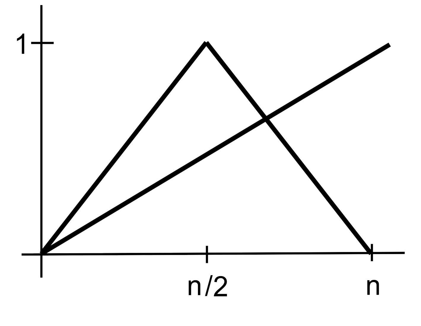
Level 0: $\phi_{1},\phi_{2}$

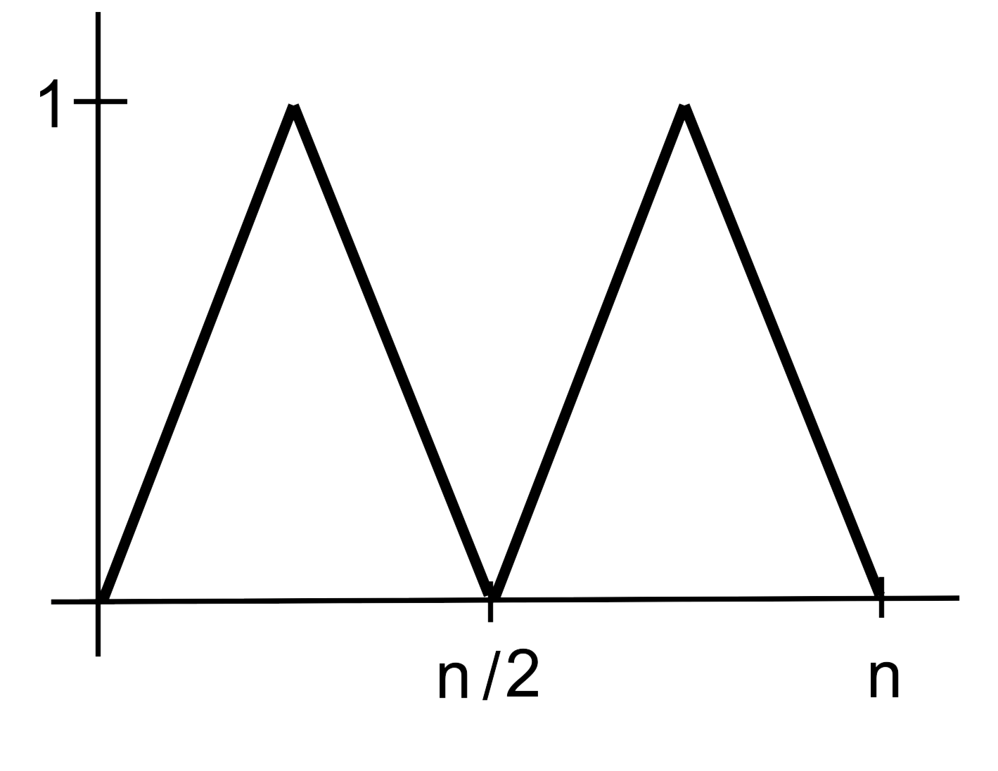
Level 1: $\phi_{3},\phi_{4}$

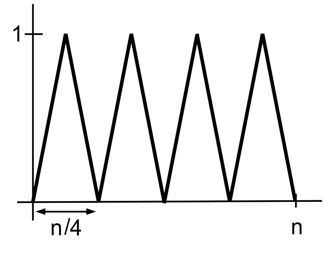
Level 2: $\phi_{5},\dots,\phi_{8}$

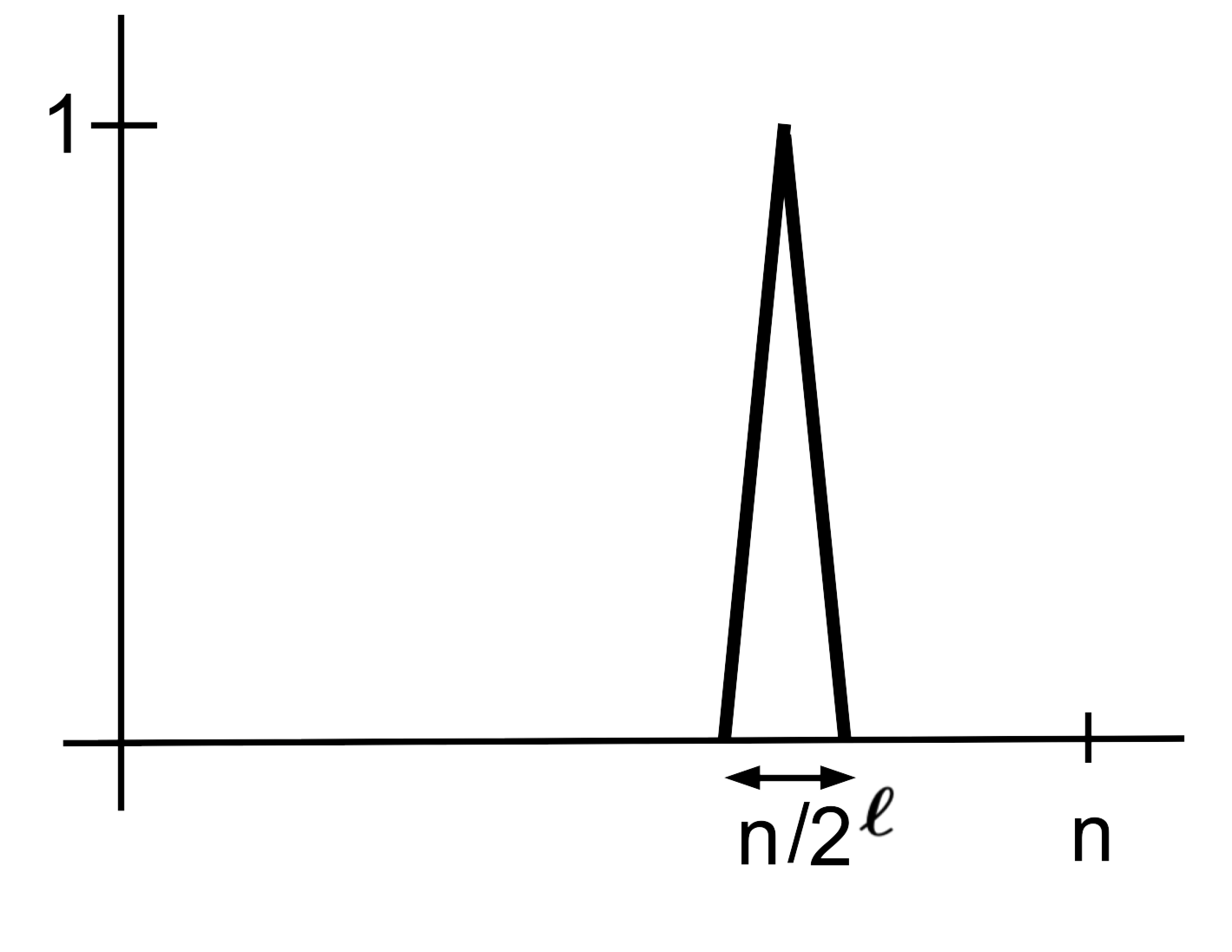
Level $\ell$

…

Figure 1. Schauder basis

Lévy’s definition of the standard Brownian motion on the interval $[0,n]$ is

$$B_{n}(t)=\sum_{j=1}^{\infty}2^{-\ell(j)/2}G_{j}\phi_{j}(t),$$ (3.4)

where $G_{j}$ are i.i.d. standard normal random variables.

To grant more freedom to Brownian motion, we get rid of the suppressing factors $2^{-\ell(j)/2}$ in the Levy construction (3.4). The resulting series will be divergent, but we can truncate it defining

$$W_{n}(t)=\sum_{j=1}^{n}G_{j}\phi_{j}(t).$$ (3.5)

The random walk in the theorem could then be defined as $Z_{1}+\cdots+Z_{k}=W_{n}(k)$. It is more volatile than the Brownian motion, but still can be shown to satisfy the boundedness assumption.

This is essentially the idea of the construction that yields Theorem 3.1. We make two minor modifications though. First, since regularity is defined using $\ell^{1}$ norm, it is more natural to use the Laplacian distribution for $G_{j}$ instead of the normal distribution. We will make $G_{j}$ i.i.d. random variables with distribution $\operatorname{Lap}(\log n)$. Second, instead of defining the random walk and then taking its differences to define $Z_{i}$, it is more convenient to define the differences directly. This corresponds to working with the derivative of the random walk, i.e. with “white noise”

$$W^{\prime}_{n}(t)=\sum_{j=1}^{n}G_{j}\phi^{\prime}_{j}(t),$$

and set $Z_{i}=W^{\prime}_{n}(i)$. The derivatives of the functions constituting the Schauder basis $\{\phi_{j}(t)\}$ form the Haar basis $\{\psi_{j}(t)\}$, cf. [42, 11]. For notational convenience, we denote

$$\psi_{1}(t)=\phi_{1}^{\prime}(t)=1\quad\text{and}\quad\psi_{i}(t)=\frac{1}{2}\phi_{i}^{\prime}(t),\;i=2,3,\ldots$$

The Haar basis is illustrated in Figure 2; it is an orthogonal basis of $\ell^{2}[n]$, see [11].

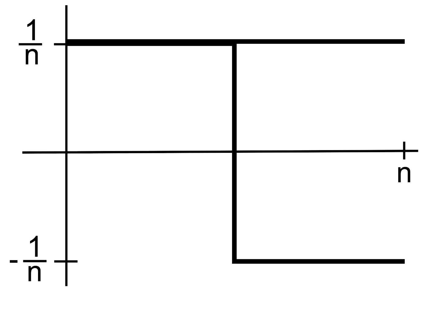
Level 0: $\psi_{1},\psi_{2}$

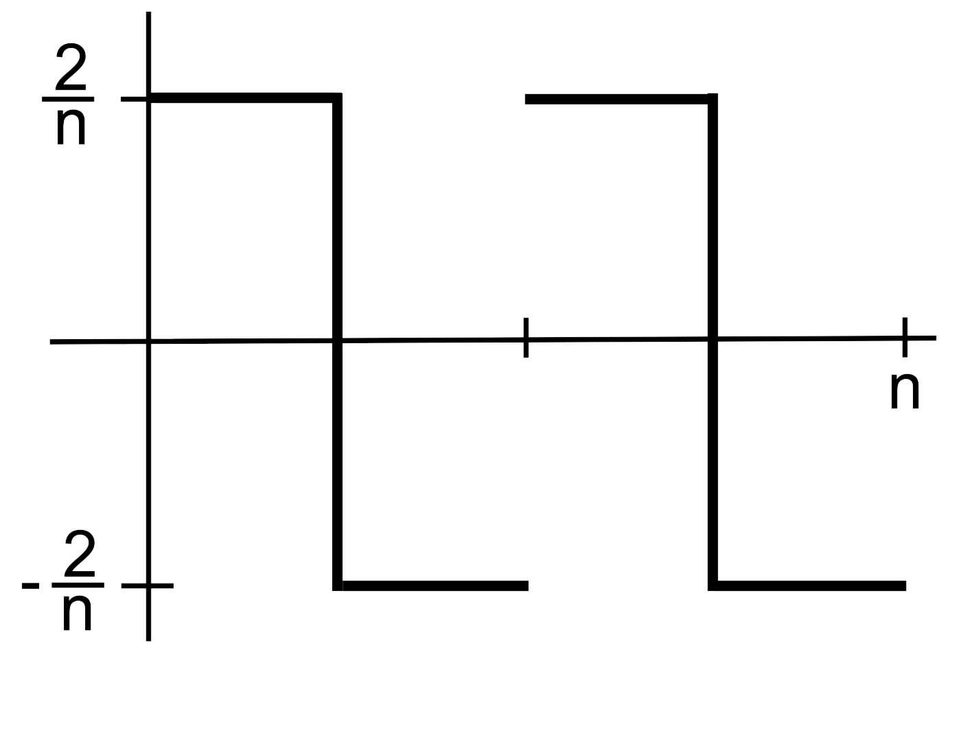
Level 1: $\psi_{3},\psi_{4}$

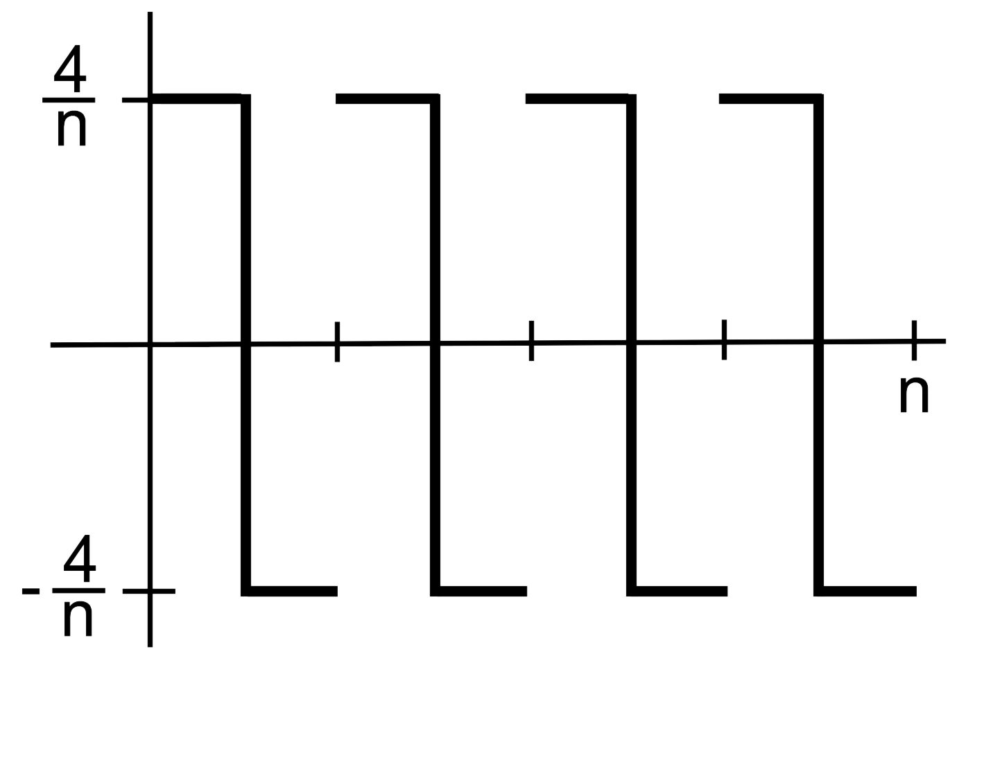
Level 2: $\psi_{5},\dots,\psi_{8}$

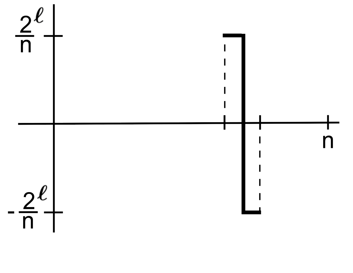
Level $\ell$

…

Figure 2. Haar basis

3.2. Formal construction

First observe that the regularity property (3.1) of a probability distribution on $\mathbb{R}^{n}$ passes on to the marginal distributions. For example, regularity of a random vector $(X_{1},X_{2})\in\mathbb{R}^{2}$ means that

$$f_{(X_{1},X_{2})}(x_{1},x_{2})\leq\exp(-\mathinner{\!\left\lvert x_{1}-y_{1}\right\rvert}-\mathinner{\!\left\lvert x_{2}-y_{2}\right\rvert})\,f_{(X_{1},X_{2})}(y_{1},y_{2}),$$

for all $(x_{1},y_{1}),(x_{2},y_{2})\in\mathbb{R}^{2}$. In particular,

$$f_{(X_{1},X_{2})}(x_{1},x_{2})\leq\exp(-\mathinner{\!\left\lvert x_{2}-y_{2}\right\rvert})\,f_{(X_{1},X_{2})}(x_{1},y_{2}).$$

Taking integral with respect to $x_{1}$ on both sides yields

$$f_{X_{2}}(x_{2})\leq\exp(-\mathinner{\!\left\lvert x_{2}-y_{2}\right\rvert})\,f_{X_{2}}(y_{2}),$$

which is equivalent to the regularity of the random vector $X_{2}\in\mathbb{R}^{1}$. The same argument works in higher dimensions.

Thus, by dropping at most $n/2$ terms if necessary, we can assume without loss of generality that

$$n=2^{L}\quad\text{for some }L\in\mathbb{N}.$$ (3.6)

Consider i.i.d. random variables $\Lambda_{1},\ldots,\Lambda_{n}\sim\operatorname{Lap}(L+2)$ and the Haar basis $\psi_{1},\ldots,\psi_{n}$ of $\ell^{2}[n]$ introduced in the previous subsection. Define the random function $Z\mathrel{\mathop{\mathchar 58\relax}}[n]\to\mathbb{R}$ by

$$Z=\sum_{j=1}^{n}\Lambda_{j}\psi_{j}.$$

Define the increments by $Z_{i}=Z(i)$ for $i=1,\ldots,n$. The construction is complete. It remains to check boundedness and regularity.

3.3. Boundedness

Fix $k\in[n]$. We would like to bound the partial sum

$$S_{k}\coloneqq\sum_{i=1}^{k}Z_{i}=\sum_{i=1}^{k}Z(i)=\langle Z,{\textbf{1}}_{[k]}\rangle=\sum_{j=1}^{n}\Lambda_{j}a_{kj}\quad\text{where}\quad a_{kj}=\langle\psi_{j},{\textbf{1}}_{[k]}\rangle.$$

(Here we use the inner product in $\ell^{2}[n]$, and denote by ${\textbf{1}}_{[k]}$ the indicator of the discrete interval $[k]=\{1,\ldots,k\}$.)

For every $k,j\in[n]$ we have

$$\mathinner{\!\left\lvert a_{kj}\right\rvert}\leq\mathinner{\!\bigl{\lVert}\psi_{j}\bigr{\rVert}}_{1}\mathinner{\!\bigl{\lVert}{\textbf{1}}_{[1,k]}\bigr{\rVert}}_{\infty}=1.$$

Moreover, the random variables $\Lambda_{j}\sim\operatorname{Lap}(L+2)$ are subexponential, and $\mathinner{\!\left\lVert\Lambda_{j}\right\rVert}_{\psi_{1}}\lesssim L$. Hence

$$\mathinner{\!\left\lVert\Lambda_{j}a_{kj}\right\rVert}_{\psi_{1}}\lesssim L\quad\forall k,j\in[n].$$ (3.7)

Furthermore, we claim that for each $k\in[n]$, at most $L+2$ terms $a_{kj}$ are nonzero. Indeed, let us fix $k$ and recall that the definition of Haar functions yields

$$a_{kj}=\langle\psi_{j},{\textbf{1}}_{[k]}\rangle=0\quad\text{if }k\not\in\operatorname{supp}(\psi_{j}).$$

On any given level $\ell\in\{1,\ldots,L\}$, the Haar functions $\psi_{j}$ have disjoint support, so there is a single $j=j(k,\ell)$ for which $k\in\operatorname{supp}(\psi_{j})$. Therefore, for each level $\ell\in\{1,\ldots,L\}$, there can be at most one nonzero coefficient $a_{kj}$. Two more nonzero coefficients can be on level $\ell=0$, coming from the functions $\phi_{1}$ and $\phi_{2}$. This proves our claim that, for each $k\in[n]$, there number of nonzero coefficients $a_{kj}$ is bounded by $L+2$.

Summarizing, we showed that for each $k\in[n]$, the sum $S_{k}=\sum_{j=1}^{n}\Lambda_{j}a_{kj}$ is a sum of at most $L+2$ independent mean zero subexponential random variables that satisfy (3.7). Applying Bernstein’s inequality (see [48, Theorem 2.8.1]), we obtain for every $k\in[n]$ and $t\geq 0$:

$$\mathbb{P}\left\{\mathinner{\!\left\lvert S_{k}\right\rvert}\geq t\rule{0.0pt}{8.53581pt}\right\}\leq 2\exp\left(-c\min(t^{2}/L^{3},\,t/L)\right).$$

Let $s\geq 1$ and apply this bound for $t=CsL^{2}$ where $C$ is a sufficiently large absolute constant. We obtain

$$\mathbb{P}\left\{\mathinner{\!\left\lvert S_{k}\right\rvert}\geq CsL^{2}\rule{0.0pt}{8.53581pt}\right\}\leq 2\exp\left(-2\min(s^{2},s)L\right)\leq\frac{2}{n}\exp(-s),$$

where we used that $s\geq 1$ and (3.6) in the last step. Taking the union bound over $k\in[n]$, we get

$$\mathbb{P}\left\{\max_{1\leq k\leq n}\mathinner{\!\left\lvert S_{k}\right\rvert}\geq CsL^{2}\rule{0.0pt}{8.53581pt}\right\}\leq 2\exp(-s)\quad\forall s\geq 1.$$

This implies that $\operatorname{\mathbb{E}}\max_{1\leq k\leq n}\mathinner{\!\left\lvert S_{k}\right\rvert}\lesssim L^{2}\lesssim\log^{2}n$ and proves the first boundedness property (3.2).

The second boundedness property (3.3) follows similarly, and even in a simpler way, if we choose $t=CsL^{3/2}$ and bypass the union bound.

3.4. Regularity

Recall that the Haar functions $\psi_{1},\ldots,\psi_{n}$ form an orthogonal basis of $\ell^{2}[n]$. However, this basis is not orthonormal, as the norm of each function $\psi_{j}$ on level $\ell$ satisfies $\mathinner{\lVert\psi_{j}\rVert}_{2}^{2}=2^{\ell}/n$. Thus, every function $x\in\ell^{2}[n]$ admits the orthogonal decomposition

$$x=\sum_{j=1}^{n}\lambda(x)_{j}\,\psi_{j}\quad\text{where }\lambda(x)_{j}=\frac{n}{2^{\ell}}\langle\psi_{j},x\rangle.$$

The key property of the coefficient vector $\lambda(x)$ is its approximate sparsity, which we can express via the $\ell^{1}$ norm.

Lemma 3.2 (Sparsity).

For any function $x\in\ell^{2}[n]$, the coefficient vector $\lambda(x)$ satisfies

$$\mathinner{\!\left\lVert\lambda(x)\right\rVert}_{1}\leq(L+2)\mathinner{\!\left\lVert x\right\rVert}_{1}.$$

Proof.

First, let us prove the lemma for the indicator of any single point $k\in[n]$, i.e. for $x={\textbf{1}}_{\{k\}}$. Here we have

$$\lambda(x)_{j}=\frac{n}{2^{\ell}}\psi_{j}(k).$$

By construction, any function $\psi_{j}$ on level $\ell$ takes on three values: $0$ and $\pm 2^{\ell}/n$. Moreover, on any given level $\ell\geq 1$, the functions $\psi_{j}$ have disjoint support, so there is a single well-defined $j=j(k,\ell)$ for which $k\in\operatorname{supp}(\psi_{j})$. Therefore, among all functions $\psi_{j}$ on a given level $\ell\geq 1$, only one can make $\lambda(x)_{j}$ nonzero, namely the one with $j=j(k,\ell)$, and such a nonzero value always equals $(n/2^{\ell})(\pm 2^{\ell}/n)=\pm 1$. Summarizing, the level $\ell=0$ contributes two nonzero coefficients $\lambda(x)_{j}$, while each further level $\ell\in\{1,\ldots,L\}$ contributes only one. Hence $\lambda(x)$ has $L+2$ nonzero coefficients $\lambda(x)_{j}$, each taking values $\pm 1$. Therefore, $\mathinner{\!\left\lVert\lambda(x)\right\rVert}_{1}\leq L+2$.

To extend this bound to a general function $x\in\ell^{2}[n]$, decompose it as $x=\sum_{k=1}^{n}x(k){\textbf{1}}_{\{k\}}$. Then, by linearity, $\lambda(x)=\sum_{k=1}^{n}x(k)\lambda({\textbf{1}}_{\{k\}})$, so

$$\mathinner{\!\left\lVert\lambda(x)\right\rVert}_{1}\leq\sum_{k=1}^{n}\mathinner{\!\left\lvert x(k)\right\rvert}\,\mathinner{\!\bigl{\lVert}\lambda({\textbf{1}}_{\{k\}})\bigr{\rVert}}_{1}.$$

The bound $\mathinner{\!\bigl{\lVert}\lambda({\textbf{1}}_{\{k\}})\bigr{\rVert}}_{1}\leq L+2$ from the first part of the argument completes the proof of the lemma. ∎

We are ready to prove regularity. Consider the random function $Z=\sum_{j=1}^{n}\Lambda_{j}\psi_{j}$ constructed in Subsection 3.2. In our new notation, the coefficient vector of $Z$ is $\lambda(Z)=(\Lambda_{1},\ldots,\Lambda_{n})=\mathrel{\mathop{\mathchar 58\relax}}\Lambda$. We have for any $x,y\in\ell^{2}[n]$:

$$r(x,y)\coloneqq\frac{\operatorname{dens}_{X}(x)}{\operatorname{dens}_{X}(y)}=\frac{\operatorname{dens}_{\Lambda}(\lambda(x))}{\operatorname{dens}_{\Lambda}(\lambda(y))}.$$ (3.8)

To see this, recall that the map $x\mapsto\lambda(x)$ is a linear bijection on $\ell^{2}[n]$. Hence for any $\varepsilon>0$ and for the unit ball $B$ of $\ell^{2}[n]$, we have

$$\frac{\mathbb{P}\left\{X\in x+\varepsilon B\rule{0.0pt}{8.53581pt}\right\}}{\mathbb{P}\left\{X\in y+\varepsilon B\rule{0.0pt}{8.53581pt}\right\}}=\frac{\mathbb{P}\left\{\Lambda\in\lambda(x)+\varepsilon\lambda(B)\rule{0.0pt}{8.53581pt}\right\}}{\mathbb{P}\left\{\Lambda\in\lambda(y)+\varepsilon\lambda(B)\rule{0.0pt}{8.53581pt}\right\}}.$$

Taking the limit on both sides as $\varepsilon\to 0_{+}$ and applying the Lebesgue differentiation theorem yield (3.8).

By construction, the coefficients $\Lambda_{i}$ of the random vector $\Lambda\in\mathbb{R}^{n}$ are $\operatorname{Lap}(L+2)$ i.i.d. random variables. Hence

$$\operatorname{dens}_{\Lambda}(z)=\frac{1}{2(L+2)}\exp\Big{(}-\frac{\mathinner{\!\left\lVert z\right\rVert}_{1}}{L+2}\Big{)},\quad z\in\mathbb{R}^{n}.$$

Thus,

$$r(x,y)=\exp\Bigg{(}\frac{\mathinner{\!\left\lVert\lambda(y)\right\rVert}_{1}-\mathinner{\!\left\lVert\lambda(x)\right\rVert}_{1}}{L+2}\Bigg{)}.$$

By the triangle inequality and Lemma 3.2, we have

$$\mathinner{\!\left\lVert\lambda(y)\right\rVert}_{1}-\mathinner{\!\left\lVert\lambda(x)\right\rVert}_{1}\leq\mathinner{\!\left\lVert\lambda(x)-\lambda(y)\right\rVert}_{1}\leq(L+2)\mathinner{\!\left\lVert x-y\right\rVert}_{1}.$$

Thus

$$r(x,y)\leq\exp(\mathinner{\!\left\lVert x-y\right\rVert}_{1}).$$

If we express the density in the form $\operatorname{dens}_{X}(x)=\frac{1}{\beta}e^{-V}$, the bound we proved can be written as

$$\exp\left(V(y)-V(x)\right)\leq\exp(\mathinner{\!\left\lVert x-y\right\rVert}_{1}),$$

or $V(y)-V(x)\leq\mathinner{\!\left\lVert x-y\right\rVert}_{1}$. Swapping $x$ with $y$ yields $\mathinner{\!\left\lvert V(x)-V(y)\right\rvert}\leq\mathinner{\!\left\lVert x-y\right\rVert}_{1}$. The proof of Theorem 3.1 is complete. ∎

3.5. Optimality

The reader might wonder if the logarithmic factors are necessary in Theorem 3.1. While we do not know if this is the case for the bound (3.3), the logarithmic factor can not be completely removed from the uniform bound (3.2):

Proposition 3.3 (Logarithm is needed in (3.2)).

Let $n\geq 4$ be a natural number and consider a probability density of the form $f(z)=\frac{1}{\beta}e^{-V(z)}$ on $\mathbb{R}^{n}$. Assume that the potential $V$ is $1$-Lipschitz in the $\ell^{1}$-norm, i.e. (3.1) holds. Then a random vector $Z=(Z_{1},\ldots,Z_{n})$ distributed according to the density $f$ satisfies

$$\operatorname{\mathbb{E}}\max_{1\leq k\leq n}\mathinner{\!\left\lvert Z_{1}+\cdots+Z_{k}\right\rvert}\geq\frac{1}{8}\log n.$$

Proof.

Since triangle inequality yields $\mathinner{\!\left\lVert Z\right\rVert}_{\infty}=\max_{1\leq k\leq n}\mathinner{\!\left\lvert Z_{k}\right\rvert}\leq 2\max_{1\leq k\leq n}\mathinner{\!\left\lvert Z_{1}+\cdots+Z_{k}\right\rvert}$, it suffices to check that

$$\operatorname{\mathbb{E}}\mathinner{\!\left\lVert Z\right\rVert}_{\infty}\geq\frac{1}{4}\log n.$$

Assume for contradiction that this bound fails. Then, considering the cube

$$Q=\left\{z\in\mathbb{R}^{n}\mathrel{\mathop{\mathchar 58\relax}}\;\mathinner{\!\left\lVert z\right\rVert}_{\infty}<\frac{1}{2}\log n\right\},$$

we obtain by Markov’s inequality that $\mathbb{P}\left\{Z\in Q\rule{0.0pt}{8.53581pt}\right\}>1/2$.

Let $e_{1},\ldots,e_{n}$ denote the standard basis vectors in $\mathbb{R}^{n}$ and consider the following translates of the cube $Q$:

$$Q_{i}=Q+\frac{1}{2}\log(n)\,e_{i},\quad i=1,\ldots,n.$$

Note the following two properties. First, the cubes $Q_{i}$ are disjoint. Second, since $V$ is $1$-Lipschitz in the $\ell^{1}$-norm, for each $i=1,\ldots,n$, the densities of the random vectors $Z$ and $Z-\frac{1}{2}\log(n)\,e_{i}$ and $(Z_{1},\ldots,Z_{n})$ differ by a multiplicative factor of at most $\exp(\frac{1}{2}\log n)=\sqrt{n}$ pointwise. Therefore,

$$\mathbb{P}\left\{Z\in Q_{i}\rule{0.0pt}{8.53581pt}\right\}=\mathbb{P}\left\{Z-\frac{1}{2}\log(n)\,e_{i}\in Q\rule{0.0pt}{8.53581pt}\right\}\geq\frac{1}{\sqrt{n}}\mathbb{P}\left\{Z\in Q\rule{0.0pt}{8.53581pt}\right\}>\frac{1}{2\sqrt{n}},\quad i=1,\ldots,n.$$

Hence, using these two properties we get

$$1\geq\sum_{i=1}^{n}\mathbb{P}\left\{Z\in Q_{i}\rule{0.0pt}{8.53581pt}\right\}>\frac{\sqrt{n}}{2}.$$

It follows that $n<4$, which contradicts the assumption of the lemma. The proof is complete. ∎

3.6. Beyond the $\ell^{1}$ norm?

One may wonder why specifically the $\ell^{1}$ norm appears in the regularity property of Theorem 3.1. As we will see shortly, the regularity with respect to the $\ell^{1}$ norm is exactly what is needed in our applications to privacy. However, it might be interesting to see if there are natural extensions of Theorem 3.1 for general $\ell^{p}$ norms. The lemma below rules out one such avenue, showing that if a potential $V$ is Lipschitz with respect to the $\ell^{p}$ norm for some $p>1$, the corresponding random walk deviates at least polynomially fast (as opposed to logarithmically fast).

Proposition 3.4 (No boundedness for $\ell^{p}$-regular potentials).

Let $n\in\mathbb{N}$ and consider a probability density of the form $f(z)=\frac{1}{\beta}e^{-V(z)}$ on $\mathbb{R}^{n}$. Assume that the potential $V$ is $1$-Lipschitz in the $\ell^{p}$-norm. Then a random vector $Z=(Z_{1},\ldots,Z_{n})$ distributed according to the density $f$ satisfies

$$\operatorname{\mathbb{E}}\mathinner{\!\left\lvert Z_{1}+\cdots+Z_{n}\right\rvert}\geq\frac{1}{4}n^{1-\frac{1}{p}}.$$

Proof.

We can write $Z_{1}+\cdots+Z_{n}=\langle Z,u\rangle$ where $u=(1,\ldots,1)^{\mathsf{T}}$. Since $\mathinner{\lVert n^{-\frac{1}{p}}u\rVert}_{p}=1$ and $V$ is 1-Lipschitz in the $\ell^{p}$ norm, the densities of the random vectors $Z+n^{-\frac{1}{p}}u$ and $Z$ differ by a multiplicative factor of at most $e$ pointwise. Therefore,

$$\operatorname{\mathbb{E}}\mathinner{\!\left\lvert\langle Z,u\rangle\right\rvert} \geq e^{-1}\operatorname{\mathbb{E}}\mathinner{\!\bigl{\lvert}\langle Z+n^{-\frac{1}{p}}u,u\rangle\bigr{\rvert}}$$

$$\geq e^{-1}\Big{(}\mathinner{\!\bigl{\lvert}\langle n^{-\frac{1}{p}}u,u\rangle\bigr{\rvert}}-\operatorname{\mathbb{E}}\mathinner{\!\left\lvert\langle Z,u\rangle\right\rvert}\Big{)}\quad\text{(by triangle inequality)}$$

$$=e^{-1}\Big{(}n^{1-\frac{1}{p}}-\operatorname{\mathbb{E}}\mathinner{\!\left\lvert\langle Z,u\rangle\right\rvert}\Big{)}.$$

Rearranging the terms, we deduce that

$$\operatorname{\mathbb{E}}\mathinner{\!\left\lvert\langle Z,u\rangle\right\rvert}\geq\frac{e^{-1}}{1+e^{-1}}n^{1-\frac{1}{p}}\geq\frac{1}{4}n^{1-\frac{1}{p}},$$

which completes the proof. ∎

In light of Theorem 3.1 and Proposition 3.4 it might be interesting to see if an obstacle remains for the density $f(z)=\frac{1}{\beta}e^{-V(z)^{p}}$ for $p>1$.

4. Metric privacy

4.1. Private measures

The superregular random walk we just constructed will become the main tool in solving the following private measure problem. We are looking for a private and accurate algorithm $\mathcal{A}$ that transforms a probability measure $\mu$ on a metric space $(T,\rho)$ into another finitely-supported probability measure $\mathcal{A}(\mu)$ on $(T,\rho)$.

We need to specify what we mean by privacy and accuracy here. Metric privacy offers a natural framework for our problem. Namely, we consider Definition 2.2 for the space $(\mathcal{M}(T),\mathrm{TV})$ of all probability measures on $T$ equipped with the TV metric (recalled in Section 2.2.1). Thus, for any pair of input measures $\mu$ and $\mu^{\prime}$ on $T$ that are close in the TV metric, we would like the distributions of the (random) output measures $\mathcal{A}(\mu)$ and $\mathcal{A}(\mu^{\prime})$ to be close:

$$\frac{\mathbb{P}\left\{\mathcal{A}(\mu)\in S\rule{0.0pt}{8.53581pt}\right\}}{\mathbb{P}\left\{\mathcal{A}(\mu^{\prime})\in S\rule{0.0pt}{8.53581pt}\right\}}\leq\exp\left(\alpha\mathinner{\lVert\mu-\mu^{\prime}\rVert}_{\mathrm{TV}}\right).$$ (4.1)

The accuracy will be measured via the Wasserstein distance (recalled in Section 2.2.2). We hope to make $W_{1}(\mathcal{A}(\mu),\mu)$ as small as possible. The reason for choosing $W_{1}$ as distance is that it allows us to derive accuracy guarantees for general Lipschitz statistics, as outlined below.

4.2. Synthetic data

The private measure problem has an immediate application for differentially private synthetic data. Let $(T,\rho)$ be a compact metric space. We hope to find an algorithm $\mathcal{B}$ that transforms the true data $X=(X_{1},\ldots,X_{n})\in T^{n}$ into synthetic data $Y=(Y_{1},\ldots,Y_{m})\in T^{m}$ for some $m$ such that the empirical measures

$$\mu_{X}=\frac{1}{n}\sum_{i=1}^{n}\delta_{X_{i}}\quad\text{and}\quad\mu_{Y}=\frac{1}{m}\sum_{i=1}^{m}\delta_{Y_{i}}$$

are close in the Wasserstein distance, i.e. we hope to make $W_{1}(\mu_{X},\mu_{Y})$ small. This would imply that synthetic data accurately preserves all Lipschitz statistics, i.e.

$$\frac{1}{n}\sum_{i=1}^{n}f(X_{i})\approx\frac{1}{m}\sum_{i=1}^{m}f(Y_{i})$$

for any Lipschitz function $f\mathrel{\mathop{\mathchar 58\relax}}T\to\mathbb{R}$.

This goal can be immediately achieved if we solve a version of the private measure problem, described in Section 4.1, with the additional requirement that $\mathcal{A}(\mu)$ be an empirical measure. Indeed, define the algorithm $\mathcal{B}$ by feeding the empirical measure $\mu_{X}$ into $\mathcal{A}$, i.e. set $\mathcal{B}(X)=\mathcal{A}(\mu_{X})$. The accuracy follows, and the differential privacy of $\mathcal{B}$ can be seen as follows.

For any pair $X,X^{\prime}$ of input data that differ in a single element, the corresponding empirical measures differ by at most $1/n$ with respect to the TV distance, i.e.

$$\mathinner{\!\left\lVert\mu_{X}-\mu_{X^{\prime}}\right\rVert}_{\mathrm{TV}}\leq\frac{1}{n}.$$

Then, for any subset $S$ in the output space, we can use (4.1) to get

$$\frac{\mathbb{P}\left\{\mathcal{B}(X)\in S\rule{0.0pt}{8.53581pt}\right\}}{\mathbb{P}\left\{\mathcal{B}(X^{\prime})\in S\rule{0.0pt}{8.53581pt}\right\}}=\frac{\mathbb{P}\left\{\mathcal{A}(\mu_{X})\in S\rule{0.0pt}{8.53581pt}\right\}}{\mathbb{P}\left\{\mathcal{A}(\mu_{X^{\prime}})\in S\rule{0.0pt}{8.53581pt}\right\}}\leq\exp\left(\alpha\,\mathinner{\lVert\mu-\mu^{\prime}\rVert}_{\mathrm{TV}}\right)\leq\exp(\alpha/n).$$

Thus, if $\alpha=\varepsilon n$, the algorithm $\mathcal{B}$ is $\varepsilon$-differentially private. Let us record this observation formally.

Lemma 4.1 (Private measure yields private synthetic data).

Let $(T,\rho)$ be a compact metric space. Let $\mathcal{A}$ be an algorithm that inputs a probability measure on $T$, and outputs something. Define the algorithm $\mathcal{B}$ that takes data $X=(X_{1},\ldots,X_{n})\in T^{n}$ as an input, creates the empirical measure $\mu_{X}$ and feeds it into the algorithm $\mathcal{A}$, i.e. set $\mathcal{B}(X)=\mathcal{A}(\mu_{X})$. If $\mathcal{A}$ is $\alpha$-metrically private in the TV metric and $\alpha=\varepsilon n$, then $\mathcal{B}$ is $\varepsilon$-differentially private.

Thus, our main focus from now on will be on solving the private measure problem; private synthetic data will follows as a consequence.

5. A private measure on the line

In this section, we construct a private measure on the interval $[0,1]$. Later we will extend this construction to general metric spaces.

5.1. Discrete input space

Let us start with a somewhat restricted goal, and then work toward wider generality. In this subsection, we will (a) assume that the input measure $\mu$ is always supported on some fixed finite subset

$$\Omega=\{\omega_{1},\ldots,\omega_{n}\}\quad\text{where }0\leq\omega_{1}\leq\cdots\leq\omega_{n}\leq 1$$

and (b) allow the output $\mathcal{A}(\mu)$ to be a signed measure. We will measure accuracy with the Wasserstein distance.

5.1.1. Perturbing a measure by a superregular random walk

Apply the Superregular Random Walk Theorem 3.1 and rescale the random variables $Z_{i}$ by setting $U_{i}=(2/\alpha)Z_{i}$. The regularity property of the random vector $U=(U_{1},\ldots,U_{n})$ takes the form

$$\frac{\operatorname{dens}_{Y}(x)}{\operatorname{dens}_{Y}(y)}\leq\exp\left(\frac{\alpha}{2}\mathinner{\!\left\lVert x-y\right\rVert}_{1}\right)\quad\text{for all }x,y\in\mathbb{R}^{n},$$ (5.1)

and the boundedness property takes the form

$$\max_{1\leq k\leq n}\operatorname{\mathbb{E}}\mathinner{\!\left\lvert U_{1}+\cdots+U_{k}\right\rvert}\leq\frac{C\log^{\frac{3}{2}}n}{\alpha}.$$ (5.2)

Let us make the algorithm $\mathcal{A}$ perturb the measure $\mu$ on $\Omega$ by the weights $U_{i}$, i.e. we set

$$\mathcal{A}(\mu)(\omega_{i})=\mu(\{\omega_{i}\})+U_{i},\quad i=1,\ldots,n.$$ (5.3)

5.1.2. Privacy

Any measure $\nu$ on $\Omega$ can be identified with the vector $\bar{\nu}\in\mathbb{R}^{n}$ by setting $\bar{\nu}_{i}=\nu(\{\omega_{i}\})$. Then, for any measure $\eta$ on $\Omega$, we have

$$\operatorname{dens}_{\mathcal{A}(\mu)}(\eta)=\operatorname{dens}_{\bar{\mu}+Y}(\bar{\eta})=\operatorname{dens}_{Y}(\bar{\eta}-\bar{\mu}).$$ (5.4)

Fix two measures $\mu$ and $\mu^{\prime}$ on $\Omega$. By above, we have

$$\frac{\operatorname{dens}_{\mathcal{A}(\mu)}(\eta)}{\operatorname{dens}_{\mathcal{A}(\mu^{\prime})}(\eta)} =\frac{\operatorname{dens}_{Y}(\bar{\eta}-\bar{\mu})}{\operatorname{dens}_{Y}(\bar{\eta}-\bar{\mu^{\prime}})}\quad\text{(by \eqref{eq: measure to vector})}$$

$$\leq\exp\left(\frac{\alpha}{2}\mathinner{\!\left\lVert\bar{\mu}-\bar{\mu^{\prime}}\right\rVert}_{1}\right)\quad\text{(by \eqref{eq: Y regularity})}$$

$$=\exp\left(\alpha\mathinner{\!\left\lVert\mu-\mu^{\prime}\right\rVert}_{\mathrm{TV}}\right)\quad\text{(by \eqref{eq: TV as L1})}.$$

This shows that the algorithm $\mathcal{A}$ is $\alpha$-metrically private in the TV metric.

5.1.3. Accuracy

If $\nu$ and $\mu$ are signed measures on $\Omega$, then with the definition (2.7) of the Wasserstein metric for signed measures, we have

$$W_{1}(\nu,\mu) =\int_{0}^{1}|\nu([0,x])-\mu([0,x])|\,dx$$

$$=\int_{0}^{1}\left|\sum_{i\mathrel{\mathop{\mathchar 58\relax}}\;\omega_{i}\leq x}(\nu(\{\omega_{i}\})-\sum_{i\mathrel{\mathop{\mathchar 58\relax}}\;\omega_{i}\leq x}\mu(\{\omega_{i}\})\right|\,dx$$

$$=\sum_{k=1}^{n}(\omega_{k+1}-\omega_{k})\left|\sum_{i=1}^{k}\nu(\{\omega_{i}\})-\sum_{i=1}^{k}\mu(\{\omega_{i}\})\right|,$$

where we set $\omega_{n+1}=1$.

Applying this general observation for $\nu=\mathcal{A}(\mu)$ and using (5.3), we obtain

$$W_{1}(\mathcal{A}(\mu),\mu)=\sum_{k=1}^{n}(\omega_{k+1}-\omega_{k})\mathinner{\!\left\lvert U_{1}+\cdots+U_{k}\right\rvert}.$$

Take expectation on both sides and use (5.2) to conclude that

$$\operatorname{\mathbb{E}}W_{1}(\mathcal{A}(\mu),\mu)\leq\frac{C\log^{\frac{3}{2}}n}{\alpha}.$$

The following result summarizes what we have proved.

Proposition 5.1 (Input in discrete space, output signed measure).

Let $\Omega$ be finite subset of $[0,1]$ and let $n=\mathinner{\!\left\lvert\Omega\right\rvert}$. Let $\alpha>0$. There exists a randomized algorithm $\mathcal{A}$ that takes a probability measure $\mu$ on $\Omega$ as an input and returns a signed measure $\nu$ on $\Omega$ as an output, and with the following two properties.

1. (Privacy): the algorithm $\mathcal{A}$ is $\alpha$-metrically private in the TV metric.

2. (Accuracy): for any input measure $\mu$, the expected accuracy of the output signed measure $\nu$ in the Wasserstein distance is

   $$\operatorname{\mathbb{E}}W_{1}(\nu,\mu)\leq\frac{C\log^{\frac{3}{2}}n}{\alpha}.$$

Let $\nu$ be the signed measure obtained in Proposition 5.1. Let $\widehat{\nu}$ be a probability measure on $\Omega$ that minimizes $W_{1}(\widehat{\nu},\nu)$. (The minimizer could be non-unique.) Note that this is a convex problem, since by (LABEL:wassersteinformula), this problem is equivalent to minimizing

$$\sum_{k=1}^{n}(\omega_{k+1}-\omega_{k})\left|\sum_{i=1}^{k}\widehat{\nu}(\{\omega_{i}\})-\sum_{i=1}^{k}\nu(\{\omega_{i}\})\right|,$$

under the constraints $\widehat{\nu}(\{\omega_{i}\})\geq 0$ and $\sum_{i=1}^{k}\widehat{\nu}(\{\omega_{i}\})=1$.

By minimality, $W_{1}(\widehat{\nu},\nu)\leq W_{1}(\mu,\nu)$. So $W_{1}(\widehat{\nu},\mu)\leq W_{1}(\widehat{\nu},\nu)+W_{1}(\nu,\mu)\leq 2W_{1}(\mu,\nu)$.

Proposition 5.2 (Private measure on a finite subset of the interval).

Let $\Omega$ be finite subset of $[0,1]$ and let $n=\mathinner{\!\left\lvert\Omega\right\rvert}$. Let $\alpha>0$. There exists a randomized algorithm $\mathcal{B}$ that takes a probability measure $\mu$ on $\Omega$ as an input and returns a probability measure $\nu$ on $\Omega$ as an output, and with the following two properties.

1. (Privacy): the algorithm $\mathcal{B}$ is $\alpha$-metrically private in the TV metric.

2. (Accuracy): for any input measure $\mu$, the expected accuracy of the output measure $\nu$ in the Wasserstein distance is

   $$\operatorname{\mathbb{E}}W_{1}(\nu,\mu)\leq\frac{C\log^{\frac{3}{2}}n}{\alpha}.$$

5.2. Extending the input space to the interval

Next, we would like to extend our framework to a continuous setting, and allow measures to be supported by the entire interval $[0,1]$. We can do this by quantization.

5.2.1. Quantization

Fix $n\in\mathcal{N}$ and let $\mathcal{N}=\{\omega_{1},\ldots,\omega_{n}\}$ be a $(1/n)$-net of $[0,1]$. Consider the proximity partition

$$[0,1]=I_{1}\cup\cdots\cup I_{n}$$

where we put a point $x\in[0,1]$ into $I_{i}$ if $x$ is closer to $\omega_{i}$ that to any other points in $\mathcal{N}$. (We break any ties arbitrarily.)

We can quantize any signed measure $\nu$ on $[0,1]$ by defining

$$\nu_{\mathcal{N}}\left(\{\omega_{i}\}\right)=\nu(I_{i}),\quad i=1,\ldots,n.$$ (5.5)

Obviously, $\nu_{\mathcal{N}}$ is a signed measure on $\mathcal{N}$. Moreover, if $\nu$ is a measure, then so is $\nu_{\mathcal{N}}$. And if $\nu$ is a probability measure, then so is $\nu_{\mathcal{N}}$. In the latter case, it follows from the construction that

$$W_{1}(\nu,\nu_{\mathcal{N}})\leq 1/n.$$ (5.6)

(By definition of the net, transporting any point $x$ to the closest point $\omega_{i}$ covers distance at most $1/n$.)

Lemma 5.3 (Quantization is a contraction in TV metric).

Any signed measure $\nu$ on $[0,1]$ satisfies

$$\mathinner{\!\left\lVert\nu_{\mathcal{N}}\right\rVert}_{\mathrm{TV}}\leq\mathinner{\!\left\lVert\nu\right\rVert}_{\mathrm{TV}}.$$

Proof.

Using (2.5), (5.5), and (2.4), we obtain

$$\mathinner{\!\left\lVert\nu_{\mathcal{N}}\right\rVert}_{\mathrm{TV}}=\frac{1}{2}\sum_{i=1}^{n}\mathinner{\!\left\lvert\nu_{\mathcal{N}}(\{\omega_{i}\})\right\rvert}=\frac{1}{2}\sum_{i=1}^{n}\mathinner{\!\left\lvert\nu(I_{i})\right\rvert}\leq\mathinner{\!\left\lVert\nu\right\rVert}_{\mathrm{TV}}.$$

The lemma is proved. ∎

5.2.2. A private measure on the interval

Theorem 5.4 (Private measure on the interval).

Let $\alpha\geq 2$. There exists a randomized algorithm $\mathcal{A}$ that takes a probability measure $\mu$ on $[0,1]$ as an input and returns a finitely-supported probability measure $\nu$ on $[0,1]$ as an output, and with the following two properties.

1. (Privacy): the algorithm $\mathcal{A}$ is $\alpha$-metrically private in the TV metric.

2. (Accuracy): for any input measure $\mu$, the expected accuracy of the output measure $\nu$ in the Wasserstein distance is

   $$\operatorname{\mathbb{E}}W_{1}\left(\nu,\mu\right)\leq\frac{C\log^{\frac{3}{2}}\alpha}{\alpha}.$$

Proof.

Take a measure $\mu$ on $[0,1]$, preprocess it by quantizing as in the previous subsection, and feed the quantized measure $\mu_{\mathcal{N}}$ into the algorithm $\mathcal{B}$ of Proposition 5.2 for $\Omega=\mathcal{N}$.

The contraction property (Lemma 5.3) ensures that

$$\mathinner{\!\left\lVert\mu_{\mathcal{N}}-\mu^{\prime}_{\mathcal{N}}\right\rVert}_{\mathrm{TV}}\leq\mathinner{\!\left\lVert\mu-\mu^{\prime}\right\rVert}_{\mathrm{TV}}.$$

This and the privacy property of Proposition 5.2 for measures on $\mathcal{N}$ guarantee that quantization does not destroy privacy, i.e. the algorithm $\mu\mapsto\mathcal{B}(\mu_{\mathcal{N}})$ is still $\alpha$-metrically private as claimed.

As for the accuracy, Proposition 5.2 for the measure $\mu_{\mathcal{N}}$ gives

$$\operatorname{\mathbb{E}}W_{1}\left(\mathcal{B}(\mu_{\mathcal{N}}),\mu_{\mathcal{N}}\right)\leq\frac{C\log^{\frac{3}{2}}n}{\alpha}.$$

Moreover, the accuracy of quantization (5.6) states that $W_{1}(\mu,\mu_{\mathcal{N}})\leq 1/n$. By triangle inequality, we conclude that

$$\operatorname{\mathbb{E}}W_{1}\left(\mathcal{B}(\mu_{\mathcal{N}}),\mu\right)\leq\frac{1}{n}+\frac{C\log^{\frac{3}{2}}n}{\alpha}.$$

Taking $n$ to be the largest integer less than or equal to $\alpha$ yields the conclusion of the theorem. ∎

6. The Traveling Salesman Problem

In order to extend the construction of the private measure on the interval $[0,1]$ to a general metric space $(T,\rho)$, a natural approach would be to map the interval $[0,1]$ onto some space-filling curve of $T$. Since a space filling curves usually are infinitely long, we should do this on the discrete level, for some $\delta$-net of $T$ rather than $T$ itself. In this section, we will bound length of such discrete space-filling curve in terms of the metric geometry of $T$. In the next section, we will see how this bound determines the accuracy of a private measure in $T$.

A natural framework for this step is related to Traveling Salesman Problem (TSP), which is a central problem in optimization and computer science, and whose history goes back to at least 1832 [6].

Let $G=(V,E)$ be an undirected weighted connected graph. We occasionally refer to the weights of the edges as lengths. A tour of $G$ is a connected walk on the edges that visits every vertex at least once, and returns to the starting vertex. The TSP is the problem of finding a tour of $G$ with the shortest length. Let us denote this length by $\operatorname{TSP}(G)$.

Although it is NP-hard to compute TSP(G), or even to approximate it within a factor of $123/122$ [30], an algorithm of Christofides and Serdyukov [16, 43] from 1976 gives a $3/2$-approximation for TSP, and it was shown recently that the factor $3/2$ can be further improved [29].

6.1. TSP in terms of the minimum spanning tree

Within a factor of $2$, the traveling salesman problem is equivalent to another key problem, namely the problem of finding the minimum spanning tree (MST) of $G$. A spanning tree of $G$ is a subgraph that is a tree and which includes all vertices of $G$. It always exists and can be found in polynomial time [33, 39]. A spanning tree of $G$ with the smallest length is called the minimum spanning tree of $G$; we denote its length by $\operatorname{MST}(G)$. The following equivalence is a folklore.

Lemma 6.1.

Any undirected weighted connected graph $G$ satisfies

$$\operatorname{MST}(G)\leq\operatorname{TSP}(G)\leq 2\operatorname{MST}(G).$$

Proof.

For the lower bound, it is enough to find a spanning tree of $G$ of length bounded by $\operatorname{TSP}(G)$. Consider the minimal tour of $G$ of length $\operatorname{TSP}(G)$ as a subgraph of $G$. Let $T$ be a spanning tree of the tour. Since the tour contains all vertices of $G$, so does $T$, and thus $T$ is a spanning tree of $G$. Since $T$ is obtained by removing some edges of the tour, the length of $T$ is bounded by of the tour, which is $\operatorname{TSP}(G)$. The lower bound is proved.

For the upper bound, note that dropping any edges of $G$ can only increase the value of TSP. Thus TSP of $G$ is bounded by the TSP of its spanning tree $T$. Moreover, TSP of any tree $T$ equals twice the sum of lengths of the edges of $T$. This can be seen by considering the depth-first search tour of $T$, which starts at the root and explores as deep as possible along each branch before backtracking, see Figure 3. ∎

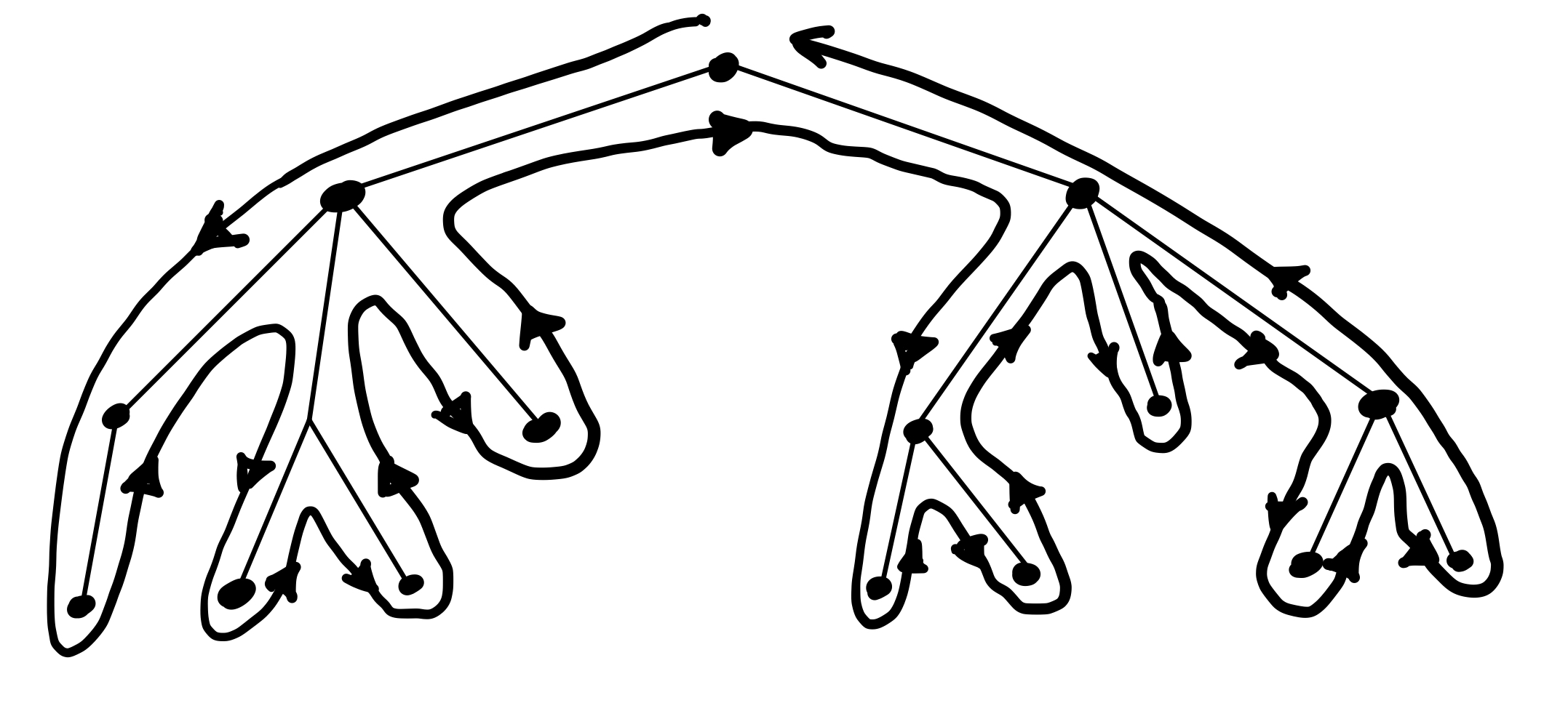
Figure 3. The depth-first search tour demonstrates that the TSP of a tree equals twice the sum of lengths of its edges.

6.2. Metric TSP

Let $(T,\rho)$ be a finite metric space. We can consider $T$ as a complete weighted graph, whose weights of edges are defined as the distances between the points. The TSP for $(T,\rho)$ is known as metric TSP.

Although a tour can visit the same vertex of $T$ multiple times, this can be prevented by skipping the vertices previously visited. The triangle inequality shows that skipping can only decrease the length of the tour. Therefore, the shortest tour in a complete graph is always a Hamiltonian cycle, a walk that visits all vertices of $T$ exactly once before returning to the starting vertex. Let us record this observation:

Lemma 6.2.

The TSP of a finite metric space $(T,\rho)$ equals the smallest length of a Hamiltonian cycle of $T$.

6.3. A geometric bound on TSP

We would like to compute $\operatorname{TSP}(T)$ in terms of the geometry of the metric space $(T,\rho)$. Here we will prove an upper bound on $\operatorname{TSP}(T)$ in terms of the covering numbers. Recall that the covering number $N(T,\rho,\varepsilon)$ is defined as the smallest cardinality of an $\varepsilon$-net of $T$, or equivalently the smallest number of closed balls with centers in $T$ and radii $\varepsilon$ whose union covers $T$, see [48, Section 4.2].

Theorem 6.3 (TSP via covering numbers).

For any finite metric space $(T,\rho)$, we have

$$\operatorname{TSP}(T)\leq 16\int_{0}^{\infty}\left(N(T,\rho,x)-1\right)\,dx.$$

Proof.

Step 1: constructing a spanning tree. Let us construct a small spanning tree $T_{0}$ of $T$ and use Lemma 6.1. Let $\varepsilon_{j}=2^{-j}$, $j\in\mathbb{Z}$, and let $\mathcal{N}_{j}$ be $\varepsilon_{j}$-nets of $T$ with cardinalities $\mathinner{\!\left\lvert\mathcal{N}_{j}\right\rvert}=N(T,\rho,\varepsilon_{j})$. Since $T$ is finite, we must have $\mathinner{\!\left\lvert\mathcal{N}_{j}\right\rvert}=1$ for all sufficiently small $j$. Let $j_{0}$ be the largest integer for which $\mathinner{\!\left\lvert\mathcal{N}_{j_{0}}\right\rvert}=1$.

At the root of $T_{0}$, let us put a single point that forms the net $\mathcal{N}_{j_{0}}$. At the next level, put all the points of the net $\mathcal{N}_{j_{0}+1}$, and connect them to the root by edges. The weights of these edges, which are defined as the distances of the points to the root, are all bounded by $\varepsilon_{j_{0}}$. At the next level, put all points of the net $\mathcal{N}_{j_{0}+2}$, and connect each such point to the closest point in the previous level $\mathcal{N}_{j_{0}+1}$. (Break any ties arbitrarily.) Since the latter set is a $\varepsilon_{j_{0}+1}$-net, the weights of all these edges are bounded by $\varepsilon_{j_{0}+1}$. Repeat these steps until the levels do not grow anymore, i.e. until the level contains all the points in $T$; see Figure 4 for illustration.

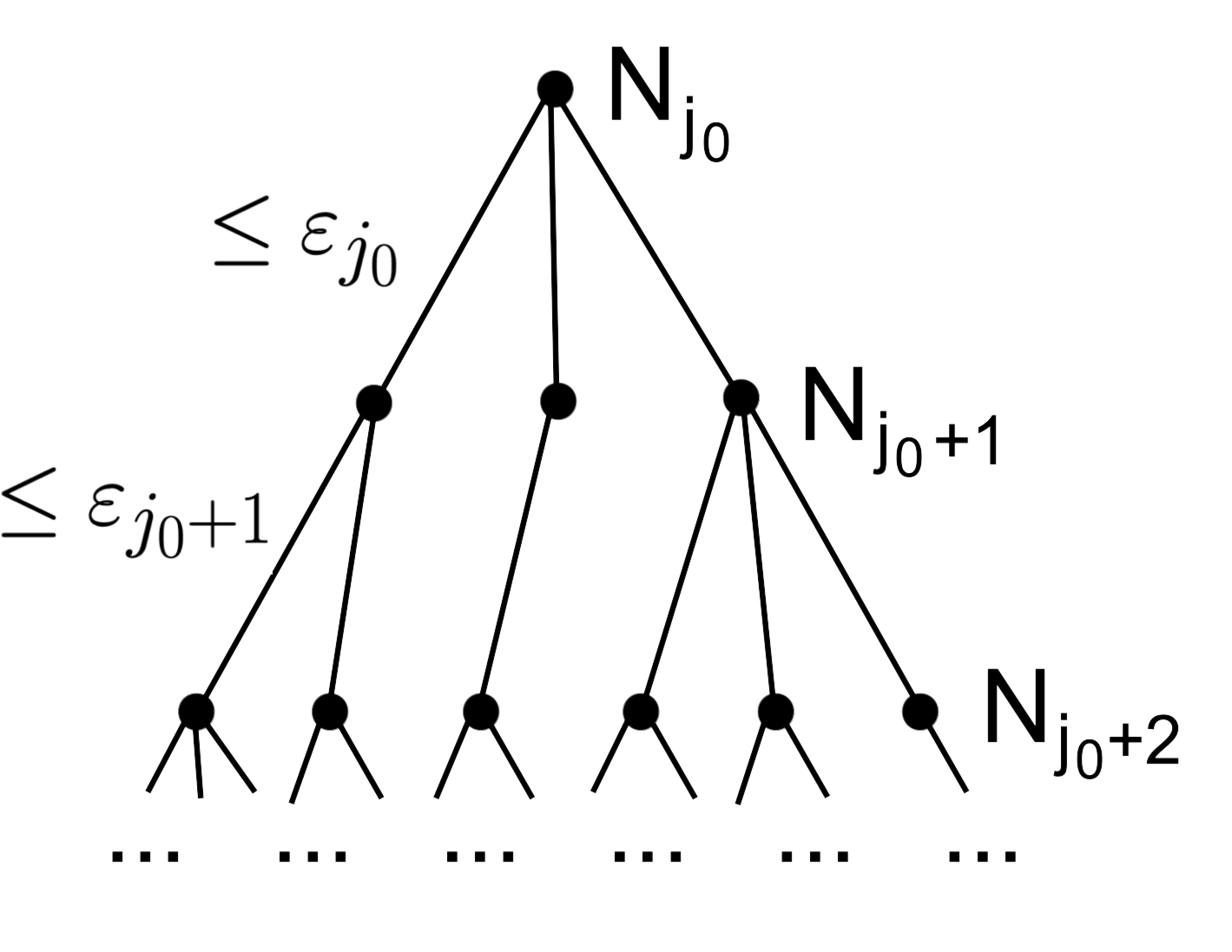
Figure 4. Chaining: construction of a spanning tree of a metric space.

If all the nets $\mathcal{N}_{j}$ that make up the levels of the tree $T_{0}$ are disjoint, then $T_{0}$ is a spanning tree of $T$. Assume that this is the case for time being.

Step 2: bounding the length of the tree. For each of the levels $j=j_{0}+1,j_{0}+2,\ldots$, the tree $T_{0}$ has $\mathinner{\!\left\lvert\mathcal{N}_{j}\right\rvert}$ edges connecting the points of level $j$ to the level $j-1$, and each such edge has length (weight) bounded by $\varepsilon_{j-1}$. So $\operatorname{MST}(T)$ is bounded by the sum of the lengths of the edges of $T_{0}$, i.e.

$$\operatorname{MST}(T)\leq\sum_{j=j_{0}+1}^{\infty}\varepsilon_{j-1}\mathinner{\!\left\lvert\mathcal{N}_{j}\right\rvert}.$$

Step 3: bounding the sum by the integral. Our choice $\varepsilon_{j}=2^{-j}$ yields $\varepsilon_{j-1}=4(\varepsilon_{j}-\varepsilon_{j+1})$. Moreover, our choice of $j_{0}$ yields $\mathinner{\!\left\lvert\mathcal{N}_{j}\right\rvert}\geq 2$ for all $j\geq j_{0}+1$, which implies $\mathinner{\!\left\lvert\mathcal{N}_{j}\right\rvert}\leq 2\left(\mathinner{\!\left\lvert\mathcal{N}_{j}\right\rvert}-1\right)$ for such $j$. Therefore

$$\operatorname{MST}(T) \leq 8\sum_{j=j_{0}+1}^{\infty}\left(\varepsilon_{j}-\varepsilon_{j+1}\right)\left(\mathinner{\!\left\lvert\mathcal{N}_{j}\right\rvert}-1\right)$$ (6.1)

$$=8\sum_{j=j_{0}+1}^{\infty}\int_{\varepsilon_{j+1}}^{\varepsilon_{j}}\left(N(T,\rho,\varepsilon_{j})-1\right)dx\quad\text{(since $\mathinner{\!\left\lvert\mathcal{N}_{j}\right\rvert}=N(T,\rho,\varepsilon_{j})$)}$$

$$\leq 8\int_{0}^{\infty}\left(N(T,\rho,x)-1\right)\,dx.$$

An application of Lemma 6.1 completes the proof.

Step 4: splitting. The argument above assumes that all levels $\mathcal{N}_{j}$ of the tree $T_{0}$ are disjoint. This assumption can be enforced by splitting the points of $T$. If, for example, a point $\omega\in\mathcal{N}_{j}$ is also used in $\mathcal{N}_{k}$ for some $k<j$, add to $T$ another a replica of $\omega$ – a point $\omega^{\prime}$ that has zero distance to $\omega$ and the same distances to all other points as $\omega$. Use $\omega$ in $\mathcal{N}_{j}$ and $\omega^{\prime}$ in $\mathcal{N}_{k}$. Preprocessing the metric space $(T,\rho)$ by such splitting yields a pseudometric space $(T^{\prime},\rho)$ in which all levels $\mathcal{N}_{j}$ are disjoint, and whose TSP is the same. ∎

Remark 6.4 (Integrating up to the diameter).

Note that $N(T,\rho,x)=1$ for any $x>\operatorname{diam}(T)$, since any single point makes an $x$-net of $T$ for such $x$. Therefore, the integrand in Theorem 6.3 vanishes for such $x$, and we have

$$\operatorname{TSP}(T)\leq 16\int_{0}^{\operatorname{diam}(T)}N(T,\rho,x)\,dx.$$ (6.2)

6.4. Folding

It is a simple observation that an interval of length $\operatorname{TSP}(T)$ can be embedded, or “folded”, into $T$:

Proposition 6.5 (Folding).

For any finite metric space $(T,\rho)$ there exists a finite subset $\Omega$ of the interval $[0,\operatorname{TSP}(T)]$ and a $1$-Lipschitz bijection $F\mathrel{\mathop{\mathchar 58\relax}}\Omega\to T$.

Heuristically, the map $F$ “folds” the interval $[0,\operatorname{TSP}(T)]$ into the shortest Hamiltonian path of the metric space $T$, see Figure 5. We can think of this as a space-filling curve of $T$.

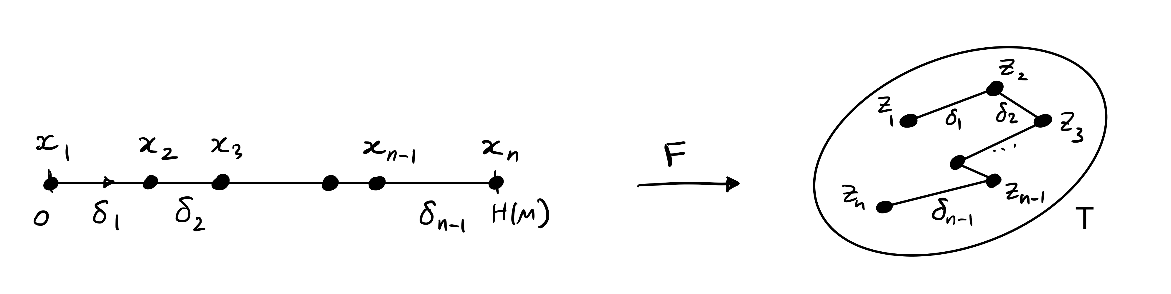
Figure 5. The map $F$ folds an interval $[0,\operatorname{TSP}(M)]$ into a Hamiltonian path (a “space-filling curve”) of the metric space $T$.

Proof.

Let us exploit the heuristic idea of folding. Fix a Hamiltonian cycle in $T$ of length $\operatorname{TSP}(T)$, whose existence is given by Lemma 6.2. Formally, this means that we can label the elements of the space as $T=\{z_{1},\ldots,z_{n}\}$ in such a way that the lengths

$$\delta_{i}=\rho\left(z_{i+1},z_{i}\right),\quad i=1,\ldots,n-1,$$

satisfy $\sum_{i=1}^{n-1}\delta_{i}\leq\operatorname{TSP}(T)$. Define $\Omega=\{x_{1},\ldots,x_{n}\}$ by

$$x_{1}=0;\quad x_{k}=\sum_{i=1}^{k-1}\delta_{i},\;k=2,\ldots,n.$$

Then all $x_{k}\leq\operatorname{TSP}(T)$, so $\Omega\subset[0,\operatorname{TSP}(T)]$ as claimed.

Note that for every $k=1,\ldots,n-1$ we have

$$\rho\left(z_{k+1},z_{k}\right)=\delta_{k}=x_{k+1}-x_{k}.$$

Then, for any integers $1\leq k\leq k+j\leq n$, triangle inequality and telescoping give

$$\rho\left(z_{k+j},z_{k}\right) \leq\rho\left(z_{k+j},z_{k+j-1}\right)+\rho\left(z_{k+j-1},z_{k+j-2}\right)+\cdots+\rho\left(z_{k+1},z_{k}\right)$$

$$=\left(x_{k+j}-x_{k+j-1}\right)+\left(x_{k+j-1}-x_{k+j-2}\right)+\cdots+\left(x_{k+1}-x_{k}\right)$$

$$=x_{k+j}-x_{k}.$$

This shows that the folding map $F\mathrel{\mathop{\mathchar 58\relax}}x_{k}\mapsto z_{k}$ is a bijection that satisfies

$$\rho\left(F(x),F(y)\right)\leq\mathinner{\!\left\lvert x-y\right\rvert}\quad\text{for all }x,y\in\Omega.$$

In other words, $F$ is $1$-Lipschitz. The proof is complete. ∎

7. A private measure on a metric space

We are ready to construct a private measure on an arbitrary compact metric space $(T,\rho)$. We do this as follows: (a) discretize $T$ replacing it with a finite $\delta$-net; (b) fold an interval of length $\operatorname{TSP}(T)$ onto $T$ using Proposition 6.5; and (c) using this folding, pushforward onto $T$ the private measure on the interval constructed in Section 5. The accuracy of the resulting private measure on $T$ is determined by the length of the interval $\operatorname{TSP}(T)$, which in turn can be expressed using the covering numbers of $T$ (Theorem 6.3).

7.1. Finite metric spaces

Let us start by extending Proposition 5.2 from a finite subset on $[0,1]$ to a finite subset of $(T,\rho)$.

Proposition 7.1 (Private measure on a finite metric space).

Let $(T,\rho)$ be a finite metric space and let $n=\mathinner{\!\left\lvert T\right\rvert}$. Let $\alpha>0$. There exists a randomized algorithm $\mathcal{B}$ that takes a probability measure $\mu$ on $T$ as an input and returns a probability measure $\nu$ on $T$ as an output, and with the following two properties.

1. (Privacy): the algorithm $\mathcal{B}$ is $\alpha$-metrically private in the TV metric.

2. (Accuracy): for any input measure $\mu$, the expected accuracy of the output measure $\nu$ in the Wasserstein distance is

   $$\operatorname{\mathbb{E}}W_{1}(\nu,\mu)\leq\frac{C\log^{\frac{3}{2}}n}{\alpha}\,\operatorname{TSP}(T).$$

Proof.

Applying Folding Proposition 6.5, we obtain an $n$-element subset $\Omega\subset[0,\operatorname{TSP}(T)]$ and a $1$-Lipschitz bijection $F\mathrel{\mathop{\mathchar 58\relax}}\Omega\to T$. Applying Proposition 5.2 and rescaling by the factor $\operatorname{TSP}(T)$, we obtain an $\alpha$-metrically private algorithm $\mathcal{B}$ that transforms a probability measure $\mu$ on $\Omega$ into a probability measure $\nu$ on $\Omega$, and whose accuracy is

$$\operatorname{\mathbb{E}}W_{1}(\nu,\mu)\leq\frac{C\log^{\frac{3}{2}}n}{\alpha}\,\operatorname{TSP}(T).$$ (7.1)

Define a new metric $\bar{\rho}$ on $\Omega$ by $\bar{\rho}(x,y)=\rho\left(F(x),F(y)\right)$. Since $F$ is $1$-Lipschitz, we have $\bar{\rho}(x,y)\leq\mathinner{\!\left\lvert x-y\right\rvert}$. Note that the Wasserstein distance can only become smaller if the underlying metric is replaced by a smaller metric. Therefore, the bound (7.1), which holds with respect to the usual metric $\mathinner{\!\left\lvert x-y\right\rvert}$ on $\Omega$, automatically holds with respect to the smaller metric $\bar{\rho}(x,y)$.

It remains to note that $(\Omega,\bar{\rho})$ is isometric to $(T,\rho)$. So the accuracy result (7.1), which as we saw holds in $(\Omega,\bar{\rho})$, automatically transfers to $(T,\rho)$ (by considering the pushforward measure). ∎

7.2. General metric spaces

Quantization allows us to pass from discrete metric spaces to general spaces. A similar technique was used in Section 5.2 for the interval $[0,1]$. We will repeat it here for a general metric space.

7.2.1. Quantization

Fix $\delta>0$ and let $\mathcal{N}=\{\omega_{1},\ldots,\omega_{n}\}$ be a $\delta$-net of $T$ such that $n=\mathinner{\!\left\lvert\mathcal{N}\right\rvert}=N(T,\rho,\delta)$. Consider the proximity partition

$$T=I_{1}\cup\cdots\cup I_{n}$$

where we put a point $x\in T$ into $I_{i}$ if $x$ is closer to $\omega_{i}$ that to any other points in $\mathcal{N}$. (We break any ties arbitrarily.)

We can quantize any signed measure $\nu$ on $T$ by defining

$$\nu_{\mathcal{N}}\left(\{\omega_{i}\}\right)=\nu(I_{i}),i=1,\ldots,n.$$

Obviously, $\nu_{\mathcal{N}}$ is a signed measure on $\mathcal{N}$. Moreover, if $\nu$ is a measure, then so is $\nu_{\mathcal{N}}$. And if $\nu$ is a probability measure, then so is $\nu_{\mathcal{N}}$. In the latter case, it follows from the construction that

$$W_{1}(\nu,\nu_{\mathcal{N}})\leq\delta.$$ (7.2)

(By definition of the net, transporting any point $x$ to the closest point $\omega_{i}$ covers distance at most $\delta$.) Furthermore, Lemma 5.3 easily generalizes and yields

$$\mathinner{\!\left\lVert\nu_{\mathcal{N}}\right\rVert}_{\mathrm{TV}}\leq\mathinner{\!\left\lVert\nu\right\rVert}_{\mathrm{TV}}.$$ (7.3)

Finally, let us bound the TSP of the net $\mathcal{N}$ using Theorem 6.3. We trivially have $N(\mathcal{N},\rho,x)\leq\mathinner{\!\left\lvert\mathcal{N}\right\rvert}=N(T,\rho,\delta)$ for any $x>0$. Moreover, since $\mathcal{N}\subset T$, we also have $N(\mathcal{N},\rho,x)\leq N(T,\rho,x/2)$, see [48, Exercise 4.2.10]. Using the former bound for $x<2\delta$ and the latter bound for $x\geq 2\delta$ and applying (6.2), we obtain

$$\operatorname{TSP}(\mathcal{N}) \lesssim\int_{0}^{\operatorname{diam}(\mathcal{N})}N(\mathcal{N},\rho,x)\,dx$$

$$\leq 2\delta N(T,\rho,\delta)+\int_{2\delta}^{\operatorname{diam}(T)}N(T,\rho,x/2)\,dx$$

$$=2\left(\delta N(T,\rho,\delta)+\int_{\delta}^{\operatorname{diam}(T)/2}N(T,\rho,x)\,dx\right)$$

$$\leq 2\left(2\int_{\delta/2}^{\delta}N(T,\rho,x)\,dx+\int_{\delta}^{\operatorname{diam}(T)/2}N(T,\rho,x)\,dx\right)$$

$$\leq 4\int_{\delta/2}^{\operatorname{diam}(T)/2}N(T,\rho,x)\,dx.$$ (7.4)

7.2.2. A private measure on a general metric space

Theorem 7.2 (Private measure on a metric space).

Let $(T,\rho)$ be a compact metric space. Let $\alpha,\delta>0$. There exists a randomized algorithm $\mathcal{A}$ that takes a probability measure $\mu$ on $T$ as an input and returns a finitely-supported probability measure $\nu$ on $T$ as an output, and with the following two properties.

1. (Privacy): the algorithm $\mathcal{A}$ is $\alpha$-metrically private in the TV metric.

2. (Accuracy): for any input measure $\mu$, the expected accuracy of the output measure $\nu$ in the Wasserstein distance is

   $$\operatorname{\mathbb{E}}W_{1}(\nu,\mu)\leq 2\delta+\frac{C}{\alpha}\log^{\frac{3}{2}}\left(N(T,\rho,\delta)\right)\int_{\delta}^{\operatorname{diam}(T)}N(T,\rho,x)\,dx.$$

Proof.

Preprocess the input measure $\mu$ by quantizing as in the previous subsection, and feed the quantized measure $\mu_{\mathcal{N}}$ into the algorithm $\mathcal{B}$ of Proposition 7.1 for the metric space $(\mathcal{N},\rho)$.

The contraction property (7.3) ensures that

$$\mathinner{\!\left\lVert\mu_{\mathcal{N}}-\mu^{\prime}_{\mathcal{N}}\right\rVert}_{\mathrm{TV}}\leq\mathinner{\!\left\lVert\mu-\mu^{\prime}\right\rVert}_{\mathrm{TV}}$$

for any two input measures $\mu$ and $\mu^{\prime}$. This and the privacy property in Proposition 7.1 for measures on $\mathcal{N}$ guarantee that quantization does not destroy privacy, i.e. the algorithm $\mathcal{A}\mathrel{\mathop{\mathchar 58\relax}}\mu\mapsto\mathcal{B}(\mu_{\mathcal{N}})$ is still $\alpha$-metrically private as claimed.

Next, the accuracy property in Proposition 7.1 for the measure $\mu_{\mathcal{N}}$ on $\mathcal{N}$ gives

$$\operatorname{\mathbb{E}}W_{1}\left(\mathcal{B}(\mu_{\mathcal{N}}),\mu_{\mathcal{N}}\right)\leq\frac{C}{\alpha}\log^{\frac{3}{2}}(N(T,\rho,\delta))\,\operatorname{TSP}(\mathcal{N}).$$

Moreover, the accuracy of quantization (7.2) states that $W_{1}(\mu,\mu_{\mathcal{N}})\leq\delta$. By triangle inequality, we conclude that

$$\operatorname{\mathbb{E}}W_{1}\left(\mathcal{B}(\mu_{\mathcal{N}}),\mu\right)\leq\delta+\frac{C}{\alpha}\log^{\frac{3}{2}}(N(T,\rho,\delta))\,\operatorname{TSP}(\mathcal{N}).$$

Thus, by (7.4),

$$\operatorname{\mathbb{E}}W_{1}\left(\mathcal{B}(\mu_{\mathcal{N}}),\mu\right)\leq\delta+\frac{C}{\alpha}\log^{\frac{3}{2}}(N(T,\rho,\delta))\,\int_{\delta/2}^{\operatorname{diam}(T)/2}N(T,\rho,x)\,dx.$$

Since $N(T,\rho,2\delta)\leq N(T,\rho,\delta)$, replacing $\delta$ by $2\delta$ completes the proof of the theorem. ∎

7.3. Private synthetic data

The output of the algorithm $\mathcal{A}$ in Theorem 7.2 is a finitely-supported probability measure $\nu$ on $T$. Quantization allows to transform $\nu$ into an empirical measure

$$\mu_{Y}=\frac{1}{m}\sum_{i=1}^{m}\delta_{Y_{i}}$$ (7.5)

where $Y_{1},\ldots,Y_{m}$ is some finite sequence of elements of $T$, in which repetitions are allowed. In other words, we can make the output of our algorithm a synthetic data $Y=(Y_{1},\ldots,Y_{m})$. Let us record this observation.

Corollary 7.3 (Outputting an empirical measure).

Let $(T,\rho)$ be a compact metric space. Let $\alpha,\delta>0$. There exists a randomized algorithm $\mathcal{A}$ that takes a probability measure $\mu$ on $T$ as an input and returns $Y=(Y_{1},\ldots,Y_{m})\in T^{m}$ for some $m$ as an output, and with the following two properties.

1. (Privacy): the algorithm $\mathcal{A}$ is $\alpha$-metrically private in the TV metric.

2. (Accuracy): for any input measure $\mu$, the expected accuracy of the empirical measure $\mu_{Y}$ in the Wasserstein distance is

   $$\operatorname{\mathbb{E}}W_{1}\left(\mu_{Y},\mu\right)\leq 3\delta+\frac{C}{\alpha}\log^{\frac{3}{2}}\left(N(T,\rho,\delta)\right)\int_{\delta}^{\operatorname{diam}(T)}N(T,\rho,x)\,dx.$$

Proof.

Since the output probability measure $\nu$ in Theorem 7.2 is finitely supported, it has the form

$$\nu=\sum_{i=1}^{r}w_{i}\,\delta_{Y_{i}}$$

for some natural number $r$, positive weights $w_{i}$ and elements $R_{i}\in T$.

Let us quantize the weights $w_{i}$ by the uniform quantizer with step $1/m$ where $m$ is a large integer. Namely, set

$$q(w_{i})\coloneqq\frac{\lfloor m\,w_{i}\rfloor}{m}.$$

Obviously, the total quantization error satisfies

$$\kappa\coloneqq\sum_{i=1}^{r}\left(w_{i}-q(w_{i})\right)\in[0,r/m].$$ (7.6)

To make the quantized weights a probability measure, let us add the total quantization error to any given weight, say the first. Thus, define

$$w^{\prime}_{1}\coloneqq q(w_{1})+\kappa\quad\text{and}\quad w^{\prime}_{i}\coloneqq q(w_{i}),\;i=2,\ldots,r$$

and set

$$\nu^{\prime}\coloneqq\sum_{i=1}^{r}w^{\prime}_{i}\,\delta_{Y_{i}}.$$

Note the three key properties of $\nu^{\prime}$. First, since the weights $w^{\prime}_{i}$ sum to one, $\nu^{\prime}$ is a probability measure. Second, since $\nu^{\prime}$ is obtained from $\nu$ by transporting a total mass of $\kappa$ across the metric space $T$, we have

$$W_{1}(\nu,\nu^{\prime})\leq\kappa\cdot\operatorname{diam}(T)\leq\frac{r}{m}\cdot\operatorname{diam}(T)\leq\delta$$

where the second inequality follows from (7.6) and the last one by choosing $m$ large enough. Third, all quantized weights $q(w_{i})$ belong to $\frac{1}{m}\mathbb{Z}$ by definition. Thus, $\kappa=1-\sum_{i=1}^{r}q(w_{i})$ is also in $\frac{1}{m}\mathbb{Z}$. Therefore, all weights $w^{\prime}_{i}$ are in $\frac{1}{m}\mathbb{Z}$, too. Hence, $w^{\prime}_{i}=m_{i}/m$ for some nonnegative integers $m_{i}$. In other words,

$$\nu^{\prime}=\frac{1}{m}\sum_{i=1}^{r}m_{i}\,\delta_{Y_{i}}.$$

Since $\nu^{\prime}$ is a probability measure, we must have $\sum_{i=1}^{r}m_{i}=m$. Redefine the sequence $Y_{1},\ldots,Y_{m}$ by repeating each element $Y_{i}$ of the sequence $Y_{1},\ldots,Y_{r}$ exactly $m_{i}$ times. Thus $\nu^{\prime}=\frac{1}{m}\sum_{i=1}^{m}\delta_{Y_{i}}$, as required. ∎

Corollary 7.3 allows us to transform any true data $X=(X_{1},\ldots,X_{n})$ into a private synthetic data $Y=(Y_{1},\ldots,Y_{m})$. To do this, feed the algorithm $\mathcal{A}$ with the empirical measure on the true data $\mu_{X}=\frac{1}{n}\sum_{i=1}^{n}\delta_{X_{i}}$. Recall from Lemma 4.1 that if the algorithm $\mathcal{A}$ is $\alpha$-metrically private for $\alpha=\varepsilon n$, then the algorithm $X\mapsto Y=\mathcal{A}(\mu_{X})$ yields $\varepsilon$-differential private synthetic data. Let us record this observation:

Corollary 7.4 (Differentially private synthetic data).

Let $(T,\rho)$ be a compact metric space. Let $\varepsilon,\delta>0$. There exists a randomized algorithm $\mathcal{A}$ that takes true data $X=(X_{1},\ldots,X_{n})\in T^{n}$ as an input and returns synthetic data $Y=(Y_{1},\ldots,Y_{m})\in T^{m}$ for some $m$ as an output, and with the following two properties.

1. (Privacy): the algorithm $\mathcal{A}$ is $\varepsilon$-differentially private.

2. (Accuracy): for any true data $X$, the expected accuracy of the synthetic data $Y$ is

   $$\operatorname{\mathbb{E}}W_{1}\left(\mu_{Y},\mu_{X}\right)\leq 3\delta+\frac{C}{\varepsilon n}\log^{\frac{3}{2}}\left(N(T,\rho,\delta)\right)\int_{\delta}^{\operatorname{diam}(T)}N(T,\rho,x)\,dx,$$

   where $\mu_{X}$ and $\mu_{Y}$ denote the corresponding empirical measures.

An interested reader may now skip to Section 9.1 where we illustrate Corollary 7.4 for a specific example of the metric space, namely the $d$-dimensional cube $T=[0,1]^{d}$.

Remark 7.5 (A computationally effective algorithm).

We will present a detailed discussion of the algorithmic aspects of the proposed synthetic data generation method in a forthcoming paper. Here, we only mention that our algorithm works in polynomial time with respect to the cardinality of the dataset. To be more precise, assuming that the input measure $\mu$ is given by an oracle for any set $A$, the oracle gives us $\mu(A)$ and we need a polynomial number of calls to such an oracle.

8. A lower bound

This section is devoted to impossibility results, which yield lower bounds on the accuracy of any private measure on a general metric space $(T,\rho)$. While there may be a gap between our upper and lower bounds for general metric spaces, we will see in Section 9 that this gap vanishes asymptotically for spaces of Minkowski dimension $d$.

The proof of the lower bound uses the geometric method pioneered by Hardt and Talwar [25]. A lower bound is more convenient to express in terms of packing rather than covering numbers. Recall that the packing number ${N_{\textrm{pack}}}(T,\rho,\varepsilon)$ of a compact metric space $(T,\rho)$ is defined as the largest cardinality of an $\varepsilon$-separated subset of $T$. The covering and packing numbers are equivalent up to a factor of $2$:

$${N_{\textrm{pack}}}(T,\rho,2\varepsilon)\leq N(T,\rho,\varepsilon)\leq{N_{\textrm{pack}}}(T,\rho,\varepsilon),$$ (8.1)

see [48, Lemma 4.2.8]. Thus, in all results of this section, packing numbers can be replaced by covering numbers at the cost of changing absolute constants.

8.1. A master lower bound

We first prove a general result that establishes limitations of metric privacy. To understand this statement better, it may be helpful to assume that $\mathcal{M}_{0}=\mathcal{M}_{1}$ and $\rho_{0}=\rho_{1}$ in the first reading.

Proposition 8.1 (A master lower bound).

Let $\mathcal{M}_{0}\subset\mathcal{M}_{1}$ be two subsets, and let $\rho_{i}$ be a metric on $\mathcal{M}_{i}$, $i=0,1$. Assume that for some $t,\alpha>0$ we have

$$\operatorname{diam}(\mathcal{M}_{0},\rho_{0})\leq 1\quad\text{and}\quad{N_{\textrm{pack}}}(\mathcal{M}_{0},\rho_{1},t)>2e^{\alpha}.$$

Then, for any randomized algorithm $\mathcal{A}\mathrel{\mathop{\mathchar 58\relax}}\mathcal{M}_{0}\to\mathcal{M}_{1}$ that is $\alpha$-metrically private with respect to the metric $\rho_{0}$, there exists $x\in\mathcal{M}_{0}$ such that

$$\operatorname{\mathbb{E}}\rho_{1}\left(\mathcal{A}(x),x\right)>t/4.$$

Proof.

For contradiction, assume that

$$\operatorname{\mathbb{E}}\rho_{1}\left(\mathcal{A}(x),x\right)\leq t/4,$$ (8.2)

for all $x\in\mathcal{M}_{0}$. Let $\mathcal{N}$ be a $t$-separated subset of the metric space $(\mathcal{M}_{0},\rho_{1})$ with cardinality

$$\mathinner{\!\left\lvert\mathcal{N}\right\rvert}>2e^{\alpha}.$$ (8.3)

The separation condition implies that the balls $B(y,\rho_{1},t/2)$ centered at the points $y\in\mathcal{N}$ and with radii $t/2$ are all disjoint.

Fix any reference point $y\in\mathcal{M}_{0}$. The disjointness of the balls yields

$$\sum_{x\in\mathcal{N}}\mathbb{P}\left\{\mathcal{A}(y)\in B(x,\rho_{1},t/2)\rule{0.0pt}{8.53581pt}\right\}\leq 1.$$ (8.4)

On the other hand, by the definition of $\alpha$-metric privacy, for each $x\in\mathcal{N}$ we have:

$$\mathbb{P}\left\{\mathcal{A}(y)\in B(x,\rho_{1},t/2)\rule{0.0pt}{8.53581pt}\right\}\geq\exp\left[-\alpha\rho_{0}(x,y)\right]\cdot\mathbb{P}\left\{\mathcal{A}(x)\in B(x,\rho_{1},t/2)\rule{0.0pt}{8.53581pt}\right\}.$$

The diameter assumption yields $\rho_{0}(x,y)\leq 1$. Furthermore, using the assumption (8.2) and Markov’s inequality, we obtain

$$\mathbb{P}\left\{\mathcal{A}(x)\in B(x,\rho_{1},t/2)\rule{0.0pt}{8.53581pt}\right\}=\mathbb{P}\left\{\rho_{1}\left(\mathcal{A}(x),x\right)\leq t/2\rule{0.0pt}{8.53581pt}\right\}\geq\frac{1}{2}.$$

Combining the two bounds gives

$$\mathbb{P}\left\{\mathcal{A}(y)\in B(x,\rho_{1},t/2)\rule{0.0pt}{8.53581pt}\right\}\geq\frac{1}{2e^{\alpha}}.$$

Substitute this into (8.4) to get

$$\sum_{x\in\mathcal{N}}\frac{1}{2e^{\alpha}}\leq 1.$$

In other words, we conclude that $\mathinner{\!\left\lvert\mathcal{N}\right\rvert}\leq 2e^{\alpha}$, which contradicts (8.3). The proof is complete. ∎

8.2. Metric entropy of the space of probability measures

For a given compact metric space $(T,\rho)$, we denote by $\mathcal{M}(T)$ the collection of all Borel probability measures on $T$. We are going to apply Proposition 8.1 for $\mathcal{M}_{0}=\mathcal{M}_{1}=\mathcal{M}(T)$, for $\rho_{1}=$ Wasserstein metric and $\rho_{0}=$ TV metric. That proposition requires a lower bound on the packing number ${N_{\textrm{pack}}}\left(\mathcal{M}(T),W_{1},t/3\right)$. In the next lemma, we relate this packing number to that of $(T,\rho)$. Essentially, it says that if $T$ is large, then there are a lot of probability measures on $T$.

Proposition 8.2 (Metric entropy of the space of probability measures).

For any compact metric space $(T,\rho)$ and every $t>0$, we have

$${N_{\textrm{pack}}}\left(\mathcal{M}(T),W_{1},t/3\right)\geq\exp\left(c{N_{\textrm{pack}}}(T,\rho,t)\right),$$

where $c>0$ is a universal constant.

The proof will use the following lemma.

Lemma 8.3 (A lower bound on the Wasserstein distance).

Let $(T,\rho)$ be a $t$-separated compact metric space. Then, for any pair of probability measures $\mu,\nu$ on $T$, we have

$$W_{1}(\mu,\nu)\geq\mu(B^{c})\,t\quad\text{where}\quad B=\operatorname{supp}(\nu).$$

Proof.

Suppose that $\gamma$ is a coupling of $\mu$ and $\nu$. Since $\nu$ is supported on $B$, we have $\gamma(B^{c}\times B^{c})\leq\gamma(T\times B^{c})=\nu(B^{c})=0$, which means that $\gamma(B^{c}\times B^{c})=0$. Therefore

$$\gamma(B^{c}\times B)=\gamma(B^{c}\times T)-\gamma(B^{c}\times B^{c})=\mu(B^{c}).$$

Since the sets $B^{c}$ and $B$ are disjoint, the separation assumption implies that $\rho(x,y)>t$ for all pairs $x\in B^{c}$ and $y\in B$. Thus,

$$\int_{T\times T}\rho(x,y)\;d\gamma(x,y)\geq\int_{B^{c}\times B}\rho(x,y)\;d\gamma(x,y)\geq t\gamma(B^{c}\times B)=t\mu(B^{c}).$$

Since this holds for all coupling $\gamma$ of $\mu$ and $\nu$, the result follows. ∎

Lemma 8.4 (Many different measures).

Let $(\mathcal{N},\rho)$ be a $t$-separated compact metric space, and assume that $\mathinner{\!\left\lvert\mathcal{N}\right\rvert}\geq 2n$ for some $n\in\mathbb{N}$. Then there exists a family of at least $\exp(cn)$ empirical measures on $n$ points of $T$ that are pairwise $t/3$-separated in the Wasserstein distance, where $c>0$ is a universal constant.

Proof.

Let $\mu=n^{-1}\sum_{i=1}^{n}\delta_{X_{i}}$ and $\nu=n^{-1}\sum_{i=1}^{n}\delta_{Y_{i}}$ be two independent random empirical measures on $T$. Let us condition on $\nu$ and denote $B=\operatorname{supp}(\nu)$. Then

$$\mu(B^{c})=\frac{1}{n}\sum_{i=1}^{n}{\textbf{1}}_{\{X_{i}\in B^{c}\}}.$$

Now, ${\textbf{1}}_{\{X_{i}\in B^{c}\}}$ are i.i.d. Bernoulli random variables that take value $1$ with probability

$$\mathbb{P}\left\{X_{i}\in B^{c}\rule{0.0pt}{8.53581pt}\right\}=\frac{\mathinner{\!\left\lvert B^{c}\right\rvert}}{\mathinner{\!\left\lvert\mathcal{N}\right\rvert}}\geq\frac{1}{2},$$

since by construction we have $\mathinner{\!\left\lvert B\right\rvert}\leq n$ and by assumption $\mathinner{\!\left\lvert\mathcal{N}\right\rvert}\geq 2n$. Then, applying Chernoff inequality (see [48, Exercise 2.3.2]), we conclude that $\mu(B^{c})>1/3$ with probability bigger than $1-e^{-5cn}$, where $c>0$ is a universal constant. Lemma 8.3 yields that $W_{1}(\mu,\nu)>t/3$.

Now consider a sequence $\mu_{1},\ldots,\mu_{K}$ of independent random empirical measures on $T$. Using the result above and taking a union bound we conclude that, with probability at least $1-\binom{K}{2}e^{-5cn}$, the inequality $W_{1}(\mu_{i},\mu_{j})>t/3$ holds for all pairs of distinct indices $i,j\in\{1,\ldots,K\}$. Choosing $K=\lceil e^{cn}\rceil$ makes $K$ between $e^{cn}$ (as claimed) and $e^{2cn}$. Thus, the success probability is more than $1-(e^{2cn})^{2}e^{-5cn}$, which is positive. The existence of the required family of measures follows. ∎

Proof of Proposition 8.2.

Let $\mathcal{N}\subset T$ be a $t$-separated subset of cardinality $\mathinner{\!\left\lvert\mathcal{N}\right\rvert}={N_{\textrm{pack}}}(T,\rho,t)$. Lemma 8.4 implies the existence of a set of at least $\exp(c\mathinner{\!\left\lvert\mathcal{N}\right\rvert})$ probability measures on $T$ that is $(t/3)$-separated in the Wasserstein distance. In other words, we have ${N_{\textrm{pack}}}\left(\mathcal{M}(T),W_{1},t/3\right)\geq\exp(c\mathinner{\!\left\lvert\mathcal{N}\right\rvert})$. Proposition 8.2 is proved. ∎

8.3. Lower bounds for private measures and synthetic data

Now we are ready to prove the two main lower bounds on the accuracy for (a) metrically private measures and (b) differential private data.

Theorem 8.5 (Private measure: a lower bound).

Let $(T,\rho)$ be a compact metric space. Assume that for some $t>0$ and $\alpha\geq 1$ we have

$${N_{\textrm{pack}}}(T,\rho,t)>C\alpha.$$

Then, for any randomized algorithm $\mathcal{A}$ that takes a probability measure $\mu$ on $T$ as an input and returns a probability measure $\nu$ on $T$ as an output and that is $\alpha$-metrically private with respect to the TV metric, there exists $\mu$ such that

$$\operatorname{\mathbb{E}}W_{1}(\nu,\mu)>t/12.$$

Proof.

The assumption on the packing number for a sufficiently large constant $C$ and Proposition 8.2 yield

$${N_{\textrm{pack}}}\left(\mathcal{M}(T),W_{1},t/3\right)\geq e^{2\alpha}>2e^{\alpha}.$$

Next, apply Proposition 8.1 with $t/3$ instead of $t$, and for $\mathcal{M}_{0}=\mathcal{M}_{1}=\mathcal{M}(T)$, setting $\rho_{1}$ and $\rho_{0}$ to be the Wasserstein and the TV metrics, respectively. The required conclusion follows. ∎

Theorem 8.6 (Synthetic data: a lower bound).

There exists an absolute constant $n_{0}$ such that the following holds. Let $(T,\rho)$ be a compact metric space. Assume that for some $t>0$ and and some integer $n>n_{0}$ we have

$${N_{\textrm{pack}}}(T,\rho,t)>2n.$$

Then, for any $c$-differentially private randomized algorithm $\mathcal{A}$ that takes true data $X=(X_{1},\ldots,X_{n})\in T^{n}$ as an input and returns synthetic data $Y=(Y_{1},\ldots,Y_{m})\in T^{m}$ for some $m$ as an output, there exists input data $X$ such that

$$\operatorname{\mathbb{E}}W_{1}(\mu_{Y},\mu_{X})>t/12,$$

where $\mu_{X}$ and $\mu_{Y}$ denote the empirical measures on $X$ and $Y$.

Proof.

First note that a version of Proposition 8.2 holds for empirical measures. Namely, denote the set of all empirical measures on $n$ points of $T$ by $\mathcal{M}_{n}(T)$. If ${N_{\textrm{pack}}}(T,\rho,t)>2n$ then we claim that

$${N_{\textrm{pack}}}\left(\mathcal{M}_{n}(T),W_{1},t/3\right)>2e^{c_{1}n}.$$ (8.5)

To see this, let $\mathcal{N}\subset T$ be a $t$-separated subset of cardinality $\mathinner{\!\left\lvert\mathcal{N}\right\rvert}>2n$. Lemma 8.4 implies the existence of a set of at least $e^{cn}\geq 2e^{c_{1}n}$ members of $\mathcal{M}_{n}(T)$ that is $(t/3)$-separated in the Wasserstein distance. The claim (8.5) follows.

In preparation to apply Proposition 8.1, consider the sets $\mathcal{M}_{0}\coloneqq T^{n}$ and $\mathcal{M}_{1}\coloneqq\cup_{k=1}^{\infty}T^{k}$. Consider the normalized Hamming metric

$$\rho_{0}(X,X^{\prime})=\frac{1}{n}\mathinner{\!\left\lvert\{i\in[n]\mathrel{\mathop{\mathchar 58\relax}}\;X_{i}\neq X^{\prime}_{i}\}\right\rvert}$$

on $\mathcal{M}_{0}$, and the Wasserstein metric

$$\rho_{1}(X,X^{\prime})=W_{1}(\mu_{X},\mu_{X^{\prime}})$$

on $\mathcal{M}_{1}$. Then we clearly have $\operatorname{diam}(\mathcal{M}_{0},\rho_{0})\leq 1$, and (8.5) is equivalent to ${N_{\textrm{pack}}}(\mathcal{M}_{0},\rho_{1},t/3)>2e^{c_{1}n}$.

If $\mathcal{A}\mathrel{\mathop{\mathchar 58\relax}}\mathcal{M}_{0}\to\mathcal{M}_{1}$ is a $c$-differentially private algorithm, then $\mathcal{A}$ is $(cn)$-metrically private in the metric $\rho_{0}$ due to Lemma 2.3. Applying Proposition 8.1 with $t/3$ instead of $t$ and $\alpha=c_{1}n$, we obtain the required conclusion. ∎

9. Examples and asymptotics

9.1. A private measure on the unit cube

Let us work out the bound of Theorem 7.2 for a concrete example: the $d$-dimensional unit cube equipped with the $\ell^{\infty}$ metric, i.e. $(T,\rho)=([0,1]^{d},\,\mathinner{\!\left\lVert\cdot\right\rVert}_{\infty})$. The covering numbers satisfy

$$N(T,\mathinner{\!\left\lVert\cdot\right\rVert}_{\infty},x)\leq(1/x)^{d},\quad x>0,$$

since the set $x\mathbb{Z}^{d}\cap[0,1)^{d}$ forms an $x$-net of $T$. Thus the accuracy is

$$\operatorname{\mathbb{E}}W_{1}(\nu,\mu)\lesssim\delta+\frac{\log^{\frac{3}{2}}(1/\delta)}{\alpha}\int_{\delta}^{1}(1/x)^{d}\,dx\lesssim\delta+\frac{\log^{\frac{3}{2}}(1/\delta)}{\alpha}\cdot(1/\delta)^{d-1}$$

if $d\geq 2$. Optimizing in $\delta$ yields

$$\operatorname{\mathbb{E}}W_{1}(\nu,\mu)\lesssim\Big{(}\frac{\log^{\frac{3}{2}}\alpha}{\alpha}\Big{)}^{1/d},$$

which wonderfully extends Theorem 5.4 for $d=1$. Combining the two results, for $d=1$ and $d=2$, we obtain the following general result:

Corollary 9.1 (Private measure on the cube).

Let $d\in\mathbb{N}$ and $\alpha\geq 2$. There exists a randomized algorithm $\mathcal{A}$ that takes a probability measure $\mu$ on $[0,1]^{d}$ as an input and returns a finitely-supported probability measure $\nu$ on $[0,1]^{d}$ as an output, and with the following two properties.

1. (Privacy): the algorithm $\mathcal{A}$ is $\alpha$-metrically private in the TV metric.

2. (Accuracy): for any input measure $\mu$, the expected accuracy of the output measure $\nu$ in the Wasserstein distance is

   $$\operatorname{\mathbb{E}}W_{1}(\nu,\mu)\leq C\Big{(}\frac{\log^{\frac{3}{2}}\alpha}{\alpha}\Big{)}^{1/d}.$$

Similarly, by invoking Corollary 7.4, we obtain $\varepsilon$-differential privacy for synthetic data:

Corollary 9.2 (Private synthetic data in the cube).

Let $d,n\in\mathbb{N}$ and $\varepsilon>0$. There exists a randomized algorithm $\mathcal{A}$ that takes true data $X=(X_{1},\ldots,X_{n})\in([0,1]^{d})^{n}$ as an input and returns synthetic data $Y=(Y_{1},\ldots,Y_{m})\in([0,1]^{d})^{m}$ for some $m$ as an output, and with the following two properties.

1. (Privacy): the algorithm $\mathcal{A}$ is $\varepsilon$-differentially private.

2. (Accuracy): for any true data $X$, the expected accuracy of the synthetic data $Y$ is

   $$\operatorname{\mathbb{E}}W_{1}\left(\mu_{Y},\mu_{X}\right)\leq C\Big{(}\frac{\log^{\frac{3}{2}}(\varepsilon n)}{\varepsilon n}\Big{)}^{1/d},$$

   where $\mu_{X}$ and $\mu_{Y}$ denote the corresponding empirical measures.

The two results above are nearly sharp. Indeed, let us work out the lower bound for the cube, using Theorem 8.5. The covering numbers satisfy

$${N_{\textrm{pack}}}(T,\mathinner{\!\left\lVert\cdot\right\rVert}_{\infty},x)\geq(c/x)^{d},\quad x>0,$$

which again can be seen by considering a rescaled integer grid. Setting $t=c/(2C\alpha)^{1/d}$ we get $N(T,\mathinner{\!\left\lVert\cdot\right\rVert}_{\infty},t)>C\alpha$. Hence

$$\operatorname{\mathbb{E}}W_{1}(\nu,\mu)>t/12\gtrsim(1/\alpha)^{1/d},$$

which matches the upper bound in Corollary 9.1 up to a logarithmic factor. Let us record this result.

Corollary 9.3 (Private measure on the cube: a lower bound).

Let $d\in\mathbb{N}$ and $\alpha\geq 2$. Then, for any randomized algorithm $\mathcal{A}$ that takes a probability measure $\mu$ on $[0,1]^{d}$ as an input and returns a probability measure $\nu$ on $[0,1]^{d}$ as an output, and that is $\alpha$-metrically private with respect to the TV metric, there exists $\mu$ such that

$$\operatorname{\mathbb{E}}W_{1}(\nu,\mu)>c\Big{(}\frac{1}{\alpha}\Big{)}^{1/d}.$$

In a similar way, by invoking the lower bound in Theorem 8.6, we obtain the following nearly matching lower bound for Corollary 9.2:

Corollary 9.4 (Private synthetic data in the cube: a lower bound).

Let $d,n\in\mathbb{N}$. Then, for any $c$-differentially private randomized algorithm $\mathcal{A}$ that takes true data $X=(X_{1},\ldots,X_{n})\in([0,1]^{d})^{n}$ as an input and returns synthetic data $Y=(Y_{1},\ldots,Y_{m})\in([0,1]^{d})^{m}$ for some $m$ as an output, there exists input data $X$ such that

$$\operatorname{\mathbb{E}}W_{1}(\nu_{Y},\mu_{X})>c\Big{(}\frac{1}{n}\Big{)}^{1/d}.$$

where $\mu_{X}$ and $\mu_{Y}$ denotes the empirical measures on $X$ and $Y$.

9.2. Asymptotic result

The only property of the cube $T=[0,1]^{d}$ we used in the previous section is the behavior on its covering numbers, namely that

$$N(T,\rho,x)\asymp(1/x)^{-d},\quad x>0.$$ (9.1)

Therefore, the same results on private measures and synthetic data hold for any compact metric space $(T,\rho)$ whose covering numbers behave this way. In particular, it follows that any probability measure $\mu$ on $T$ can be transformed into a $\alpha$-metrically private measure $\nu$ on $T$, with accuracy

$$\operatorname{\mathbb{E}}W(\nu,\mu)\asymp(1/\alpha)^{1/d}.$$ (9.2)

(ignoring logarithmic factors), and this result is nearly sharp. Similarly, any true data $X\in T^{n}$ can be transformed into $\varepsilon$-differentially private synthetic data $Y\in T^{m}$ for some $m$, with accuracy

$$\operatorname{\mathbb{E}}W(\mu_{Y},\mu_{X})\asymp(1/n)^{1/d}.$$ (9.3)

(ignoring logarithmic factors and dependence on $\varepsilon$), and this result is nearly sharp.

These intuitive observations can be formalized using the notion of Minkowski dimension. By definition, the metric space $(T,\rho)$ has Minkowski dimension $d$ if

$$\lim_{x\to 0}\frac{\log N(T,\rho,x)}{\log(1/x)}=d.$$

The following two asymptotic results combine upper and lower bounds, and essentially show that (9.2) and (9.3) hold in any space of dimension $d$.

Theorem 9.5 (Private measure, asymptotically).

Let $(T,\rho)$ be a compact metric space of Minkowski dimension $d\geq 1$. Then

$$\lim_{\alpha\to\infty}\inf_{\mathcal{A}}\sup_{\mu}\frac{\log(\operatorname{\mathbb{E}}W_{1}(\mathcal{A}(\mu),\mu))}{\log\alpha}=-\frac{1}{d}.$$

Here the infimum is over randomized algorithms $\mathcal{A}$ than input and output a probability measure on $T$ and are $\alpha$-metrically private with respect to the TV metric; the supremum is over all probability measures $\mu$ on $T$.

Proof.

We deduce the upper bound from Theorem 7.2 and the lower bound from Theorem 8.5.

Upper bound. By rescaling, we can assume without loss of generality that $\operatorname{diam}(T,\rho)=1$. Fix any $\varepsilon>0$. By definition of Minkowski dimension, there exists $\delta_{0}>0$ such that

$$N(T,\rho,x)\leq(1/x)^{d+\varepsilon}\quad\text{for all }x\in(0,\delta_{0}).$$ (9.4)

Then

$$\int_{\delta}^{1}N(T,\rho,x)\,dx\leq\int_{\delta}^{\delta_{0}}(1/x)^{d+\varepsilon}\,dx+\int_{\delta_{0}}^{1}N(T,\rho,x)\,dx\leq K(1/\delta)^{d+\varepsilon-1}+I(\delta_{0})$$

where $K=1/(d+\varepsilon-1)$ and $I(\delta_{0})=\int_{\delta_{0}}^{1}N(T,\rho,x)\,dx$. The last step follows if we replace $\delta_{0}$ by infinity and compute the integral.

If we let $\delta\downarrow 0$, we see that $K(1/\delta)^{d+\varepsilon-1}\to\infty$ while $I(\delta_{0})$ stays the same since it does not depend on $\delta$. Therefore, there exists $\delta_{1}>0$ such that $I(\delta_{0})\leq K(1/\delta)^{d+\varepsilon-1}$ for all $\delta\in(0,\delta_{1})$. Therefore,

$$\int_{\delta}^{1}N(T,\rho,x)\,dx\leq 2K(1/\delta)^{d+\varepsilon-1}\quad\text{for all }\delta\in(0,\min(\delta_{0},\delta_{1})).$$

Applying Theorem 7.2 for such $\delta$ and using (9.4), we get

$$\inf_{\mathcal{A}}\sup_{\mu}\operatorname{\mathbb{E}}W_{1}(\nu,\mu)\leq 2\delta+\frac{C}{\alpha}\log^{\frac{3}{2}}\left((1/\delta)^{d+\varepsilon}\right)\cdot 2K(1/\delta)^{d+\varepsilon-1}.$$ (9.5)

Optimizing in $\delta$, we find that a good choice is

$$\delta=\delta(\alpha)=\left(\frac{\log^{\frac{3}{2}}(K\alpha)}{K\alpha}\right)^{\frac{1}{d+\varepsilon}}.$$

For any sufficiently large $\alpha$, we have $\delta<\min(\delta_{0},\delta_{1})$ as required, and substituting $\delta=\delta(\alpha)$ into the bound in (9.5) we get after simplification:

$$\inf_{\mathcal{A}}\sup_{\mu}\operatorname{\mathbb{E}}W_{1}(\nu,\mu)\leq(1+2CK)\delta(\alpha).$$

Furthermore, recalling that $K$ does not depend on $\alpha$, it is clear that

$$\lim_{\alpha\to\infty}\frac{\log\left((1+2CK)\delta(\alpha)\right)}{\log\alpha}=-\frac{1}{d+\varepsilon}.$$

Thus

$$\limsup_{\alpha\to\infty}\frac{\log(\inf_{\mathcal{A}}\sup_{\mu}\operatorname{\mathbb{E}}W_{1}(\nu,\mu))}{\log\alpha}\leq-\frac{1}{d+\varepsilon}.$$

Since $\varepsilon>0$ is arbitrary, it follows that

$$\limsup_{\alpha\to\infty}\inf_{\mathcal{A}}\sup_{\mu}\frac{\log(\operatorname{\mathbb{E}}W_{1}(\mathcal{A}(\mu),\mu))}{\log\alpha}\leq-\frac{1}{d}.$$ (9.6)

Lower bound. Fix any $\varepsilon>0$. By definition of Minkowski dimension and the equivalence (8.1), there exists $\delta_{0}>0$ such that

$${N_{\textrm{pack}}}(T,\rho,x)\geq N(T,\rho,x)>(1/x)^{d-\varepsilon}\quad\text{for all }x\in(0,\delta_{0}).$$

Set

$$x(\alpha)=\left(\frac{1}{C\alpha}\right)^{\frac{1}{d-\varepsilon}}.$$

Then, for any sufficiently large $\alpha$, we have $x\in(0,\delta_{0})$ and

$${N_{\textrm{pack}}}(T,\rho,x(\alpha))>C\alpha.$$

Applying Theorem 8.5, we get

$$\inf_{\mathcal{A}}\sup_{\mu}\operatorname{\mathbb{E}}W_{1}(\nu,\mu)\geq x(\alpha)/20.$$

It is easy to check that

$$\lim_{\alpha\to\infty}\frac{\log\left(x(\alpha)/20\right)}{\log\alpha}=-\frac{1}{d-\varepsilon}.$$

Thus

$$\liminf_{\alpha\to\infty}\frac{\log(\inf_{\mathcal{A}}\sup_{\mu}\operatorname{\mathbb{E}}W_{1}(\nu,\mu))}{\log\alpha}\geq-\frac{1}{d-\varepsilon}.$$

Since $\varepsilon>0$ is arbitrary, it follows that

$$\liminf_{\alpha\to\infty}\inf_{\mathcal{A}}\sup_{\mu}\frac{\log(\operatorname{\mathbb{E}}W_{1}(\mathcal{A}(\mu),\mu))}{\log\alpha}\geq-\frac{1}{d}.$$

Combining with the upper bound (9.6), we complete the proof. ∎

In a similar way, we can deduce the following asymptotic result for private synthetic data. The argument is analogous; the upper bound follows from Corollary 7.4 and the lower bound from Theorem 8.6.

Theorem 9.6.

Let $(T,\rho)$ be a compact metric space of Minkowski dimension $d\geq 1$. Then, for every $\varepsilon\in(0,c)$, we have

$$\lim_{n\to\infty}\inf_{\mathcal{A}}\sup_{\mu}\frac{\log(\operatorname{\mathbb{E}}W_{1}(\mathcal{A}(\mu),\mu))}{\log n}=-\frac{1}{d}.$$

Here the infimum is over $\varepsilon$-differentially private randomized algorithms $\mathcal{A}$ that take true data $X=(X_{1},\ldots,X_{n})\in([0,1]^{d})^{n}$ as an input and return synthetic data $Y=(Y_{1},\ldots,Y_{m})\in([0,1]^{d})^{m}$ for some $m$ as an output; the supremum is over the input data $X$.

References

- [1] Nazmiye Ceren Abay, Yan Zhou, Murat Kantarcioglu, Bhavani Thuraisingham, and Latanya Sweeney. Privacy preserving synthetic data release using deep learning. In Joint European Conference on Machine Learning and Knowledge Discovery in Databases, pages 510–526. Springer, 2018.
- [2] John Abowd, Robert Ashmead, Garfinkel Simson, Daniel Kifer, Philip Leclerc, Ashwin Machanavajjhala, and William Sexton. Census topdown: Differentially private data, incremental schemas, and consistency with public knowledge. US Census Bureau, 2019.
- [3] John M Abowd. The US Census Bureau adopts differential privacy. In Proceedings of the 24th ACM SIGKDD International Conference on Knowledge Discovery & Data Mining, pages 2867–2867, 2018.
- [4] John M Abowd and Simon D Woodcock. Disclosure limitation in longitudinal linked data. Confidentiality, Disclosure, and Data Access: Theory and Practical Applications for Statistical Agencies, 215277, 2001.
- [5] Miguel E Andrés, Nicolás E Bordenabe, Konstantinos Chatzikokolakis, and Catuscia Palamidessi. Geo-indistinguishability: Differential privacy for location-based systems. In Proceedings of the 2013 ACM SIGSAC conference on Computer & communications security, pages 901–914, 2013.
- [6] David L Applegate, Robert E Bixby, and William J Vašek Chvátal. Cook. the traveling salesman problem: A computational study. Princeton Series in Applied Mathematics, 2007.
- [7] UN General Assembly et al. Universal declaration of human rights. UN General Assembly, 302(2):14–25, 1948.
- [8] Boaz Barak, Kamalika Chaudhuri, Cynthia Dwork, Satyen Kale, Frank McSherry, and Kunal Talwar. Privacy, accuracy, and consistency too: a holistic solution to contingency table release. In Proceedings of the twenty-sixth ACM SIGMOD-SIGACT-SIGART symposium on Principles of database systems, pages 273–282, 2007.
- [9] Steven M Bellovin, Preetam K Dutta, and Nathan Reitinger. Privacy and synthetic datasets. Stan. Tech. L. Rev., 22:1, 2019.
- [10] Louis Béthune, Alberto González-Sanz, Franck Mamalet, and Mathieu Serrurier. The many faces of 1-Lipschitz neural networks. arXiv preprint arXiv:2104.05097, 2021.
- [11] Rabindra Nath Bhattacharya and Edward C Waymire. A basic course in probability theory, volume 69. Springer, 2007.
- [12] Avrim Blum, Katrina Ligett, and Aaron Roth. A learning theory approach to noninteractive database privacy. Journal of the ACM (JACM), 60(2):1–25, 2013.
- [13] March Boedihardjo, Thomas Strohmer, and Roman Vershyin. Covariance’s Loss is Privacy’s Gain: Computationally Efficient, Private and Accurate Synthetic Data. arXiv preprint arXiv:2107.05824, 2021.
- [14] March Boedihardjo, Thomas Strohmer, and Roman Vershyin. Private sampling: a noiseless approach for generating differentially private synthetic data. SIAM Journal on Mathematics of Data Science, to appear, 2021.
- [15] Jim Burridge. Information preserving statistical obfuscation. Statistics and Computing, 13(4):321–327, 2003.
- [16] N Christofides. Worst-case analysis of a new heuristic for the traveling salesman problem. In Proc. Symposium on New Directions and Recent Results in Algorithms and Complexity, 1976.
- [17] Jessamyn Dahmen and Diane Cook. Synsys: A synthetic data generation system for healthcare applications. Sensors, 19(5):1181, 2019.
- [18] Josep Domingo-Ferrer, David Sánchez, and Alberto Blanco-Justicia. The limits of differential privacy (and its misuse in data release and machine learning). Communications of the ACM, 64(7):33–35, 2021.
- [19] John C Duchi, Michael I Jordan, and Martin J Wainwright. Minimax optimal procedures for locally private estimation. Journal of the American Statistical Association, 113(521):182–201, 2018.
- [20] N. Dunford and J.T. Schwartz. Linear Operators, Part I: General Theory. Wiley, 1958.
- [21] Cynthia Dwork, Nitin Kohli, and Deirdre Mulligan. Differential privacy in practice: Expose your epsilons! Journal of Privacy and Confidentiality, 9(2), 2019.
- [22] Cynthia Dwork, Aleksandar Nikolov, and Kunal Talwar. Efficient algorithms for privately releasing marginals via convex relaxations. Discrete & Computational Geometry, 53(3):650–673, 2015.
- [23] Cynthia Dwork and Aaron Roth. The algorithmic foundations of differential privacy. Foundations and Trends in Theoretical Computer Science, 9(3-4):211–407, 2014.
- [24] Moritz Hardt, Katrina Ligett, and Frank McSherry. A simple and practical algorithm for differentially private data release. NIPS’12: Proceedings of the 25th International Conference on Neural Information Processing Systems - Volume 2, 2012.
- [25] Moritz Hardt and Kunal Talwar. On the geometry of differential privacy. In Proceedings of the 42nd ACM symposium on Theory of computing, STOC ’10, pages 705–714, New York, NY, USA, 2010.
- [26] Mathew E Hauer and Alexis R Santos-Lozada. Differential privacy in the 2020 census will distort covid-19 rates. Socius, 7:2378023121994014, 2021.
- [27] Michael Hay, Vibhor Rastogi, Gerome Miklau, and Dan Suciu. Boosting the accuracy of differentially-private histograms through consistency. Proceedings of the VLDB Endowment, 3(1–2):1021–1032, 2010.
- [28] Gautam Kamath, Jerry Li, Vikrant Singhal, and Jonathan Ullman. Privately learning high-dimensional distributions. In Conference on Learning Theory, pages 1853–1902. PMLR, 2019.
- [29] Anna R Karlin, Nathan Klein, and Shayan Oveis Gharan. A (slightly) improved approximation algorithm for metric TSP. In Proceedings of the 53rd Annual ACM SIGACT Symposium on Theory of Computing, pages 32–45, 2021.
- [30] Marek Karpinski, Michael Lampis, and Richard Schmied. New inapproximability bounds for TSP. Journal of Computer and System Sciences, 81(8):1665–1677, 2015.
- [31] Michael Kearns and Aaron Roth. How much still needs to be done to make algorithms more ethical. URL: https://www.shine.cn/opinion/2008214615/, 2020.
- [32] Leonid V Kovalev. Lipschitz clustering in metric spaces. arXiv preprint arXiv:2108.03535, 2021.
- [33] Joseph B Kruskal. On the shortest spanning subtree of a graph and the traveling salesman problem. Proceedings of the American Mathematical Society, 7(1):48–50, 1956.
- [34] Ninghui Li, Min Lyu, Dong Su, and Weining Yang. Differential privacy: From theory to practice. Synthesis Lectures on Information Security, Privacy, & Trust, 8(4):1–138, 2016.
- [35] Terrance Liu, Giuseppe Vietri, Thomas Steinke, Jonathan Ullman, and Steven Wu. Leveraging public data for practical private query release. In International Conference on Machine Learning, pages 6968–6977. PMLR, July 2021.
- [36] Ofer Mendelevitch and Michael D Lesh. Fidelity and privacy of synthetic medical data. arXiv preprint arXiv:2101.08658, 2021.
- [37] Xue Meng, Hui Li, and Jiangtao Cui. Different strategies for differentially private histogram publication. Journal of Communications and Information Networks, 2(3):68–77, 2017.
- [38] Boel Nelson and Jenni Reuben. Chasing accuracy and privacy, and catching both: A literature survey on differentially private histogram publication. arXiv preprint arXiv:1910.14028, page 83, 2019.
- [39] Robert Clay Prim. Shortest connection networks and some generalizations. The Bell System Technical Journal, 36(6):1389–1401, 1957.
- [40] Wahbeh Qardaji, Weining Yang, and Ninghui Li. Understanding hierarchical methods for differentially private histograms. Proceedings of the VLDB Endowment, 6(14):1954–1965, 2013.
- [41] Sofya Raskhodnikova, Satchit Sivakumar, Adam Smith, and Marika Swanberg. Differentially private sampling from distributions. Advances in Neural Information Processing Systems, 34, 2021.
- [42] Zbigniew Semadeni. Schauder bases in Banach spaces of continuous functions, volume 918. Springer, 2006.
- [43] AI Serdyukov. O nekotorykh ekstremal’nykh obkhodakh v grafakh. Upravlyayemyye sistemy, 17:76–79, 1978.
- [44] Justin Thaler, Jonathan Ullman, and Salil Vadhan. Faster algorithms for privately releasing marginals. In International Colloquium on Automata, Languages, and Programming, pages 810–821. Springer, 2012.
- [45] Jonathan Ullman and Salil Vadhan. PCPs and the hardness of generating private synthetic data. In Theory of Cryptography Conference, pages 400–416. Springer, 2011.
- [46] Salil Vadhan. The complexity of differential privacy. In Tutorials on the Foundations of Cryptography, pages 347–450. Springer, 2017.
- [47] SS Vallender. Calculation of the Wasserstein distance between probability distributions on the line. Theory of Probability & Its Applications, 18(4):784–786, 1974.
- [48] Roman Vershynin. High-dimensional probability. An introduction with applications in data science. Cambridge University Press, 2018.
- [49] Cédric Villani. Optimal transport: old and new, volume 338. Springer, 2009.
- [50] Aladin Virmaux and Kevin Scaman. Lipschitz regularity of deep neural networks: analysis and efficient estimation. Advances in Neural Information Processing Systems, 31, 2018.
- [51] Ulrike von Luxburg and Olivier Bousquet. Distance-based classification with Lipschitz functions. J. Mach. Learn. Res., 5(Jun):669–695, 2004.
- [52] Gus Wezerek and David Van Riper. Changes to the Census could make small towns disappear. New York Times, Feb. 6, 2020.
- [53] Xiaokui Xiao, Guozhang Wang, and Johannes Gehrke. Differential privacy via wavelet transforms. IEEE Transactions on knowledge and data engineering, 23(8):1200–1214, 2010.
- [54] Jia Xu, Zhenjie Zhang, Xiaokui Xiao, Yin Yang, Ge Yu, and Marianne Winslett. Differentially private histogram publication. The VLDB journal, 22(6):797–822, 2013.
- [55] Lin Yang, Wentao Fan, and Nizar Bouguila. Clustering analysis via deep generative models with mixture models. IEEE Transactions on Neural Networks and Learning Systems, 2020.
- [56] Jun Zhang, Xiaokui Xiao, and Xing Xie. Privtree: A differentially private algorithm for hierarchical decompositions. In Proceedings of the 2016 International Conference on Management of Data, pages 155–170, 2016.