Abstract

Persistent homology is an important methodology in topological data analysis which adapts theory from algebraic topology to data settings and has been successfully implemented in many applications. It produces a statistical summary in the form of a persistence diagram, which captures the shape and size of the data. Despite its widespread use, persistent homology is simply impossible to implement when a dataset is very large. In this paper we address the problem of finding a representative persistence diagram for prohibitively large datasets. We adapt the classical statistical method of bootstrapping, namely, drawing and studying smaller multiple subsamples from the large dataset. We show that the mean of the persistence diagrams of subsamples—taken as a mean persistence measure computed from the subsamples—is a valid approximation of the true persistent homology of the larger dataset. We give the rate of convergence of the mean persistence diagram to the true persistence diagram in terms of the number of subsamples and size of each subsample. Given the complex algebraic and geometric nature of persistent homology, we adapt the convexity and stability properties in the space of persistence diagrams together with random set theory to achieve our theoretical results for the general setting of point cloud data. We demonstrate our approach on simulated and real data, including an application of shape clustering on complex large-scale point cloud data.

Keywords:

Fréchet means; persistence measures; persistent homology; subsampling; Wasserstein stability.

1 Introduction

Topological data analysis (TDA) is a recently emerged field that harnesses theory from algebraic topology to address modern data challenges, such as high dimensionality and structural complexity in a wide variety of contexts. A particularly successful TDA tool adapts the theory of homology to data settings, giving rise to persistent homology, which produces interpretable summaries of the dataset capturing its “shape” and “size.” Persistent homology produces a persistence diagram, which summarizes all the topological information of the data. Persistent homology has been extensively implemented in various applications, including biomedical imaging (Crawford et al., 2020); information retrieval and machine learning (Vlontzos et al., 2021); materials science (Hirata et al., 2020); neuroscience (Anderson et al., 2018); sensor networks (Adams and Carlsson, 2015); and many others.

A significant challenge of applying persistent homology, however, is its computational expense, which is known to be intensive. Recent advances have greatly increased the burden, however, the fundamental nature of the procedure makes it largely nonparallellizable; see Otter et al. (2017) for a detailed discussion on computing persistent homology. For many large datasets that are now readily obtainable with modern powerful data acquisition techniques, computing persistent homology is simply impossible. The driving problem of this paper is to find a way to impute the persistent homology of a dataset when this computation is intractable.

The classical statistical technique of bootstrapping successfully extracts meaningful information on a larger sample from a collection of repeated, smaller samples drawn from the larger sample (efron1992bootstrap). This approach has been studied in various other existing work in topological data analysis (Fasy et al., 2014). Notably, Chazal et al. (2015) have studied the behavior of the average persistence landscape—a vector representation of persistence diagrams (Bubenik, 2015a)—computed from subsamples and found that the empirical average landscape accurately approximates the true mean landscape. More recently, Solomon et al. (2021) propose the notion of distributed persistence to describe the topology of a dataset, which relies on subsampling. Distributed persistence produces a collection of persistence diagrams of smaller subsets, rather than a single one computed on the large dataset; this collection has been shown to be stable to outliers and possess desirable inverse properties. A limitation to both of these subsampling approaches, however, is the challenge of interpretability in the final invariant representation of the data. Although vectorization methods for persistence diagrams provide the benefit of representing the topological information of datasets in a usable vector form for classical statistical theory as well as current machine learning algorithms, it is often difficult to extract the intuition that persistence diagrams themselves carry from their vector representation. Similarly, it is difficult to ascertain the global topological behavior of a larger dataset from a collection of smaller persistence diagrams when working with complex data.

Other related work by Reani and Bobrowski (2021) adapts a subsampling approach for topological inference, where the goal is to distinguish topological signal from noise in point cloud data. Hiraoka et al. (2018) also study the asymptotic behavior of persistent homology and prove a strong law of large numbers for persistence diagrams, however, not in the context of subsampling.

In this paper, we show that the average persistence diagram of diagrams computed from subsamples of the larger dataset is a faithful representation of the persistence diagram of the larger dataset by controlling the approximation error. Specifically, we compute the rate at which that the average persistence measure computed from subsamples of a large dataset converges to the true persistence measure of the large dataset in question. We achieve this by studying the bias–variance decomposition to control the approximation error; this decomposition is also used to guide the number and size of samples drawn. The implication of our work is that it is possible to practically and efficiently obtain an accurate representation of the persistence diagram of a large dataset whose true persistence diagram is impossible to compute. Moreover, via recent quantization techniques proposed for persistence measures (Divol and Lacombe, 2021), the final representation takes the form of a persistence diagram, bypassing the interpretability issues of existing subsampling results.

The remainder of this paper is structured as follows. Section 2 provides an overview of persistent homology and the technical background for our setting and objects of study. Section 3 focuses on statistical aspects of persistent homology relevant to our work, namely, means and subsampling. In Section 4, we present and study the bias–variance decomposition and give our main results, which are an explicit bound on the bias and its estimation using notions from random set theory and a convergence rate for the approximation error of the mean of subsampled persistence measures to the true persistence measure. Our results therefore provide means to compute the bias–variance trade-off and a principled approach to compute the average persistence measure. We verify the theoretical results and compare the general performance of two measures of centrality for persistence diagrams—the Fréchet mean and the mean persistence measure and its quantization—in Section 5. Section 6 presents demonstrative examples and a real-world shape clustering application on real large data sets. Finally, we close the paper with a discussion on the implications of our work and future directions for research in Section 7.

2 Persistent Homology and its Representations

In this section, we give background on persistent homology and different representations on the output of persistent homology—namely, persistence diagrams and persistence measures. We also present metrics on persistence diagrams and discuss various stability results in persistent homology, which are important because they ensure the validity of persistent homology as a data analytic method.

2.1 Persistent Homology

Persistent homology adapts classical homology from algebraic topology to finite metric spaces (Frosini and Landi, 1999; Edelsbrunner et al., 2000; Zomorodian and Carlsson, 2005). The construction of persistent homology starts with a filtration which is a nested sequence of topological spaces: $X_{0}\subseteq X_{1}\subseteq\cdots\subseteq X_{n}=X$. In this paper, we focus on Vietoris–Rips (VR) filtrations for finite metric spaces $(\mathcal{X},d_{\mathcal{X}})$: Let $\epsilon_{1}\leq\epsilon_{2}\leq\cdots\leq\epsilon_{n}$ be an increasing sequence of parameters. The Vietoris–Rips complex $\mathrm{VR}(\mathcal{X},\epsilon_{i})$ at scale $\epsilon_{i}$ is constructed by adding a node for each $x_{j}\in\mathcal{X}$ and a $k$-simplex for each set $\{x_{j_{1}},x_{j_{2}},\ldots,x_{j_{k+1}}\}$ with diameter less than $\epsilon_{i}$; $\epsilon_{i}$ then gives rise to a VR filtration:

$$\mathrm{VR}(\mathcal{X},\epsilon_{1})\hookrightarrow\mathrm{VR}(\mathcal{X},\epsilon_{2})\hookrightarrow\cdots\hookrightarrow\mathrm{VR}(\mathcal{X},\epsilon_{n}).$$

The sequence of inclusions induces maps in homology for any fixed dimension $\bullet$. Let $H_{\bullet}(\mathcal{X},\epsilon_{i})$ be the homology group of $\mathrm{VR}(\mathcal{X},\epsilon_{i})$ with coefficients in a field. Then we have the following sequence of vector spaces:

$$H_{\bullet}(\mathcal{X},\epsilon_{1})\to H_{\bullet}(\mathcal{X},\epsilon_{2})\to\cdots\to H_{\bullet}(\mathcal{X},\epsilon_{n}).$$

The collection of vector spaces $H_{\bullet}(\mathcal{X},\epsilon_{i})$, together with vector space homomorphisms $H_{\bullet}(\mathcal{X},\epsilon_{i})\to H_{\bullet}(\mathcal{X},\epsilon_{j})$, is called a persistence module.

When each $H_{\bullet}(\mathcal{X},\epsilon_{i})$ is finite dimensional, the persistence module can be decomposed into rank one summands which correspond to birth and death times of homology classes (Chazal et al., 2016): Let $\alpha\in H_{\bullet}(\mathcal{X},\epsilon_{i})$ be a nontrivial homology class; $\alpha$ is born at $\epsilon_{i}$ if it is not in the image of $H_{\bullet}(\mathcal{X},\epsilon_{i-1})\to H_{\bullet}(\mathcal{X},\epsilon_{i})$; it is dead entering $\epsilon_{j}$ if the image of $\alpha$ via $H_{\bullet}(\mathcal{X},\epsilon_{i})\to H_{\bullet}(\mathcal{X},\epsilon_{j-1})$ is not in the image $H_{\bullet}(\mathcal{X},\epsilon_{i-1})\to H_{\bullet}(\mathcal{X},\epsilon_{j-1})$, but the image of $\alpha$ via $H_{\bullet}(\mathcal{X},\epsilon_{i})\to H_{\bullet}(\mathcal{X},\epsilon_{j})$ is in the image $H_{\bullet}(\mathcal{X},\epsilon_{i-1})\to H_{\bullet}(\mathcal{X},\epsilon_{j})$. The collection of birth–death intervals $[\epsilon_{i},\epsilon_{j})$ is called a barcode and it represents the persistent homology of VR filtration of $\mathcal{X}$. Equivalently, we can regard each interval as an ordered pair of birth–death as coordinates and plot each in a plane $\mathbb{R}^{2}$, which provides an alternate representation of a barcode as a persistence diagram.

Definition 1.

A persistence diagram $D$ is a locally finite multiset of points in the half-plane $\Omega=\{(x,y)\in\mathbb{R}^{2}\mid x<y\}$ together with points on the diagonal $\partial\Omega=\{(x,x)\in\mathbb{R}^{2}\}$ counted with infinite multiplicity. Points in $\Omega$ are called off-diagonal points. The persistence diagram with no off-diagonal points is called the empty persistence diagram, denoted by $D_{\emptyset}$.

In this paper, we always use $D[\mathcal{X}]$ to denote the persistence diagram of the VR filtration of $\mathcal{X}$ in some fixed homology dimension.

2.2 Metrics on the Space of Persistence Diagrams

The collection of all persistence diagrams constitutes a well-defined metric space with properties amenable to statistical and probabilistic analysis.

Definition 2.

Let $\|\cdot\|_{q}$ denote the $q$-norm on $\mathbb{R}^{2}$ for $1\leq q\leq\infty$. Let $D_{1},D_{2}$ be any two persistence diagrams. For $1\leq p<\infty$, the $p$-Wasserstein distance is

$$\mathrm{W}_{p,q}(D_{1},D_{2})=\inf_{\gamma}\left(\sum_{x\in D_{1}}\|x-\gamma(x)\|_{q}^{p}\right)^{\frac{1}{p}}$$ (1)

where $\gamma$ ranges over all bijections between $D_{1}$ and $D_{2}$. For $p=\infty$, (1) becomes the bottleneck distance,

$$\mathrm{W}_{\infty,q}(D_{1},D_{2})=\inf_{\gamma}\sup_{x\in D_{1}}\|x-\gamma(x)\|_{q}.$$ (2)

The $p$-total persistence of $D$ is defined as $\mathrm{W}_{p,q}(D,D_{\emptyset})$; the space of all persistence diagrams with finite $p$-total persistence is denoted by $\mathcal{D}_{p}$.

The metric space $(\mathcal{D}_{p},\mathrm{W}_{p,q})$ is central in TDA. For $q=\infty$, $(\mathcal{D}_{p},\mathrm{W}_{p,\infty})$ is a complete and separable metric space, i.e., a Polish space for any $1\leq p<\infty$, which means that statistical and probabilistic quantities such as probability measures, expectations, and variances are well-defined on $(\mathcal{D}_{p},\mathrm{W}_{p,q})$ (Mileyko et al., 2011). Note that since all $q$-norms are equivalent on $\mathbb{R}^{2}$, $(\mathcal{D}_{p},\mathrm{W}_{p,q})$ is Polish regardless of the choice of $1\leq q\leq\infty$. However, for $p=\infty$, $(\mathcal{D}_{\infty},\mathrm{W}_{\infty,q})$ is not Polish as it is not separable (Divol and Lacombe, 2019).

Furthermore, the following geometric characterizations under Wasserstein distances are known for the space of persistence diagrams: For $\|\cdot\|_{2}$ the $2$-norm on $\mathbb{R}^{2}$, the space $(\mathcal{D}_{2},\mathrm{W}_{2,2})$ is a non-negatively curved Alexandrov space (Turner et al., 2014). Whenever $p\neq 2$, the space $(\mathcal{D}_{p},\mathrm{W}_{p,p})$ fails to be non-negatively curved (Turner, 2013).

In this paper, unless otherwise stated, we always set $p=q$ and use the notation $\mathrm{W}_{p}$ (rather than $\mathrm{W}_{p,p}$) for simplicity.

2.3 Stability in Persistent Homology

A crucial property of persistence diagrams for data analysis is that they are stable with respect to perturbations of input data. This means that when the input data are contaminated by a measured amount of noise, the resulting persistence diagram is also perturbed by a measure of the same order. Stability has been well-studied in TDA.

The first stability result for persistent homology was established by Cohen-Steiner et al. (2007), who showed that for two continuous tame functions on a triangulable space, the bottleneck distance between two persistence diagrams is bounded by the max-norm distance between two functions. With additional assumptions on the triangulable space, it was then shown that the $p$-Wasserstein distance between two persistence diagrams is also bounded, though in a much more complicated form, by the max-norm distance between two Lipschitz functions (Cohen-Steiner et al., 2010). These two classical stability theorems were then generalized to many other settings. From an algebraic viewpoint, the bottleneck distance may first be bounded by the interleaving distance between persistence modules, which is then bounded by max-norm distance between functions meaning that it suffices to consider the stability of persistence diagrams with respect to perturbations of persistence modules (Chazal et al., 2009). Generalizations to other notions of persistence—including uniparameter, multiparameter, and zigzag—persistence modules have then been estalbished (Chazal et al., 2016; Lesnick, 2015; Botnan and Lesnick, 2018). Generalized stability in categorical settings have also been studied by Bubenik and Scott (2014); Bubenik et al. (2018); Bauer and Lesnick (2020).

In this paper, we focus on the stability of persistent homology with respect to pertubations of point clouds, which is a general form in which data are often collected. We now focus on relevant metrics and notions of stability for our setting and which will be used in technical work further on in the paper.

In geometric settings, the relevant notion of stability of persistence diagrams is that with respect to the Gromov–Hausdorff distance between metric spaces.

Definition 3.

Let $\mathcal{X}$ and $\mathcal{Y}$ be two sets. A correspondence is a set $\mathbf{C}\subseteq\mathcal{X}\times\mathcal{Y}$ such that for any $x\in\mathcal{X}$ there is some $y\in\mathcal{Y}$ with $(x,y)\in\mathbf{C}$, and for any $y\in\mathcal{Y}$ there is some $x\in\mathcal{X}$ with $(x,y)\in\mathbf{C}$. The set of all correspondences between $\mathcal{X}$ and $\mathcal{Y}$ is denoted by $\mathbf{C}(\mathcal{X},\mathcal{Y})$.

Definition 4.

Let $(\mathcal{X},d_{\mathcal{X}})$ and $(\mathcal{Y},d_{\mathcal{Y}})$ be two compact metric spaces. The Gromov–Hausdorff distance between them is defined by

$$\mathrm{GH}((\mathcal{X},d_{\mathcal{X}}),(\mathcal{Y},d_{\mathcal{Y}}))=\frac{1}{2}\inf_{\mathbf{C}}\bigg{\{}\sup_{(x,y),(x^{\prime},y^{\prime})\in\mathbf{C}}|d_{\mathcal{X}}(x,x^{\prime})-d_{\mathcal{Y}}(y,y^{\prime})|\bigg{\}},$$ (3)

where $\mathbf{C}$ ranges over all correspondences in $\mathbf{C}(\mathcal{X},\mathcal{Y})$.

For finite metric spaces, the stability theorem established by Chazal et al. (2009) certifies that the bottleneck distance between two persistence diagrams is bounded by the Gromov–Hausdorff distance between two finite metric spaces: Let $(\mathcal{X},d_{\mathcal{X}})$ and $(\mathcal{Y},d_{\mathcal{Y}})$ be two finite metric spaces. Then

$$\mathrm{W}_{\infty}(D[(\mathcal{X},d_{\mathcal{X}})],D[(\mathcal{Y},d_{\mathcal{Y}})])\leq 2\mathrm{GH}((\mathcal{X},d_{\mathcal{X}}),(\mathcal{Y},d_{\mathcal{Y}})).$$

In the case of finite $p<\infty$ and $p$-Wasserstein distances, to date, there exists no Wasserstein stability result for general finite metric spaces. For finite metric spaces that are Euclidean point clouds, i.e., subsets of an ambient Euclidean space $\mathbb{R}^{m}$, Skraba and Turner (2020) certify that the $p$-Wasserstein distance between persistence diagrams for VR filtrations is bounded by the $p$-Hausdorff distance between two point clouds.

Definition 5.

Let $\mathcal{X},\mathcal{Y}\subseteq\mathbb{R}^{m}$ be two finite sets in Euclidean space. The $p$-Hausdorff distance between $\mathcal{X}$ and $\mathcal{Y}$ is

$$\mathrm{H}_{p}(\mathcal{X},\mathcal{Y})=\inf_{\mathbf{C}}\Bigg{(}\sum_{(x,y)\in\mathbf{C}}\|x-y\|_{2}^{p}\Bigg{)}^{\frac{1}{p}},$$

where $\mathbf{C}$ ranges over all correspondences in $\mathbf{C}(\mathcal{X},\mathcal{Y})$.

Theorem 6.

(Skraba and Turner, 2020, Theorem 6.10) Let $\mathcal{X},\mathcal{Y}\subseteq\mathbb{R}^{m}$ be two finite sets in Euclidean space. Assume the number of points in both sets are bounded by $N$, and $1\leq p<\infty$. There exists a constant $C_{N}$ that only depends on $N$ such that

$$\mathrm{W}_{p}(D[\mathcal{X}],D[\mathcal{Y}])\leq C_{N}^{1/p}\mathrm{H}_{p}(\mathcal{X},\mathcal{Y}).$$ (4)

The assumption of a uniform bound $N$ on the number of points can be relaxed from Theorem 6 which then results in a constant depending on the dimension of the Euclidean space and the dimension of homology. However, the question of whether the constant is finite for all dimensions is still open. In our work, we assume a uniform bound on the number of points.

We further note that the setting and proof of Theorem 6 in the original reference by Skraba and Turner (2020) are long and complex; these complexities carry over to the derivations of our main results.

2.4 Persistence Measures

An alternative, equivalent representation for the output of persistent homology is to define persistence diagrams as measures on $\Omega$ of the form $\sum_{x\in D\cap\Omega}n_{x}\delta_{x}$ where $x$ ranges all off-diagonal points in a persistence diagram $D$, $n_{x}$ is the multiplicity of $x$, and $\delta_{x}$ is the Dirac measure at $x$ (Divol and Chazal, 2019).

Motivated by this measure-based perspective, Divol and Lacombe (2019) considered all Radon measures supported on $\Omega$. Let $\mu$ be a Radon measure supported on $\Omega$. For $1\leq p<\infty$, the $p$-total persistence in this measure setting is defined as

$$\mathrm{Pers}_{p}(\mu)=\int_{\Omega}\|x-x^{\top}\|_{q}^{p}\mathop{}\!\mathrm{d}{\mu(x)},$$

where $x^{\top}$ is the projection of $x$ to the diagonal $\partial\Omega$. Any Radon measure with finite $p$-total persistence is called a persistence measure. The space of all persistence measures is denoted by $\mathcal{M}_{p}$. Let $\mu$ and $\nu$ be two persistence measures, the optimal partial transport distance between them is defined by

$$\mathrm{OT}_{p,q}(\mu,\nu)=\inf_{\pi}\Bigg{(}\int_{\overline{\Omega}\times\overline{\Omega}}\|x-y\|_{q}^{p}\mathop{}\!\mathrm{d}{\Pi(x,y)}\Bigg{)}^{1/p},$$ (5)

where $\overline{\Omega}=\Omega\cup\partial\Omega$, and $\Pi$ ranges all Radon measures on $\overline{\Omega}\times\overline{\Omega}$ such that for all Borel sets $P,Q\subseteq\Omega$, $\Pi(P\times\overline{\Omega})=\mu(P)$ and $\Pi(\overline{\Omega}\times Q)=\nu(Q).$ When $p=q$, we write $\mathrm{OT}_{p}$ for simplicity of notation.

$(\mathcal{M}_{p},\mathrm{OT}_{p,q})$ is also a viable space for statistics and probability since it is also a Polish space for all $1\leq p<\infty$ and $1\leq q\leq\infty$ (Divol and Lacombe, 2019). Furthermore, $\mathcal{D}_{p}$ is a closed subspace of $\mathcal{M}_{p}$ and $\mathrm{OT}_{p,q}$ coincides with $\mathrm{W}_{p,q}$ on $\mathcal{D}_{p}$. These results show that persistence measures together with the optimal partial transport distance are proper generalizations of persistence diagrams and $p$-Wasserstein distance.

Compared to $\mathcal{D}_{p}$, it turns out that $\mathcal{M}_{p}$ is a more advantageous setting for statstical analyses since persistence measures are linear objects and many statistical quantities such as means are straightforward to define and compute (Divol and Lacombe, 2021). However, the metric geometry of $\mathcal{M}_{p}$ does not become simpler. For example, $(\mathcal{M}_{p},\mathrm{OT}_{2})$ is also an Alexandrov space with nonnegative curvature. Moreover, persistence measures lack practical usability and interpretability, since they resemble heat maps on the upper half plane and it is difficult to extract individual persistence points (persistence module indecomposables) from persistence measures. This challenge is bypassed by quantization, which is a procedure which returns a persistence diagram from a persisence measure. For $\mu$ a persistence measure and $k$ a fixed integer, quantization aims to find a discrete measure $\hat{\mu}=\sum_{j=1}^{k}n_{j}\delta_{x_{j}}$ such that the loss function $\mathrm{OT}^{p}_{p}(\hat{\mu},\mu)$ is minimized.

Chazal et al. (2020); Divol and Lacombe (2021) provide fast algorithms freely available online to produce quantizations of persistence measures. The main idea is that at each iteration, the half space $\Omega$ is first partitioned into $k+1$ Voronoi cells with respect to $k$ centroids, and then each centroid is updated by moving along the direction to the $p$-center of each Voronoi cell.

3 Statistics for Persistent Homology: Means and Bootstrapping

We now discuss statistical quantities and procedures in the context of persistent homology that are relevant to this work. Specifically, we present two measures of centrality (means) for persistent homology and discuss a procedure for subsampling in persistent homology.

3.1 Two Measures of Centrality

Fréchet Means of Persistence Diagrams.

A generalization of the mean to arbitrary metric spaces is known as the Fréchet mean; Fréchet means may be defined and computed in the space of persistence diagrams. Let $\rho$ be a probability measure on $\mathcal{D}_{p}$. The Fréchet function with respect to $\rho$ is

$$\mathrm{Fr}_{\rho}(D)=\int_{\mathcal{D}_{p}}\mathrm{W}_{p}^{p}(D,Z)\mathop{}\!\mathrm{d}{\rho(Z)}.$$

The infimum of $\mathrm{Fr}_{\rho}$ is called the Fréchet variance, and the set of minimizers achieving the infimum is called the Fréchet expectation. When $\hat{\rho}=\frac{1}{B}\sum_{i=1}^{B}\delta_{D_{i}}$ is the empirical probability measure supported on a finite set of persistence diagrams $\{D_{1},\ldots,D_{B}\}$, the Fréchet function becomes

$$\mathrm{Fr}_{\hat{\rho}}(D)=\frac{1}{B}\sum_{i=1}^{B}\mathrm{W}_{p}^{p}(D,D_{i}).$$ (6)

Any minimizer of $\mathrm{Fr}_{\hat{\rho}}$ is a Fréchet mean of the set of persistence diagrams $\{D_{1},\ldots,D_{B}\}$. When $p=2$, if $\rho$ has finite second moment and if $\rho$ has compact support, then the Fréchet expectation exists (Ohta, 2012; Mileyko et al., 2011).

To compute Fréchet means of persistence diagrams, under the Alexandrov geometry of $(\mathcal{D}_{2},\mathrm{W}_{2})$, Turner et al. (2014) proposed a greedy algorithm to find local minima of the Fréchet function with respect to empirical probability measures, using a variant of the Hungarian algorithm. The Fréchet function is not convex on the space $\mathcal{D}_{2}$ which means that often only local minima are achieved and it is difficult to find global minima. Additionally, since the algorithm does not specificy an initialization rule and arbitrary persistence diagrams are chosen as starting points, different initializations tend to yield different results resulting in an unstable performance of the algorithm in finding local minima. Lacombe et al. (2018) subsequently proposed a method to compute the optimal partial transport distance $\mathrm{OT}_{p}(\cdot,\cdot)$ using entropic regularization and sinkhorn algorithm, which was used to solve a relaxed version of the optimization problem (6). Given a probability distribution on $\mathcal{D}_{p}$, there is currently no condition to guarantee that the Fréchet expectation consists of a unique element (nor on the larger space $\mathcal{M}_{p}$). Divol and Lacombe (2019) proved that for any probability distribution $\rho$ supported on $\mathcal{M}_{p}$ with finite $p$th moment, the Fréchet expectation with respect to $\rho$ is a nonempty compact convex subset. Furthermore, if $\rho$ is supported on a finite set of persistence diagrams, the Fréchet means form a convex set in $\mathcal{M}_{p}$ whose extreme points are in $\mathcal{D}_{p}$. In either setting, it is often the case that there exist multiple barycenters.

Mean Persistence Measures.

In the setting of persistence measures, a notion of centrality or mean also exists. Let $D_{1},\ldots,D_{B}$ be a set of persistence diagrams. When viewed as persistence measures, the algorithmic mean $\bar{D}=\frac{1}{B}\sum_{i=1}^{B}D_{i}$ is simply the empirical mean. For any Borel set in the upper half plane, $A\subseteq\Omega$, the measure $\bar{D}(A)$ gives the average number of points in each persistence diagram within $A$.

We may obtain a notion for expected persistence diagrams in a similar manner: Let $\bm{D}$ be an $\mathcal{M}_{p}$-valued random variable with probability distribution $\rho$. We can define the expectation of $\bm{D}$ in a way such that $\mathbb{E}_{\rho}[\bm{D}]$ is a deterministic Radon measure on $\Omega$, and for any Borel set $A\subseteq\Omega$,

$$\mathbb{E}_{\rho}[\bm{D}](A)=\mathbb{E}_{\rho}[\bm{D}(A)].$$

When $\bm{D}$ takes values in $\mathcal{D}_{p}$, the measure $\mathbb{E}_{\rho}[\mathbf{D}](A)$ gives the expected number of points in persistence diagrams sampled from $\bm{D}$ within $A$. In this case, the expectation $\mathbb{E}_{\rho}[\bm{D}]$ is the expected persistence diagram (Divol and Lacombe, 2021; Divol and Chazal, 2019). Note here that as opposed to the setting of Fréchet means, considering persistence measures in $\mathcal{M}_{p}$ provides a direct approach for computing averages of persistence diagrams.

Rigorously, let $\mathcal{M}_{f}$ be the space of finite Radon measures on $\Omega$. $\mathcal{M}_{f}$ is Borel isomorphic to $\mathcal{M}_{p}$ (Divol and Lacombe, 2019). Let $\mathcal{M}_{\pm}$ be the space of finite signed Radon measures of bounded variation where the dual bounded Lipschitz norm $\|\cdot\|_{BL_{*}}$ can be defined. The completion of the space $(\mathcal{M}_{\pm},\|\cdot\|_{BL_{*}})$ is a Banach space (Hille et al., 2021). Every random variable $\bm{D}$ valued in $\mathcal{M}_{p}$ is also considered as a random variable valued in $\mathcal{M}_{\pm}$. Since $\|\rho\|_{BL_{*}}$ is finite for every $\rho\in\mathcal{M}_{f}$, $\bm{D}$ is Bochner integrable (Nonnenmacher et al., 1995). Thus, the expected persistence diagram $\mathbb{E}[\bm{D}]$ can be identified as the Bochner integral of $\bm{D}$ in $\mathcal{M}_{\pm}$.

3.2 Bootstrapping: Multiple Subsampling

In statistics, bootstrapping is a method of random sampling with replacement. Developed by efron1992bootstrap, it is a powerful inference technique that allows the sampling distribution to be estimated for any statistic without any prior knowledge or assumptions other than the observed data. This approach has been used in the TDA context previously; we now give further details on previous adaptations of subsampling in persistent homology and present the subsampling approach that we will implement in our work.

In a statistical setting, suppose $\mathcal{X}$ is an unknown metric space with a predefined probability distribution $\pi$. We would like to approximate the persistent homology of $\mathcal{X}$ through the persistent homology of sample sets $S_{N}=\{X_{1},\ldots,X_{N}\}$ where $X_{i},i=1,\ldots,N,$ are independent and identically distributed (i.i.d.) samples drawn from $\pi$ on $\mathcal{X}$.

Chazal et al. (2014) prove that under mild assumptions on the distribution $\pi$, the persistence diagram of $S_{N}$ approximates the persistence diagram of $\mathcal{X}$ at a rate of $\displaystyle O\bigg{(}\bigg{(}\frac{{\rm log}N}{N}\bigg{)}^{1/b}\bigg{)}$ where $b>0$ is a parameter that depends only on $\pi$. More specifically, $b$ arises in the $(a,b,r_{0})$-standard assumption.

Definition 7.

Let $\mathcal{X}$ be a compact metric space and $\pi$ be a probability distribution. The measure $\pi$ is said the satisfy the $(a,b,r_{0})$-standard assumption if there exists $a,b>0$ and $r_{0}\geq 0$ such that for any $x\in\mathcal{X}$ and $r>r_{0}$,

$$\pi(\mathcal{B}(x,r))\geq\min(1,ar^{b}),$$

where $\mathcal{B}(x,r)$ is the metric ball centered at $x$ with radius $r$. For $r_{0}=0$, this is called the $(a,b)$-standard assumption.

The $(a,b)$-standard assumption is used in random set estimation as a condition that prevents a probability measure from being too singular (Cuevas and Rodríguez-Casal, 2004; Cuevas, 2009). Intuitively, the condition implies that the volume (or probability) of a metric ball should grow like a $b$-dimensional Euclidean ball. In cases where $\mathcal{X}$ is a compact $k$-dimensional submanifold of Euclidean space, the uniform measure on $\mathcal{X}$ satisfies $b=k$. The $(a,b,r_{0})$-standard assumption generalizes the setup to include discrete measures on finite metric spaces and has been used in previous convergence analyses of persistent homology (Chazal et al., 2014, 2015; Fasy et al., 2014).

Remark 8.

The parameter $r_{0}$ is usually negligible when $\mathcal{X}$ is a massive dense point cloud. In fact, if $\mathcal{X}$ is sampled from a probability measure satisfying the $(a,b)$-standard assumption, then the discrete measure on $\mathcal{X}$ satisfies $(a,b,r_{0})$-standard assumption with $\displaystyle r_{0}=O\bigg{(}\frac{{\rm log}N}{N}\bigg{)}^{1/b}$, where $N$ is the number of points in $\mathcal{X}$ (Chazal et al., 2015).

In practice, when $N\gg 1$ is very large, it is not feasible to compute the persistent homology of $S_{N}$. To bypass the high computational complexity of TDA, Chazal et al. (2015) have previously adapted a bootstrapping method: instead of sampling a single large data set $S_{N}$ at once, instead, way may sample $B$ subsets $S_{n}^{(1)},\ldots,S_{n}^{(B)}$, each consisting of $n\ll N$ i.i.d. samples from $\pi$. The persistent homology of $\mathcal{X}$ may then be approximated using the “average” persistent homology of $S_{n}^{(j)},j=1,\ldots,B$. The main challenge lies in taking the average persistent homology. Chazal et al. (2015) used persistence landscapes which are vectorizations of the persistence diagrams developed by Bubenik (2015b). For each sample set $S_{n}^{(j)}$, the persistence landscape $\lambda_{S_{n}^{(j)}}$ is a function on the real line. The average landscape is then the pointwise average $\bar{\lambda}=\frac{1}{B}\sum_{j=1}^{B}\lambda_{S_{n}^{(j)}}$ and is a good approximation of $\lambda_{\mathcal{X}}$, with the following rate of convergence

$$\mathbb{E}[\|\bar{\lambda}-\lambda_{\mathcal{X}}\|_{\infty}]\leq r_{0}+r_{n}\bm{1}\{r_{n}>r_{0}\}+C_{1}\frac{r_{n}}{({\rm log}n)^{2}}+C_{2}\frac{1}{\sqrt{B}},$$

where $\displaystyle r_{n}=2\bigg{(}\frac{{\rm log}n}{an}\bigg{)}^{1/b}$, and $C_{1},C_{2}$ are constants that only depend on $a,b$ (Chazal et al., 2015).

It is currently unknown whether the inverse problem of getting back a single persistence diagram from an average persistence landscape is solvable. Persistence diagrams can be recovered from persistence landscapes (Betthauser et al., 2022)—the mapping from persistence diagrams to persistence landscapes is invertible. In general, however, average persistence landscapes do not accurately represent standard persistence landscapes that represent persistence diagrams, which means that it is likely that this inverse result is not applicable to the existing subsampling results involving persistence landscapes (Chazal et al., 2015). Under certain assumptions, it is possible to reconstruct the set of persistence diagrams from its average persistence diagram, i.e., the mapping $(D_{1},\ldots,D_{B})\mapsto\bar{\lambda}$ is invertible (Bubenik, 2020). However, this algorithm returns a set of persistence diagrams rather than a single persistence diagram which encodes the statistical information.

In our work, we also adapt the subsampling approach of bootstrapping to derive a representative persistence diagram for a dataset $\mathcal{X}$ whose persistent homology is computationally intractable: Let $\mathcal{X}\subseteq\mathbb{R}^{m}$ be a large data set. Assume $\pi$ is a probability measure supported on $\mathcal{X}$ satisfying the $(a,b,r_{0})$-standard assumption. Let $\bm{S}_{n}$ be the random variable with distribution $\pi^{\otimes n}$. That is, any sample set from $\bm{S}_{n}$ consists of $n$ i.i.d. samples from distribution $\pi$. The persistence diagram of VR filtration induces the random variable $\bm{D}_{n}$ with pushforward distribution $(\pi^{\otimes n})_{*}$. We draw subsets $S_{n}^{(1)},\ldots,S_{n}^{(B)}$ that are realizations of $\bm{S}_{n}$ and compute the persistence diagram $D[S_{n}^{(i)}]$ for each subset $S_{n}^{(i)}$. We will subsequently study the mean persistence measure $\bar{D}$ in detail,

$$\bar{D}=\frac{1}{B}\sum_{i=1}^{B}D[S_{n}^{(i)}].$$ (7)

4 Controlling the Approximation Error

The approximation error we seek to study and minimize is the expected difference between the mean persistence diagram representative computed from subsamples and the true persistence diagram of the large dataset, $D[\mathcal{X}]$. Here, the mean persistence diagram representative is the mean persistence measure (7) and the difference is measured using the optimal partial transport distance (5) for persistence measures.

In statistics and machine learning, the approximation error consists of two components, the bias and the variance. Here, the bias is the error between the population mean and the true persistence diagram $D[\mathcal{X}]$, while the variance is the error between empirical and population means. Often in statistics, these two quantities are in conflict in the sense that the variance of parameter estimates can be reduced by increasing the bias in the estimated parameters, while in principle, we would like both quantities to be minimal. However, in TDA, it turns out that the variance can be reduced by increasing the number of subsamples drawn $B$, while the bias can be reduced by increasing the number of points in each subsample $n$. Here, the challenge lies in the computational complexity, since the larger $n$ is, the more expensive it is to compute persistent homology for each subsample (which is compounded with a higher number of subsamples, since persistent homology must be computed for each subsample). In this sense, there is a compromise to be made in order to control the approximation error and to ensure a similar order for both $B$ and $n$; to study this compromise, we decompose the error into separate bias and variance components using the respective metrics for the mean measure of interest.

Let $D[\mathcal{X}]$ denote the true persistence diagram of the large dataset of interest $\mathcal{X}$; $\bar{D}$ denote the empirical mean persistence measure computed from $B$ persistence measures, each computed from subsamples $S_{n}^{(i)}$ of size $n$ drawn from $\mathcal{X}$; and $D_{\mu}$ denote the population mean persistence measure. Then the approximation error $\mathbb{E}[\mathrm{OT}_{p}(\bar{D},D[\mathcal{X}])]$ decomposes into the bias and variance in the following bias–variance decomposition via the triangle inequality:

$$\mathbb{E}[\mathrm{OT}_{p}^{p}(\bar{D},D[\mathcal{X}])] \leq\mathbb{E}\big{[}\big{(}\mathrm{OT}_{p}(\bar{D},D_{\mu})+\mathrm{OT}_{p}(D_{\mu},D[\mathcal{X}])\big{)}^{p}\big{]}$$

$$=\mathbb{E}\bigg{[}2^{p}\bigg{(}\frac{\mathrm{OT}_{p}(\bar{D},D_{\mu})+\mathrm{OT}_{p}(D_{\mu},D[\mathcal{X}])}{2}\bigg{)}^{p}\bigg{]}$$

$$\leq\mathbb{E}\big{[}2^{p-1}\big{(}\mathrm{OT}_{p}^{p}(\bar{D},D_{\mu})+\mathrm{OT}_{p}^{p}(D_{\mu},D[\mathcal{X}])\big{)}\big{]}$$

$$=2^{p-1}\big{(}\underbrace{\mathbb{E}\big{[}\mathrm{OT}_{p}^{p}(\bar{D},D_{\mu})\big{]}}_{\text{variance}}+\underbrace{\mathrm{OT}_{p}^{p}(D_{\mu},D[\mathcal{X}])}_{\text{bias}}\big{)}.$$ (8)

4.1 Variance

We first study the variance component in (8),

$$\mathbb{E}\big{[}\mathrm{OT}_{p}^{p}(\bar{D},D_{\mu})\big{]}.$$ (9)

Fix $L>0$. Let $\mathcal{M}_{k,L}\subseteq\mathcal{M}_{k}$ be the subset of persistence measures such that for any $\nu\in\mathcal{M}_{k,L}$, the support of $\nu$ is bounded by the Euclidean ball of radius $L$ and the $k$-total persistence $\int_{\Omega}d(x,\partial\Omega)^{k}\mathrm{d}\nu(x)$ is bounded by $L$. Divol and Lacombe (2021) establish the following result on the convergence rate for the variance of the mean persistence measure (9).

Theorem 9.

(Divol and Lacombe, 2021, Theorem 1) Let $1\leq p<\infty$ and $0\leq k<p$. Let $\pi$ be a probability distribution supported on $\mathcal{M}_{k,L}$ and $\nu_{1},\ldots,\nu_{B}$ be i.i.d. samples drawn from $\pi$. Let $\bar{\nu}=\frac{1}{B}\sum_{i=1}^{B}\nu_{i}$ be the mean persistence measure and $\mathbb{E}_{\pi}[\nu]$ be the expected persistence diagram. Then

$$\mathbb{E}\big{[}\mathrm{OT}_{p}^{p}(\bar{\nu},\,\mathbb{E}_{\pi}[\nu])\big{]}\leq C(p,k,L)\bigg{(}\frac{1}{\sqrt{B}}+\frac{a_{p}(B)}{B^{p-k}}\bigg{)}$$

where $C(p,k,L)$ depends only on $p,k,L$ and $a_{p}(B)=1$ if $p>1$ and $a_{p}(B)={\rm log}(B)$ if $p=1$.

For $\mathcal{X}$ a point cloud in $\mathbb{R}^{m}$, the number of points in the random persistence diagram $\bm{D}_{n}$—computed from a subsample of $n$ points drawn from $\mathcal{X}$—is bounded. Therefore, there exists $L>0$ such that the pushforward measure $(\pi^{\otimes n})_{*}$ is supported on $\mathcal{M}_{0,L}$. This concrete setting of a finite point cloud then gives rise to the following result.

Corollary 10.

Let $\mathcal{X}\subset\mathbb{R}^{m}$ with finitely many points; let $1\leq p<\infty$. Then there exists a constant $C(\mathcal{X},p)>0$ that only depends on $\mathcal{X}$ and $p$ such that

$$\mathbb{E}[\mathrm{OT}_{p}^{p}(\bar{D},D_{\mu})]\leq C(\mathcal{X},p)\frac{1}{\sqrt{B}}.$$ (10)

4.2 Bias

We now turn to the bias component in (8),

$$\mathrm{OT}^{p}_{p}(D_{\mu},D[\mathcal{X}]).$$ (11)

As opposed to the setting of bootstrapping persistence landscapes studied by Chazal et al. (2015), in our setting, the nonlinearity of persistence diagram space raises significant difficulties in computing an explicit bound on the bias similar to (10), which only depends on parameter values and the number of subsamples $p,k,L,$ and $B$. To achieve such an expression, our strategy is to apply two bounding procedures in order to move away from the persistence measure setting to that of simply point clouds. The first is a bound on the optimal partial transport distance, which lives on the space of persistence measures, to reduce to the $p$-Hausdorff distance which measures distances between point clouds. This is achieved via convexity of the Wasserstein distance (Divol and Lacombe, 2019) and Wasserstein stability (Skraba and Turner, 2020). We then apply techniques from random set theory to the $p$-Hausdorff bound in order to achieve a final bound for the bias only in terms of parameter values and sample sizes.

To obtain the first bound on the optimal partial transport distance by the $p$-Hausdorff distance, we have the following set of inequalities,

$$\mathrm{OT}^{p}_{p}(D_{\mu},D[\mathcal{X}]) \lesssim\mathbb{E}[\mathrm{OT}^{p}_{p}(\bm{D}_{n},D[\mathcal{X}])]$$ (12)

$$\lesssim\mathbb{E}[\mathrm{H}_{p}^{p}(\bm{S}_{n},\mathcal{X})],$$ (13)

where (12) comes from the convexity of the Wasserstein distance $\mathrm{OT}^{p}_{p}$ and (13) follows from Wasserstein stability of persistence diagrams.

To see that (12) holds, we borrow the following result.

Proposition 11.

(Divol and Lacombe, 2019, Proposition 5.4) Let $\bm{D}$ and $\bm{D}^{\prime}$ be two $\mathcal{M}_{p}$-valued random variables with finite moments, and let $D_{\mu}$ and $D^{\prime}_{\mu}$ be corresponding expected persistence measures (population means). Then

$$\mathrm{OT}^{p}_{p}(D_{\mu},D^{\prime}_{\mu})\leq\mathbb{E}[\mathrm{OT}^{p}_{p}(\bm{D},\bm{D}^{\prime})].$$ (14)

In essence, Proposition 11 establishes convexity of the optimal partial transport distance and shows that this distance admits an inequality akin to Jensen’s inequality. In particular, when taking $\bm{D}^{\prime}$ to be the Dirac measure at a fixed persistence measure $\nu_{0}\in\mathcal{M}_{p}$, (14) becomes $\mathrm{OT}^{p}_{p}(D_{\mu},\nu_{0})\leq\mathbb{E}\big{[}\mathrm{OT}^{p}_{p}(\bm{D},\nu_{0})\big{]}.$ Notice that the bias expression we wish to study (11) takes precisely this form, which gives us the following inequality,

$$\mathrm{OT}^{p}_{p}(D_{\mu},D[\mathcal{X}])\leq\mathbb{E}\big{[}\mathrm{OT}^{p}_{p}(\bm{D}_{n},D[\mathcal{X}])\big{]},$$ (15)

which is (12), as desired.

To see that (13) holds, notice now $\bm{D}_{n}$ is valued in the space of persistence diagrams with finite $p$-total persistence $\mathcal{D}_{p}$ and the optimal partial transport distance $\mathrm{OT}_{p}$ coincides with the Wasserstein $p$-distance $\mathrm{W}_{p}$ on $\mathcal{D}_{p}$, so for the right-hand expression of (15) (i.e., the upper bound), we are now in the setting of Theorem 6. In particular, from (4), we have

$$\mathbb{E}\big{[}\mathrm{OT}^{p}_{p}(\bm{D}_{n},D[\mathcal{X}])\big{]}=\mathbb{E}\big{[}\mathrm{W}_{p}^{p}(\bm{D}_{n},D[\mathcal{X}])\big{]}\leq C_{N}\mathbb{E}[\mathrm{H}_{p}^{p}(\bm{S}_{n},\mathcal{X})].$$ (16)

Thus, in order to find a bound on the bias (11), we only need now to bound the $p$-Hausdorff distance between the point cloud-valued random variable, $\bm{S}_{n}$, with distribution $\pi^{\otimes n}$ and the large dataset (point cloud) of interest, $\mathcal{X}$.

We now turn to establishing a secondary bound on the $p$-Hausdorff distance for the bias only in terms of parameter values and sample sizes; to do this, we apply techniques from random set theory. For a metric space $\mathcal{X}$ and a fixed radius $r>0$, the covering number $\mathrm{cv}(\mathcal{X},r)$ is the fewest balls of radius $r$ needed to cover $\mathcal{X}$. For a probability measure $\pi$ on $\mathcal{X}$ satisfying the $(a,b,r_{0})$-standard assumption, we have the following estimate for the covering number.

Lemma 12.

(Chazal et al., 2014, Lemma 10) Assume that the probability measure $\pi$ satisfies the $(a,b,r_{0})$-standard assumption, then for $r>r_{0}$, the covering number of $\mathcal{X}$ is bounded as follows:

$$\mathrm{cv}(\mathcal{X},r)\leq\max\bigg{(}\frac{2^{b}}{ar^{b}},1\bigg{)}.$$

From this result, we obtain the following estimate tail bound for the $p$-Hausdorff bound (16) on the bias (11).

Lemma 13.

For any $r>2r_{0}N^{1/p}>0$, we have

$$\mathbb{P}(\mathrm{H}_{p}(\bm{S}_{n},\mathcal{X})>r)\leq\frac{4^{b}N^{b/p}}{ar^{b}}\exp\bigg{(}-\frac{ar^{b}n}{2^{b}N^{b/p}}\bigg{)}.$$

Proof.

Let $\hat{r}=r/(2N^{1/p})>r_{0}$ and let $\mathcal{U}$ be a subset of $\mathcal{X}$ with covering number $\mathrm{cv}(\mathcal{X},\hat{r})$. By the triangle inequality, we have

$$\mathbb{P}(\mathrm{H}_{p}(\bm{S}_{n},\mathcal{X})>r) \leq\mathbb{P}(\mathrm{H}_{p}(\bm{S}_{n},\mathcal{U})+\mathrm{H}_{p}(\mathcal{U},\mathcal{X})>r)$$

$$\leq\mathbb{P}\bigg{(}\mathrm{H}_{p}(\bm{S}_{n},\mathcal{U})>\frac{r}{2}\bigg{)}+\mathbb{P}\bigg{(}\mathrm{H}_{p}(\mathcal{U},\mathcal{X})>\frac{r}{2}\bigg{)}.$$ (17)

For the second term of (17), the cardinality of $\mathcal{U}$ is the covering number $\mathrm{cv}(\mathcal{X},\hat{r})$. Consider a correspondence $\mathbf{C}_{2}\subseteq\mathcal{U}\times\mathcal{X}$ that assigns each point in $\mathcal{U}$ to itself and each point in $\mathcal{X}-\mathcal{U}$ to a point in $\mathcal{U}$. The cardinality of $\mathbf{C}_{2}$ is $N$ and we have

$$\mathrm{H}_{p}(\mathcal{U},\mathcal{X})\leq\Bigg{(}\sum_{(x,y)\in\mathbf{C}_{2}}\|x-y\|^{p}_{2}\Bigg{)}^{1/p}\leq(N\hat{r}^{p})^{1/p}=\frac{r}{2},$$

which means that the second term of (17) vanishes.

It therefore suffices to bound the first probability in (17). For all $i\in\{1,2,\ldots,\mathrm{cv}(\mathcal{X},\hat{r})\}$, assume that the ball $\mathcal{B}(u_{i},\hat{r})$, $u_{i}\in\mathcal{U}$, contains a point of $\bm{S}_{n}$. Then consider the correspondence $\mathbf{C}_{1}\subseteq\bm{S}_{n}\times\mathcal{U}$ that assigns each point in $\bm{S}_{n}$ to a point in $\mathcal{U}$ and each unmatched point $u_{i}\in\mathcal{U}$ to a point in $\bm{S}_{n}\cap\mathcal{B}(u_{i},\hat{r})$. The cardinality of the correspondence $\mathbf{C}_{1}$ is at most $\mathrm{cv}(\mathcal{X},\hat{r})$, where then

$$\mathrm{H}_{p}(\bm{S}_{n},\mathcal{U})\leq\mathrm{cv}(\mathcal{X},\hat{r})^{1/p}\hat{r}\leq N^{1/p}\hat{r}\leq\frac{r}{2}.$$

Therefore, the first probability in (17) is

$$\mathbb{P}\bigg{(}\mathrm{H}_{p}(\bm{S},\mathcal{U})>\frac{r}{2}\bigg{)} =\mathbb{P}(\exists\ i\in\{1,2,\ldots,\mathrm{cv}(\mathcal{X},\hat{r})\}:\bm{S}_{n}\cap\mathcal{B}(u_{i},\hat{r})=\emptyset)$$

$$\leq\sum_{i=1}^{\mathrm{cv}(\mathcal{X},\hat{r})}\mathbb{P}(\bm{S}_{n}\cap\mathcal{B}(u_{i},\hat{r})=\emptyset)$$

$$\leq\mathrm{cv}(\mathcal{X},\hat{r})(1-a\hat{r}^{b})^{n}.$$ (18)

By Lemma 12, (18) is bounded by

$$\frac{2^{b}}{a\hat{r}^{b}}(1-a\hat{r}^{b})^{n}\leq\frac{2^{b}}{a\hat{r}^{b}}\exp(-na\hat{r}^{b})=\frac{4^{b}N^{b/p}}{ar^{b}}\exp\bigg{(}-\frac{ar^{b}n}{2^{b}N^{b/p}}\bigg{)},$$

as desired. ∎

We have the following bounds for the $p$-Hausdorff distance upper bound (13) for the bias (11) only in terms of $p$; the sample sizes $n$ and $N$; and the parameters $a,b,r_{0}$ associated with the $(a,b,r_{0})$-standard assumption.

Theorem 14.

Let $\beta:=\frac{p}{b}-1$. For any $p>b$,

$$\mathbb{E}\big{[}\mathrm{H}^{p}_{p}(\bm{S}_{n},\mathcal{X})\big{]}\leq 2^{p}Nr_{0}^{p}+\frac{2^{p+b}pN\Gamma(\beta)}{ba^{\beta}}\frac{1}{n^{\beta}},$$ (19)

where $\Gamma(\cdot)$ here is the gamma function. For $p\leq b$,

$$\mathbb{E}[\mathrm{H}^{p}_{p}(\bm{S}_{n},\mathcal{X})]\leq 2^{p}Nr_{0}^{p}+pr_{n}\mathbf{1}\{r_{n}>2r_{0}N^{1/p}\}+\frac{2^{p+b}pN}{ba^{\beta}}\bigg{(}\frac{{\rm log}n}{n}\bigg{)}^{p/b}\frac{1}{({\rm log}n)^{2}},$$ (20)

where $\displaystyle r_{n}=\frac{2N^{1/p}}{a^{1/b}}\bigg{(}\frac{{\rm log}n}{n}\bigg{)}^{1/b}$.

Proof.

Notice that when considering the integration of tail probabilities, we have

$$\mathbb{E}[\mathrm{H}^{p}_{p}(\bm{S}_{n},\mathcal{X})] =\int_{t>0}\mathbb{P}(\mathrm{H}^{p}_{p}(\bm{S}_{n},\mathcal{X})>t)\mathop{}\!\mathrm{d}t$$

$$=\int_{t>0}\mathbb{P}(\mathrm{H}_{p}(\bm{S}_{n},\mathcal{X})>t^{1/p})\mathop{}\!\mathrm{d}t$$

$$\stackrel{{\scriptstyle\mathclap{\mbox{$t:=r^{p}$}}}}{{=}}\ \ \ p\int_{r>0}\mathbb{P}(\mathrm{H}_{p}(\bm{S}_{n},\mathcal{X})>r)r^{p-1}\mathop{}\!\mathrm{d}r.$$ (21)

By Lemma 13, (21) is bounded as follows:

$$\int_{r>0}\mathbb{P}(\mathrm{H}_{p}^{p}(\bm{S}_{n},\mathcal{X})>r)r^{p-1}\mathop{}\!\mathrm{d}r =\Bigg{(}\int_{0}^{2r_{0}N^{1/p}}+\int_{2r_{0}N^{1/p}}^{\infty}\Bigg{)}\mathbb{P}(\mathrm{H}_{p}(\bm{S}_{n},\mathcal{X})>r)r^{p-1}\mathop{}\!\mathrm{d}r$$

$$\leq\frac{2^{p}Nr_{0}^{p}}{p}+\int_{2r_{0}N^{1/p}}^{\infty}\frac{4^{b}N^{b/p}r^{p-b-1}}{a}\exp\bigg{(}-\frac{ar^{b}n}{2^{b}N^{b/p}}\bigg{)}\mathop{}\!\mathrm{d}r.$$ (22)

Applying a change of variables by setting $\displaystyle v:=\frac{ar^{b}n}{2^{b}N^{b/p}}$, the integral in (22) simplifies by

$$\int_{2r_{0}N^{1/p}}^{\infty}\frac{4^{b}N^{b/p}r^{p-b-1}}{a}\exp\bigg{(}-\frac{ar^{b}n}{2^{b}N^{b/p}}\bigg{)}\mathop{}\!\mathrm{d}r=\frac{2^{p+b}N}{ba^{\beta}n^{\beta}}\int_{anr_{0}^{b}}^{\infty}v^{\beta-1}e^{-v}\mathop{}\!\mathrm{d}v.$$ (23)

When $p>b$, the right-hand side of (23) is bounded by $\displaystyle\frac{2^{p+b}N}{ba^{\beta}n^{\beta}}\Gamma(\beta)$, as desired, proving (19).

When $p\leq b$, we consider two cases of $r_{n}$. If $r_{n}\leq 2r_{0}N^{1/p}$, then (21) is less than or equal to

$$\frac{2^{p}Nr_{0}^{p}}{p}+\int_{r_{n}}^{\infty}\frac{4^{b}N^{b/p}r^{p-b-1}}{a}\exp\bigg{(}-\frac{ar^{b}n}{2^{b}N^{b/p}}\bigg{)}\mathop{}\!\mathrm{d}r.$$

If $r_{n}>2r_{0}N^{1/p}$, then (21) is less than or equal to

$$r_{n}+\int_{r_{n}}^{\infty}\frac{4^{b}N^{b/p}r^{p-b-1}}{a}\exp\bigg{(}-\frac{ar^{b}n}{2^{b}N^{b/p}}\bigg{)}\mathop{}\!\mathrm{d}r.$$

In both cases, we have that (21) is less than or equal to

$$\frac{2^{p}Nr_{0}^{p}}{p}+r_{n}\mathbf{1}\{r_{n}>2r_{0}N^{1/p}\}+\int_{r_{n}}^{\infty}\frac{4^{b}N^{b/p}r^{p-b-1}}{a}\exp\bigg{(}-\frac{ar^{b}n}{2^{b}N^{b/p}}\bigg{)}\mathop{}\!\mathrm{d}r.$$ (24)

Via the same change of variables $v$ above, the integral in (24) simplifies to $\displaystyle\frac{2^{p+b}N}{ba^{\beta}n^{\beta}}\int_{{\rm log}n}^{\infty}v^{\beta-1}e^{-v}\mathop{}\!\mathrm{d}v.$ Notice that when $p\leq b$, $v^{\beta-1}$ is montone decreasing, so

$$\int_{{\rm log}n}^{\infty}v^{\beta-1}e^{-v}\mathop{}\!\mathrm{d}v\leq({\rm log}n)^{\beta-1}\int_{{\rm log}n}^{\infty}e^{-v}\mathop{}\!\mathrm{d}v=\frac{({\rm log}n)^{\beta-1}}{n},$$

which proves (20), as desired. ∎

4.3 The Approximation Error for Mean Persistence Measures

From the above discussions on the variance and bias, we obtain our main result, which is the following rate estimates for the approximation error for mean persistence measures.

Theorem 15.

Let $\mathcal{X}\subset\mathbb{R}^{m}$ be a finite set of points, and $\pi$ be a probability measure on $\mathcal{X}$ satisfying the $(a,b,r_{0})$-standard assumption. Suppose $S_{n}^{(1)},\ldots,S_{n}^{(B)}$ are $B$ i.i.d. samples from the distribution $\pi^{\otimes n}$. Let $\bar{D}$ be the empirical persistence measure; denote $\beta:=\frac{p}{b}-1$. Then the empirical persistence measure approaches the true persistence measure $D[\mathcal{X}]$ of $\mathcal{X}$ in expectation at the following rates:

$$\mathbb{E}[\mathrm{OT}_{p}^{p}(\bar{D},D[\mathcal{X}])]\leq\begin{cases}O(B^{-1/2})+O(1)+O\big{(}n^{-\beta}\big{)}&\mbox{~{}if~{}}p>b;\\ \displaystyle O(B^{-1/2})+O(1)+O\bigg{(}\bigg{(}\frac{{\rm log}n}{n}\bigg{)}^{1/b}\bigg{)}&\mbox{~{}if~{}}\displaystyle p\leq b,r_{0}<\bigg{(}\frac{{\rm log}n}{an}\bigg{)}^{1/b};\\ \displaystyle O(B^{-1/2})+O(1)+O\bigg{(}\bigg{(}\frac{{\rm log}n}{n}\bigg{)}^{p/b}\frac{1}{({\rm log}n)^{2}}\bigg{)}&\mbox{~{}if~{}}\displaystyle p\leq b,r_{0}\geq\bigg{(}\frac{{\rm log}n}{an}\bigg{)}^{1/b}.\end{cases}$$ (25)

Notice that as opposed to consistency results in classical statistics, here we do not consider the limiting case where $n$ tends to infinity since the total space is finite: recall that the problem of interest is to obtain a valid approximation for a persistence diagram representing the true persistence diagram for a large yet finite dataset in the form of a point cloud $\mathcal{X}$. As such, our main result is a finite sample convergence analysis. This has important practical implications when $n$ and $B$ are both small with respect to $\mathcal{X}$ (examples are given in the following sections), which will induce randomness.

Determining the Number of Samples.

If $\mathcal{X}$ is a dense data set sampled from a compact $k$-dimensional submanifold, $r_{0}$ will usually tend to be negligible (see Remark 8). Theorem 15 allows us to tune $B$ and thus select the number of subsamples to draw so that variance and bias are of the same rate. In this case, we have

$$\mathbb{E}[\mathrm{OT}_{p}^{p}(\bar{D},D[\mathcal{X}])]\leq\begin{cases}O(1)+O(n^{-\beta})&\mbox{~{}if~{}}p>b,\,B=O(n^{2\beta})\\ \displaystyle O(1)+O\bigg{(}\bigg{(}\frac{{\rm log}n}{n}\bigg{)}^{1/b}\bigg{)}&\mbox{~{}if~{}}\displaystyle p\leq b,\,B=O\bigg{(}\bigg{(}\frac{n}{{\rm log}n}\bigg{)}^{2/b}\bigg{)}.\\ \end{cases}$$ (26)

4.4 The Bias–Variance Decomposition for Fréchet Means

A similar bias–variance decomposition exists for Fréchet means by replacing the appropriate quantities and metric in (8) as follows:

$$\mathbb{E}\big{[}\mathrm{W}^{p}_{p}(\widehat{\mathrm{Fr}},D[\mathcal{X}])\big{]}\leq 2^{p-1}\Big{(}\underbrace{\mathbb{E}\big{[}\mathrm{W}_{p}^{p}(\widehat{\mathrm{Fr}},\mathbf{Fr})\big{]}}_{\text{variance}}+\underbrace{\mathrm{W}_{p}^{p}(\mathbf{Fr},D[\mathcal{X}])}_{\text{bias}}\Big{)}.$$ (27)

As opposed to the setting with persistence measures, there are limitations to achieving theoretical results due to the non-uniqueness of Fréchet means for persistence diagrams hinders which prohibits a practical convergence rate on the variance. Under the restrictive assumption of a unique Fréchet mean, we have the following known result due to Turner et al. (2014).

Theorem 16.

(Turner et al., 2014, Lemma 4.3) Let $\mathcal{X}\subset\mathbb{R}^{m}$ be a point cloud with finitely many points and let $\mathbf{Fr}$ be the unique population Fréchet mean of the pushforward measure $(\pi^{\otimes n})_{*}$ on the space of persistence diagrams with finite 2-total persistence equipped with the 2-Wasserstein distance, $(\mathcal{D}_{2},\mathrm{W}_{2})$. Denote $\widetilde{\mathrm{Fr}}$ as the set of empirical Fréchet means for the following $B$ samples of size $n$ each, $S^{(1)}_{n},S^{(2)}_{n},\ldots,S^{(B)}_{n}$. Then, with probability 1,

$$\mathrm{H}(\widetilde{\mathrm{Fr}},\mathbf{Fr})\xrightarrow{B\to\infty}0,$$

where $\mathrm{H}$ is the Hausdorff distance.

Further, Turner et al. (2014) present a rate of convergence when searching for local minima of the Fréchet function (6) rather than Fréchet means that are global minima.

However, since the bias may be studied independently of the variance, an approach similar to our derivations above for the mean persistence measure for the Fréchet mean may be applied as follows. From the Fréchet mean bias expression in (27), by the triangle inequality, we have the following relation for any persistence diagram $D$:

$$\mathrm{W}^{p}_{p}(\mathbf{Fr},D[\mathcal{X}])\leq 2^{p-1}(\mathrm{W}^{p}_{p}(\mathbf{Fr},D)+\mathrm{W}^{p}_{p}(D,D[\mathcal{X}])).$$

Integrating both sides with respect to $(\pi^{\otimes n})_{*}$, we obtain

$$\mathrm{W}^{p}_{p}(\mathbf{Fr},D[\mathcal{X}])\leq 2^{p-1}\Bigg{(}\int_{\mathcal{D}_{p}}\mathrm{W}^{p}_{p}(\mathbf{Fr},D)\mathop{}\!\mathrm{d}(\pi^{\otimes n}_{*}(D))+\int_{\mathcal{D}_{p}}\mathrm{W}^{p}_{p}(D,D[\mathcal{X}])\mathop{}\!\mathrm{d}(\pi^{\otimes n}_{*}(D))\Bigg{)}.$$ (28)

Denote $\displaystyle\sigma^{2}=\min_{D_{F}}\int_{\mathcal{D}_{p}}\mathrm{W}^{p}_{p}(D_{F},D)\mathop{}\!\mathrm{d}(\pi^{\otimes m})_{*}(D)$. Then by definition of the Fréchet population mean $\mathbf{Fr}$,

$$\mathrm{W}^{p}_{p}(\mathbf{Fr},D[\mathcal{X}]) \leq 2^{p-1}\Bigg{(}\sigma^{2}+\int_{\mathcal{D}_{p}}\mathrm{W}^{p}_{p}(D,D[\mathcal{X}])\mathop{}\!\mathrm{d}(\pi^{\otimes n})_{*}(D)\Bigg{)}$$

$$=2^{p-1}\sigma^{2}+2^{p-1}\mathbb{E}[\mathrm{W}^{p}_{p}(\bm{D}_{n},D[\mathcal{X}])].$$ (29)

Using Theorem 6, $\mathrm{W}^{p}_{p}(\mathbf{Fr},D[\mathcal{X}])\leq C_{N}\mathrm{H}^{p}_{p}(\bm{S}_{n},\mathcal{X})$, so (29) becomes

$$\mathrm{W}^{p}_{p}(\mathbf{Fr},D[\mathcal{X}])\leq 2^{p-1}\sigma^{2}+2^{p-1}C_{N}\mathbb{E}[\mathrm{H}^{p}_{p}(\bm{S}_{n},\mathcal{X})].$$

As above in the case of mean persistence measures, it now remains to bound the $p$-Hausdorff distance $\mathbb{E}[\mathrm{H}^{p}_{p}(\bm{S}_{n},\mathcal{X})]$. Together with Theorem 14, we obtain the following rate estimates for the bias of Fréchet means:

$$\mathrm{W}^{p}_{p}(\mathbf{Fr},D[\mathcal{X}])\leq\begin{cases}O(1)+O(n^{-\beta})&\mbox{~{}if~{}}p<b;\\ \displaystyle O(1)+O\bigg{(}\bigg{(}\frac{{\rm log}n}{n}\bigg{)}^{1/b}\bigg{)}&\mbox{~{}if~{}}\displaystyle p\leq b,\,r_{0}<\bigg{(}\frac{{\rm log}n}{an}\bigg{)}^{1/b};\\ \displaystyle O(1)+O\bigg{(}\bigg{(}\frac{{\rm log}n}{n}\bigg{)}^{p/b}\frac{1}{({\rm log}n)^{2}}\bigg{)}&\mbox{~{}if~{}}\displaystyle p\leq b,\,r_{0}\geq\bigg{(}\frac{{\rm log}n}{an}\bigg{)}^{1/b},\end{cases}$$

but due to the limited results available on the variance, there currently does not exist a result similar to Theorem 15 on the approximation error for the Fréchet mean. This lack of a theoretical guarantee for Fréchet means nevertheless does not hinder its utility in applications, which will be illustrated and discussed in the following section.

5 Numerical Experiments and Validation

In this section we study our derived theoretical results obtained in Section 4 in an experimental setting. We also explore the applicability of our approach to non-point cloud data.

5.1 Validating the Convergence Rate

We verify convergence rates on two synthetic datasets: a 2-dimensional torus and a 3-dimensional sphere.

2D Torus.

We take $\mathcal{X}$ to be a sample set consisting of $N=50,000$ points from a torus with outer radius 0.8 and inner radius 0.3. We then subsample $B=0.1n$ subsets each consisting of $n$ points from $\mathcal{X}$ to compute the empirical mean persistence measure $\bar{D}$. We repeat the subsampling procedure so that $n$ ranges from $400$ to $3,800$. Since we are uniformly sampling from a dense data set from a 2-dimensional manifold, $b$ is assumed to be 2. If we take $p=3$, by (26), the optimal rate is $O(n^{-\frac{1}{2}})$ and the loss (i.e., approximation error) curve takes the form

$$\mathbb{E}[\mathrm{OT}_{3}^{3}(\bar{D},D[\mathcal{X}])]\approx a_{0}+a_{1}n^{-\frac{1}{2}}.$$ (30)

For $p=8$, the bias decreases at a rate of $3$, which is much faster than the variance. In this case the loss curve is dominated by variance and should be of the same form as (30). We fit the loss curves using the empirical losses. The result shown in Figure 1 presents convergence rates of 0.50 and 0.52 with respect to different $p$, which are consistent with our derived theory.

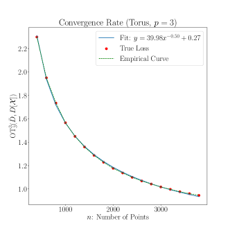
(a) The loss curve for $p=3$

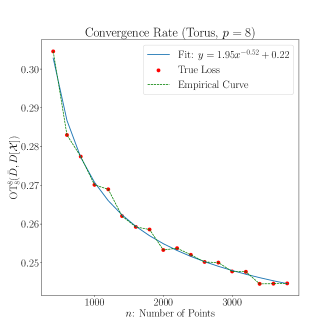
(b) The loss curve for $p=8$

Figure 1: Convergence rate verification for mean persistence measure on the Torus (point cloud of $N=50,000$ points).

Sphere.

We take $\mathcal{X}$ to be the sample set consisting of $N=20,000$ points from a 3-dimensional sphere with radius 0.5. Then we sample $B=\lfloor n^{2/3}\rfloor$ subsets each consisting of $n$ points to compute the empirical mean persistence measure. We repeat the subsampling procedure so that $n$ ranges from 600 to 4,000. In this case $b$ is assumed to be 3. If we take $p=2$, the loss curve takes the form

$$\mathbb{E}[\mathrm{OT}_{2}^{2}(\bar{D},D[\mathcal{X}])]\approx a_{0}+a_{1}n^{-\frac{1}{3}}.$$ (31)

If we take $p=9$, the bias vanishes in a rate $\beta=2$. Thus the loss curve is dominated by variance and should be in the same form as (31). We fit the loss curves using the empirical losses. The result shown in Figure 2 presents convergence rates of 0.32 and 0.36, which are consistent with our theory.

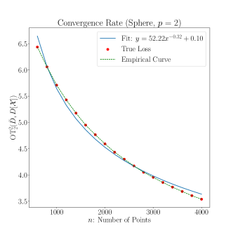
(a) The loss curve for $p=2$

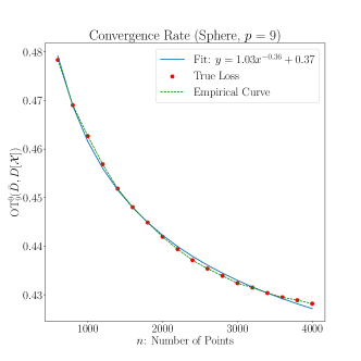
(b) The loss curve for $p=9$

Figure 2: Convergence rate verification for mean persistence measure on the Sphere (point cloud of $N=20,000$ points).

5.2 Persistence Measures vs Fréchet Means

We now provide experimental comparisons of the Fréchet mean and persistence measures as measures of central tendency in our subsampling approach on three types of data: Euclidean point clouds, abstract finite metric spaces, and networks. Although our convergence analysis assumes point cloud data in Euclidean space, these experiments demonstrate the applicability of our subsampling method to other types of data.

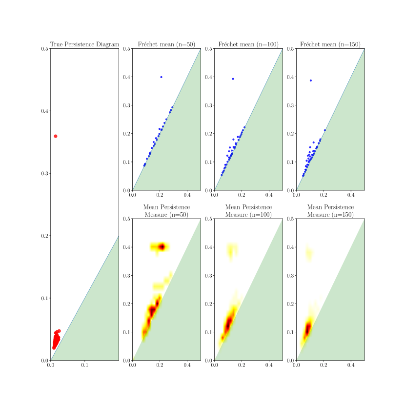
Figure 3: Illustration of Fréchet means of persistence diagrams and mean persistence measures for varying sample sizes. The left panel is the true persistence diagram of the sample set $\mathcal{X}$ computed from the Annulus. The top row shows the Fréchet mean of persistence diagrams of subsampled sets of different sizes. The bottom row shows the mean persistence measures of persistence diagrams of subsampled sets of different sizes.

Annulus.

Here we take $\mathcal{X}$ to be a sample set of $N=5,000$ points from an annulus with outer radius 0.5 and inner radius 0.2. The Fréchet mean and mean persistence measures are computed based on $B=20$ sets of subsamples from $\mathcal{X}$ each consisting of $n$ points, where $n$ ranges from 50 to 400. Figure 3 compares Fréchet mean persistence diagreams and mean persistence measures for subsets of different sizes $n$ to the true persistence diagram.

HIV Data.

We consider the HIV dataset collected by Otter et al. (2017) as the true data set $\mathcal{X}$. The HIV data set consists of 1,088 genomic sequences and the difference between any two sequences is measured by the Hamming distance. Thus, the HIV data set can be viewed as a finite metric space. We compute its persistent homology based on the VR filtration. We subsample $B=25$ subsets from $\mathcal{X}$ each consisting of $n$ points, where $n$ ranges from 100 to 300. From these subsamples we compute both the Fréchet mean and mean persistence measure.

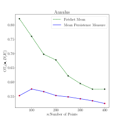
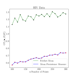
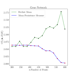
Figure 4: Comparison of Fréchet means and mean persistence measures of persistence diagrams computed from subsamples drawn from the Annulus, HIV and Gene Network data.

Gene Network.

We use a gene network from Rossi and Ahmed (2015); Cho et al. (2014) as our true data set $\mathcal{X}$. The gene network is an undirected weighted graph consisting of 924 nodes and 3,233 edges. The nodes represent genes and weights represent intensities of genetic interactions. The persistent homology is computed using the weight matrix. We subsample $B=30$ subgraphs from $\mathcal{X}$, each consisting of $n$ nodes, where $n$ ranges from 200 to 600. The persistent homology of each subgraph can be computed using the submatrix from the total weight matrix. We compute the 2-Wasserstein distances between the mean diagrams or measures and the true persistence diagram $D[\mathcal{X}]$. The loss curves are shown in Figure 4.

Robustness Comparison.

We test the robustness of the Fréchet means against the mean persistence measures in our subsampling approach by contaminating the Annulus and Gene Network with Gaussian noise. Specifically, let $W$ be the matrix consisting of points in Annulus or weights in Gene Network. We create noisy data by $\widetilde{W}=W+V$ where $V$ is a matrix of the same shape as $W$ whose elements are i.i.d. samples from the Gaussian distribution $\mathcal{N}(0,\sigma)$. We compute the mean persistence measures and Fréchet means using sample sets from the noisy data and then compute the error with respect to the true persistence diagrams of the original data sets. The loss curves are plotted in Figure 5.

These experimental results show that mean persistence measures are more accurate and more robust than Fréchet means. The reason lies in two aspects: from the theoretical perspective, the variance of Fréchet means decreases in a complicated manner due to the nonnegative curvature of $(\mathcal{D}_{2},\mathrm{W}_{2})$, while from the algorithmic prespective, the greedy algorithm returns unstable local minima which lead to fluctuating approximation errors.

The results for HIV data and Gene Network also demonstrate that subsampling and approximating the true persistence diagram by mean persistence measures also performs well on general finite metric spaces.

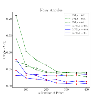
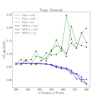
Figure 5: Robustness comparison for computed Fréchet means and mean persistence measure of persistence diagrams computed from subsamples drawn from the Annulus data and Gene Network data.

6 Applications to Real Data

Here we demonstrate our method on real-world point cloud data. We begin with examples of the computation procedure and results on large datasets, we then given an example of a real-world machine learning application of shape clustering.

6.1 Examples on Large Datasets

We study two datasets, ‘Knot’ and ‘Lock,’ obtained from a publicly available repository.

Knot.

The underlying manifold for Knot is a tubular trefoil knot. The original point cloud consists of $N=478,704$ points, which makes it impossible to compute persistent homology directly. We subsample $B=25$ subsets, each consisting of $n=9,500$ points from the original set, and compute their 1-dimensional persistence diagrams. We manually filter points with persistence less than 0.1 since the star-like ornaments on the surface will generate small noisy circles during filtration. The mean persistence measure and Fréchet mean of persistence diagrams are presented in Figure 6. From the mean persistence measure we can see three clusters of points on the half plane. The top cluster corresponds to the longest circle, i.e., the trefoil knot, while the bottom cluster corresponds to the small circle of the tube. The middle cluster represents homology classes created by self-intersections of the surface during its growth in VR filtration. The top point in Fréchet mean persistence diagram is consistent with the top cluster in mean persistence measure which indicates a longest cycle. However, we see that the Fréchet mean shows artificial homological noise near the boundary, even though each persistence diagram does not show points with small persistence.

To quantize the mean persistence measures as discussed in Section 2.4, we use the resulting computed mean persistence measure and Fréchet mean diagrams to initialize 1 centroid at $(0.05,\,0.35)$, 4 centroids around $(0.07,\,0.2)$ and 2 centroids around $(0.04,\,0.1)$, and then apply the quantization algorithm in Divol and Lacombe (2021); Chazal et al. (2021). Figure 6(d) shows the quantized persistence diagram of the mean persistence measure.

(a) Original data

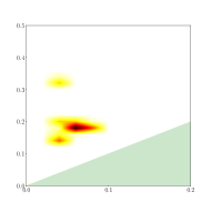
(b) Mean persistence measure

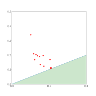
(c) Fréchet mean

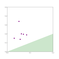
(d) Quantization of (b)

Figure 6: Approximation of the persistent homology of Knot. (a) Original point cloud with $N=478,704$ points; (b) Mean persistence measure for dimension 1 homology for one subsample of $n=9,500$ points; (c) Fréchet mean for dimension 1 homology for one subsample of $n=9,500$ points; (d) Quantization of the mean persistence measure shown in (b). In (b), the bottom cluster shows the small circle of the tube, while the middle cluster in the mean persistence measure indicates homology classes generated by intersections of the surfaces during VR filtration. In (c), the topmost point in the Fréchet mean represents the homology of the trefoil knot, which is also presented by the top yellow cluster in (b).

Lock.

The point cloud is roughly composed of three parts, with one tube in the center and two caps on two sides. Each cap can be viewed as a closed surface of genus 4. Thus the underlying manifold for Lock is homeomorphic to the connected sum of a torus and two surfaces of genus 4, which is essentially a closed surface of genus 9. The original point cloud consists of $N=460,592$ points, which again is too large to compute persistent homology on directly. We subsample $B=30$ subsets, each consisting of $n=9,000$ points from the original set and compute their 1-dimensional persistence diagrams. The mean persistence measure and Fréchet mean of persistence diagrams are presented in Figure 7. From the Fréchet mean persistence diagram we can easily see the point with the largest persistence. This point corresponds to the largest circle in the central tube. Right below the top point there are 8 points corresponding to 8 circles which bound holes on the caps. In theory, there should be 18 circles generating the 1-dimensional homology of the underlying manifold. However, the remaining 9 circles are of small radii and are mixed up with noisy circles generated by VR filtration. The middle cluster and bottom cluster in the mean persistence measure are consistent with results shown in Fréchet mean. The only difference is that the top cluster is not obvious (in very shallow yellow). This is a matter of visualization as there is only one point at the top in each persistence diagram and they cannot concentrate as a cluster compared to other group of points.

As above, based on the observations from mean persistence measure and Fréchet mean, we initialize 1 centroid at $(0.05,\,0.3)$, 8 centroids around $(0.05,\,0.2)$ and 9 centroids around $(0.05,\,0.1)$, and then apply the quantization algorithm. Figure 7(d) shows the quantized persistence diagram from the mean persistence measure, which can be regarded as a faithful representative of the persistent homology of the original data.

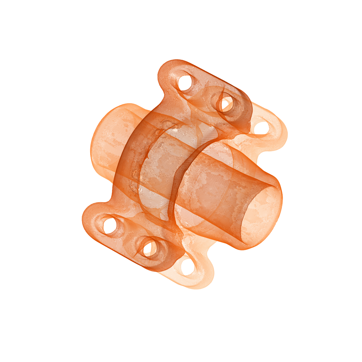
(a) Original data

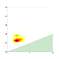
(b) Mean persistence measure

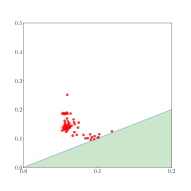
(c) Fréchet mean

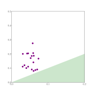
(d) Quantization of (b)

Figure 7: Approximation of the persistent homology of Lock. (a) Original point cloud with $N=460,592$ points; (b) Mean persistence measure for dimension 1 homology computed from one subsample of $n=9,000$ points; (c) Fréchet mean for dimension 1 homology computed from one subsample of $n=9,000$ points; (d) Quantization of the mean persistence measure shown in (b). In (b), there are two clear clusters and a cluster at the top in very shallow yellow. Combined with (c), the point with largest persistence (with respect to the top cluster in shallow yellow) corresponds to the largest circle in the central tube, while the points with $y$-coordinate close to 0.2 (with respect the middle cluster) correspond to 8 circles bounding the holes on two caps, the remaining points (with respect the bottom cluster) correspond to small circles together with some topological noise generated by the VR filtration.

From these two real data examples we can see both merits and limitations of both the mean persistence measure and Fréchet mean as representatives of central tendency for persistence diagrams computed from subsampled data: the clusters (concentrations of measures) in mean persistence measures indicate partial locations of the persistent homology of the original data. However, we cannot read the actual number of points as mean persistence measures are not diagrams. In addition, points with large persistence may not group as clusters, which makes them difficult to visualize. In contrast, Fréchet means are diagrams so we can read the multiplicity of points, and points with large persistence are easy to visualize. However, Fréchet means can generate artificial noise, which can mix up with other points and affect the identification of “true” persistent homology. To bypass the difficulty of interpretation for mean persistence measures, quantization may be applied to obtain a representative persistence diagram from mean persistence measures, with the results from the computed Fréchet mean to drive the initialization procedure.

6.2 A Real-World Application: Shape Clustering

We now use the mean persistence measure and Fréchet mean of persistence diagrams in a machine learning task of shape clustering on real-world data. The Mechanical Components Benchmark (MCB) is a large-scale dataset of 3D objects of mechanical components collected from online 3D computer aided design (CAD) repositories (Kim et al., 2020). MCB has 18,038 point cloud datasets with 25 classes. The size of each point cloud has a wide range from hundreds to millions of points. The quality of each point cloud also varies, as some point clouds do not present a clear shape. We extract point clouds from two classes: ‘Bearing’ and ‘Motor.’ We discarded datasets with extremely small and large numbers of points. After this pre-selection, we obtain 74 sets from Bearing and 53 sets from Motor. Each dataset consists of a range from $N=30,000$ to $N=250,000$ points. Figure 8 shows some examples from two classes.

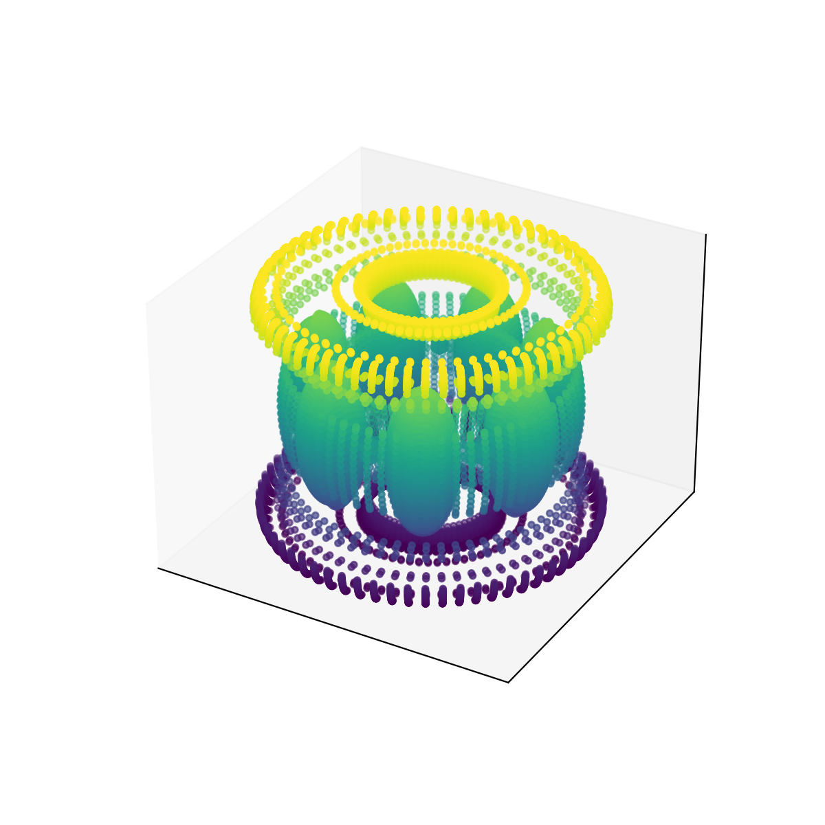
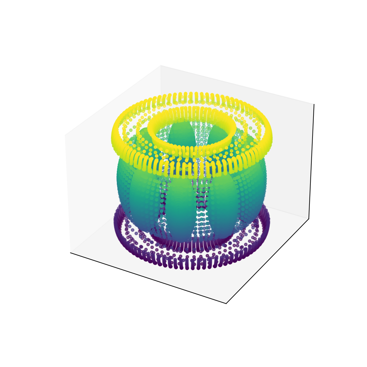
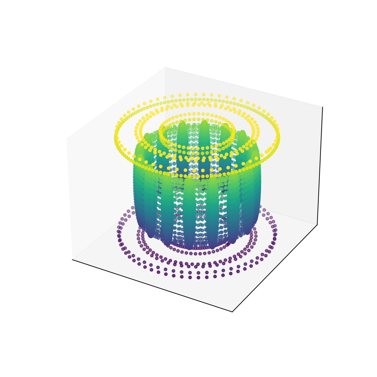
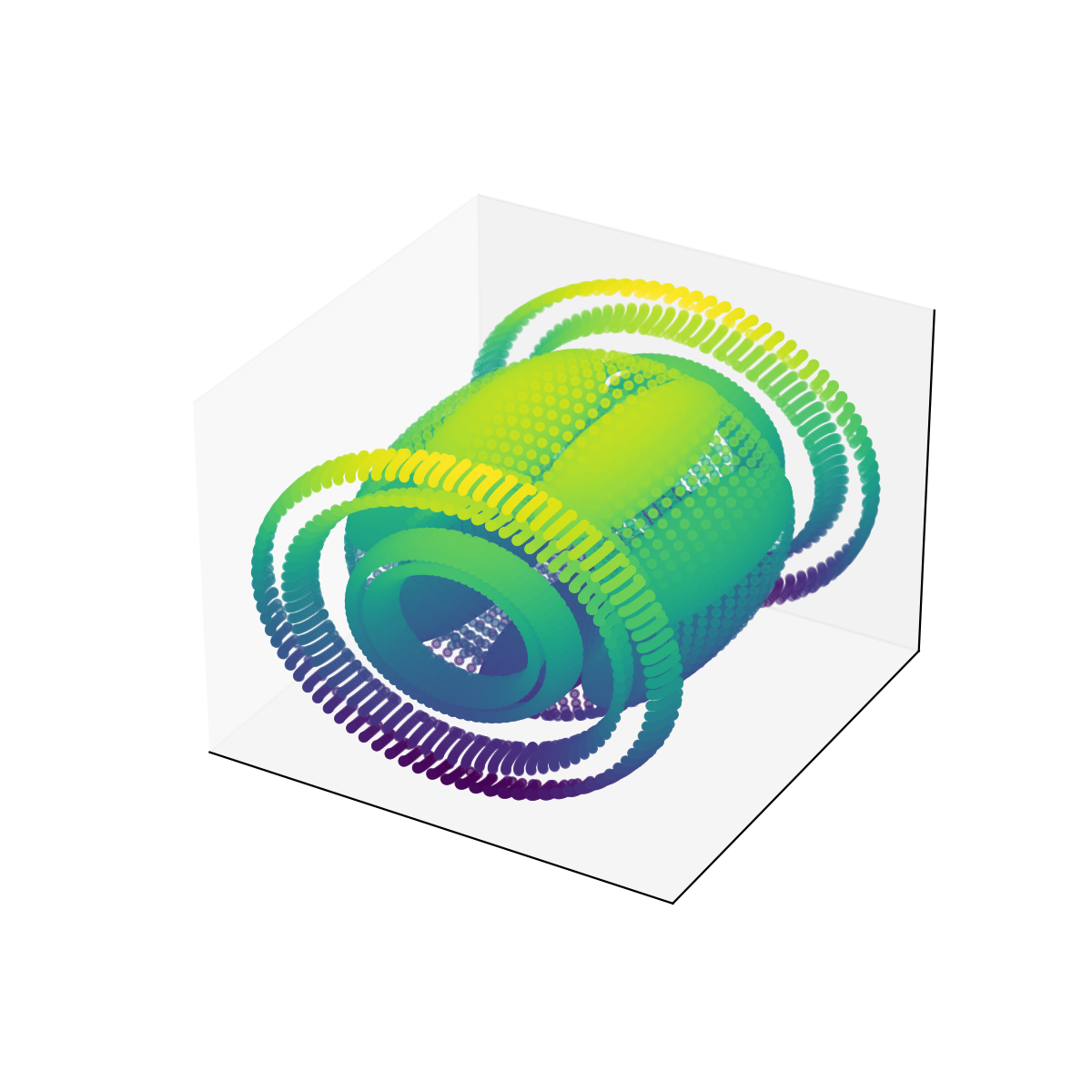
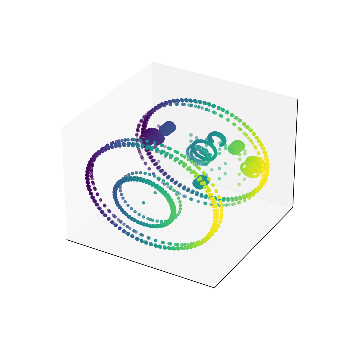
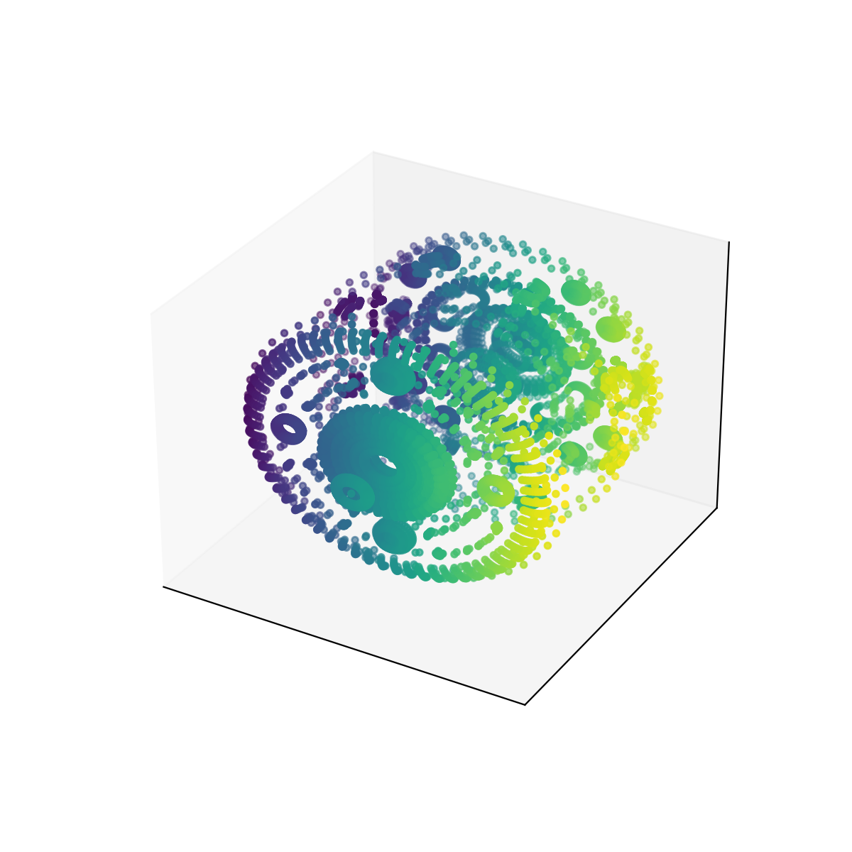
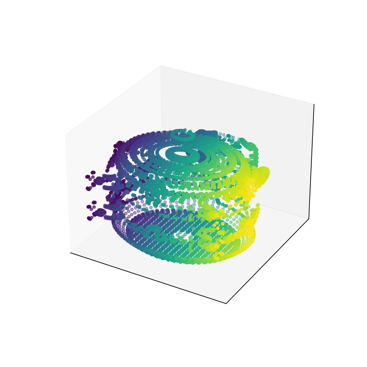
Figure 8: Some example point clouds from Bearing and Motor. The first row presents sets from Bearing and the second from Motor.

Given the 127 point clouds, we would like to classify them into two clusters—representing Bearing and Motor, respectively—using persistent homology. Note that a direct computation of persistent homology is not feasible, as most point clouds are massive. Therefore, we approximate their persistent homology using mean persistence measures and Fréchet means computed from subsampled sets. For each point cloud, we subsample $B=15$ sets, each consisting of 2% number of points of the original data set. Then we compute the mean persistence measure and Fréchet mean as discussed above. In both computations, we compute the mutual $\mathrm{OT}_{2}$ distance, which is stored as distance matrix and then used as the input of UMAP for dimension reduction (McInnes et al., 2018). The 127 point clouds are embedded into the 2D plane by UMAP. The results after dimension reduction are shown in Figure 9, where points are colored according to their true labels. We then use DBSCAN to classify these points into two clusters (Ester et al., 1996). As shown in Figure 9, the two clusters are close to the true labels.

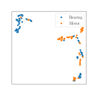
(a) UMAP for mean persistence measures

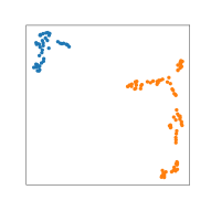
(b) DBSCAN for mean persistence measures

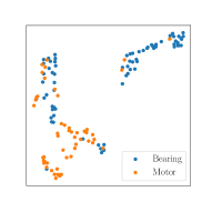
(c) UMAP for Fréchet means

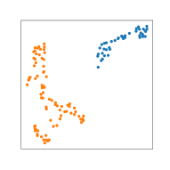
(d) DBSCAN for Fréchet means

Figure 9: Dimension reduction using UMAP and clustering using DBSCAN.

Data and Software Availability

Data.

The point cloud imaging datasets ‘Knot’ and ‘Lock’ were obtained from the shape repository Digital Shape Workbench (http://visionair.ge.imati.cnr.it/). ‘Bearing’ and ‘Motor’ were obtained from the Mechanical Components Benchmark (Kim et al., 2020).

Software.

The computation of persistent homology is implemented using GUDHI and Giotto-tda (The GUDHI Project, 2022; Tauzin et al., 2021). The computation of optimal transport is implemented using POT (Flamary et al., 2021). The code for all numerical experiments in this paper can be found at https://github.com/YueqiCao/PD-subsample.

7 Discussion

In this work, we provided a practical workaround to the problem of prohibitive computational expenses in persistent homology. For datasets that are simply too large to compute persistent homology, we have shown that the mean of persistence diagrams computed from multiple smaller subsamples of the large dataset provides a good approximation for the true persistent homology of the large dataset. Specifically, we have shown that the mean persistence measure accurately estimates the persistence diagram of the original massive dataset. Furthermore, under certain assumptions, we gave the finite sample convergence rate of the mean persistence diagram (as a mean persistence measure) under optimal partial transport distance, and verified it with synthetic experiments. We demonstrated the practical performance of mean persistence measures and Fréchet means on a variety of real datasets and data types.

Our work inspires several future directions of research, which we now list.

Variance estimation for Fréchet means. Currently there exists no convergence rate estimation of variance for Fréchet means. Le Gouic et al. (2019) proposed a geometric condition for the fast convergence of empirical Fréchet means in Alexandrov spaces of nonnegative curvature, which may be a starting point to study the convergence and derive corresponding variance rates, for example, on $(\mathcal{D}_{2},\mathrm{W}_{2})$ which is known to be a nonnegative curved Alexandrov space (Turner et al., 2014).

Combining mean persistence measures and Fréchet means. In the application real large point cloud data in Sections 5.2 and 6.1, we saw that mean persistence measure and Fréchet means both have merits and drawbacks, and in some sense, they compensate each other. An interesting possibility would be to construct a new representation of persistent homology that combines the advantages of both methods.

Subsampling for other data types. In this work, we have derived theoretical results of subsampling methods under the assumption that the input data takes the form of Euclidean point clouds. In practice subsampling methods may also be adapted to other data types. As we have seen experimentally in Section 5.2, our proposed subsampling approach also performs well for general finite metric spaces and weighted graphs. An open direction of research is to derive similar convergence analysis results to what we have found and determine whether our results can be generalized to finite metric spaces and graphs. Additionally, from the practical perspective, it would also be worthwhile to explore other types of data such as images and explore the general applicability of subsampling and computing persistent homology in these settings.

Subsampling for continuous spaces. In this paper we always assume that the total space $\mathcal{X}$ is a finite space. This assumption is critical for our analysis since the Wasserstein stability result of Skraba and Turner (2020) only holds when the number of point clouds has a uniform bound. An important generalization would be to extend the subsampling method to cases where $\mathcal{X}$ is any compact metric space.

Applications to machine learning. Persistent homology has been applied in many machine learning settings, including as graph neural networks (Zhao et al., 2020), graph classification (Carrière et al., 2020), and deep neural networks (Rieck et al., 2018). An interesting direction of study would be to determine how to use subsampling methods may be used to enhance the training and construction of neural networks.

References

- Adams and Carlsson (2015) Adams, H. and G. Carlsson (2015). Evasion paths in mobile sensor networks. The International Journal of Robotics Research 34(1), 90–104.
- Anderson et al. (2018) Anderson, K. L., J. S. Anderson, S. Palande, and B. Wang (2018). Topological data analysis of functional MRI connectivity in time and space domains. In International Workshop on Connectomics in Neuroimaging, pp. 67–77. Springer.
- Bauer and Lesnick (2020) Bauer, U. and M. Lesnick (2020). Persistence diagrams as diagrams: A categorification of the stability theorem. In Topological Data Analysis, pp. 67–96.
- Betthauser et al. (2022) Betthauser, L., P. Bubenik, and P. B. Edwards (2022). Graded persistence diagrams and persistence landscapes. Discrete & Computational Geometry 67(1), 203–230.
- Botnan and Lesnick (2018) Botnan, M. and M. Lesnick (2018). Algebraic stability of zigzag persistence modules. Algebraic & geometric topology 18(6), 3133–3204.
- Bubenik (2015a) Bubenik, P. (2015a). Statistical topological data analysis using persistence landscapes. Journal of Machine Learning Research 16(1), 77–102.
- Bubenik (2015b) Bubenik, P. (2015b). Statistical topological data analysis using persistence landscapes. Journal of Machine Learning Research 16, 77–102.
- Bubenik (2020) Bubenik, P. (2020). The persistence landscape and some of its properties. In Topological Data Analysis, pp. 97–117.
- Bubenik et al. (2018) Bubenik, P., J. Scott, and D. Stanley (2018). An algebraic Wasserstein distance for generalized persistence modules. arXiv preprint arXiv:1809.09654.
- Bubenik and Scott (2014) Bubenik, P. and J. A. Scott (2014). Categorification of persistent homology. Discrete & Computational Geometry 51(3), 600–627.
- Carrière et al. (2020) Carrière, M., F. Chazal, Y. Ike, T. Lacombe, M. Royer, and Y. Umeda (2020). Perslay: A neural network layer for persistence diagrams and new graph topological signatures. In International Conference on Artificial Intelligence and Statistics, pp. 2786–2796. PMLR.
- Chazal et al. (2009) Chazal, F., D. Cohen-Steiner, M. Glisse, L. J. Guibas, and S. Y. Oudot (2009). Proximity of persistence modules and their diagrams. In Proceedings of the twenty-fifth annual symposium on Computational geometry, pp. 237–246.
- Chazal et al. (2009) Chazal, F., D. Cohen-Steiner, L. J. Guibas, F. Mémoli, and S. Y. Oudot (2009). Gromov–Hausdorff stable signatures for shapes using persistence. In Computer Graphics Forum, Volume 28, pp. 1393–1403. Wiley Online Library.
- Chazal et al. (2016) Chazal, F., V. De Silva, M. Glisse, and S. Oudot (2016). The structure and stability of persistence modules.
- Chazal et al. (2015) Chazal, F., B. Fasy, F. Lecci, B. Michel, A. Rinaldo, and L. Wasserman (2015). Subsampling methods for persistent homology. In International Conference on Machine Learning, pp. 2143–2151. PMLR.
- Chazal et al. (2015) Chazal, F., B. T. Fasy, F. Lecci, A. Rinaldo, and L. Wasserman (2015). Stochastic convergence of persistence landscapes and silhouettes. Journal of Computational Geometry 6(2), 140–161.
- Chazal et al. (2014) Chazal, F., M. Glisse, C. Labruère, and B. Michel (2014). Convergence rates for persistence diagram estimation in topological data analysis. In International Conference on Machine Learning, pp. 163–171. PMLR.
- Chazal et al. (2020) Chazal, F., C. Levrard, and M. Royer (2020). Optimal quantization of the mean measure and application to clustering of measures. arXiv preprint arXiv:2002.01216.
- Chazal et al. (2021) Chazal, F., C. Levrard, and M. Royer (2021). Clustering of measures via mean measure quantization. Electronic Journal of Statistics 15(1), 2060 – 2104.
- Cho et al. (2014) Cho, A., J. Shin, S. Hwang, C. Kim, H. Shim, H. Kim, H. Kim, and I. Lee (2014). WormNet v3: a network-assisted hypothesis-generating server for Caenorhabditis elegans. Nucleic acids research 42(W1), W76–W82.
- Cohen-Steiner et al. (2007) Cohen-Steiner, D., H. Edelsbrunner, and J. Harer (2007). Stability of persistence diagrams. Discrete & computational geometry 37(1), 103–120.
- Cohen-Steiner et al. (2010) Cohen-Steiner, D., H. Edelsbrunner, J. Harer, and Y. Mileyko (2010). Lipschitz functions have -stable persistence. Foundations of computational mathematics 10(2), 127–139.
- Crawford et al. (2020) Crawford, L., A. Monod, A. X. Chen, S. Mukherjee, and R. Rabadán (2020). Predicting Clinical Outcomes in Glioblastoma: An Application of Topological and Functional Data Analysis. Journal of the American Statistical Association 115(531), 1139–1150.
- Cuevas (2009) Cuevas, A. (2009, 01). Set estimation: Another bridge between statistics and geometry. Boletín de Estadística e Investigación Operativa 25(2), 71–85.
- Cuevas and Rodríguez-Casal (2004) Cuevas, A. and A. Rodríguez-Casal (2004). On boundary estimation. 36(2), 340–354. Publisher: Cambridge University Press.
- Divol and Chazal (2019) Divol, V. and F. Chazal (2019). The density of expected persistence diagrams and its kernel based estimation. Journal of Computational Geometry 10(2), 127–153.
- Divol and Lacombe (2019) Divol, V. and T. Lacombe (2019). Understanding the topology and the geometry of the persistence diagram space via optimal partial transport. arXiv preprint arXiv:1901.03048.
- Divol and Lacombe (2021) Divol, V. and T. Lacombe (2021). Estimation and quantization of expected persistence diagrams. arXiv preprint arXiv:2105.04852.
- Edelsbrunner et al. (2000) Edelsbrunner, H., D. Letscher, and A. Zomorodian (2000). Topological persistence and simplification. In Proceedings 41st Annual Symposium on Foundations of Computer Science, pp. 454–463.
- Ester et al. (1996) Ester, M., H.-P. Kriegel, J. Sander, X. Xu, et al. (1996). A density-based algorithm for discovering clusters in large spatial databases with noise. In kdd, Volume 96, pp. 226–231.
- Fasy et al. (2014) Fasy, B. T., F. Lecci, A. Rinaldo, L. Wasserman, S. Balakrishnan, and A. Singh (2014). Confidence sets for persistence diagrams. The Annals of Statistics 42(6), 2301–2339.
- Flamary et al. (2021) Flamary, R., N. Courty, A. Gramfort, M. Z. Alaya, A. Boisbunon, S. Chambon, L. Chapel, A. Corenflos, K. Fatras, N. Fournier, L. Gautheron, N. T. Gayraud, H. Janati, A. Rakotomamonjy, I. Redko, A. Rolet, A. Schutz, V. Seguy, D. J. Sutherland, R. Tavenard, A. Tong, and T. Vayer (2021). Pot: Python optimal transport. Journal of Machine Learning Research 22(78), 1–8.
- Frosini and Landi (1999) Frosini, P. and C. Landi (1999). Size theory as a topological tool for computer vision. Pattern Recognition and Image Analysis 9(4), 596–603.
- Hille et al. (2021) Hille, S. C., T. Szarek, D. T. Worm, and M. A. Ziemlańska (2021). Equivalence of equicontinuity concepts for Markov operators derived from a Schur-like property for spaces of measures. Statistics & Probability Letters 169, 108964.
- Hiraoka et al. (2018) Hiraoka, Y., T. Shirai, and K. D. Trinh (2018). Limit theorems for persistence diagrams. The Annals of Applied Probability 28(5), 2740–2780.
- Hirata et al. (2020) Hirata, A., T. Wada, I. Obayashi, and Y. Hiraoka (2020). Structural changes during glass formation extracted by computational homology with machine learning. Communications Materials 1(1), 1–8.
- Kim et al. (2020) Kim, S., H.-g. Chi, X. Hu, Q. Huang, and K. Ramani (2020). A large-scale annotated mechanical components benchmark for classification and retrieval tasks with deep neural networks. In Proceedings of 16th European Conference on Computer Vision (ECCV).
- Lacombe et al. (2018) Lacombe, T., M. Cuturi, and S. Oudot (2018). Large scale computation of means and clusters for persistence diagrams using optimal transport. Advances in Neural Information Processing Systems 31.
- Le Gouic et al. (2019) Le Gouic, T., Q. Paris, P. Rigollet, and A. J. Stromme (2019). Fast convergence of empirical barycenters in Alexandrov spaces and the Wasserstein space. arXiv preprint arXiv:1908.00828.
- Lesnick (2015) Lesnick, M. (2015). The theory of the interleaving distance on multidimensional persistence modules. Foundations of Computational Mathematics 15(3), 613–650.
- McInnes et al. (2018) McInnes, L., J. Healy, N. Saul, and L. Grossberger (2018). UMAP: Uniform manifold approximation and projection. The Journal of Open Source Software 3(29), 861.
- Mileyko et al. (2011) Mileyko, Y., S. Mukherjee, and J. Harer (2011). Probability measures on the space of persistence diagrams. Inverse Problems 27(12), 124007.
- Nonnenmacher et al. (1995) Nonnenmacher, D., R. Zagst, et al. (1995). A new form of Jensen’s inequality and its application to statistical experiments. Journal of the Australian Mathematical Society, Series B 36(4), 389–398.
- Ohta (2012) Ohta, S.-i. (2012). Barycenters in alexandrov spaces of curvature bounded below. Advances in geometry 12(4), 571–587.
- Otter et al. (2017) Otter, N., M. A. Porter, U. Tillmann, P. Grindrod, and H. A. Harrington (2017). A roadmap for the computation of persistent homology. EPJ Data Science 6, 1–38.
- Reani and Bobrowski (2021) Reani, Y. and O. Bobrowski (2021). Cycle registration in persistent homology with applications in topological bootstrap. arXiv preprint arXiv:2101.00698.
- Rieck et al. (2018) Rieck, B., M. Togninalli, C. Bock, M. Moor, M. Horn, T. Gumbsch, and K. Borgwardt (2018). Neural persistence: A complexity measure for deep neural networks using algebraic topology. In International Conference on Learning Representations.
- Rossi and Ahmed (2015) Rossi, R. and N. Ahmed (2015). The network data repository with interactive graph analytics and visualization. In Twenty-ninth AAAI conference on artificial intelligence.
- Skraba and Turner (2020) Skraba, P. and K. Turner (2020). Wasserstein stability for persistence diagrams. arXiv preprint arXiv:2006.16824.
- Solomon et al. (2021) Solomon, E., A. Wagner, and P. Bendich (2021). From Geometry to Topology: Inverse Theorems for Distributed Persistence. arXiv:2101.12288.
- Tauzin et al. (2021) Tauzin, G., U. Lupo, L. Tunstall, J. B. Pérez, M. Caorsi, A. M. Medina-Mardones, A. Dassatti, and K. Hess (2021). giotto-tda:: A topological data analysis toolkit for machine learning and data exploration. J. Mach. Learn. Res. 22, 39–1.
- The GUDHI Project (2022) The GUDHI Project (2022). GUDHI User and Reference Manual (3.5.0 ed.).
- Turner (2013) Turner, K. (2013). Means and medians of sets of persistence diagrams. arXiv preprint arXiv:1307.8300.
- Turner et al. (2014) Turner, K., Y. Mileyko, S. Mukherjee, and J. Harer (2014). Fréchet means for distributions of persistence diagrams. Discrete & Computational Geometry 52(1), 44–70.
- Vlontzos et al. (2021) Vlontzos, A., Y. Cao, L. Schmidtke, B. Kainz, and A. Monod (2021). Topological data analysis of database representations for information retrieval. arXiv:2104.01672.
- Zhao et al. (2020) Zhao, Q., Z. Ye, C. Chen, and Y. Wang (2020). Persistence enhanced graph neural network. In International Conference on Artificial Intelligence and Statistics, pp. 2896–2906. PMLR.
- Zomorodian and Carlsson (2005) Zomorodian, A. and G. Carlsson (2005). Computing persistent homology. Discrete & Computational Geometry 33(2), 249–274.