OSSOS XXV: Large Populations and Scattering-Sticking in the Distant Transneptunian Resonances

Abstract

There have been 77 TNOs discovered to be librating in the distant transneptunian resonances (beyond the 2:1 resonance, at semimajor axes greater than 47.7 AU) in four well-characterized surveys: the Outer Solar System Origins Survey (OSSOS) and three similar prior surveys. Here we use the OSSOS Survey Simulator to measure their intrinsic orbital distributions using an empirical parameterized model. Because many of the resonances had only one or very few detections, $j$:$k$ resonant objects were grouped by $k$ in order to have a better basis for comparison between models and reality. We also use the Survey Simulator to constrain their absolute populations, finding that they are much larger than predicted by any published Neptune migration model to date; we also find population ratios that are inconsistent with published models, presenting a challenge for future Kuiper Belt emplacement models. The estimated population ratios between these resonances are largely consistent with scattering-sticking predictions, though further discoveries of resonant TNOs with high-precision orbits will be needed to determine whether scattering-sticking can explain the entire distant resonant population or not.

1 Introduction

Observations of the outer solar system indicate an enormous number of objects trapped within the very distant mean-motion resonances with Neptune. This work aims to provide a greater understanding of the absolute populations in these different resonances, the distribution of orbital elements within each resonance, as well as to help identify the primary mechanism by which these distant resonances are populated. Population of these distant resonances may occur through sweep-up during a smooth phase of Neptune’s migration (e.g. Hahn & Malhotra, 2005), during circularization of Neptune’s orbit after a Nice Model-style instability (e.g. Levison et al., 2008), or may be primarily populated by “scattering-sticking”: unstable scattering TNOs temporarily sticking within resonances (e.g. Yu et al., 2018).

Previous papers (e.g., Gladman et al., 2012; Pike et al., 2015; Alexandersen et al., 2016; Volk et al., 2016, 2018; Chen et al., 2019) have already modelled many of the resonant populations in detail, however, all of the distant high-order resonant populations have not yet been modelled. This paper shall refer to all resonances beyond the 2:1 resonance at 47.7 AU as ‘distant’ resonances.

Several of the distant resonances between 2:1 and 5:1 were modelled by Gladman et al. (2012), who measured large population estimates. Individual analyses of the 3:1 (Alexandersen et al., 2016), 4:1 (Lawler, 2013; Alexandersen et al., 2016), 5:1 (Pike et al., 2015), and 9:1 (Volk et al., 2018) have also been carried out. However, these are only a few of the many resonances for which we have detections and thus modelling capability.

Previous theoretical works suggest mechanisms which could have built up the resonant populations within the distant Solar System. Kaib & Sheppard (2016) state that resonant objects beyond the 4:1 resonance are less strongly affected by Neptune’s migration due to Kozai cycling timescales. Furthermore, Pike et al. (2015); Volk et al. (2018) both found that the large libration amplitudes of the small number of discovered 5:1 and 9:1 resonators were consistent with scattering-sticking, but the absolute population implied by the observed TNOs was larger than could be easily explained by scattering-sticking. These previous results point to distant resonances being populated by TNOs from the scattering population sticking to resonances rather than being swept up during Neptune’s migration itself, although whether the relative population sizes within resonances supports this theory remains unclear.

Yu et al. (2018) extensively modelled the temporary sticking of scattering TNOs within the region $a$=30-100 AU, with orbital distributions of initial populations based off the Kaib et al. (2011) scattering model and constraints on the current total population of scattering objects (Lawler et al., 2018a). After measuring the time-averaged population over 1 Gyr, they found that, at any time, approximately 40% of all objects within this semi-major axis range should be stuck in a resonance. Their simulations imply that a) approximately 1.3 times as many non-resonant scattering TNOs exist as those transiently stuck, b) a quarter of those that are stuck should exist in the $n:1$ resonances, and c) that the resonant-sticking populations should increase with semi-major axis (well demonstrated in Volk et al., 2018).

In this work, we create empirical parametric models which reproduce the observed orbits of the distant, high-order resonances in the transneptunian belt. The properties of objects within these resonances have generally not previously been measured due to the extreme difficulty of observing these distant bodies, measuring their orbits to high enough precision for resonant identification, and accounting for the complex observation biases. The rate and mode by which Neptune migrated outwards, combined with ongoing resonant sticking by the scattering population (see, e.g., Lykawka & Mukai, 2007; Yu et al., 2018), affects the distribution of objects among the different resonances that we observe today, although the relative importance of each type of emplacement, particularly for the distant resonances, is as yet unmeasured. N-body simulations show that the distribution of TNOs in resonances is different depending on which type of migration Neptune experiences (e.g. Hahn & Malhotra, 2005; Levison et al., 2008; Nesvornỳ & Vokrouhlickỳ, 2016; Kaib & Sheppard, 2016). When the final test particles are dynamically classified (as in e.g. Pike et al., 2017; Lawler et al., 2019), these models can be tested by comparison to observations from well-calibrated surveys (as in e.g. Gladman et al., 2012).

We make use of precise orbital measurements of transneptunian objects (TNOs) from the Outer Solar System Origins Survey (OSSOS; Bannister et al., 2018) in combination with three other well-characterized surveys: the Canada France Ecliptic Plane Survey (CFEPS; Petit et al., 2011), the CFEPS High Latitude Survey (HiLat; Petit et al., 2017) and the Alexandersen et al. (2016) survey. These four surveys together will be referred to as OSSOS++. We call these surveys “well-characterized” because all biases in pointing direction, magnitude limits, detection, and tracking are well-known and can be incorporated into a Survey Simulator (Lawler et al., 2018b; Petit et al., 2018). We use the Survey Simulator to subject orbital models to the same biases as the observations, allowing for robust comparisons between simulated and real detections to test the models.

In this paper, we produce a set of parameterized orbital distributions which are statistically consistent with our well-characterized distant resonant TNO observations (Sections 2 and 3). We then compare our measured populations with previously published N-body simulations of the Kuiper Belt, finding that none reproduce the quantity calculated in the following population models (Section 4). Future Solar System dynamical models must match our population models constrained by observations within their uncertainty, and this will help determine the most likely mechanism which emplaced TNOs into the distant Neptune resonances.

2 Measuring Orbital Distributions and Populations

An object is said to be in a mean-motion resonance with Neptune when its orbital period around the Sun can be written as a ratio of relatively small integers relative to Neptune’s orbital period and the repeating perturbations on the object’s orbit by Neptune causes the object to librate around the exact resonant orbit. For example, Pluto is in the 3:2 resonance with Neptune; Pluto goes around the Sun twice in the same amount of time it takes Neptune to go around the Sun three times, and the two perihelion passages Pluto makes during this resonant cycle librate around points $90^{\circ}$ to either side of Neptune. This is a simplified description of the complex phenomena that can occur in Neptune’s resonances (which include higher-order sub-resonances within these mean-motion resonances), but in general, an object in an exact $j$:$k$ external resonance with Neptune will come to perihelion at $k$ different locations relative to Neptune during each resonance cycle, as illustrated in the top panels of Figure 1. In reality, a resonant object will librate around these $k$ points, somewhat smearing out these perihelion locations in a population of resonant objects (bottom panels of Figure 1). TNOs on unstable, scattering orbits can “stick” to resonances temporarily; objects experiencing even quite distant encounters with Neptune can experience changes in semimajor axis that place them into temporarily resonant configurations with the planet. Neptune can then provide the necessary gravitational nudges to hold the TNO in the resonant orbit for anywhere from thousands to hundreds of millions of years before the TNO finally leaves the resonance and returns to an unstable scattering orbit (see Yu et al., 2018, for more a detailed discussion).

For an integer orbital period ratio $j$:$k$, we identify resonant behavior by examining the resonant angle

$$\phi_{jk}=j\lambda_{\rm TNO}-k\lambda_{\rm N}-(j-k)\varpi_{\rm TNO},$$ (1)

which for resonant objects must be confined and thus not take on all values between $0^{\circ}-360^{\circ}$; this confinement is directly related to the libration around the equilibrium points described above. In Equation 1, the mean longitude $\lambda=\Omega+\omega+\mathcal{M}$ is the combination of the orbital angles of the longitude of ascending node $\Omega$, the argument of pericenter $\omega$, and the mean anomaly $\mathcal{M}$; the longitude of pericenter $\varpi=\Omega+\omega$, and the subscripts N and TNO refer to Neptune and the TNO respectively. In principle, resonant arguments involving combinations of $\varpi_{\rm TNO}$ and $\Omega_{\rm TNO}$ are possible for each $j$:$k$ resonance. However, these distant resonant TNOs typically have high eccentricities and so the combination of arguments in equation 1 is strongest (e.g., Murray & Dermott, 2000), and we use this equation for our resonant modelling.

This confinement of orbital angles has a powerful effect on the observability of resonant TNOs: the confinement of $\phi_{jk}$ means that resonant TNOs will have their pericenters occur preferentially at set locations on the sky relative to Neptune (for a detailed example, see Lawler & Gladman, 2013). In the frame of reference that is co-rotating with Neptune, the orbits of resonant objects look like a child’s spirograph, mainly circular but with small loops at pericenter (top portion of Figure 1 shows toy models of the 7:2, 11:4, and 12:7 resonances that demonstrate this). Because surveys are most sensitive to TNOs at perihelion (as they are then closest to the Sun and thus brightest) , and different resonances have concentrations of perihelia at different sky locations, the sensitivity of a given survey to resonant TNOs can only be evaluated by including the on-sky pointings and completeness functions of the survey in careful modelling.

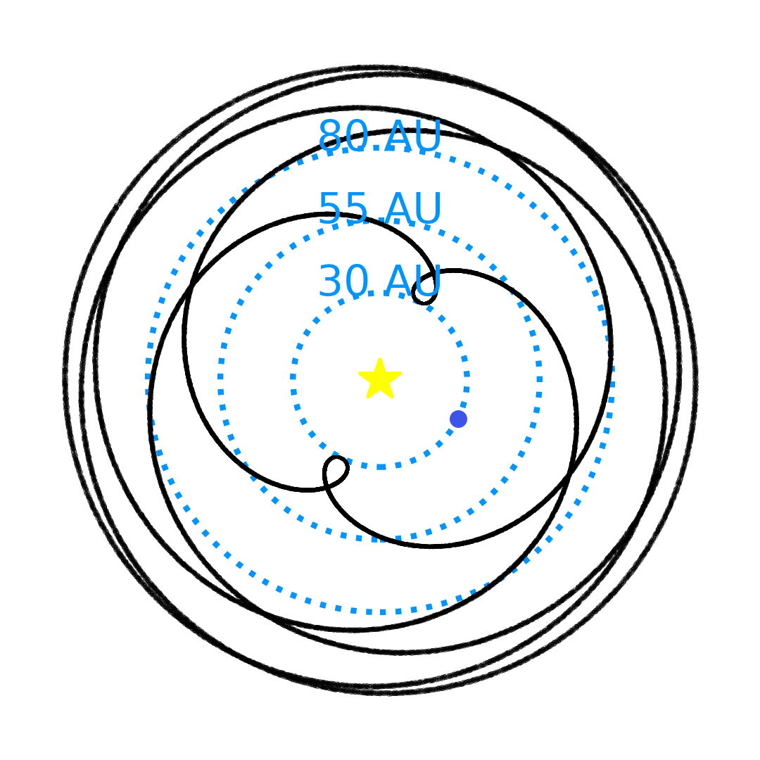
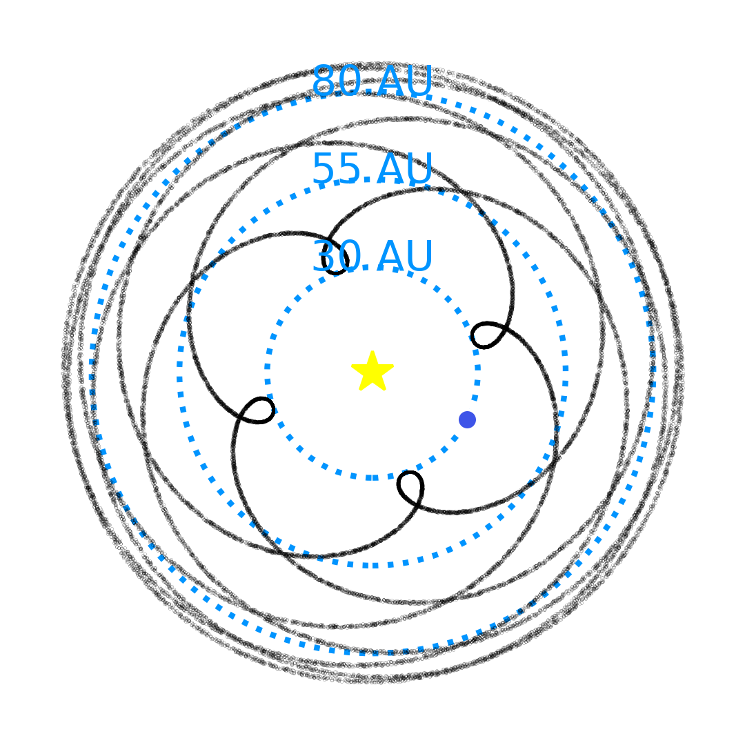
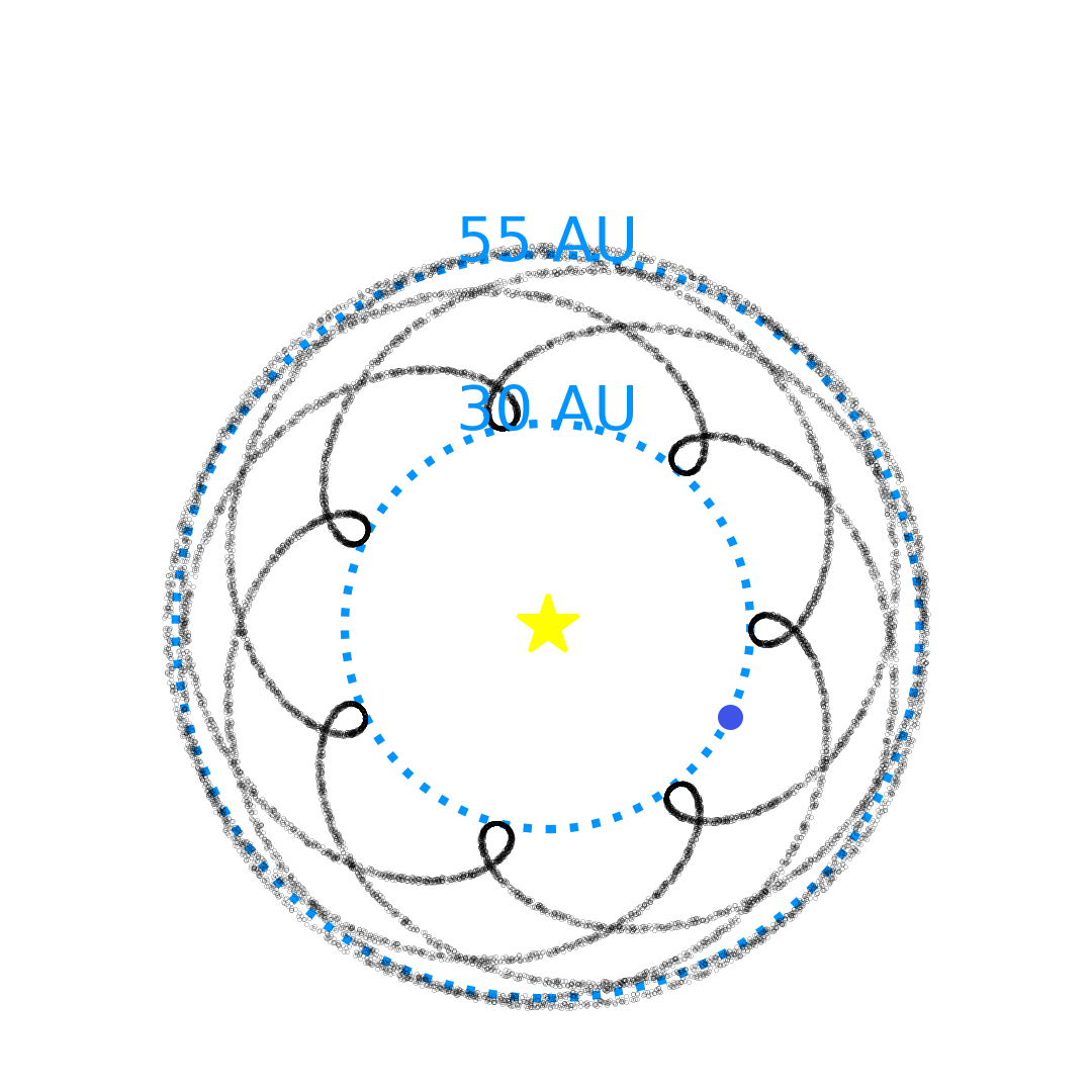
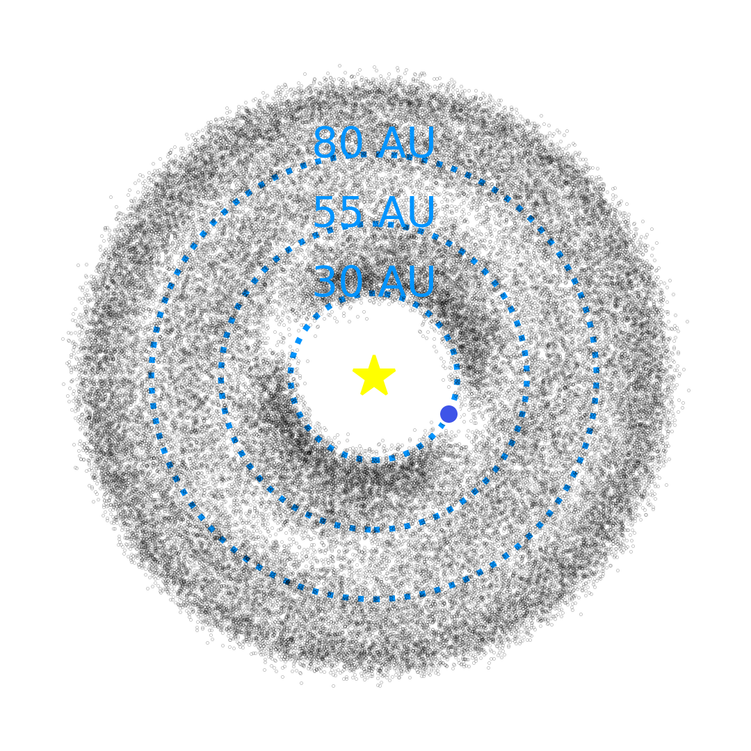
Figure 1: Top 3 panels: Toy models of 7:2 ($a=69~{}$AU), 11:4 ($a=59$ AU), and 12:7 ($a=43$ AU) resonances demonstrate the equilibrium configurations of the resonances with respect to Neptune (blue point). Bottom 3 panels: the 7:2, 11:4, and 12:7 resonances with realistic orbital distributions, where libration amplitude can be large and thus the pericenter location oscillates about the equilibrium configuration. Depending on which resonance one looks at, its pericenter location (and thus the most likely location to detect TNOs) differs. For these toy models, pericenter occurs at Neptune’s semi-major axis.

2.1 OSSOS++ TNO Orbits

OSSOS was specifically designed to detect and track many resonant TNOs to high orbital precision, and was successful in this goal. Orbital resonance has been diagnosed by integrating an observed TNO’s best-fit orbit as well as two clones of that orbit that represent the maximum and minimum semi-major axes consistent with the observations, for 10 Myr under the gravitational influence of the Sun and the four giant planets. We then inspect for libration of the resonant angle for a very large set of possible Neptune resonances. This is done by visually inspecting the time histories of all potentially librating angles identified by a simple automated algorithm. Next, we visually examine the semimajor axis evolution of all observed objects for signs of resonant behavior not identified by the automated algorithm (following the classification scheme of Gladman et al., 2008). If all three clones of a TNO librate in the resonance for more than half of the 10 Myr integration, the TNO is securely resonant (in practice, most of the resonant objects librate cleanly the entire 10 Myr, though a minority of resonant-classified objects experience relatively stable, though intermittent, libration). If at least one clone does not meet that libration criteria, but the best-fit orbit does, then it is designated as “insecurely” resonant. All TNOs along with their label as either secure or insecure are given in Appendix B. Future observations of the insecurely resonant TNOs will help to increase their orbital precision and diagnose whether they are currently resonant or not.

In this work, we consider 48 of the 77 discovered distant resonant TNOs from OSSOS++ (Table 1). This is all of the resonant TNOs that are at larger semimajor axes than the 2:1 ($a\simeq 47.7$ AU, see Chen et al. (2019) for modelling of the 2:1), but excluding those in the 5:2, which was thoroughly modelled in Matthews (2019) (we include their population measurements alongside ours for completeness). Of these 48 resonant TNOs, 25 are securely resonant and 23 are insecurely resonant, belonging to 22 separate resonances. A full list of MPC designations, orbital elements, $H$ magnitudes, and classifications for these resonant TNOs is given in Appendix B. Full details on the observing strategy and dynamical classification of all OSSOS TNOs are discussed in Volk et al. (2016) and Bannister et al. (2018), and we have applied those same criteria to the dynamical classifications of the other OSSOS++ TNOs included in this work.

Table 1: Summary of OSSOS detections.

n:1 (22)	n:2 (33)	n:3 (6)	n:4 (5)	n:5 (6)	n:6 (3)	n:8 (2)
3:1 (12)	5:2 (29)	7:3 (3)	11:4 (2)	11:5 (2)	13:6 (2)	17:8 (1)
4:1 (5)	7:2 (2)	8:3 (2)	15:4 (1)	12:5 (2)	23:6 (1)	35:8 (1)
5:1 (3)	9:2 (1)	10:3 (1)	17:4 (1)	13:5 (1)
9:1 (2)	23:2 (1)		27:4 (1)	24:5 (1)

2.2 The Survey Simulator

In order to constrain the true populations and orbital distributions of TNOs within the different mean-motion resonances represented in the OSSOS++ observed TNO sample, the Survey Simulator is necessary to impose the survey’s observational biases on model populations and allow statistical comparison. The Survey Simulator is a piece of software built by the OSSOS team (Petit et al., 2018; Lawler et al., 2018b) which applies the OSSOS++ survey biases to a model population. This allows direct comparison between the orbital properties of real discovered TNOs and simulated detections from a survey-biased model. These comparisons allow us to search for a parametric orbital model that is statistically consistent with each observed TNO population.

We use the Survey Simulator to test our parameterized orbital models to ensure that they are statistically consistent with the OSSOS++ resonant TNO detections. The Survey Simulator generates simulated TNOs from a given model continuously until a predetermined number of objects have been ‘detected’ by the characterization of the OSSOS++ surveys, i.e. the modelled object exists within the phase space of on-sky position, observation time, TNO brightness, and rate of motion on the sky which the OSSOS++ surveys would have been able to detect. Once a parameterized orbital distribution is obtained which accurately reproduces the observed data, it can be compared with the outcomes from different planetary migration models. These parameterized models can also be used to measure the absolute populations in different resonances.

2.3 Parameterized Orbital Models

Similar to previous works (e.g., Gladman et al., 2012; Volk et al., 2016), we empirically parameterize each orbital element distribution within a resonance independently - we know that this is not fully accurate, as some elements are likely to be correlated within resonant populations (e.g. Morbidelli, 1997; Tiscareno & Malhotra, 2009). But for the small number of detections in each resonance, this parameterization will be more than sufficient to produce a statistically acceptable model. The simple empirical parameterizations we use here are based on parameterizations of resonances with more known members (e.g., Gladman et al., 2012; Alexandersen et al., 2016; Volk et al., 2016), and have been used successfully to model resonances with only a few known members (e.g., Bannister et al., 2016; Volk et al., 2018). We note that these orbital parameterizations are primarily based on the closer-in resonances, and if TNOs are primarily emplaced in the distant resonances by a different pathway, they may have different orbital distributions than the inner resonances. However, due to the small number of know objects in the resonances we are modelling here, we build on previous work rather than independently fitting new parameterizations. We use the following empirical parameterizations:

The semi-major axis is chosen to be uniformly random within $\pm$0.5 AU of the resonance center, where the resonance center is the precise semi-major axis to create the necessary orbital period ratio with Neptune. For the $j$:$k$ resonance, this is:

$$a_{jk}=a_{\rm N}\left(\frac{j}{k}\right)^{2/3}$$ (2)

where $a_{N}$ is the average semimajor axis of Neptune. We note that this neglects the eccentricity-dependent width of the resonances, but such detailed modeling of the a distribution is not important for detectability within the resonance.

The eccentricity is determined via a parameterization of the pericenter $q$ distribution, related via $q=a(1-e)$. Based on previous orbital distribution modelling (e.g., Gladman et al., 2012) which successfully used a Gaussian distribution in $e$, with a semimajor axis $a_{jk}$ as given above for each resonance. Here we model the pericenter distribution as a Gaussian centered on a given central value $q_{c}$, with width $q_{w}$:

$$P(q)~{}{\displaystyle\propto}~{}\exp{\frac{-(q-q_{c})^{2}}{2\times(q_{w})^{2}}}$$ (3)

The inclination distribution is chosen to reflect the standard $\sin{i}$ times a Gaussian (Brown, 2001) with a given inclination width $\sigma_{i}$:

$$P(i)~{}{\displaystyle\propto}~{}\sin{i}\exp{\frac{-i^{2}}{2\times(\sigma_{i})^{2}}}$$ (4)

We note that in this parameterization, we have ignored any Kozai component in these distant resonant populations. Kozai resonators have been diagnosed in high-order resonances sunward of the 2:1 (e.g., Lykawka & Mukai, 2007; Lawler & Gladman, 2013), but they make up a very small fraction of the TNOs within each resonance. The Kozai orbital phase space in the resonances is also difficult to model accurately using even relatively complex parameterizations (see discussion in Volk et al. 2016), so we ignore the current Kozai component for now. While the fraction of each resonant population that is currently experiencing Kozai oscillations is likely small, the distribution of orbital elements within each resonance has likely been affected by past Kozai cycling, as has been shown in detailed analyses of dynamical simulations (e.g. Pike & Lawler, 2017; Lawler et al., 2019). Past Kozai cycling within a resonance should lead to an $e$-$i$ distribution that is on average anti-correlated, with low-$i$ resonant TNOs more likely to have high-$e$. This adds an additional potential observing bias since the low-$e$, low-$i$ TNOs will be most detectable in primarily ecliptic plane surveys like those that make up OSSOS++. With so few detections, and poorly known phase space distributions for these distant resonances, we feel that attempting to model a correlation between the $e$ and $i$ distributions would be over-fitting, and hope to see this detailed modelling become viable with more detections in future surveys.

For all resonances except the $n$:1 resonances, the libration amplitudes are chosen from the best-fit probability distribution for the plutinos as determined in Gladman et al. (2012), with the most-likely libration amplitude being 95^∘, and a range of $20^{\circ}-130^{\circ}$. We did not fit for different libration amplitude distributions, but relied on previous measurements of more easily studied close-in resonances. As in Gladman et al. (2012) and Chen et al. (2019), the resonant angle (equation 1) is chosen differently for the $n$:1 resonances, where there is more than one possible libration center: each simulated object must first be assigned to the symmetric resonant island or the leading or trailing asymmetric resonant island, which have different resonance centers and libration amplitudes. The population fraction of $n$:1 resonators residing in the symmetric island is chosen to be 30%, with the remaining 70% being split equally into leading/trailing asymmetric islands. This is based on previous modelling (e.g. Gladman et al., 2012; Chen et al., 2019), and though the fraction of objects in each $n$:1 island is not currently well-constrained by observations, we do not expect this to significantly affect our population estimates. We know from dynamical models of Neptune’s $n$:1 resonances (e.g., Nesvorný & Roig, 2001), confirmed from detailed modelling detections in the 2:1 (e.g. Chen et al., 2019), that the orbital element distributions are different in each $n$:1 resonant island (for example, the exact resonant center is dependent on eccentricity in the asymmetric islands). However, given the limited number of detections we are working with in each of the $n$:1 resonances, this level of detail is not necessary, and we used simple parameterizations (we note, however, that more detailed modelling may become important as more resonant TNOs are discovered in the future). All other resonances have only a single libration center at $\phi_{jk}=180^{\circ}$.

After the resonance center and libration amplitudes are selected, the resonant angle is chosen sinusoidally from within the libration amplitude, so that resonant angles closer to the libration amplitude limits are more likely to be chosen. This is because TNOs spend more time close to the extrema of their libration amplitudes, and a sinusoidal distribution reproduces this effect well (Volk et al., 2016). Next, the longitude of ascending node $\Omega$ is chosen randomly between $0^{\circ}$ and $360^{\circ}$. In order to have the resonant argument represent all possible mutual configurations, the mean anomaly $\mathcal{M}$ is chosen randomly between $0^{\circ}$ and ($k\times 360^{\circ}$). Equation 1 is then used to calculate the argument of pericenter $\omega$ to satisfy the resonant condition for that particular $j$:$k$ resonance.

To calculate the brightness of a simulated object, the distance is combined with the absolute $H$-magnitude (we use $H_{r}$, the absolute magnitude in $r$-band, to be consistent with other OSSOS++ works.). We assigned $H_{r}$ magnitudes to simulated objects by drawing from the best-fit divot size distribution from Lawler et al. (2018a):

$$\frac{dN}{dH}\propto 10^{\alpha H}$$ (5)

with $\alpha=0.9$ for $H_{r}<8.3$ and $\alpha=0.5$ for $H_{r}>8.3$, with a contrast factor of 3.2 at the break value ($H_{r}=8.3$), as explained in Lawler et al. (2018a).

2.4 Constraining Models with Small Numbers of Detections

Very detailed parametric models of individual resonant populations can only be achieved for resonances with large numbers of detections (e.g. Chen et al., 2019; Matthews, 2019; Lin et al., 2021). Previous works on resonant populations with smaller numbers of detections have typically constrained more simplified parametric models (e.g. Gladman et al., 2012; Alexandersen et al., 2016; Volk et al., 2016) similar to those described in Section 2.3. In order to produce population estimates for resonances with one to a few detections, the eccentricity and inclination distributions have typically been assumed (based on dynamical considerations or other nearby resonances) rather than fit (e.g. Pike et al., 2015; Volk et al., 2018). Because of the very small number of detections spread across many distant, high-order resonances (Table 1), much of the analysis in this work is done by assuming that groups of resonances have similar distributions, and fitting inclination and pericenter distributions in groups across multiple resonances. We adopt this method to avoid over-fitting our sparse data, while still calculating statistically acceptable orbital parameterizations. Scattering-sticking resonance modelling (e.g. Lykawka & Mukai, 2007; Yu et al., 2018) reveals that for high-eccentricity TNOs, the value of $k$ in a $j$:$k$ resonance is more important than the order ($j-k$) of a resonance for determining its strength (see detailed discussion in Volk et al. 2018), which is why we grouped resonances in this manner.

We follow the same basic procedure as for previous OSSOS++ analyses (e.g. Kavelaars et al., 2009; Gladman et al., 2012; Shankman et al., 2013; Alexandersen et al., 2016; Volk et al., 2016; Lawler et al., 2018a). The Anderson-Darling test (Anderson & Darling, 1954) was used to statistically evaluate the validity of our parameterized orbital models by comparing the simulated detections to the real detections. This test is similar to the better-known Kolmogorov-Smirnov test statistic, but is more weighted toward the tails of the distribution, and provides information on whether or not a model is statistically rejectable. We run the parameterized orbital models through the Survey Simulator, creating a distribution of simulated detections. The Anderson-Darling statistic is then calculated between the simulated detections and the real OSSOS++ detection in each orbital model parameter (primarily focusing on $q$ and $i$, see Figure 2 for an example). Rather than rely on tables of critical values, we bootstrap the Anderson-Darling statistic by randomly drawing 100 samples from the simulated detections of the same size as the number of real TNOs. We then compare the AD statistic for these subsamples tested against the total simulated detection sample to the AD statistic for the real TNOs tested against the total simulated detections. The fraction of random samples with a larger AD statistic than the real TNO sample is the bootstrapped Anderson-Darling (AD), or rejectability, statistic. Any model which provides a rejectability value $\geq 5\%$ for all tested parameters is considered statistically consistent, regardless of whether the rejectability value is 6% or 96%.

3 Results

3.1 A Parameterized Orbital Distribution

We had to find a balance between not over-fitting our small number of data points, while still realistically modelling similar but independent orbital distributions for different resonances. We decided to independently vary $q_{c}$, $q_{w}$, and $\sigma_{i}$, while all other orbital parameters were drawn from previously-fit distributions as discussed above. In order to have enough TNOs in each group for statistical analysis we grouped each set of $n$:$k$ resonances with the same $k$ together, except the $n$:1 resonances which were evaluated separately due to having more known TNOs. The parameterizations were evaluated by measuring cumulative distributions in batches of $n$:2, $n$:3, etc, and calculating the Anderson-Darling test statistic on the survey-biased parameterization vs. the real data (Figure 2).

If scattering-sticking is the dominant pathway by which these distant resonances are populated (e.g. Yu et al., 2018), than we would expect the $q$ distributions to be similar across all of these resonances. While there are indications that this may be true for some of the distant resonances, to allow the best model with our limited data, we allow the distributions to be different for different groups of resonances.

Due to the small number of detections, it was not difficult to find the part of parameter space that produced statistically acceptable models. We tested a number of different values for the width and center of the perihelion distribution (Equation 3) and the width of the inclination distribution (Equation 4) for each set of resonant populations. We tested values of $\sigma_{i}$ ranging from 12^∘ to 25^∘, $q_{c}$ from 34AU to 39AU, and $q_{w}$ from 3AU to 4.5AU. The final parameters and rejectability statistics for these parameterizations are given in Table 2, where we have selected the least-rejectable parameters as determined via testing over these ranges. We stress that we cannot complete a comprehensive statistical fitting of our three parameters, which would be uninformative due to the small number of detections; we can say that these parameters are non-rejectable, and present a plausible orbital distribution for each resonance. With additional detections of TNOs in these resonances in the future, these parameterizations can be refined in a statistically robust manner. The exact values of $\sigma_{i}$, $q_{c}$, and $q_{w}$ do not greatly impact our population results compared to the already large uncertainties from the survey simulator analysis (see Table 3), which are dominated by the small numbers of detected objects. For completeness, we also tested two other modelling strategies, and were unable to statistically reject either (see Appendix A). Though the $n$:1 resonances are each fitted individually, these values have little deviation from the values that are acceptable in the simplest model we tried (see Appendix A), with $\sigma_{i}$ significantly larger than the $\sigma_{i}$’s which fit all other resonances. The increase in pericentre location $q_{c}$ in Table 2 is an artifact of the objects orbiting at increasing semi-major axis, and is not otherwise significant.

Figure 2: The best $n$:2 parameterized orbital model (see Table 2), shown as cumulative plots in pericenter distance (left) and inclination (right). Red markers indicate real OSSOS++ TNOs in $n$:2 resonances (excluding the 5:2 as discussed in the text), the grey dotted line is the intrinsic underlying model distribution, and the black line is the distribution of simulated detections. The blue box highlights the range of possible model values: the real TNOs must fall within this range for the model to be valid. These distributions are not rejectable with AD values of 0.78 and 0.87.

Table 2: Parameters for the Best Orbital Model.

Resonance	$\sigma_{i}$	AD${}_{i}^{a}$	$q_{c}$	$q_{w}$	ADq
	[∘]		[AU]	[AU]
3:1	20	95%	36	3	9%
4:1	20	26%	38	3	38%
5:1	25	34%	38	4	97%
9:1	25	25%	40	4	27%
n:2	14.5	87%	34	3	78%
n:3	14.5	40%	37.5	3	66%
n:4	25	25%	37.5	3.5	36%
n:5	20	46%	38	4	70%
n:6	14.5	97%	37.5	3.5	68%
n:8	14.5	87%	37.5	3.5	98%

3.2 Populations

Table 3 gives the calculated populations in each of these resonances for our best orbital parameterizations, as determined by the rejectability statistic. In order to determine population estimates, a general method often used by the OSSOS team is employed (e.g. Kavelaars et al., 2009). To obtain a population estimate with uncertainties, the Survey Simulator generated simulated objects from the parameterization above and determined whether each simulated object would have been detectable with OSSOS++, until the number of model detections matched the number of real TNO detections in each resonance. This process was repeated 1000 times with different random number seeds. The median number of objects generated within the Survey Simulator in order to obtain the desired number of simulated detections is taken to be the most likely population value; with 95% confidence limits determined from the 25th and 975th highest values in the ordered list of the 1000 generated simulated populations.

Because our real detections include no $H_{r}$ magnitudes fainter than 10 (Appendix B), we run our population calculations down to a limiting magnitude of $H_{r}<10$. We then scale these populations using the best-fit divot power-law $H$-distribution described in Section 2.3 to $H_{r}<8.66$, which corresponds to a diameter $D\gtrsim 100$ km assuming an albedo of 0.04, and allows for easy comparison with previous population estimates from OSSOS++. These are the populations given in Table 3.

A population estimate for the 5:2 resonance is also included in Table 3. This population was determined by Matthews (2019) through similar methods to those used in this work. We note that these best-fit populations agree with the other parameterizations tested in Appendix A within error bars, highlighting that exact choice of parameterization has little effect on the population constraints.

Table 3: Populations for all distant resonances beyond the 2:1.

Resonance	Semimajor	Number of	$q_{c}$	$q_{w}$	$\sigma_{i}$	Median Population
	axis [AU]	detections	[AU]	[AU]	[∘]	($H_{r}<8.66$)
3:1	62.5	12	36	3	20	17000 ${}^{+11000}_{-8000}$
4:1	75.7	5	38	3	20	13000 ${}^{+15000}_{-8000}$
5:1	87.9	3	38	4	25	11000 ${}^{+19000}_{-8000}$
9:1	130.0	2	40	4	25	18000 ${}^{+39000}_{-15000}$
5:2a	55.3	29	39	5	17	6600 ${}^{+4100}_{-3000}$
7:2	69.3	2	34	3	14.5	2300 ${}^{+5400}_{-1900}$
9:2	81.9	1	34	3	14.5	1100 ${}^{+6000}_{-1100}$
23:2	153.1	1	34	3	14.5	4000 ${}^{+15000}_{-4000}$
7:3	52.9	1	37.5	3	14.5	3000 ${}^{+5000}_{-2300}$
8:3	57.8	2	37.5	3	14.5	2300 ${}^{+5000}_{-2000}$
10:3	67.1	1	37.5	3	14.5	1400 ${}^{+6000}_{-1400}$
11:4	59.0	2	37.5	3.5	25	3900 ${}^{+9000}_{-3400}$
15:4	72.5	2	37.5	3.5	25	2600 ${}^{+12000}_{-2500}$
17:4	78.8	1	37.5	3.5	25	3100 ${}^{+12000}_{-3000}$
27:4	107.3	1	37.5	3.5	25	5000 ${}^{+23000}_{-4800}$
11:5	50.8	2	38	4	20	2100 ${}^{+4900}_{-1800}$
12:5	53.9	2	38	4	20	2400 ${}^{+5600}_{-2000}$
13:5	56.8	3	38	4	20	1200 ${}^{+4800}_{-1200}$
24:5	85.5	1	38	4	20	2500 ${}^{+11000}_{-2400}$
13:6	50.3	5	37.5	3.5	14.5	1700 ${}^{+4300}_{-1400}$
23:6	73.6	1	37.5	3.5	14.5	1800 ${}^{+7400}_{-1800}$
17:8	49.7	2	37.5	3.5	14.5	700 ${}^{+3100}_{-700}$
35:8	80.4	1	37.5	3.5	14.5	2600 ${}^{+11000}_{-2500}$
TOTAL						110,000 ${}^{+240,000}_{-82,000}$

4 Discussion

4.1 Comparison to Previous Population Measurements

The total population in all of these distant, high-order resonances is actually quite significant: more than 100,000 TNOs for $H_{r}>8.66$ (albeit with large uncertainty). This is a factor of several larger than the population of the hot classical Kuiper Belt to a similar size limit (Petit et al., 2011; Kavelaars et al., 2021), and an order of magnitude larger than the current scattering disk (Lawler et al., 2018a), though we note that at the 95% lower limit this is on the same order as the current scattering disk. If distant resonances are dominantly occupied by scattering-sticking, our models may have a propensity to over-estimate the populations in these resonances, possibly due to using parameterizations based on the orbital distributions of the better-measured inner resonances. However, if we consider these large populations to be accurate to the order of magnitude, then this suggests that either a) the scattering-sticking mechanism is not the dominant mechanism by which bodies end up in resonance; or b) that the amount of bodies which get stuck in resonances must greatly increase with distance beyond Neptune, particularly in the $n$:1 resonances, as is suggested by the simulations in Yu et al. (2018).

Our population measurements are compared with previous resonance population measurements in Table 4. The previous measurements are in agreement within the (rather large) error bars, but are in general lower. The fact that these population values are higher than previously considered in large analyses like Gladman et al. (2012) may be attributed to a better expectation of large populations and inclination widths of distant TNOs. Much of this indeed comes from the fact that the inclination widths for the postulated distributions are no longer so tightly bounded as they were in Gladman et al. (2012), where distant resonances were assumed to require a similar inclination width to the closer-in resonances. The 5:1 and 9:1 resonances were modelled in more detail in Pike et al. (2015) and Volk et al. (2018), respectively. It is reassuring that our simpler parameterization is consistent with populations measured in these previous analyses that were focused on only one resonance.

Table 4: A comparison of our measured populations with measurements from the literature.

Resonance	Gladman et al. (2012)a	Lawler (2013)a	Pike et al. (2015)	Volk et al. (2018)	This work
3:1	$4000^{+9000}_{-3000}$	-	-	-	17,000${}^{+11,000}_{-8000}$
4:1	-	$<$16 000	-	-	13,000${}^{+15,000}_{-8000}$
5:1	$8000^{+34000}_{-7000}$	-	$23~{}000^{+40000}_{-17000}$	-	12 400${}^{+12100}_{-8900}$
9:1	-	-	-	$11~{}000^{+19000}_{-7000}$	18 100${}^{+28300}_{-12900}$
7:3	$4000^{+8000}_{-3000}$	-	-	-	3000${}^{+6000}_{-2000}$

4.2 Comparison with Published Migration and Scattering-Sticking Models

Only a few Neptune migration models exist where the test particle orbits are publicly available, dynamically classified, and of sufficient quality to test against debiased observational data. Here we look at the populations in two published studies: Pike et al. (2017) which dynamically classified Nice Model-style simulations from Brasser et al. (2012), and Lawler et al. (2019) which dynamically classified a set of simulations using grainy (G) or smooth migration (Sm) over different timescales: fast 10 Myr (F) or slow 100 Myr (S) from Kaib & Sheppard (2016).

In order to make a comparison between these models and our population measurements, we compare population ratios of objects in different resonances. We compare all the populations to the 8:3 resonance, since it is included in all the migration and scattering-sticking models, it is at moderate semimajor axis within the distant resonances discussed in this work, and it does not have an extreme population in any way. To calculate our population ratios, we use the best populations for each resonance from Table 3. We calculate the errors on these population ratios by randomly drawing from the distributions of simulated populations that are consistent with the number of real OSSOS++ detections (see Section 3.2) and calculating the ratio 1000 times. We then use this distribution of ratios to calculate 95% confidence limits, which are given as error bars in Tables 5 and 6 and in Figure 3.

In Table 5 and Figure 3 we show the population ratios between resonances that we measured in this work, and resonance population ratios from the five Neptune migration models. None of the five migration models provide populations ratios that are consistent with those seen in our models which are derived from real detections in the outer Solar System measured by OSSOS++: the migration models all severely underpopulate the 3:1 and 4:1 resonances relative to the higher-order 7:2 and 8:3 resonances.

In addition to Neptune migration models, we also compare our population ratios to those calculated from scattering-sticking populations derived in Yu et al. (2018). The predicted population ratios match ours well (Table 6), much better than the predictions from Neptune migration models (Figure 3). We find the low-$k$ $j$:$k$ resonances are actually significantly more populated than higher-$k$, as predicted by scattering-sticking in Yu et al. (2018). However, our absolute population estimates are significantly higher than those of Yu et al. (2018), which are scaled off the total current scattering population. This discrepancy may be due to our large populations being spurious, but even at 95% lower limits our populations remain significantly higher than predicted by Yu et al. (2018).

With precise orbits and the resulting population measurements from large surveys like OSSOS++, DES (Bernardinelli et al., 2020), and soon LSST (Collaboration et al., 2009), cosmogonic models of Neptune migration and transneptunian orbital population and its subsequent evolution over 4.5 Gyr, including carefully accounting for scattering-sticking, must produce orbits and relative populations that are in agreement with this precise data and those populations derived from models which correct for survey biases. Ideally, cosmogonic models should produce publicly available test particle orbits that can then be tested against various survey data sets using the survey simulator, as we have done here for OSSOS.

Table 5: Population ratios to the 8:3

Model	8:3	7:2	3:1	4:1
This work	1.0	1.0 ${}^{+5.0}_{-0.8}$	7.9 ${}^{+23.5}_{-5.0}$	5.9 ${}^{+23.1}_{-4.3}$
Lawler et al. (2019) GF	1.0	0.7	1.9	0.4
Lawler et al. (2019) GS	1.0	0.6	1.0	0.6
Lawler et al. (2019) SmF	1.0	0.4	0.9	0.6
Lawler et al. (2019) SmS	1.0	0.7	1.0	0.6
Pike et al. (2017) Nice model	1.0	1.3	0.7	0.6
Yu et al. (2018) Scattering-sticking	1.0	2.3	3.6	5.4

Table 6: Scattering-sticking population comparison

	population ratio with 8:3
$j$:$k$	this work	Yu et al. (2018)
3:1	7.4 ${}^{+23.5}_{-5.0}$	3.6
4:1	5.7 ${}^{+23.1}_{-4.3}$	5.4
5:1	4.8 ${}^{+27.7}_{-3.5}$	9.7
7:2	1.0 ${}^{+5.0}_{-0.8}$	2.3
9:2	0.5 ${}^{+4.4}_{-0.5}$	6.1
7:3	1.3 ${}^{+6.6}_{-1.1}$	1.0
8:3	1.0	1.0
10:3	0.6 ${}^{+4.3}_{-0.6}$	1.9
11:4	1.7 ${}^{+8.8}_{-1.6}$	0.4
15:4	1.1 ${}^{+8.5}_{-1.3}$	2.3
17:4	1.3 ${}^{+8.3}_{-1.4}$	2.4
11:5	0.9 ${}^{+4.6}_{-0.8}$	0.4
12:5	1.0 ${}^{+5.9}_{-0.8}$	0.4
13:5	0.5 ${}^{+4.0}_{-0.5}$	0.4
24:5	1.1 ${}^{+9.4}_{-1.0}$	2.1
13:6	0.7 ${}^{+3.6}_{-0.6}$	0.2
23:6	0.8 ${}^{+11.3}_{-1.6}$	0.7
17:8	0.3 ${}^{+2.7}_{-0.3}$	0.1
35:8	1.1 ${}^{+7.7}_{-1.1}$	0.4

4.3 Scattering-sticking is important for distant resonances

Besides resonance capture or sweeping during Neptune migration, TNOs can enter resonances at later times by temporarily sticking to them from the dynamically unstable scattering population. As evidenced in Table 5, it is difficult to populate the distant resonances with Neptune migration alone (at least, in those models which are publicly available and of sufficient resolution). Yu et al. (2018) ran extensive simulations of a large scattering population for up to 1 Gyr, and calculated the population of scattering TNOs which should be stuck in different resonances at any moment. These simulations provide the closest match to our measured resonant population ratios (Figure 3 and Table 6).

Figure 3: Measured and predicted populations, as a ratio to the 8:3 population (as in Tables 5 and 6). Black squares with error bars are our 95% confidence limits on our measured population ratios from OSSOS++, green circles are population predictions from Neptune migration models dynamically classified in Lawler et al. (2019), green squares are population predictions from a Nice Model simulation dynamically classified in Pike et al. (2017), and magenta triangles are scattering-sticking population predictions from Yu et al. (2018).

Because of the very large error bars on our population measurements, we can only say that the Yu et al. (2018) population ratio predictions are closest to our measurements out of the models compared (Table 5 and Figure 3), and not definitively rule out any of the models. Volk et al. (2018) also provides a careful comparison between the Yu et al. (2018) model and the $n$:1 resonance populations as measured by OSSOS++, and find that resonant-sticking populations should increase with semi-major axis, but this is the first time one has been able to compare across many different high-order resonances. It is entirely possible that the Neptune migration models simply did not include enough scattering particles due to computational limits; higher resolution simulations that include both Neptune migration and large numbers of scattering particles may be able to reproduce our measurements even more closely in the future. Rather than requiring exact matches, we will follow the suggestions of Yu et al. (2018) in proposing that the best model is the one which best recreates the populations of objects across the full disk. In our results, this is evaluated in the ratio comparisons across multiple resonances as in Table 5, with the best fit being to Yu et al. (2018).

Although these models are simple approximations of the distant transneptunian belt, they function as solid generalizations. The capacity to model the distant transneptunian belt is as of yet heavily stunted by the low number of discoveries and lack of precise orbital measurements, such that there are many arbitrary distributions which can recreate the one or two objects observed. The parameterizations presented here are just a starting point for comparison with realistic dynamical modelling to understand the past history of our solar system. Further discoveries will provide the capability to model the Solar System to greater accuracy.

5 Conclusions

This work is the first to measure the orbital distributions and populations of many of the high-order resonances within the distant transneptunian belt. The populations and parameters modelled here provide incremental improvements in testing and understanding of the distant small body populations in our solar system. The populations within these resonances are large and suggest a large fraction derived from scattering-sticking; thus this work serves as a push to create future theoretical migration models which more accurately match reality.

Because many of the higher order resonances only have 1-3 detections in them, we cannot statistically test them individually. As such, our best parameterization followed on the principle that all of these very distant objects arose from a similar mechanism and thus should have similar perihelion and inclination distributions. We assume distributions similar to those used to describe closer-in resonances, which may have very different orbital element distributions if TNOs are dominantly emplaced in these resonances by a different process than in the distant resonances. We also assume no interaction from any additional unknown giant planet whose presence, if real, would change the dynamics of the distant resonances (e.g., Malhotra et al., 2016). Our results are provided in absolute populations with 95% confidence limits, and are compared to previous results via population ratios.

The populations we measure in the distant resonances are generally larger than originally anticipated, both as compared with Neptune migration models, and compared to previous observational constraints on their populations (though they match observational measurements within the 95% confidence limits). The Yu et al. (2018) scattering-sticking model does the best job of reproducing the population ratios we measured, but more discoveries are needed to determine if scattering-sticking alone can create these large populations and if the true orbital distributions match scattering-sticking predictions, or if a primordial, swept-up/captured population is also needed. These large populations in the distant resonances are a challenge that must be reproduced in the next generation of theoretical solar system formation and migration models. A hopeful primary source of these new discoveries is the Vera C. Rubin Observatory, which is predicted to discover thousands of new TNOs, and with careful orbital measurements, many will be found to reside in distant orbital resonances. We are hopeful that despite the growing threat of megaconstellations of artificial satellites, enough TNOs will be discovered and tracked to be able to create more precise models, which will provide further understanding of the history of our solar system.

Appendix A Additional simple parameterizations

As the high-order resonances had few detected TNOs in each, we tested three methods in order to create parameterized orbital distributions. One of these three was presented as our best-fit model in the main text (see Table 3), and for completeness, we also include our other two models in this Appendix.

Unified Distribution Model: We take the entire set of $n$:$k$ detections, with $k>1$, and attempt to model them with the same values of $\sigma_{i}$, $q_{c}$, and $q_{w}$. $n$:1’s were modelled separately because the inclination widths which were acceptable for all other resonances did not pass the rejectability test with the $n$:1’s. We allow these parameters to vary in $\sigma_{i}$ (12^∘ to 17^∘), $q_{c}$ (34AU to 39AU), and $q_{w}$ (3AU to 4.5AU) and find the values that produce non-rejectable simulated detections for all resonances simultaneously. This more conservative range in $\sigma_{i}$ is used as it most accurately fits the unified distribution of all measured TNOs; higher inclinations as used in our current model for $n$:4 and $n$:5 were not within the reasonable range for this distribution, and would lead to spurious estimates.

The best parameters and rejectability (AD) test values are summarised in Table 7. Note that while this was not our preferred model, this parameterization is statistically non-rejectable. The populations measured with this parameterization were generally slightly larger than those given in Table 3, but are consistent within the 95% uncertainties given.

Minimized Population Model: We also model the resonances with three or greater detections with assumptions that allow a minimum population estimate. We fix the perihelion distance distribution to just include the real observed objects and find the narrowest $\sigma_{i}$ that results in simulated detected objects that include the observed range of inclinations. The populations measured with this parameterization are (as expected) lower than those presented in Table 2, but still within the 95% uncertainties. While this model is also simple and statistically non-rejectable, it is not our preferred model, as we have no reason to believe that the inclination distributions should be minimized for any dynamical reason.

The three models are compared for one example resonance in Figure 4.

Figure 4: All three models are compared through a histogram detailing the variance of their inclination in the 11:4 resonance. Although in each case the distribution is determined by sin(i) times a Gaussian (Equation 4), the width of that Gaussian differs in each case as per the given model. The current model (blue) has a population of N=3900, Unified Distribution (peach) has a population of N=2800, and Minimized Population Distribution (green) has a population of N=1400.

Table 7: Simplest paramaterization: the Unified Distribution Model.

Resonance	$\sigma_{i}$	ADi	$q_{c}$	$q_{w}$	ADq
	[∘]		[AU]	[AU]
3:1	25	15%	37.35	3.35	15%
4:1	25	34%	37.35	3.35	31%
5:1	25	29%	37.35	3.35	97%
9:1	25	28%	37.35	3.35	6%
n:1	25	61%	37.35	3.35	70%
n:2	14.5	87%	37.35	3.35	19%
n:3	14.5	34%	37.35	3.35	47%
n:4	14.5	7%	37.35	3.35	33%
n:5	14.5	18%	37.35	3.35	65%
n:6	14.5	94%	37.35	3.35	59%
n:8	14.5	79%	37.35	3.35	85%
n:k	14.5	35%	37.35	3.35	65%

Appendix B Distant Resonant TNOs Detected by OSSOS++

Table 8 lists measured orbital elements and $H_{r}$ magnitudes for the distant resonant TNOs detected by OSSOS++ and used in our analysis.

Table 8: Distant resonant TNOs detected by OSSOS++

MPC	Survey	Res	a	e	i	banda	Apparent	Absolute	Secureb
designation			[AU]		[∘]		mag.	$H$-mag
K13U17B	OSSOS	3:1	62.507291	0.286532	32.857	r	23.71	6.78	S
K15VG6M	OSSOS	3:1	63.022881	0.441183	0.813	r	24.06	8.19	S
K15VG6N	OSSOS	3:1	62.717552	0.480977	6.03	r	24.94	8.97	S
K15KH3Y	OSSOS	3:1	62.646269	0.435875	8.997	r	24.68	8.56	S
K15G55A	OSSOS	3:1	62.632298	0.387251	17.958	r	24.28	8.19	S
K15G55B	OSSOS	3:1	62.065678	0.410198	10.783	r	24.73	8.29	I
K15RR8A	OSSOS	3:1	62.61022	0.427743	11.344	r	25.06	8.8	S
K15RR7Z	OSSOS	3:1	62.239671	0.444722	5.827	r	24.94	6.58	I
K04VD0U	CFEPS	3:1	62.193747	0.428055	8.024	g	23.92	6.95	S
K11Uf1S	Alexandersen	3:1	62.430542	0.499834	22.04	r	24.03	9.1	S
K11Uf1R	Alexandersen	3:1	61.841493	0.433397	26.582	r	24	8.32	I
K11Uf1Q	Alexandersen	3:1	62.44225	0.404531	40.4	r	23.9	6.75	I
K15VG6O	OSSOS	4:1	75.698691	0.491114	11.273	r	24.81	5.64	I
K15VG6P	OSSOS	4:1	75.207299	0.524308	21.293	r	24.63	8.3	I
K15KH3Z	OSSOS	4:1	75.625945	0.591465	20.878	r	24.74	9.49	S
K15RR8B	OSSOS	4:1	75.654926	0.438846	27.694	r	24.68	7.66	I
K11Uf1P	Alexandersen	4:1	75.785556	0.491166	13.435	r	24.2	8.34	S
K03YH9Q	CFEPS	5:1	88.411905	0.578658	20.874	g	23.34	7.33	I
K07F51N	HiLat	5:1	87.493815	0.618771	23.237	r	23.2	7.17	I
K07L38F	HiLat	5:1	87.569525	0.555223	35.825	r	22.53	5.54	I
K07Th4C	OSSOS	9:1	129.944666	0.695216	26.468	r	23.21	7.13	S
K15KH2E	OSSOS	9:1	129.800344	0.66001	38.361	r	24.67	8.2	S
K13GD6Y	OSSOS	5:2	55.536335	0.414113	10.877	r	22.94	7.32	S
K13GD6S	OSSOS	5:2	55.625089	0.385455	6.978	r	23.92	8.34	S
K13U17D	OSSOS	5:2	55.462608	0.395744	26.372	r	24.26	8.86	S
K13U17O	OSSOS	5:2	55.005779	0.388514	3.833	r	23.71	8.21	S
K13J64F	OSSOS	5:2	55.427838	0.449733	8.785	r	23.86	8.97	S
K13J64K	OSSOS	5:2	55.246946	0.408298	11.077	r	22.94	7.69	S
K14UM9S	OSSOS	5:2	55.260678	0.398085	3.902	r	23.18	7.95	S
K14UN1O	OSSOS	5:2	55.413839	0.237022	23.156	r	24.63	7.89	S
K14UN0A	OSSOS	5:2	55.333326	0.231957	12.705	r	24.11	6.4	S
K15VG7E	OSSOS	5:2	55.286713	0.386226	29.716	r	24.53	9.18	S
K15VG7D	OSSOS	5:2	55.470402	0.414859	16.275	r	24.56	8.88	S
K15VG7F	OSSOS	5:2	55.50662	0.272825	36.662	r	24.31	8.19	S
K15KH4F	OSSOS	5:2	55.635637	0.469353	8.976	r	24.79	10	S
K15KH4G	OSSOS	5:2	55.474877	0.456026	18.611	r	23.61	8.43	S
K15KH4D	OSSOS	5:2	55.318614	0.420513	17.013	r	23.84	8.63	S
K15KH4H	OSSOS	5:2	55.343603	0.428349	10.336	r	23.2	7.64	S
K15KH4E	OSSOS	5:2	55.437365	0.289947	24.065	r	23.49	7.47	S
K15KH4C	OSSOS	5:2	55.551475	0.407396	8.407	r	24.03	7.74	S
K15G55M	OSSOS	5:2	55.423937	0.436625	9.031	r	24.46	9.45	S
K15G55N	OSSOS	5:2	55.263876	0.412585	8.325	r	24.42	5.84	S
K15RR8H	OSSOS	5:2	55.483721	0.385306	5.038	r	24.97	6.89	I
K00F08E	CFEPS	5:2	55.286289	0.402014	5.869	g	22.56	6.97	S
K04E96G	CFEPS	5:2	55.55032	0.422907	16.213	g	23.5	8.36	S

Table 9: CONTINUED: Distant resonant TNOs detected by OSSOS++

MPC	Survey	Res	a	e	i	banda	Apparent	Absolute	Secureb
designation			[AU]		[∘]		mag.	$H$-mag
K02G32P	CFEPS	5:2	55.386888	0.421953	1.559	g	22.14	7.02	S
K04H79O	CFEPS	5:2	55.205527	0.411661	5.624	g	23.59	7.82	S
K04K18Z	CFEPS	5:2	55.418575	0.381906	22.645	g	24.05	8.64	S
K07L38G	HiLat	5:2	55.452064	0.434019	32.579	r	22.93	7.68	S
K12UH7J	Alexandersen	5:2	55.196603	0.433338	15.632	r	24.1	8.62	I
K11Uf1T	Alexandersen	5:2	55.668479	0.406186	6.42	r	24.53	7.45	I
K15VG7R	OSSOS	7:2	69.462751	0.54637	14.394	r	24.75	8.19	S
K15KH4O	OSSOS	7:2	69.532871	0.524499	8.103	r	23.12	7.84	S
K15RO5R	OSSOS	9:2	81.728544	0.584918	7.552	r	21.76	3.6	I
K15KG3H	OSSOS	23:2	153.081338	0.739108	27.137	r	24.73	7.57	I
K13J64N	OSSOS	7:3	53.051438	0.287664	7.74	r	23.84	7.96	S
K01XP4T	CFEPS	7:3	52.921424	0.322046	0.518	g	23.48	7.77	S
K02CO8Z	CFEPS	7:3	53.039438	0.38913	5.466	g	24.08	8.5	S
K14UM8E	OSSOS	8:3	57.935212	0.402251	8.798	r	24.23	8.25	S
K14UM8K	OSSOS	8:3	58.053135	0.353779	7.683	r	23.66	7.23	I
K11Uf2Q	Alexandersen	10:3	67.321317	0.482854	16.712	r	23.03	7.5	I
K13J64H	OSSOS	11:4	59.196664	0.383985	13.73	r	22.7	5.6	I
K15VG7O	OSSOS	11:4	58.908495	0.406897	17.629	r	24.03	7.98	I
K14UM9V	OSSOS	15:4	72.39879	0.498662	27.694	r	24.25	8.44	I
K15RR8L	OSSOS	17:4	79.061455	0.534497	17.629	r	24.37	8.53	S
K04PB2B	OSSOS	27:4	107.515853	0.67128	15.434	r	22.99	7.39	I
K15RR8U	OSSOS	11:5	50.847654	0.246819	27.196	r	23.26	6.55	I
K04Q29H	CFEPS	11:5	50.859008	0.229217	12.01	g	23.54	7.54	I
K15RR8S	OSSOS	12:5	53.895011	0.411296	13.803	r	23.88	8.67	S
K02CM4Y	CFEPS	12:5	53.891995	0.34651	15.733	g	22.3	6.7	S
K14UM8B	OSSOS	13:5	56.921255	0.329063	7.434	r	23.71	7.9	S
K15VG7Q	OSSOS	24:5	85.581312	0.556146	28.694	r	25.06	8.15	I
K15VG7T	OSSOS	13:6	50.372549	0.190425	6.207	r	24.71	8.56	S
K15RR8V	OSSOS	13:6	50.375358	0.277451	9.376	r	24.28	8.34	S
K12UH7R	Alexandersen	23:6	73.78739	0.491581	16.353	r	24.23	7.73	I
K14UN0B	OSSOS	17:8	49.675999	0.276738	11.489	r	23.89	8.24	I
K15VG7S	OSSOS	35:8	80.484191	0.514092	7.111	r	24.89	8.94	S

References

- Alexandersen et al. (2016) Alexandersen, M., Gladman, B., Kavelaars, J., et al. 2016, The Astronomical Journal, 152, 111
- Anderson & Darling (1954) Anderson, T. W., & Darling, D. A. 1954, Journal of the American Statistical Association, 49, 765, doi: 10.1080/01621459.1954.10501232
- Bannister et al. (2016) Bannister, M. T., Alexandersen, M., Benecchi, S. D., et al. 2016, AJ, 152, 212. doi: 10.3847/0004-6256/152/6/212
- Bannister et al. (2018) Bannister, M. T., Gladman, B. J., Kavelaars, J., et al. 2018, The Astrophysical Journal Supplement Series, 236, 18
- Bernardinelli et al. (2020) Bernardinelli, P. H., Bernstein, G. M., Sako, M., et al. 2020, ApJS, 247, 32, doi: 10.3847/1538-4365/ab6bd8
- Brasser et al. (2012) Brasser, R., Schwamb, M. E., Lykawka, P. S., & Gomes, R. S. 2012, MNRAS, 420, 3396, doi: 10.1111/j.1365-2966.2011.20264.x
- Brown (2001) Brown, M. E. 2001, The Astronomical Journal, 121, 2804
- Chambers (2001) Chambers, J. E. 2001, Icarus, 152, 205, doi: 10.1006/icar.2001.6639
- Chen et al. (2019) Chen, Y.-T., Gladman, B., Volk, K., et al. 2019, The Astronomical Journal, 158, 214
- Collaboration et al. (2009) Collaboration, L. S., Abell, P. A., Allison, J., et al. 2009, LSST Science Book, Version 2.0. https://arxiv.org/abs/0912.0201
- Gladman et al. (2008) Gladman, B., Marsden, B. G., & Vanlaerhoven, C. 2008, Nomenclature in the Outer Solar System, ed. M. A. Barucci, H. Boehnhardt, D. P. Cruikshank, A. Morbidelli, & R. Dotson, 43
- Gladman et al. (2012) Gladman, B., Lawler, S., Petit, J.-M., et al. 2012, The Astronomical Journal, 144, 23
- Hahn & Malhotra (2005) Hahn, J. M., & Malhotra, R. 2005, The Astronomical Journal, 130, 2392
- Hunter (2007) Hunter, J. D. 2007, Computing In Science & Engineering, 9, 90
- Jones et al. (2001) Jones, E., Oliphant, T., Peterson, P., & Others. 2001, SciPy: Open source scientific tools for Python. http://www.scipy.org/
- Kaib et al. (2011) Kaib, N. A., Quinn, T., et al. 2011, Icarus, 215, 491
- Kaib & Sheppard (2016) Kaib, N. A., & Sheppard, S. S. 2016, AJ, 152, 133, doi: 10.3847/0004-6256/152/5/133
- Kavelaars et al. (2021) Kavelaars, J., Petit, J.-M., Gladman, B., et al. 2021, arXiv e-prints, arXiv:2107.06120. https://arxiv.org/abs/2107.06120
- Kavelaars et al. (2009) Kavelaars, J. J., Jones, R. L., Gladman, B. J., et al. 2009, AJ, 137, 4917, doi: 10.1088/0004-6256/137/6/4917
- Lawler (2013) Lawler, S. 2013, PhD thesis, University of British Columbia, Vancouver, BC V6T 1Z4, Canada
- Lawler & Gladman (2013) Lawler, S., & Gladman, B. 2013, The Astronomical Journal, 146, 6
- Lawler et al. (2018a) Lawler, S., Shankman, C., Kavelaars, J., et al. 2018a, The Astronomical Journal, 155, 197
- Lawler et al. (2019) Lawler, S., Pike, R., Kaib, N., et al. 2019, The Astronomical Journal, 157, 253
- Lawler et al. (2018b) Lawler, S. M., Kavelaars, J., Alexandersen, M., et al. 2018b, Frontiers in Astronomy and Space Sciences, 5, 14
- Levison & Duncan (1994) Levison, H. F., & Duncan, M. J. 1994, Icarus, 108, 18, doi: 10.1006/icar.1994.1039
- Levison et al. (2008) Levison, H. F., Morbidelli, A., VanLaerhoven, C., Gomes, R., & Tsiganis, K. 2008, Icarus, 196, 258
- Lin et al. (2021) Lin, H. W., Chen, Y.-T., Volk, K., et al. 2021, Icarus, 361, 114391, doi: 10.1016/j.icarus.2021.114391
- Lykawka & Mukai (2007) Lykawka, P. S., & Mukai, T. 2007, Icarus, 189, 213, doi: 10.1016/j.icarus.2007.01.001
- Malhotra et al. (2016) Malhotra, R., Volk, K., & Wang, X. 2016, ApJ, 824, L22. doi:10.3847/2041-8205/824/2/L22
- Matthews (2019) Matthews, A. 2019, A Dynamically Eroded Model of the 5:2 Trans-Neptunian Mean Motion Resonance
- Morbidelli (1997) Morbidelli, A. 1997, Icarus, 127, 1, doi: 10.1006/icar.1997.5681
- Murray & Dermott (2000) Murray, C. D. & Dermott, S. F. 2000, “Solar System Dynamics”, by C.D. Murray and S.F. Dermott. ISBN 0521575974. http://www.cambridge.org/us/catalogue/catalogue.asp?isbn=0521575974. Cambridge, UK: Cambridge University Press, 1999. doi: 10.1017/CBO9781139174817
- Nesvorný & Roig (2001) Nesvorný, D. & Roig, F. 2001, Icarus, 150, 104. doi: 10.1006/icar.2000.6568
- Nesvornỳ & Vokrouhlickỳ (2016) Nesvornỳ, D., & Vokrouhlickỳ, D. 2016, The Astrophysical Journal, 825, 94
- Petit et al. (2018) Petit, J.-M., Kavelaars, J., Gladman, B., & Alexandersen, M. 2018, Astrophysics Source Code Library, ascl-1805
- Petit et al. (2011) Petit, J.-M., Kavelaars, J. J., Gladman, B. J., et al. 2011, The Astronomical Journal, 142, 131
- Petit et al. (2017) Petit, J.-M., Kavelaars, J., Gladman, B., et al. 2017, The Astronomical Journal, 153, 236
- Pike et al. (2015) Pike, R., Kavelaars, J., Petit, J.-M., et al. 2015, The Astronomical Journal, 149, 202
- Pike et al. (2017) Pike, R. E., Lawler, S., Brasser, R., et al. 2017, AJ, 153, 127, doi: 10.3847/1538-3881/aa5be9
- Pike & Lawler (2017) Pike, R. E. & Lawler, S. M. 2017, AJ, 154, 171. doi:10.3847/1538-3881/aa8b65
- Shankman et al. (2013) Shankman, C., Gladman, B. J., Kaib, N., Kavelaars, J. J., & Petit, J. M. 2013, ApJ, 764, L2, doi: 10.1088/2041-8205/764/1/L2
- Shankman et al. (2016) Shankman, C., Kavelaars, J., Gladman, B., et al. 2016, The Astronomical Journal, 151, 31
- Tegler et al. (2016) Tegler, S. C., Romanishin, W., Consolmagno, G. J., & J., S. 2016, AJ, 152, 210, doi: 10.3847/0004-6256/152/6/210
- Tiscareno & Malhotra (2009) Tiscareno, M. S., & Malhotra, R. 2009, AJ, 138, 827, doi: 10.1088/0004-6256/138/3/827
- Van Der Walt et al. (2011) Van Der Walt, S., Colbert, S. C., & Varoquaux, G. 2011, Computing in science & engineering, 13, 22
- van Rossum (1995) van Rossum, G. 1995, Python tutorial, Tech. Rep. CS-R9526, Centrum voor Wiskunde en Informatica (CWI), Amsterdam
- Volk & Malhotra (2013) Volk, K. & Malhotra, R. 2013, \dps
- Volk et al. (2016) Volk, K., Murray-Clay, R., Gladman, B., et al. 2016, The Astronomical Journal, 152, 23
- Volk et al. (2018) Volk, K., Murray-Clay, R. A., Gladman, B. J., et al. 2018, The Astronomical Journal, 155, 260
- Yu et al. (2018) Yu, T. Y. M., Murray-Clay, R., & Volk, K. 2018, The Astronomical Journal, 156, 33