Near Optimal Per-Clip Lagrangian Multiplier Prediction in HEVC

Abstract

The majority of internet traffic is video content. This drives the demand for video compression to deliver high quality video at low target bitrates. Optimising the parameters of a video codec for a specific video clip (per-clip optimisation) has been shown to yield significant bitrate savings. In previous work we have shown that per-clip optimisation of the Lagrangian multiplier leads to up to 24% BD-Rate improvement. A key component of these algorithms is modeling the R-D characteristic across the appropriate bitrate range. This is computationally heavy as it usually involves repeated video encodes of the high resolution material at different parameter settings. This work focuses on reducing this computational load by deploying a NN operating on lower bandwidth features. Our system achieves BD-Rate improvement in approximately 90% of a large corpus with comparable results to previous work in direct optimisation.

I Introduction

With video content comprising over 80% of all internet traffic [1], there is an ever growing need for video compression for user generated content (UGC). The recent impact of the pandemic emphasises the importance of developing new techniques. The modern compression schemes H.265/6 (HEVC) [2, 3, 4] and VP9 and AV1 [5, 6], have all been thrown into the spotlight.

Striking a balance between the rate and distortion of a video clip is a key challenge in video coding. Since 1998 [7], it has been accepted practice to represent this trade-off in terms of a cost $J$ as follows:

$$J=D+\lambda R$$ (1)

Here, a distortion, $D$ and a rate $R$ are combined through the action of a Lagrangian multiplier, $\lambda$. The Lagrangian multiplier controls emphasis on either rate minimisation or quality improvement. This has an impact throughout the codec, as the idea is applied to many internal operations e.g. motion vectors, block type (Skipped/Intra/Inter), and bit allocation at the frame and clip levels [8].

The choice of $\lambda$ was determined experimentally in the early days of codec research [9]. This parameter can be considered as a kind of hyperparameter in a hybrid codec as it affects so many other decisions. This was originally implemented for the reference implementation of the H.263 standard and then modified for the implementations of H.264 and H.265 (HEVC) [10]. The approach was to select a value based on a cohort of examples such that the performance was optimised on average across the set. That set was quite small, less than 5 examples. While this small dataset may have been an adequate representation of videos when developed, it may not be ideal with the large range of user generated video content today.

It has been recognised that choosing coding parameters which are optimised for a particular video lead to bitrate savings [11, 12]. This is because the statistics of video clips varies greatly over any corpus. In our previous work [13, 14], we have shown that direct optimisation methods can lead to bitrate gains per clip of up to 20%. Unfortunately, this bitrate savings came at a high computational cost, i.e. in excess of fifty video encodes per clip. At scale, this cost is prohibitive.

This work therefore makes two principal contributions i) development of a more computationally efficient optimiser for the Lagrangian based on Neural Networks and ii) exploration of the gains achievable on a per clip basis.

II Previous Work on RD Optimisation

The rate distortion algorithm [15] establishes a balance between the quality of the media and the transmission or storage capacities of the medium. As mentioned above, seminal work of Sullivan and Wiegand [7] laid the foundation for an experimental approach to choosing an appropriate $\lambda$. This work established a relationship between the quantisation step size $Q$ and the distortion $D$ in a frame. Through minimising $J$, this leads to a relationship between $\lambda$ and $Q$ expressed as $\lambda=0.85\times Q^{2}$. Updates to those experiments[10] then yielded similar relationships in the most common implementations of H.264 and H.265 (HEVC). Introduction of bi-directional (B) frames led to different constants and three different relationships were established for each of the Intra (I), $\lambda_{I}=(0.57)2^{(Q-12)/3}$, Predicted (P), $\lambda_{P}=(0.85)2^{(Q-12)/3}$, and B frames, $\lambda_{B}=(0.68)\max(2,\min(4,(Q-12)/6))2^{(Q-12)/3}$.

II-A Per Clip Optimisation

There exists a limited amount of work on adaptation of $\lambda$ in the rate distortion equation. In all cases, results support the idea that adjusting $\lambda$ leads to improvement in codec performance per clip. The idea is typically to adjust $\lambda$ away from the codec default by using a constant $k$ as follows.

$$\lambda_{\textrm{new}}=k\times\lambda_{\textrm{orig}}$$ (2)

where $\lambda_{\textrm{orig}}$ is the default Lagrangian multiplier estimated in the video codec, and $\lambda_{\textrm{new}}$ is the updated Lagrangian.

Ma et al [16] used a Support Vector Machine to determine $k$. The perceptual feature set included scalars representing Spatial Information and Temporal Information, and a texture feature exploiting a Gray Level Concurrence Matrix. Details can be found in [16]. Their focus was on Dynamic textures and they used the DynTex dataset of 37 sequences. They reported up to 2dB improvement in PSNR and 0.05 improvement in SSIM at equal bitrates. Hamza et al [17] also take a classification approach but using gross scene classification into indoor/outdoor/urban/non-urban classes. They then used the same $k$ for each class. Their work used the Derfs dataset and reported up to 6% BD-Rate improvement.

Zhang and Bull [18] used a single feature ${D}_{P}/{D}_{B}$, the ratio between the MSE of P and B frames. This feature gives some idea of temporal complexity. Experiments based on the DynTex database yielded up to 7% improvement in BD-Rate. They modified $\lambda$ implicitly by adjusting the quantiser parameter $Q$. Papadopoulos et al [19] exploited this and applied an offset to Q, in HEVC, based on the ratio of the distortion in the P and B frames. Each QP was updated from the previous Group of Pictures (GOP) using $\textrm{QP}=a\times({D}_{P}/{D}_{B})-b$ where $a,b$ are constants determined experimentally. This lead to an average BD-Rate improvement of 1.07% on the DynTex dataset, with up to 3% BD-Rate improvement achieved for a single sequence.

Yang et al [20] used a combination of features instead of just the MSE ratio above. In their work, they used a perceptual content measurement $S$ to model $k$ with a straight line fit $k=aS-b$. Here again $a,b$ were determined experimentally using a corpus of the Derfs dataset. The loss in complexity of the fit is compensated for by the increase in complexity of the feature. They report a BD-Rate improvement of up to 6.2%. Recently, John et al[21] proposed a machine learning method to classify Rate Distortion characteristics of a clip in order to select the correct operating point for that clip. In this work, they cluster videos based on their RD-Curve operating points and determines the appropriate encoding parameters for each video based on the model developed.

II-B Direct Optimisation of $k$

As shown in Equation 2, previous work attempts to adjust the rate control parameter $\lambda$ adaptively in some way. In order to show that there is something to be gained in varying $k$ per clip, Figure 1 shows BD-Rate vs $k$ for two different clips. There are two observations to be made. Firstly, the relationship between $k$ and BD-Rate varies substantially between clips. This reinforces the view that the traditional one size fits all approach is sub-optimal. Secondly, the general shape of the curves shows a global minimum. That minimum represents the maximum BD-Rate improvement available.

In recently published works [13, 14] we introduce the use of direct optimisation to maximise BD-R and evaluated it on an expanded dataset, primarily based on the YouTube-UGC dataset [22]. The dataset was complemented with clips from other publicly available datasets, including the Netflix dataset (Chimera and El Fuente)[23], DynTex dataset[24], MCL[25] and Derfs dataset[26]. Multiple DASH segments (clips) of 5 seconds (150 frames) were created from each sequence. The dataset comprises a total of 9,746 video clips at varying resolutions with a wide range of video content, representative of typical usage.

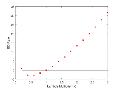
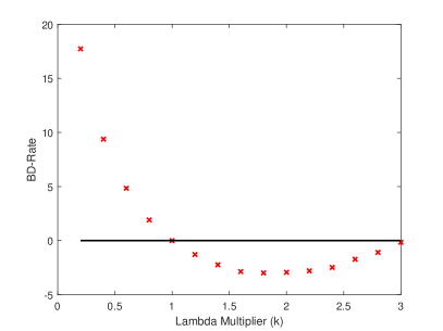
Figure 1: BD-Rate vs $k=[0.2:0.2:3]$ for two different clips (LiveMusic_1080P-6d1a and NewsClip_720P-7e56). The best performing BD-Rate gain is achieved at a different value for $k$ in each clip. Hence per-clip optimisation is sensible. The curve shape shows a global minimum implying that classic optimisation strategies would be successful.

In Figure 2, we report the BD-Rate improvement found in [13] to be achievable by such a direct optimisation of the Lagrangian Multiplier. In this graph, we see the BD-Rate improvement on the x-axis and the fraction of the dataset which was able to achieve that BD-Rate improvement or better. Ideally, we would want this curve to be as close to the top right as possible, as that would indicate all clips achieved high BD-Rate improvements. We will be using these results as our ground truth and upper bound for the deep learning systems described later in this paper. The key result of this work is that 95% of the clips had some BD-Rate improvement over the default Lagrangian Multiplier, with 46% of them showing a BD-Rate improvement of 1% or better.

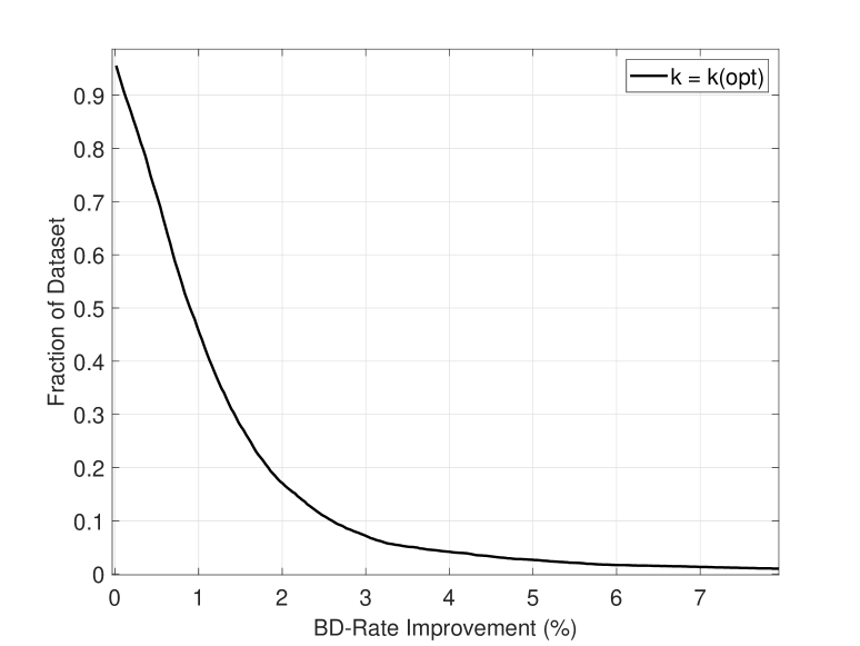
Figure 2: BD-Rate improvement vs fraction of dataset which achieves that improvement or better. We can see from this curve that the direct optimisation method was capable of achieving BD-Rate improvement in 95% of the clips in the corpus. We can also read off of this graph what fraction of the clips had a 1% or better BD-Rate improvement (47%) and what fraction of the clips had a 5% or better improvement (3%).

II-C Machine-Learning Prediction of $k$

The direct optimisation method [13] outlined in the previous section, provides positive results, however, it is computationally expensive. It takes on average 11.7 iterations, and, as each BD-rate computation takes 5 video encodes, finding the optimal $k$ takes $11.7\times 5\approx 60$ video encodes. This is manageable at small resolutions, but is computationally intensive at modern resolutions (720p and higher) and at scale.

Because of this, we have proposed in [14] to reduce the computational cost by using proxies (low resolutions, older codecs) to calculate $k$ in practice. We were able to get a reduction of $3.1\times$, while achieving 83% of the gain found by direct optimisation. To attempt at further reducing the computational cost, we also trained a machine learning system (Random Forest) based on encoding information given by the x265 encoder at CRF 33. The results, reported in the second row of Table II, show that the Random Forest model leads to an average BD-Rate improvement of 0.19% and is still some way away from the potential 1.87% improvement given by direct optimisation.

III Is the Current Lagrangian Multiplier Optimal Across a Modern Corpus?

Before exploring how to predict a better per-clip $k$, we propose first to investigate if $k=1$, as set in the MPEG standard, is indeed optimal for our corpus. What we propose here is to exhaustively calculate the BD-Rate over our corpus for values of $k$ in the range $k$=0:0.001:3. The average BD-Rate improvement for a given $k$ can be seen in Figure 3. The figure shows an improvement where $k$ is approximately 0.7:0.8, with a best average improvement coming at $k=0.782$. This also matches with the histogram of the optimal $k$ values found with direct optimisation on the corpus videos (see Figure 4). The following command invocation was used for all video encodes:

x265 --input SEQ.y4m --crf <XX> --tune-PSNR --psnr --output OUT.mp4

where SEQ and OUT are the filenames for the raw input file and output encoded video. Clips were encoded with <XX> in the range 22:5:42.

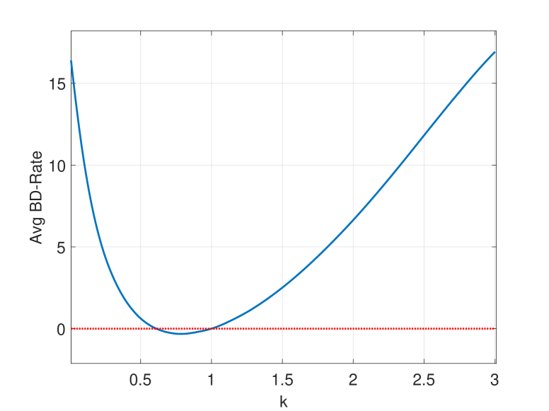
Figure 3: Average BD-Rate for a given k. Values of $k$ in the range $[0.7,0.8]$ give a clear average improvement (negative BD-rate) across the entire dataset.

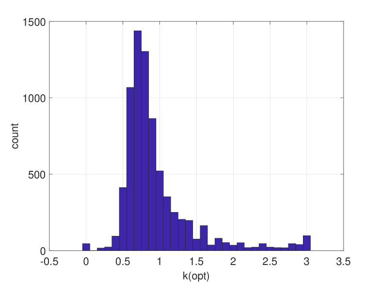
Figure 4: Histogram of optimum $k$ (and by extension optimum Lagrangian multiplier). The optimum is most frequently found in the $k$=0.7-0.8 range.

For $k=0.782$, about two-thirds of the clips have an improvement but it is worse for one-third of them (see Table II). Overall, we get an average gain of 0.32% across our corpus. This indicates that the Lagrangian Multiplier for HEVC may not be the best. This would imply that for HEVC, we should adjust the Lagrangian Multiplier to be $0.782\times$ its current value. However, this may be specific to our corpus and the operating points which we are using.

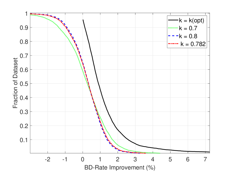
Figure 5: CDF plots of the BD-Rate improvement across our corpus when using $k$ = 0.7, 0.8 or 0.782. Ideally, we would want these plots to be as close as possible to the top right and coincide with the optimal per-clip plot (in black). We see for $k$ = 0.7, 0.8 or 0.782 positive BD-Rate improvements for 60-70% of the clips but worse performance for 30-40%.

IV Deep Learning for per clip Lagrangian Multiplier optimisation

We propose in this section to further explore the machine learning approach proposed in our previous work [14]. The main contributions are 1) to extend the feature set to per frame encoding statistics instead of global sequence statistics, 2) to include semantic visual features, and lastly 3) to employ a Deep Neural Network (DNN) instead of Random Forest.

IV-A Input Features

For this work, we collect two sets of features from each video from our corpus. As with our previous work [14], our first set of features comes from the statistics generated in the x265 encoder report.

TABLE I: List of Encoding Features used in Deep Learning system

Features Per Clip	Features Per Frame
Average Bitrate	Bits
Average PSNR (Y, U, V, Global)	I/P cost Ratio
Average I, P and B frame count	PSNR (Y,U,V)
Bitrate for I, P and B frames	Avg Chroma Distortion
I Frame PSNR (Y,U,V)	Average Residual Energy
P Frame PSNR (Y,U,V)	Avg Luma Level
B Frame PSNR (Y,U,V)	Avg Cb Level
	Avg Cr Level

We expand from [14] by also including the per frame features (see full list in Table I). This greatly expands the feature vector from 47 to 1523 features. The features are collected for a clip encoded with no modifications to the codec, at CRF 33.

In addition to these features, we also use the VGG16 network to generate semantic visual features about a single frame from each video sequence. We observed, indeed, that the nature of the clips content influenced the Lagrangian optimisation. The 1000 features from the 3c7 layer of VGG16 are used on a downsampled ($224\times 224$) median (75th) frame of the sequence. These two feature vectors are then concatenated into a combined feature vector of size 2523 for our model. Using the VGG features and NN architecture does come at a cost of increased complexity, but this may be preferable to multiple video encodes required for the direct optimisation method.

TABLE II: Summary of BD-R Gains results. This shows the $\%$ of clips which have any improvement, $\>0.1\%$ and $\>1\%$ improvement, as well as the best and average positive BD Rate improvement

Method	Clips with BD-R Gain of			Best	Avg Final
	$\geq 0\%$	$>0.1\%$	$>1\%$	Gain	Gain
Direct Optimisation	95%	89%	46%	23.9%	1.87%
Random Forest [14] (encoding features)	67%	28%	2%	8.5%	0.19%
Random Forest (encoding new)	68%	41%	11%	12%	0.23%
Random Forest (encoding + VGG features)	69%	65%	28%	18.3%	0.82%
$k=0.7$	58%	55%	25%	9.5%	0.55%
$k=0.8$	62%	56%	23%	16.9%	0.58%
$k=0.782$	62%	56%	23%	23.5%	0.63%
DNN (encoding + VGG features)	89%	84%	39%	14.9%	1.11%

IV-B Model & Training

TABLE III: Details of the Dense Layer sizes ($n$), dropout (0.1) and batch-normalisation (BN). All layers use the Gaussian Error Linear Unit (GELU) activation function.

layer id	1	2	3	4	5	6	7	8	9	10	11
$n$	1000	800	600	200	100	64	32	16	8	4	1
BN	✓	✓									✓
Dropout	✓	✓	✓					✓

Our model consists in a sequence of fully connected layers with GELU activation functions and Normalisation Layers. A full breakdown of the layers can be found in table III. The corpus is split 70%/30% between training and testing. The model was trained for 5000 epochs, using the SGD optimiser, a learning rate of 0.001 and a momentum of 0.9. The loss function is the mean absolute error between the predicted and directly optimised $k$.

V Results

Both our proposed deep learning model, and the Random Forest system outlined in [14] (with the updated feature set) yield BD-Rate improvements comparable to the direct optimisation. Figure 6 shows the portion of our test corpus which have a BD-Rate improvement. In these graphs, as well as the results presented in Table II, we see that roughly 95% of the clips had some BD-Rate improvement, with 46% of the corpus having a 1% or better BD-Rate improvement from direct optimisation. Our machine learning systems (Deep Learning and Random Forest from [14]) give positive results with 90% and 70% of the corpus getting a BD-Rate improvement but only 39% and 28% of the corpus getting a 1% or better BD-Rate improvement. We can see that while all three random forest implementations had a similar portion of the corpus show improvement, the amount of improvement was best using both the expanded encoding features along with the VGG features. The Random Forest and deep learning systems have a very similar performance on clips which yield 5% or better BD-Rate improvements. Both systems had roughly 1% of the corpus giving gains of 5% or more, but the Direct Optimiser was able to achieve 5% or better gains in approximately 5% of the clips. We believe that this is due to less training data available in the ”high improvement” range.

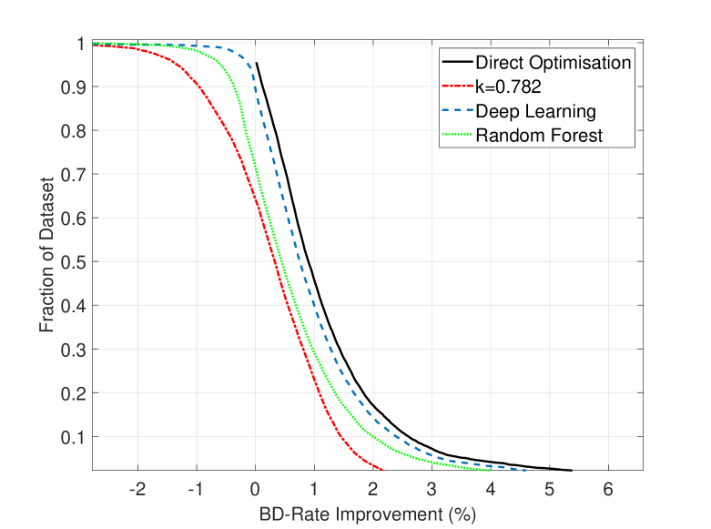
Figure 6: CDF plots of the BD-Rate improvement across our corpus for Random Forest [14] and our proposed DNN method. We see that both per-clip approaches outperform an overall adjustment of the Lagrangian multiplier ($k=0.782$) and that our network reaches near optimal performance.

We also see that both machine learning systems drastically outperform the best global Lagrangian multiplier adjustment ($k=0.782$), which confirms the benefits of using a per clip approach.

Table II also reports the average positive BD-Rate improvement as our Average Final BD-Rate Gain. This is the gain measured when our system is used as a post-process or optimised re-run of the encoder given an initial encode with default settings. The best BD-rate between the initial encode and the re-run defines the final BD-Rate Gain. This is the most likely use of systems of this kind, and can even be considered as a two-pass system. This allows us to take advantage of any improvements in BD-Rate from Lagrangian multiplier optimisation and default to the first default encode (unmodified Lagrangian Multiplier) in the case of worse performance. In this situation, we can see that our deep learning approach almost achieves what the direct optimiser does, at a fraction of the computational cost. The direct optimiser would have required on average sixty video encodes (12 RD-Curves) whereas our Deep Learning approach only required ten (2 RD-Curves) to get near comparable improvements.

VI Conclusion

In this paper, we have presented further data to support a per clip approach for the Lagrangian Multiplier within the HEVC codec. We build upon our direct optimisation results, by implementing a deep learning model capable of comparable results in a fraction ($1/6$) of the computational cost. 90% of our corpus shows some BD-Rate improvement with deep learning (compared to 95% of the corpus with direct optimisation). We also see that we can get approximately 1% BD-Rate savings across our entire corpus if we use the deep learning system as a supplement to the existing codec. In summary, our deep learning approach nears the direct optimiser results while using only $1/6^{th}$ of the computational cost. Future work will include investigating the deployment of this system for quality/distortion improvements at certain bitrates instead of BD-Rate gain as well as expansion to newer codecs like VVC.

References

- [1] S. Cass, “The age of the zettabyte cisco: the future of internet traffic is video [dataflow],” IEEE Spectrum, vol. 51, no. 3, pp. 68–68, 2014.
- [2] G. J. Sullivan, J.-R. Ohm, W.-J. Han, and T. Wiegand, “Overview of the high efficiency video coding (HEVC) standard,” IEEE Transactions on circuits and systems for video technology, vol. 22, no. 12, pp. 1649–1668, 2012.
- [3] T. Zhang and S. Mao, “An overview of emerging video coding standards,” GetMobile: Mobile Computing and Communications, vol. 22, no. 4, pp. 13–20, 2019.
- [4] B. Bross, J. Chen, S. Liu, and Y.-K. Wang, “Versatile video coding (draft 10),” ITU-T and ISO/IEC JVET-S2001, 2020.
- [5] D. Mukherjee, J. Bankoski, A. Grange, J. Han, J. Koleszar, P. Wilkins, Y. Xu, and R. Bultje, “The latest open-source video codec VP9-an overview and preliminary results,” in 2013 Picture Coding Symposium (PCS). IEEE, 2013, pp. 390–393.
- [6] Y. Chen, D. Murherjee, J. Han, A. Grange, Y. Xu, Z. Liu, S. Parker, C. Chen, H. Su, U. Joshi et al., “An overview of core coding tools in the av1 video codec,” in 2018 Picture Coding Symposium (PCS). IEEE, 2018, pp. 41–45.
- [7] G. J. Sullivan and T. Wiegand, “Rate-distortion optimization for video compression,” IEEE signal processing magazine, vol. 15, no. 6, pp. 74–90, 1998.
- [8] T. Wiegand and B. Girod, “Lagrange multiplier selection in hybrid video coder control,” in Proceedings 2001 International Conference on Image Processing, vol. 3. IEEE, 2001, pp. 542–545.
- [9] A. Ortega and K. Ramchandran, “Rate-distortion methods for image and video compression,” IEEE Signal processing magazine, vol. 15, no. 6, pp. 23–50, 1998.
- [10] G. J. Sullivan, J. Ohm, W. Han, and T. Wiegand, “Overview of the high efficiency video coding HEVC standard,” IEEE Transactions on Circuits and Systems for Video Technology, vol. 22, no. 12, pp. 1649–1668, Dec 2012.
- [11] I. Katsavounidis and L. Guo, “Video codec comparison using the dynamic optimizer framework,” in Applications of Digital Image Processing XLI, vol. 10752. International Society for Optics and Photonics, 2018, p. 107520Q.
- [12] M. Covell, M. Arjovsky, Y.-C. Lin, and A. Kokaram, “Optimizing transcoder quality targets using a neural network with an embedded bitrate model,” Electronic Imaging, vol. 2016, no. 2, pp. 1–7, 2016.
- [13] D. J. Ringis, F. Pitie, and A. Kokaram, “Per clip lagrangian multiplier optimisation for (HEVC),” Electronic Imaging, vol. 2020, no. 12, 2020. [Online]. Available: https://www.ingentaconnect.com/content/ist/ei/pre-prints/content-ei2020-ipas-136
- [14] D. J. Ringis, F. Pitié, and A. Kokaram, “Per-clip adaptive lagrangian multiplier optimisation with low-resolution proxies,” in Applications of Digital Image Processing XLIII, vol. 11510. International Society for Optics and Photonics, 2020, p. 115100E.
- [15] T. Wiegand, M. Lightstone, D. Mukherjee, T. G. Campbell, and S. K. Mitra, “Rate-distortion optimized mode selection for very low bit rate video coding and the emerging H. 263 standard,” IEEE Trans. on Circuits and Systems for Video Technology, vol. 6, no. 2, pp. 182–190, 1996.
- [16] C. Ma, K. Naser, V. Ricordel, P. Le Callet, and C. Qing, “An adaptive lagrange multiplier determination method for dynamic texture in HEVC,” in 2016 IEEE International Conference on Consumer Electronics-China (ICCE-China). IEEE, 2016, pp. 1–4.
- [17] A. M. Hamza, A. Abdelazim, and D. Ait-Boudaoud, “Parameter optimization in H. 265 rate-distortion by single frame semantic scene analysis,” Electronic Imaging, vol. 2019, no. 11, pp. 262–1, 2019.
- [18] F. Zhang and D. R. Bull, “Rate-distortion optimization using adaptive lagrange multipliers,” IEEE Transactions on Circuits and Systems for Video Technology, vol. 29, no. 10, pp. 3121–3131, Oct 2019.
- [19] M. A. Papadopoulos, F. Zhang, D. Agrafiotis, and D. Bull, “An adaptive QP offset determination method for HEVC,” in 2016 IEEE International Conference on Image Processing (ICIP), Sep. 2016, pp. 4220–4224.
- [20] A. Yang, H. Zeng, J. Chen, J. Zhu, and C. Cai, “Perceptual feature guided rate distortion optimization for high efficiency video coding,” Multidimensional Systems and Signal Processing, vol. 28, no. 4, pp. 1249–1266, 2017.
- [21] S. John, A. Gadde, and B. Adsumilli, “Rate distortion optimization over large scale video corpus with machine learning,” arXiv preprint arXiv:2008.12408, 2020.
- [22] Y. Wang, S. Inguva, and B. Adsumilli, “Youtube UGC dataset for video compression research,” in 2019 IEEE 21st International Workshop on Multimedia Signal Processing (MMSP), Sep. 2019, pp. 1–5.
- [23] Netflix, “Netflix Open Content,” https://opencontent.netflix.com/.
- [24] B. Ghanem and N. Ahuja, “Maximum margin distance learning for dynamic texture recognition,” in European Conference on Computer Vision. Springer, 2010, pp. 223–236.
- [25] J. Y. Lin, L. Jin, S. Hu, I. Katsavounidis, Z. Li, A. Aaron, and C.-C. J. Kuo, “Experimental design and analysis of jnd test on coded image/video,” in Applications of digital image processing XXXVIII, vol. 9599. International Society for Optics and Photonics, 2015, p. 95990Z.
- [26] Xiph.org, “Xiph.org Video Test Media,” https://media.xiph.org/video/derf/.