Sampling Strategies for Static Powergrid Models

Abstract

Machine learning and computational intelligence technologies gain more and more popularity as possible solution for issues related to the power grid. One of these issues, the power flow calculation, is an iterative method to compute the voltage magnitudes of the power grid’s buses from power values. Machine learning and, especially, artificial neural networks were successfully used as surrogates for the power flow calculation. Artificial neural networks highly rely on the quality and size of the training data, but this aspect of the process is apparently often neglected in the works we found. However, since the availability of high quality historical data for power grids is limited, we propose the Correlation Sampling algorithm. We show that this approach is able to cover a larger area of the sampling space compared to different random sampling algorithms from the literature and a copula-based approach, while at the same time inter-dependencies of the inputs are taken into account, which, from the other algorithms, only the copula-based approach does.

Keywords machine learning  $\cdot$ power grid  $\cdot$ powerflow  $\cdot$ surrogate models  $\cdot$ sampling  $\cdot$ correlation

1 Introduction

The knowledge about the current state of the power grid is, usually, limited to information about the power generation or consumption of the participants of the grid, either through prognosis or by estimations via default load profiles. However, a stable grid operation requires a certain frequency level (50 Hz in Europe) and certain voltage levels. Since only the power values are known, voltage information needs to be calculated, which is done with Power Flow (PF) analysis. The PF analysis is performed many times during the operation of power grids and the results can be used, e. g., for market analysis or short-term operational planning.

Since the PF analysis often requires to perform matrix inversion, a task with a high computational burden, there are many approaches to reduce this computation time. Active research for improvements of the more traditional methods can be found, e. g., in [1, 2, 3, 4]. On the other side, the advancement and application of Machine Learning (ML) models for energy systems has also increased in the past two decades. Mosavi et al. [5] reviewed a broad range of such applications, but PF analysis is barely mentioned, possibly due to their selection of relevant papers. [6] gave an overview about works regarding the closely related Optimal Power Flow (OPF) problem. OPF, however, is only a specific use case for PF. Nevertheless, ML for PF analysis is a field of active research and, especially, Artificial Neural Networks (ANNs) are often used with great performance, e. g., in [7], [8], and [9].

However, ANNs require a large amount of data, especially when the ANN becomes a Deep Neural Network (DNN). In our recent works in [10] and [11], we build different ML models, including a DNN, as a surrogate model for a Low Voltage (LV) power grid to avoid the costly PF analysis. One issue we identified concerns the availability and generation of training data. Our data set consisted of time series ranging over one year of data with a 15-minute resolution, resulting in about 35k data points for each time series or, translated to a ML task, about 35k training samples. Those samples need to be further split into training and test samples, which leaves even less data for the training. On the other side, creating new samples is not a trivial task (as we will show later in this paper), therefore, we decided to have a deeper look at the available data sets and sampling algorithms in the literature.

The rest of this paper is structured as follows. In section 2 we present the results of our investigation and discuss relevant literature. In section 3, we will have a short look at the basics of sampling strategies and discuss the challenges of power grid sampling in section 4. In section 5, we present our Correlation Sampling approach to overcome those issues. We compare and discuss our approach in section 6 and conclude our paper in section 7.

2 Related Work

The Open Power System Data (OPDS) platform [12] provides a hub for different data sets that can be used for electricity system modeling. In their work, the authors of the OPDS criticize that the quality and accessibility of publicly available data sets is often bad, require different files to download, have poor documentation, or are erroneous. Most of the data sets provided or linked on OPDS concern the power generation. The available load data sets are either highly aggregated hourly or monthly time series or small-scale household data sets (e. g., there is one with eleven households) that are hardly sufficient to model a distribution grid. Another good overview of data sets, especially for distribution grids, can be found in the wiki of the openmod initiative. The Simbench project [13] provides a large data set, ranging over all German voltage-levels, containing time series for loads and generation. Finally, there are the IEEE test cases, which mostly focus on North-American-style systems.

Besides using publicly available datasets, which may or may not be synthetic, there are also works that explicitly propose methodologies to create synthetic datasets. Hülk et al. [14] proposed a methodology that uses annual consumption data to generate a synthetic data set of the German energy system. This was extended by Amme et al. [15] with a focus on the Medium Voltage (MV) grid level. Likewise, in the research project SmartNord [16], a methodology was proposed to generate synthetic household loads that, once aggregated, follow the German default load profile H0. Most of these data sets, publicly available as well as synthetically generated, have in common that they range over one year with a time resolution of 15 minutes to one hour. This may be sufficient for power system modeling, but when it comes to the training of an DNN, either multiple data sets need to be combined for the training process or there is not much data left for validation of the model.

When neither of the above mentioned data sets fit or the data set is not large enough, sampling may be the solution. While this originates in the field of Probabilistic Load Flow (PLF), where inputs of the PF calculation are modeled as random variables [17], sampling is used in other PF-related fields as well. Cai et al. [18] use polynomial normal transformation together with Latin Hypercube Sampling (LHS) to build probability distribution models for PLF. Their models were able to handle correlated inputs and achieved better results on the IEEE 14-bus and 118-bus systems compared to a Simple Random Sampling (SRS) approach. Also in the field of PLF, Huang et al. [19] sampled with LHS as well but used D-vine copulas to model the inter-dependencies of wind speed between four wind farms. They evaluated the approach on a modified IEEE 33-bus system against SRS.

Lei et al. [20] used a Monte-Carlo simulation approach combined with an interior point algorithm to obtain feasible samples for OPF. They also did a sample pre-classification to group samples that share the same active constraints. The test cases were carried out on the IEEE 39, 57, and 118-bus systems as well as on a Polish 2383-bus system. Some works in the field of OPF simply use the base load values provided with most power grid models, e. g., the works in [21] and [22] use 10% and [23] even 70% deviation of the base load, although they, at least, did not sample from a uniform distribution.

In [24], the authors sampled a variation of the overall consumption and individual scaling factors for each load on the IEEE 14-bus system. Afterwards, loads are summed up and linearly scaled to match the overall consumption. Their use case was voltage control based on Deep Reinforcement Learning (DRL). Quite similar is the work of Diao et al. [25]. However, the authors used the the base load of the IEEE 14-bus system and created a load fluctuation between 80 % and 120 % of the base load values.

From this literature research we conclude that there are a couple of data sets available as well as several ways to generate synthetic data sets. Unfortunately, those data sets comprise not more than one year of data. Furthermore, we found different approaches to sample the power grid model, mostly one of the IEEE test cases, directly from different research fields. While in the PLF domain, the works consider actual time series of, e. g., wind farms for generation, this not always the case in the domains OPF and voltage control with DRL. In the works we discussed, the base load if often used for sampling. The resulting sampling data has a high chance to have completely different distributions than realistic (or synthetic) data, which can affect the quality of a prediction model. To this end, we propose a methodology that takes into account realistic time series and their inter-dependencies while at the same time preserve the flexibility of the sampling procedure.

3 Design of Experiments

The power grid model we used is a computer-based simulation model. As such, the Design of Experiments (DOE) literature would recommend space-filling designs [26, 27]. Space-filling designs aim to spread the sample points for each input evenly in the sample space. This can be achieved with Monte Carlo Sampling (MCS) (sometimes also called Simple Random Sampling (SRS)), i. e., using the uniform distribution independently for each input. Given that enough samples were drawn, this approach creates sampling designs that are nearly orthogonal, i. e., the inputs are uncorrelated. The LHS method is able to provide similar properties while at the same time requires usually less samples to to so.

In general, orthogonality and uniformly distributed inputs are desired properties of a sampling design since they can improve the validity of the prediction model created from that design. However, there are cases where some of the inputs in the original system-under-investigation are correlated and the power grid is a prime example for this. To be able to build a model that captures this behavior, the sample distributions for those inputs need to be correlated as well. One solution is to use Copulas, which were first proposed by [28]. Copulas have the capability to handle marginal distributions of random variables and dependencies separately. That is the reason increasing number of publications that have to deal with dependencies in power system modeling make use of Copulas, e. g., [19, 29].

4 Challenges of Power Grid Sampling

The power grid is a complex system, i. e., more basic DOE approaches for sampling and analysis cannot be applied to the power grid model without modifications. The complex inter-dependencies between the parts of the power grid make it hard to guarantee properties like orthogonality or uniformly distributed marginal distributions of the inputs without risking a decrease of the quality of the prediction model. To not consider certain correlations could even lead to ill-conditioned states of the power grid, where the PF calculation fails.

Gerster et al. [30] investigated sampling strategies for the determination of flexibility potentials at vertical system interconnections. One of their major conclusions concerns the application uniform sampling for each of the inputs. With increasing number of inputs, the samples suffer more and more from the convolution problem [30, 31, 32], i. e., at the vertical system interconnection point the actually covered space on the P-Q plane gets smaller the more inputs are involved.

Another challenge concerns the definition of the sample space of the inputs. While for most inputs, zero can be considered as minimum value, the maximum is not clearly defined. The base value attached to the publicly available power grid models and test cases may serve as reference value. But it is not a maximum value, since calculating the PF using base loads usually results in a healthy or, depending on the test case, slightly violated system state. It is also not an average value, which can be seen at the distributions of realistic load or generation profiles.

The advantage of using the base load as reference and creating sampling around those values with a certain deviation is that just the grid model itself without any time series data is required. This makes it convenient if only the general capabilities of an ML model should be explored. But unless the ML model is at least evaluated on realistic data, the model may only be a showcase for a certain ML algorithm on an environment that happens to be a power grid model. It does not necessarily imply that this model still performs well if realistic data is used.

To illustrate those issues and to motivate our own approach, we used the aforementioned Simbench project, which provides time series that are at least partially based on real datasets [13]. In one of our previous works, we already used the Simbench grid with code 1-LV-rural3--0-sw and, therefore, we used this grid here as well. Figure 1 illustrates the active power of a randomly selected household in the grid.

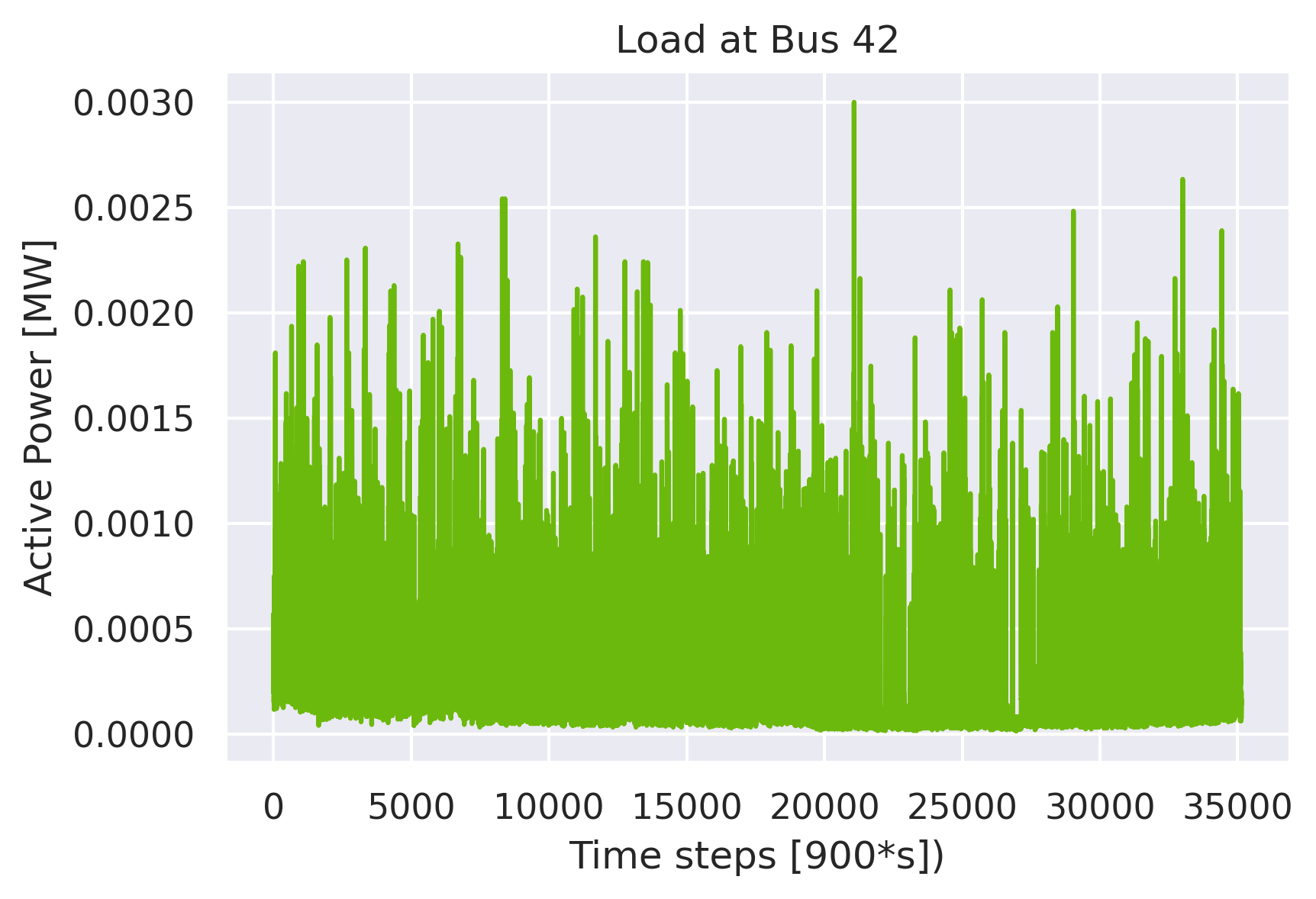
Figure 1: Active power time series of the load connected to bus 42 (randomly selected) over one year of simulated time. Taken from the Simbench grid 1-LV-rural3--0-sw.

The maximum peak power is 3 kW, which is the nominal power of the corresponding load in the grid model. In Figure 2 we plotted the histogram of this time series. Now it becomes obvious that most of the data is in the range between 0.0 and 0.5 kW. Actually, the mean value is $\approx$ 0.2657, the standard deviation $\approx$ 0.2781, and the median is at $\approx$ 0.1835. Sampling around the base load of 3 kW would result in samples, which, although valid, do not represent the original data and, consequently, which do not contain the necessary information for a ML model that should make predictions based on realistic input data.

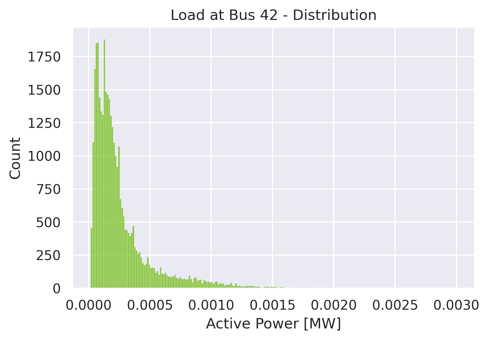
Figure 2: Histogram of the same active power time series as in Figure 1.

Next, we simulated the power grid using pandapower [33] for one year of simulated time. We follow [34] and plotted active against reactive power at the slack bus to get an estimate of the distribution of all of the simulation data and to be able to detect possible convolution problems. This can be seen in Figure 3.

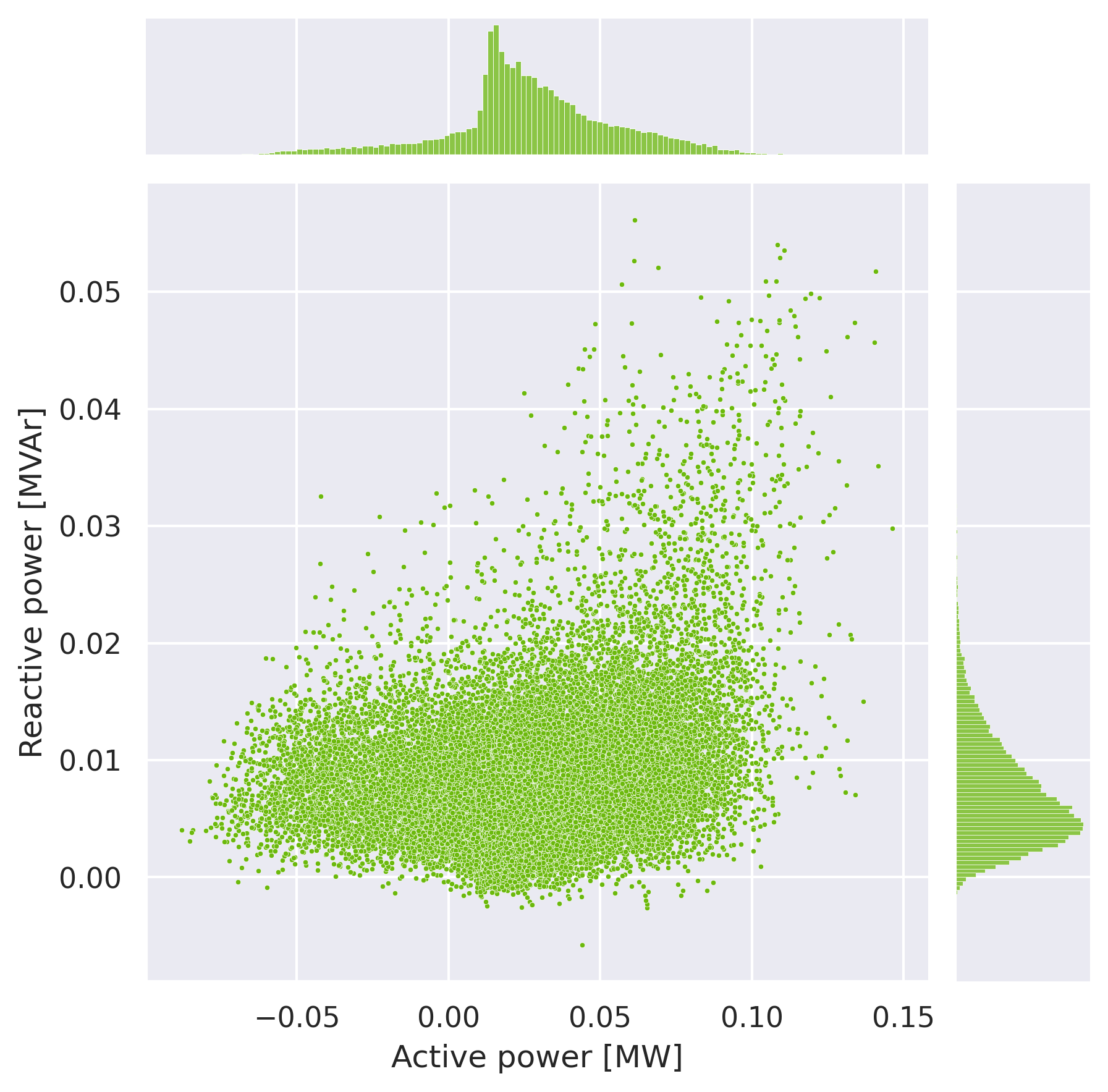
Figure 3: Plot of the active to reactive power plane at the slack bus using the data set that is included in the Simbench grid.

Now, we wanted to evaluate how well different sampling algorithms from the literature perform for this data set. We started with two variants of the SRS method; the first samples between 0 and the base load (Equation 1) and the second samples around the base load with a certain $\delta$ (Equation 2).

$$\mathbf{p}^{*}\thicksim\mathtt{Uniform}[0,\mathbf{p}_{b}]$$ (1)

$$\mathbf{p}^{*}\thicksim\mathtt{Uniform}[(1-\delta)\cdot\mathbf{p}_{b},(1+\delta)\cdot\mathbf{p}_{b}]$$ (2)

Here, $\mathbf{p}_{b}$ is the vector of base loads in the grid, $\delta$ is the deviation from the base load, and $\mathbf{p}^{*}$ is the vector of sampled power values. We used this formulas to generate 5000 samples for active and reactive power consumption as well as active power generation (the generators of the grid in-use had reactive power set to zero) with a $\delta$ of 0.5 in the second case. Afterwards, we calculated the PF for all samples to obtain the active and reactive power for the slack bus, just like above. The results can be seen in Figure 4. While all of the samples were feasible (i. e., the PF converged), we see that those distributions did not match at all.

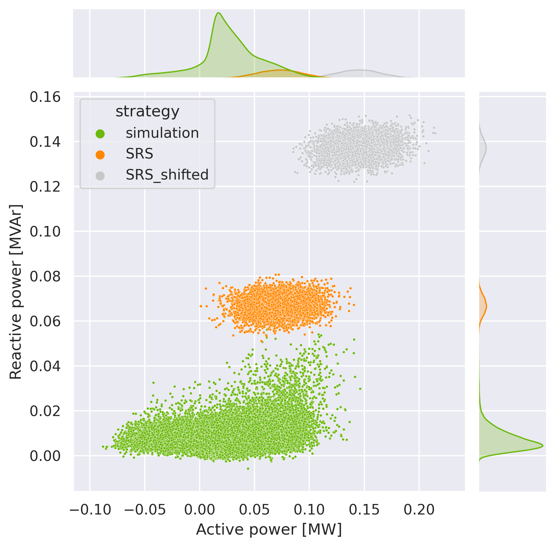
Figure 4: Plot of the active to reactive power plane at the slack bus. The lower dot cloud represents the results from original data sets. The middle dot cloud represents the results from the first SRS variant (sampling between zero and the base load) and the upper dot cloud the results from the second SRS variant (sampling around the base load).

A more advanced sampling strategy was used by Thayer et al. [24]. First, the authors used Equation 1 to sample active power on the interval [0.0, 1.0). Next, they varied the total active power loading $P^{\prime}$ uniformly between 60 % and 140% of the total active power loading $\overline{P}$ calculated from the base load. Each of the loads is scaled linearly with the factor $\overline{P^{\prime}}/\overline{P^{*}}$ where $\overline{P^{*}}$ is the total active power calculated from the samples $\mathbf{p}^{*}$. For reactive power $Q$, a power factor $pf$ for each load is drawn uniformly on the interval [0.8, 1.0) and $Q$ is calculated with

$$Q=P\cdot\mathtt{tan}(\mathtt{arccos}(pf))\cdot L,L\in\{-1,1\}.$$ (3)

The factor $L$ is a random variable with a chance of 10% to be -1 and, therefore, to flip the sign of $Q$. Like before, we created 5000 samples and calculated the PF results. The $P$ to $Q$ plot is shown in Figure 5. While a much larger part of the sampling space is covered, the areas of the original data and the sample data were completely different.

Figure 5: The results of advanced sampling algorithm were added to active-to-reactive power plot. The sign-flip of the algorithm in the partly mirrored dot cloud. Overall, the active power values were too high and, therefore, those samples did not cover the area of the original data.

Finally, we created a Gaussian copula to perform the same task. We used the python package copulas, which provides appropriate functions. The result is shown in Figure 6. The copula samples cover most of the space that is covered by the original data as well.

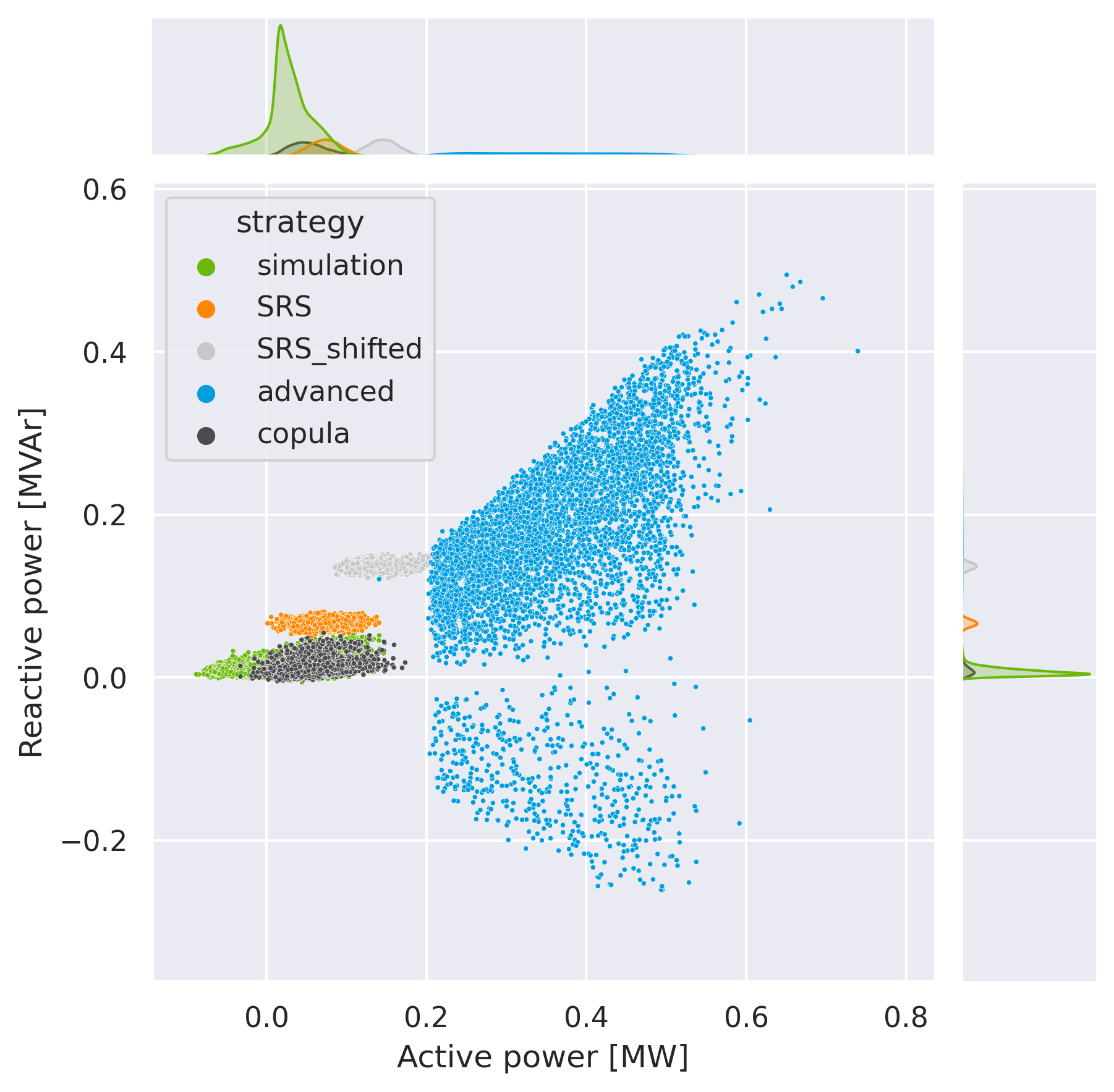
Figure 6: The results of the copula-based sampling were added to the plot. The darker dot cloud on top of the dot cloud of original data shows that copulas were able to reproduce the behavior of the original data.

We performed this experiment with different grid models and different time series and got similar results. Our conclusion is that SRS-based approaches are fine when no realistic data sets are available or the model prediction model will not not be used with realistic data sets. In any other case, copulas allow to create samples that represent the realistic data set.

However, there is one additional concern related to our specific use case. The copula samples might match the realistic data too well. One of the desired properties for sampling designs is that the sample points are evenly spread over the whole sample space. Although we don’t know the real boundaries of the sampling space, the SRS-based approaches cover valid areas of the sampling space that are not covered by the copula samples. We address this shortcoming with our sampling algorithm.

5 Correlation Sampling

The correlation sampling approach consists of two parts. In the first part, the correlations between the inputs are calculated, which is described in subsection 5.1. Those correlations are used in the second part to create a sampling design, described in subsection 5.2

5.1 Correlations

Naturally, the different entities that are connected to the power grid have inter-dependencies. Households follow similar patterns although there are different types of profiles. Photovoltaic modules are heavily dependent on the time of the day and weather conditions like cloudiness and solar radiation, which results in high correlations at spatially close positioned modules. Correlation can also be found between commercial facilities like different super markets or between several heating devices, which are dependent on temperature conditions.

Utilizing those inter-dependencies is also done in [19] to sample wind power plants for PLF and in [35] to assess the reliability of coalitions for the provision of ancillary services. Those inter-dependencies can also be found in the time series data sets for power grids, at least when the data set aims to be realistic. Therefore, we decided to use correlations, or, more specific partial correlations, to generate samples. The widely used correlation coefficient by Pearson [36] is defined as

$$\mathbf{r}_{XY}=\frac{\mathtt{cov}(X,Y)}{\sigma_{X}\sigma_{Y}}$$ (4)

with $X,Y$ being random variables, $\sigma_{X},\sigma_{Y}$ the standard deviation of $X$ and $Y$ and cov is the covariance. When more than two random variables are involved, other variables $\mathbf{Z}=(Z_{1},\dots,Z_{n})$ may have correlation to $X$ and $Y$ as well. Especially, $Z_{i}$ might be related to both $X$ and $Y$. To get the unbiased correlation between $X$ and $Y$, the partial correlation can be calculated.

$$\mathbf{r}_{XY|Z_{i}}=\frac{\mathbf{r}_{XY}-\mathbf{r}_{XZ_{i}}\cdot\mathbf{r}_{YZ_{i}}}{\sqrt{1-\mathbf{r}^{2}_{XZ_{i}}}\cdot\sqrt{1-\mathbf{r}^{2}_{YZ_{i}}}}$$ (5)

This can be described as two linear regression problems, the first between $Z_{i}$ and $X$ and the second between $Z_{i}$ and $Y$ [37]. Since the residuals of those linear regressions are uncorrelated to $Z_{i}$, the sample correlation can be calculated to obtain the partial correlation between $X$ and $Y$.

We will illustrate this using the data set from the 1-LV-rural3--0-sw Simbench grid, which was already used in the previous chapter. The Partial Correlation Matrix (PCM) $C$ between all of the inputs for the power grid over the full data set, displayed as heat map, can be seen in Figure 7.

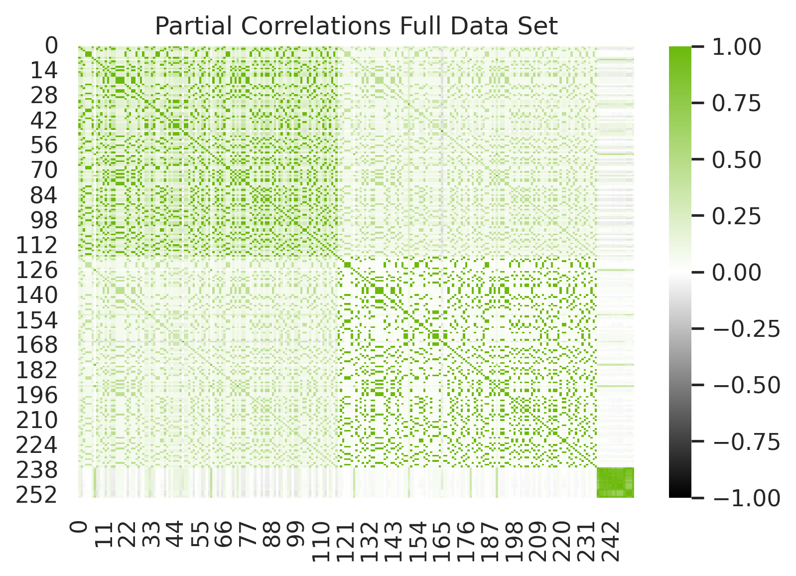
Figure 7: Heat map to illustrate the partial correlations between the inputs of data set provided by the Simbench power grid.

Although this PCM is sufficient for our sampling algorithm, we still used the whole data set to calculate the correlations. To overcome this, we selected a subset of the data set containing 2500 samples and calculated the PCM as $C^{\prime}$ again. This heat map can be seen in Figure 8.

Figure 8: Heat map to illustrate the partial correlations between the inputs. The correlations are calculated from a small subset of the data.

If you take a close look at both heat maps, you probably recognize similar "patterns". In fact, those PCMs are quite similar with a correlation factor of $\mathbf{r}_{CC^{\prime}}=0.98$, with duplicates (the lower left triangle of the matrix) included. The accumulated point-wise difference $C$ - $C^{\prime}$ sums up to -391.6 with a mean of -0.006, which indicates that the reduced PCM slightly over-estimates positive correlations. With a standard deviation of 0.055, we concluded that the reduced PCM is similar enough. Figure 9 shows the joint plot between the correlations from $C$ and $C^{\prime}$.

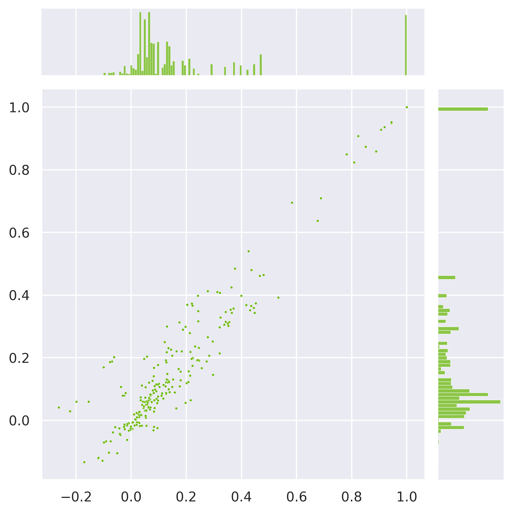
Figure 9: Joint plot over the correlation values from the full PCM and the reduced PCM.

5.2 Sampling

The next step concerned how to integrate the PCM $C^{\prime}$ into the sampling procedure. As it can be seen in Figure 9, most of the partial correlations are lower than 0.5 but there is another cluster between $\approx$ 0.85 and 1.0. To not suppress the randomness of the sampling, we defined a threshold $t$ of 0.85 and ignored all correlations that were lower. Each sample $\mathbf{s}$ is initially generated with the Dirichlet distribution, which was used by Gerster et al. [34] with good results. For each sample $\mathbf{s}_{i}$ in $\mathbf{s}$, all subsequent entries $\mathbf{s}_{j}$ with $i<j$, are adapted depending on their partial correlation $C^{\prime}_{ij}$:

$$\mathbf{s}_{j}=\begin{cases}\mathbf{s}_{j},~{}|C_{ij}|<t\\ \mathbf{s}_{i}+\mathbf{s}_{j}\cdot(1-C_{ij}),~{}C_{ij}>0\\ 1-\mathbf{s}_{i}+\mathbf{s}_{j}\cdot(1+C_{ij}),~{}C_{ij}<0\end{cases}$$ (6)

The general idea is to pull the value of sample $\mathbf{s}_{j}$ towards the value of sample $\mathbf{s}_{i}$ if they’re highly correlated. In Equation 6, cases two and three account for positive and negative correlation respectively.

We also applied some additional optimizations to better suit the current use case. First of all, we multiplied $\mathbf{s}_{j}$ with a normal distributed noise factor of 10% in cases where the correlation exceeds the threshold to relax the linear dependency towards $\mathbf{s}_{i}$. Second, to overcome some of the issues we’ve seen at the other sampling approaches, we calculated the sum of all values of this sample $\mathbf{s}$ and compared it to an interval [$s_{\mathtt{min}}$, $s_{\mathtt{max}}$]. When $\mathbf{s}$ is not in [$s_{\mathtt{min}}$, $s_{\mathtt{max}}$], $\mathbf{s}$ is discarded and sampled again.

The values $s_{\mathtt{min}}$ and $s_{\mathtt{max}}$ are derived from the data set again, by normalizing each time series individually, then building the sum for each time step, and, finally, assigning the minimum value to $s_{\mathtt{min}}$ and the maximum value to $s_{\mathtt{max}}$. However, since we used a reduced data set and, therefore, the interval [$s_{\mathtt{min}}$, $s_{\mathtt{max}}$] to small, we extended it by 20 % in each direction.

6 Evaluation

We used the described methodology to create samples like we did for the other sampling strategies. The $P$ to $Q$ plot at the slack bus is shown in Figure 10. It can be seen that the correlation samples not only cover the space of the real data but are also located in the regions largely around the real data. This even includes most of the space covered by the other sampling strategies.

Figure 10: The results of the correlation samples are added to the active-to-reactive power plot. A large area around the original data is covered, which includes even the areas of most of the other sampling algorithms.

We also re-calculated the partial correlations of the copula and correlation samples, the latter can be seen in Figure 11. The correlation between the copula-sampled PCM and the original full-data PCM is $\approx$ 0.98, which matches the correlation of the PCM of the reduced data set. For the correlation-sampled PCM, the is $\approx$ 0.864, which is less than the reduced data set but still very high. However, this difference may be one of the reasons why a larger area is covered.

Figure 11: Heat map of the PCMs of the sampling data created with correlation sampling. Visually, the partial correlation are closer to zero but still follow the same patterns.

We repeated this comparison with another power grid model, the CIGRE low voltage benchmark grid, in combination with synthetic time series data from Smart Nord, since we used this model in our previous works already. The results are shown in Figure 12 and this resembles all the issues and conclusions we identified for the Simbench grid, although the data sets are completely independent of each other.

Figure 12: The active-to-reactive power plot with different sampling algorithms for the CIGRE low voltage grid.

6.1 Discussion

The correlation sampling approach is, in its current state, a subject of experimentation. There are several parameters, like the correlation threshold or the number of samples that are used to calculate the partial correlations, which were determined experimentally and not for a special mathematical reason. There might be parameters that even lead to better results. Furthermore, only linear correlations are considered but in the data sets might be nonlinear correlations as well, which could be utilized to get more accurate samples.

On the other side, correlation sampling solved the issue we had with other sampling strategies, as can be seen in the evaluation. However, this is only a single but important step in the process of our use case: the training of a surrogate model to improve performance in simulation-based analysis. The evaluation of the correlation sampling approach in this use case is beyond the scope of this paper and will be subject of our next papers.

7 Conclusion and Future Work

In this paper, we presented a small literature research about available data sets for power system modeling, where to find them, and discussed some of the issues some of those data sets have. We also reviewed algorithms from the literature that were used to sample data sets for power grid simulation models and pointed out advantages and disadvantages. We presented our Correlation Sampling approach that aims to combine the advantages of the reviewed sampling algorithms. Correlation sampling achieved a larger coverage of the sampling space while at the same time taking inter-dependencies between the inputs into account.

Although those first results looks promising, we see a lot of potential for improvements of the algorithm. Additionally, the data set created with correlation sampling still needs to be used to build a surrogate model, which is the main purpose we developed that algorithm. We will present the results from those experiments in a future work.

References

- [1] LF Grisales-Noreña, OD Garzon-Rivera, CA Ramırez-Vanegas, OD Montoya, and CA Ramos-Paja. Application of the backward/forward sweep method for solving the power flow problem in dc networks with radial structure. In Journal of Physics: Conference Series, volume 1448, page 012012, 2020.
- [2] OD Montoya, AF Escobar, and VM Garrido. Power flow solution in direct current grids using the linear conjugate gradient approach. In Journal of Physics: Conference Series, volume 1448, page 012016, 2020.
- [3] Elefherios O Kontis, Georgios C Kryonidis, Angelos I Nousdilis, Kyriaki-Nefeli D Malamaki, and Grigoris K Papagiannis. Power flow analysis of islanded ac microgrids. In 2019 IEEE Milan PowerTech, pages 1–6. IEEE, 2019.
- [4] Zhichang Yuan, Yizhen Wang, Yue Yi, Chengshan Wang, Yuming Zhao, and Weijie Wen. Fast linear power flow algorithm for the study of steady-state performance of dc grid. IEEE Transactions on Power Systems, 34(6):4240–4248, 2019.
- [5] Amir Mosavi, Mohsen Salimi, Sina Faizollahzadeh Ardabili, Timon Rabczuk, Shahaboddin Shamshirband, and Annamaria R Varkonyi-Koczy. State of the art of machine learning models in energy systems, a systematic review. Energies, 12(7):1301, 2019.
- [6] Fouad Hasan, Amin Kargarian, and Ali Mohammadi. A survey on applications of machine learning for optimal power flow. In 2020 IEEE Texas Power and Energy Conference (TPEC), pages 1–6, Feb 2020.
- [7] Martin Nilsson, Lennart Soder, Jon Olauson, Robert Eriksson, Lars Nordström, and Göran N Ericsson. A machine learning method creating network models based on measurements. In 2018 Power Systems Computation Conference (PSCC), pages 1–7. IEEE, 2018.
- [8] Veerapandiyan Veerasamy, Noor Izzri Abdul Wahab, Rajeswari Ramachandran, Balasubramonian Madasamy, Muhammad Mansoor, Mohammad Lutfi Othman, and Hashim Hizam. A novel rk4-hopfield neural network for power flow analysis of power system. Applied Soft Computing, page 106346, 2020.
- [9] Balthazar Donon, Rémy Clément, Benjamin Donnot, Antoine Marot, Isabelle Guyon, and Marc Schoenauer. Neural networks for power flow: Graph neural solver. 2019.
- [10] Stephan Balduin, Martin Tröschel, and Sebastian Lehnhoff. Towards domain-specific surrogate models for smart grid co-simulation. Energy Informatics, 2(1):1–19, 2019.
- [11] Stephan Balduin, Tom Westermann, and Erika Puiutta. Evaluating different machine learning techniques as surrogate for low voltage grids. Energy Informatics, 3(1):1–12, 2020.
- [12] Frauke Wiese, Ingmar Schlecht, Wolf-Dieter Bunke, Clemens Gerbaulet, Lion Hirth, Martin Jahn, Friedrich Kunz, Casimir Lorenz, Jonathan Mühlenpfordt, Juliane Reimann, and Wolf-Peter Schill. Open power system data – frictionless data for electricity system modelling. Applied Energy, 236:401–409, 2019.
- [13] Christian Spalthoff, Dzanan Sarajlic, Chris Kittl, Simon Drauz, Tanja Kneiske, Christian Rehtanz, and Martin Braun. Simbench: Open source time series of power load, storage and generation for the simulation of electrical distribution grids. In International ETG-Congress 2019; ETG Symposium, pages 1–6. VDE, 2019.
- [14] Ludwig Hülk, Lukas Wienholt, Ilka Cußmann, Ulf Philipp Müller, Carsten Matke, and Editha Kötter. Allocation of annual electricity consumption and power generation capacities across multiple voltage levels in a high spatial resolution. International Journal of Sustainable Energy Planning and Management, 13:79–92, 2017.
- [15] J Amme, G Pleßmann, J Bühler, L Hülk, E Kötter, and P Schwaegerl. The ego grid model: An open-source and open-data based synthetic medium-voltage grid model for distribution power supply systems. In Journal of Physics: Conference Series, volume 977, page 012007. IOP Publishing, 2018.
- [16] Marita Blank, Timo Breithaupt, Jörg Bremer, Arne Dammasch, Steffen Garske, Thole Klingenberg, Stefanie Koch, Ontje Lünsdorf, Astrid Niesse, Stefan Scherfke, Lutz Hofmann, and Michael Sonnenschein. Smart nord final report. Technical report, Uni Hannover, 4 2015.
- [17] Peiyuan Chen, Zhe Chen, and Birgitte Bak-Jensen. Probabilistic load flow: A review. In 2008 Third International Conference on Electric Utility Deregulation and Restructuring and Power Technologies, pages 1586–1591. IEEE, 2008.
- [18] Defu Cai, Dongyuan Shi, and Jinfu Chen. Probabilistic load flow computation with polynomial normal transformation and latin hypercube sampling. IET Generation, Transmission & Distribution, 7(5):474–482, 2013.
- [19] Yueshan Huang, Shuheng Chen, Zhe Chen, Weihao Hu, and Qi Huang. Improved probabilistic load flow method based on d-vine copulas and latin hypercube sampling in distribution network with multiple wind generators. IET Generation, Transmission & Distribution, 14(5):893–899, 2020.
- [20] Xingyu Lei, Zhifang Yang, Juan Yu, Junbo Zhao, Qian Gao, and Hongxin Yu. Data-driven optimal power flow: A physics-informed machine learning approach. IEEE Transactions on Power Systems, 36(1):346–354, 2020.
- [21] Neel Guha, Zhecheng Wang, Matt Wytock, and Arun Majumdar. Machine learning for ac optimal power flow. arXiv preprint arXiv:1910.08842, 2019.
- [22] Xiang Pan, Tianyu Zhao, and Minghua Chen. Deepopf: Deep neural network for dc optimal power flow. In 2019 IEEE International Conference on Communications, Control, and Computing Technologies for Smart Grids (SmartGridComm), pages 1–6. IEEE, 2019.
- [23] Ahmed S Zamzam and Kyri Baker. Learning optimal solutions for extremely fast ac optimal power flow. In 2020 IEEE International Conference on Communications, Control, and Computing Technologies for Smart Grids (SmartGridComm), pages 1–6. IEEE, 2020.
- [24] Brandon L Thayer and Thomas J Overbye. Deep reinforcement learning for electric transmission voltage control. In 2020 IEEE Electric Power and Energy Conference (EPEC), pages 1–8. IEEE, 2020.
- [25] Ruisheng Diao, Zhiwei Wang, Di Shi, Qianyun Chang, Jiajun Duan, and Xiaohu Zhang. Autonomous voltage control for grid operation using deep reinforcement learning. In 2019 IEEE Power & Energy Society General Meeting (PESGM), pages 1–5. IEEE, 2019.
- [26] Angela Dean and Daniel Voss. Design and analysis of experiments. Springer, 1999.
- [27] Karl Siebertz, Thomas Hochkirchen, and D van Bebber. Statistische versuchsplanung. Springer, 2010.
- [28] A Sklar. Fonctions dé repartition à n dimension et leurs marges. Paris: Publications de l’Institut de statistique de l’Université de Paris, 8:229–231, 1959.
- [29] Defu Cai, Dongyuan Shi, and Jinfu Chen. Probabilistic load flow computation using copula and latin hypercube sampling. IET Generation, Transmission & Distribution, 8(9):1539–1549, 2014.
- [30] Johannes Gerster, Marcel Sarstedt, Eric M. S. P. Veith, Sebastian Lehnhoff, and Lutz Hofmann. Pointing out the convolution problem of stochastic aggregation methods for the determination of flexibility potentials at vertical system interconnections. In ENERGY 2021, The Eleventh International Conference on Smart Grids, Green Communications and IT Energy-aware Technologies, pages 37–37. IARIA, IARIA XPS Press, 2021.
- [31] Jörg Bremer and Sebastian Lehnhoff. Phase-space exploration of unit ensembles in energy management. at-Automatisierungstechnik, 68(2):89–96, 2020.
- [32] Joerg Bremer and Sebastian Lehnhoff. Unfolding ensemble training sets for improved support vector decoders in energy management. In ICAART (2), pages 322–329, 2018.
- [33] L. Thurner, A. Scheidler, F. Schäfer, J. Menke, J. Dollichon, F. Meier, S. Meinecke, and M. Braun. pandapower — an open-source python tool for convenient modeling, analysis, and optimization of electric power systems. IEEE Transactions on Power Systems, 33(6):6510–6521, Nov 2018.
- [34] Johannes Gerster, Sebastian Lehnhoff, Marcel Sarstedt, Lutz Hofmann, and Eric MSP Veith. Comparison of random sampling and heuristic optimization-based methods for determining the flexibility potential at vertical system interconnections. In 2021 IEEE PES Innovative Smart Grid Technologies Europe (ISGT Europe), pages 1–6. IEEE, 2021.
- [35] Marita Blank. Reliability Assessment of Coalitions for the Provision of Ancillary Services. PhD thesis, Universität Oldenburg, 2015.
- [36] Jacob Benesty, Jingdong Chen, Yiteng Huang, and Israel Cohen. Pearson correlation coefficient. In Noise reduction in speech processing, pages 37–40. Springer, 2009.
- [37] Joe Whittaker. Graphical models in applied multivariate statistics. Wiley Publishing, 2009.