Generalized Lindblad Master Equation for Measurement-Induced Phase Transition

Yi-Neng Zhou

Institute for Advanced Study, Tsinghua University, Beijing,100084, China

* zhou-yn19@mails.tsinghua.edu.cn

March 11, 2024

Abstract

The measurement-induced phase transition (MIPT) occurs when the system is evolving under unitary evolution together with local measurements followed by post-selection. We propose a generalized version of the Lindblad master equation as a continuous equation, to describe the dynamics of the second RΓ©nyi entropy in the MIPT. This generalized Lindblad equation explicitly takes into account the post-selection in the MIPT, which is realized as the Einstein-Podolsky-Rosen (EPR) state projection in the equation. Also, this generalized Lindblad equation preserves the Hermitian, unit trace, and positive definiteness of the density matrix. We further use the hard-core Bose-Hubbard model as a concrete example to numerically confirm that our generalized Lindblad equation is applicable to describing the MIPT.

Β 

Β 

1 Introduction

Recent years have seen major progress in the understanding of quantum entanglement, and the study of entanglement transitions that separate different entanglement phases have been wildly discussed. Since the unitary evolution of a closed system typically drives it towards volume-law scaling for the entanglement entropy of subsystems, adding local measurement in the evolution process has been raised as a method to restrict the growth of entanglement. The study of the entanglement transition gave rise to the concept of the measurement-induced phase transition (MIPT). In measurement-induced phase transition, the unitary evolution can establish the entanglement between different parts of the system, while the local projective measurements on the system are believed to destroy the entanglement between different parts of the system. Thus, there is a competing relation between the unitary evolution and local measurements, and therefore, the increase in measurement rate can lead to an entanglement phase transition [2, 3, 1, 6, 4, 5, 7]. This dynamical process in some cases can be mapped to a classical percolation problem, making it feasible for large-size classical simulation [8]. It also enables the study of the phase diagram and critical exponents in different regions [9, 11, 12, 10, 15, 13, 14]. The nature of this phase transition has been analyzed from different perspectives including classical statistical mechanics models [8, 16], information scrambling [17], quantum error corrections [18, 19] and symmetry breaking [20].

The methods of studying entropy dynamics under measurements include tensor network [21, 22, 23], matrix product state [24], random unitary circuit [25, 16]. However, it remains an open question to find an equation that is continuous in time to describe the entropy dynamics of a quantum system along this unitary evolution together with measurements. Also, the role of post-selection is essential in this entanglement phase transition since it excludes the entropy corresponding to the probability distribution of different measurement results, and thus makes it possible to obtain the entanglement transition. Therefore, it should be explicitly written in this continuity equation. Here, we consider the dynamics of the second RΓ©nyi entropy of the system under unitary evolution together with projective measurements, followed by post-selections to project a general mixed state to a pure state.

In this paper, we derive a dynamical equation of density matrix to describe the second RΓ©nyi entropy dynamics under unitary evolution and projective measurements that are followed by post-selections. This generalized Lindblad equation preserves the Hermitian, unit trace, and positive definiteness of the density matrix. Moreover, in this process, the entropy comes from two parts: the entanglement entropy of the system corresponding to different measurement results, and the entropy corresponding to the probability distribution of different measurement results. In the MIPT, we only care about the entropy of the former part, so we need to exclude the entropy of the latter part. In our equation, we use the measurement on a partial basis to directly exclude this part of entropy. Since the measurement on the partial basis is explicitly written in our equation, we can observe the entanglement phase transition by directly calculating the entanglement entropy from our equation. Thus, we do not need to run the same protocol many times and post-process the entropy results to observe this phase transition. Our generalized Lindblad equation thus provides a natural description of the entropy dynamics along this process.

2 The generalized Lindblad equation for measurement process

We first briefly review how to obtain a Lindblad-like equation that describes a system under unitary evolution together with frequent measurements [26, 27, 28, 29].
For a closed system under unitary evolution, the time evolution of the density matrix of the system follows:

βˆ‚Οβˆ‚t=βˆ’i​[H^,ρ].πœŒπ‘‘π‘–^𝐻𝜌\frac{\partial\rho}{\partial t}=-i[\hat{H},\rho]. (1)

Thus, to the first order of δ​t𝛿𝑑\delta t, we obtain

ρ​(t+δ​t)≃ρ​(t)βˆ’i​[H^,ρ​(t)]​δ​t+o​(δ​t)2.similar-to-or-equalsπœŒπ‘‘π›Ώπ‘‘πœŒπ‘‘π‘–^π»πœŒπ‘‘π›Ώπ‘‘π‘œsuperscript𝛿𝑑2\rho(t+\delta t)\simeq\rho(t)-i[\hat{H},\rho(t)]\delta t+o(\delta t)^{2}. (2)

Next, we consider the system being measured at an equal time interval δ​t𝛿𝑑\delta t. During two neighboring measurements, the system’s evolution is governed by H^^𝐻\hat{H}. Then, the density matrix after the measurements is

ρM​(t+δ​t)=βˆ‘aL^a​ρ​(t+δ​t)​L^a†.superscriptπœŒπ‘€π‘‘π›Ώπ‘‘subscriptπ‘Žsubscript^πΏπ‘ŽπœŒπ‘‘π›Ώπ‘‘superscriptsubscript^πΏπ‘Žβ€ \rho^{M}(t+\delta t)=\sum_{a}\hat{L}_{a}\rho(t+\delta t)\hat{L}_{a}^{\dagger}. (3)

Here, we use ρMsuperscriptπœŒπ‘€\rho^{M} to denote the density matrix after measurements (M)𝑀(M), and L^asubscript^πΏπ‘Ž\hat{L}_{a} is called the Lindblad operator or quantum jump operator. Here, a=1,…,nπ‘Ž1…𝑛a=1,...,n labels the possible quantum jumps resulting from measurements.

If we simply assume that the probability of the system being measured at time t+δ​t𝑑𝛿𝑑t+\delta t is P​(t+δ​t)𝑃𝑑𝛿𝑑P(t+\delta t), then the density matrix after this probabilistic measurement is:

ρM​(t+δ​t)=[1βˆ’P​(t+δ​t)]​ρ​(t+δ​t)+P​(t+δ​t)β€‹βˆ‘aL^a​ρ​(t+δ​t)​L^a†.superscriptπœŒπ‘€π‘‘π›Ώπ‘‘delimited-[]1π‘ƒπ‘‘π›Ώπ‘‘πœŒπ‘‘π›Ώπ‘‘π‘ƒπ‘‘π›Ώπ‘‘subscriptπ‘Žsubscript^πΏπ‘ŽπœŒπ‘‘π›Ώπ‘‘superscriptsubscript^πΏπ‘Žβ€ \rho^{M}(t+\delta t)=\left[1-P(t+\delta t)\right]\rho(t+\delta t)+P(t+\delta t)\sum_{a}\hat{L}_{a}\rho(t+\delta t)\hat{L}_{a}^{\dagger}. (4)

Here, we consider the system is projected to a complete basis

βˆ‘a=1nL^a†​L^a=ℐ,superscriptsubscriptπ‘Ž1𝑛superscriptsubscript^πΏπ‘Žβ€ subscript^πΏπ‘Žβ„\sum_{a=1}^{n}\hat{L}_{a}^{\dagger}\hat{L}_{a}=\mathcal{I}, (5)

and this assumption preserves the trace of density matrix along this measurement process. By assuming the completeness of measurement basis and taking the limit δ​tβ†’0→𝛿𝑑0\delta t\to 0 then we obtain a differential equation of density matrix

βˆ‚Οβˆ‚t=βˆ’i​[H,ρ​(t)]+η​(t)β€‹βˆ‘a=1n[L^a​ρ​(t)​L^aβ€ βˆ’12​{L^a†​L^a,ρ​(t)}].πœŒπ‘‘π‘–π»πœŒπ‘‘πœ‚π‘‘superscriptsubscriptπ‘Ž1𝑛delimited-[]subscript^πΏπ‘ŽπœŒπ‘‘superscriptsubscript^πΏπ‘Žβ€ 12superscriptsubscript^πΏπ‘Žβ€ subscript^πΏπ‘ŽπœŒπ‘‘\frac{\partial\rho}{\partial t}=-i\left[H,\rho(t)\right]+\eta(t)\sum_{a=1}^{n}\left[\hat{L}_{a}\rho(t)\hat{L}_{a}^{\dagger}-\frac{1}{2}\{\hat{L}_{a}^{\dagger}\hat{L}_{a},\rho(t)\}\right]. (6)

Here, η​(t)πœ‚π‘‘\eta(t) is the probability of the system being measured per unit of time, and it is defined as η​(t+δ​t)=P​(t+δ​t)δ​tπœ‚π‘‘π›Ώπ‘‘π‘ƒπ‘‘π›Ώπ‘‘π›Ώπ‘‘\eta(t+\delta t)=\frac{P(t+\delta t)}{\delta t}. Here, we suppose that there is no singularity in η​(t)πœ‚π‘‘\eta(t). This equation is the same as the Lindblad master equation if we regard the measurement rate η​(t)πœ‚π‘‘\eta(t) as the dissipation strength γ𝛾\gamma.
Also, we mention that here we assume the measurement is performed on a complete basis, thus the anti-commutator part of the Lindblad master equation is trivial and amounts to an identity matrix, therefore, the equation is a special case of the general Lindblad equation. Also, the system under unitary evolution together with the measurement process can be described in other ways. For instance, we can derive the Lindblad master equation from a weak measurement approach [30, 31, 12, 32], which is by coupling the system to an ancilla and then performing a projective measurement on it and use the operator-sum representation, then βˆ‘a=1nL^a†​L^a≠ℐsuperscriptsubscriptπ‘Ž1𝑛superscriptsubscript^πΏπ‘Žβ€ subscript^πΏπ‘Žβ„\sum_{a=1}^{n}\hat{L}_{a}^{\dagger}\hat{L}_{a}\neq\mathcal{I} in general. We put more discussion about the the assumption βˆ‘a=1nL^a†​L^a=ℐsuperscriptsubscriptπ‘Ž1𝑛superscriptsubscript^πΏπ‘Žβ€ subscript^πΏπ‘Žβ„\sum_{a=1}^{n}\hat{L}_{a}^{\dagger}\hat{L}_{a}=\mathcal{I} in the Eq.Β (6) and the β€œweak measurement” scenario where βˆ‘a=1nL^a†​L^a≠ℐsuperscriptsubscriptπ‘Ž1𝑛superscriptsubscript^πΏπ‘Žβ€ subscript^πΏπ‘Žβ„\sum_{a=1}^{n}\hat{L}_{a}^{\dagger}\hat{L}_{a}\neq\mathcal{I} in the section I of the supplementary[45].

3 The measurement process followed by post-selection

When one considers the case where the system is projected on a partial basis, the Eq.Β (6) is not able to describe the density matrix dynamics. Here, projection on a partial basis means we only save the result of the system being projected on some specific states b𝑏b where b=1,2,…,m𝑏12β€¦π‘šb=1,2,...,m and m<nπ‘šπ‘›m<n. To see the failure of the Eq.Β (6) in this case, we can first directly use the Eq.Β (6) by changing the summation on the right-hand side from a=1,…,nπ‘Ž1…𝑛a=1,...,n to a=1,…,mπ‘Ž1β€¦π‘ša=1,...,m. Then, we will find that this new equation does not preserve the trace of the density matrix. Therefore, to preserve the unit trace of the density matrix, we need to normalize the density matrix when the system has been measured. Thus, in comparison to the Eq.Β (4), after this probabilistic measurement and the followed post-selection, the density matrix becomes:

ρM​(t+δ​t)=[1βˆ’P​(t+δ​t)]​ρ​(t+δ​t)+P​(t+δ​t)β€‹βˆ‘a=1mL^a​ρ​(t+δ​t)​L^a†Tr​(βˆ‘b=1mL^b​ρ​(t)​L^b†).superscriptπœŒπ‘€π‘‘π›Ώπ‘‘delimited-[]1π‘ƒπ‘‘π›Ώπ‘‘πœŒπ‘‘π›Ώπ‘‘π‘ƒπ‘‘π›Ώπ‘‘superscriptsubscriptπ‘Ž1π‘šsubscript^πΏπ‘ŽπœŒπ‘‘π›Ώπ‘‘superscriptsubscript^πΏπ‘Žβ€ Trsuperscriptsubscript𝑏1π‘šsubscript^πΏπ‘πœŒπ‘‘superscriptsubscript^𝐿𝑏†\rho^{M}(t+\delta t)=\left[1-P(t+\delta t)\right]\rho(t+\delta t)+P(t+\delta t)\frac{\sum_{a=1}^{m}\hat{L}_{a}\rho(t+\delta t)\hat{L}_{a}^{\dagger}}{\mathrm{Tr}\left(\sum_{b=1}^{m}\hat{L}_{b}\rho(t)\hat{L}_{b}^{\dagger}\right)}. (7)

Here, the denominator on the right-hand side is the normalization factor due to post-selection. Similar to the Eq.Β (6), by taking the limit δ​tβ†’0→𝛿𝑑0\delta t\to 0, we further obtain:

βˆ‚Οβˆ‚t=βˆ’i​[H^,ρ​(t)]+η​(t)β€‹βˆ‘a=1mL^a​ρ​(t)​L^a†Tr​(βˆ‘b=1mL^b​ρ​(t)​L^b†)βˆ’Ξ·β€‹(t)2β€‹βˆ‘a=1n{L^a†​L^a,ρ​(t)}.πœŒπ‘‘π‘–^π»πœŒπ‘‘πœ‚π‘‘superscriptsubscriptπ‘Ž1π‘šsubscript^πΏπ‘ŽπœŒπ‘‘superscriptsubscript^πΏπ‘Žβ€ Trsuperscriptsubscript𝑏1π‘šsubscript^πΏπ‘πœŒπ‘‘superscriptsubscript^πΏπ‘β€ πœ‚π‘‘2superscriptsubscriptπ‘Ž1𝑛superscriptsubscript^πΏπ‘Žβ€ subscript^πΏπ‘ŽπœŒπ‘‘\frac{\partial\rho}{\partial t}=-i[\hat{H},\rho(t)]+\eta(t)\sum_{a=1}^{m}\frac{\hat{L}_{a}\rho(t)\hat{L}_{a}^{\dagger}}{\mathrm{Tr}\left(\sum_{b=1}^{m}\hat{L}_{b}\rho(t)\hat{L}_{b}^{\dagger}\right)}-\frac{\eta(t)}{2}\sum_{a=1}^{n}\{\hat{L}_{a}^{\dagger}\hat{L}_{a},\rho(t)\}. (8)

If we set m=nπ‘šπ‘›m=n which means we measure the system on a complete basis, we will find that the normalization factor Tr​(βˆ‘b=1nL^b​ρ​(t)​L^b†)=1Trsuperscriptsubscript𝑏1𝑛subscript^πΏπ‘πœŒπ‘‘superscriptsubscript^𝐿𝑏†1\mathrm{Tr}\left(\sum_{b=1}^{n}\hat{L}_{b}\rho(t)\hat{L}_{b}^{\dagger}\right)=1 since we assume the completeness condition of L^asubscript^πΏπ‘Ž\hat{L}_{a} in the Eq.Β (5). In this case, the Eq.Β (8) is the same as the case without post-selection in the Eq.Β (6).

For the general m<nπ‘šπ‘›m<n, the normalization factor βˆ‘b=1mTr​[L^b​ρ​(t+δ​t)​L^b†]superscriptsubscript𝑏1π‘šTrdelimited-[]subscript^πΏπ‘πœŒπ‘‘π›Ώπ‘‘superscriptsubscript^𝐿𝑏†\sum_{b=1}^{m}\mathrm{Tr}[\hat{L}_{b}\rho(t+\delta t)\hat{L}_{b}^{\dagger}] is generally not one and depends on ρ​(t)πœŒπ‘‘\rho(t), and this is a non-linear differential equation of ρ​(t)πœŒπ‘‘\rho(t) different from the Lindblad master equation. The non-trivial normalization factor given by the post-selection process leads to a different differential equation of the density matrix.

4 The general properties of the generalized Lindblad equation

A dynamical equation of the density matrix should preserve the Hermitian, unit trace, and positive definiteness properties of the density matrix. In the following, we will show that these three properties of the density matrix are preserved under the evolution of our generalized Lindblad equation.

We find that only the second term on the left-hand side of the Eq.Β (8) is different from the original Lindblad master equation, and we know the original Lindblad master equation preserves these three properties. Hence, we can simply compare the difference between the second term on the right-hand side of our generalized Lindblad equation and that of the original Lindblad equation.

Firstly, since βˆ‘a=1mL^a​ρ​(t)​L^a†Tr​(βˆ‘b=1mL^b​ρ​(t)​L^b†)superscriptsubscriptπ‘Ž1π‘šsubscript^πΏπ‘ŽπœŒπ‘‘superscriptsubscript^πΏπ‘Žβ€ Trsuperscriptsubscript𝑏1π‘šsubscript^πΏπ‘πœŒπ‘‘superscriptsubscript^𝐿𝑏†\sum_{a=1}^{m}\frac{\hat{L}_{a}\rho(t)\hat{L}_{a}^{\dagger}}{\mathrm{Tr}\left(\sum_{b=1}^{m}\hat{L}_{b}\rho(t)\hat{L}_{b}^{\dagger}\right)} is Hermitian, and Tr​[βˆ‘a=1mL^a​ρ​(t)​L^a†Tr​(βˆ‘b=1mL^b​ρ​(t)​L^b†)]=Tr​[12β€‹βˆ‘a=1n{L^a†​L^a,ρ​(t)}]Trdelimited-[]superscriptsubscriptπ‘Ž1π‘šsubscript^πΏπ‘ŽπœŒπ‘‘superscriptsubscript^πΏπ‘Žβ€ Trsuperscriptsubscript𝑏1π‘šsubscript^πΏπ‘πœŒπ‘‘superscriptsubscript^𝐿𝑏†Trdelimited-[]12superscriptsubscriptπ‘Ž1𝑛superscriptsubscript^πΏπ‘Žβ€ subscript^πΏπ‘ŽπœŒπ‘‘\mathrm{Tr}\left[\sum_{a=1}^{m}\frac{\hat{L}_{a}\rho(t)\hat{L}_{a}^{\dagger}}{\mathrm{Tr}\left(\sum_{b=1}^{m}\hat{L}_{b}\rho(t)\hat{L}_{b}^{\dagger}\right)}\right]=\mathrm{Tr}\left[\frac{1}{2}\sum_{a=1}^{n}\{\hat{L}_{a}^{\dagger}\hat{L}_{a},\rho(t)\}\right] =1absent1=1, it is easy to prove that ρ​(t)πœŒπ‘‘\rho(t) is Hermitian and preserves its unit trace along this evolution.

Secondly, the proof of positive definiteness is more involved, and it is as follows. We use the operator-sum representation of quantum channel [33]:

ρ​(t+d​t)=Ο΅d​t​[ρ​(t)]=βˆ‘a=0nMa^​ρ​(t)​M^a†.πœŒπ‘‘d𝑑subscriptitalic-Ο΅d𝑑delimited-[]πœŒπ‘‘superscriptsubscriptπ‘Ž0𝑛^subscriptπ‘€π‘ŽπœŒπ‘‘superscriptsubscript^π‘€π‘Žβ€ \rho(t+\mathop{}\!\mathrm{d}t)=\epsilon_{\mathop{}\!\mathrm{d}t}[\rho(t)]=\sum_{a=0}^{n}\hat{M_{a}}\rho(t)\hat{M}_{a}^{\dagger}. (9)

Here,

{M^0=I^+(βˆ’i​H^+K^)​d​tM^a=η​(t)​L^a​d​t,aβ‰ 0casessubscript^𝑀0absent^𝐼𝑖^𝐻^𝐾d𝑑subscript^π‘€π‘Žformulae-sequenceabsentπœ‚π‘‘subscript^πΏπ‘Ždπ‘‘π‘Ž0\begin{cases}\hat{M}_{0}&=\hat{I}+(-i\hat{H}+\hat{K})\mathop{}\!\mathrm{d}t\\ \hat{M}_{a}&=\sqrt{\eta(t)}\hat{L}_{a}\sqrt{\mathop{}\!\mathrm{d}t},\ \ \ \ a\neq 0\end{cases} (10)

with L^asubscript^πΏπ‘Ž\hat{L}_{a} representing quantum jump operators, and I^^𝐼\hat{I} representing the identity operator. Here, K^=βˆ’12​η​(t)β€‹βˆ‘a=1nL^a†​L^a^𝐾12πœ‚π‘‘superscriptsubscriptπ‘Ž1𝑛superscriptsubscript^πΏπ‘Žβ€ subscript^πΏπ‘Ž\hat{K}=-\frac{1}{2}\eta(t)\sum_{a=1}^{n}\hat{L}_{a}^{\dagger}\hat{L}_{a}. It is straightforward to see that this operator sum representation of quantum channel is equal to the Lindblad master equation the Eq.Β (6).

In our case, the density operator can be written in a similar operator-sum representation,

ρ​(t+d​t)=Ο΅d​tp​[ρ​(t)]=βˆ‘b=0mMb^​ρ​(t)​M^bβ€ πœŒπ‘‘d𝑑superscriptsubscriptitalic-Ο΅d𝑑𝑝delimited-[]πœŒπ‘‘superscriptsubscript𝑏0π‘š^subscriptπ‘€π‘πœŒπ‘‘superscriptsubscript^𝑀𝑏†\rho(t+\mathop{}\!\mathrm{d}t)=\epsilon_{\mathop{}\!\mathrm{d}t}^{p}[\rho(t)]=\sum_{b=0}^{m}\hat{M_{b}}\rho(t)\hat{M}_{b}^{\dagger} (11)

with

{M^0=I^+(βˆ’i​H^+K^)​d​tM^b=Ξ±t​η​(t)​L^b​d​t,b=1,…,m.casessubscript^𝑀0absent^𝐼𝑖^𝐻^𝐾d𝑑subscript^𝑀𝑏formulae-sequenceabsentsubscriptπ›Όπ‘‘πœ‚π‘‘subscript^𝐿𝑏d𝑑𝑏1β€¦π‘š\begin{cases}\hat{M}_{0}&=\hat{I}+(-i\hat{H}+\hat{K})\mathop{}\!\mathrm{d}t\\ \hat{M}_{b}&=\sqrt{\alpha_{t}\eta(t)}\hat{L}_{b}\sqrt{\mathop{}\!\mathrm{d}t},\ \ \ \ b=1,...,m.\end{cases} (12)

Here, K^=βˆ’12​η​(t)β€‹βˆ‘a=1nL^a†​L^a^𝐾12πœ‚π‘‘superscriptsubscriptπ‘Ž1𝑛superscriptsubscript^πΏπ‘Žβ€ subscript^πΏπ‘Ž\hat{K}=-\frac{1}{2}\eta(t)\sum_{a=1}^{n}\hat{L}_{a}^{\dagger}\hat{L}_{a}, and we also assume the completeness condition the Eq.Β (5). Here, the superscript p𝑝p in the Eq.Β (12) denotes the case with post-selection, and Ξ±t=[Tr​(βˆ‘b=1mL^b​ρ​(t)​L^b†)]βˆ’1subscript𝛼𝑑superscriptdelimited-[]Trsuperscriptsubscript𝑏1π‘šsubscript^πΏπ‘πœŒπ‘‘superscriptsubscript^𝐿𝑏†1\alpha_{t}=\left[\mathrm{Tr}\left(\sum_{b=1}^{m}\hat{L}_{b}\rho(t)\hat{L}_{b}^{\dagger}\right)\right]^{-1} is the normalization factor attributed to post-selection. Also, since m≀nπ‘šπ‘›m\leq n, the case where the system is being projected on the complete basis is included in the Eq.Β (11). We assume that at time t𝑑t, the density matrix is positive definite, i.e. ρ​(t)πœŒπ‘‘\rho(t) can be decomposed as ρ​(t)=βˆ‘jpj​|ψjβŸ©β€‹βŸ¨Οˆj|πœŒπ‘‘subscript𝑗subscript𝑝𝑗ketsubscriptπœ“π‘—brasubscriptπœ“π‘—\rho(t)=\sum_{j}p_{j}|\psi_{j}\rangle\langle\psi_{j}|, pjβ‰₯0subscript𝑝𝑗0p_{j}\geq 0. Thus, we find that

βŸ¨Ο•|ρ​(t+d​t)|Ο•βŸ©=βˆ‘b=0nβŸ¨Ο•|M^b​ρ​(t)​M^b†|Ο•βŸ©=βˆ‘b=0nβˆ‘jpj​|⟨ψj|M^b†|Ο•βŸ©|2β‰₯0,βˆ€Ο•.formulae-sequencequantum-operator-productitalic-Ο•πœŒπ‘‘d𝑑italic-Ο•superscriptsubscript𝑏0𝑛quantum-operator-productitalic-Ο•subscript^π‘€π‘πœŒπ‘‘superscriptsubscript^𝑀𝑏†italic-Ο•superscriptsubscript𝑏0𝑛subscript𝑗subscript𝑝𝑗superscriptquantum-operator-productsubscriptπœ“π‘—superscriptsubscript^𝑀𝑏†italic-Ο•20for-allitalic-Ο•\langle\phi|\rho(t+\mathop{}\!\mathrm{d}t)|\phi\rangle=\sum_{b=0}^{n}\langle\phi|\hat{M}_{b}\rho(t)\hat{M}_{b}^{\dagger}|\phi\rangle=\sum_{b=0}^{n}\sum_{j}p_{j}|\langle\psi_{j}|\hat{M}_{b}^{\dagger}|\phi\rangle|^{2}\geq 0,\ \ \forall\phi. (13)

Therefore, we conclude that ρ​(t+d​t)πœŒπ‘‘d𝑑\rho(t+\mathop{}\!\mathrm{d}t) is positive definite provided that ρ​(t)πœŒπ‘‘\rho(t) is positive definite. This completes the proof.

5 Entanglement entropy in the MIPT

We then consider entropy dynamics in the MIPT. We here simply focus on studying the second RΓ©nyi entropy defined as: S(2)=βˆ’log⁑[Tr​(ρ2)]superscript𝑆2Trsuperscript𝜌2S^{(2)}=-\log\left[\mathrm{Tr}(\rho^{2})\right]. We first notice that the Eq.Β (8) is not able to describe entropy dynamics along this process. The reason is as follows. Since the measurement will produce different results, the density matrix of the system during the evolution process is the summation of the density matrix corresponding to the different measurement results, and the weight of each result is its probability of it. We divide the system into subsystems A𝐴A and B𝐡B, and the reduced density matrix can be written as ρA=βˆ‘cpc​TrB​ρc=βˆ‘cpc​ρA,csubscript𝜌𝐴subscript𝑐subscript𝑝𝑐subscriptTr𝐡subscriptπœŒπ‘subscript𝑐subscript𝑝𝑐subscriptπœŒπ΄π‘\rho_{A}=\sum_{c}p_{c}\text{Tr}_{B}\rho_{c}=\sum_{c}p_{c}\rho_{A,c}. Here, pcsubscript𝑝𝑐p_{c} is the probability of getting ρcsubscriptπœŒπ‘\rho_{c}, and it satisfies βˆ‘cpc=1subscript𝑐subscript𝑝𝑐1\sum_{c}p_{c}=1. Therefore, it can be seen that the entanglement entropy comes from two parts: the entanglement entropy of the system corresponding to different measurement results βˆ’log⁑{Tr​[ρA,c2]}Trdelimited-[]superscriptsubscriptπœŒπ΄π‘2-\log\{\text{Tr}[\rho_{A,c}^{2}]\}, and the entropy corresponding to the probability distribution of different measurement results {pc}subscript𝑝𝑐\{p_{c}\}. In the MIPT, we are only concerned with the former part of entropy, and therefore we need to exclude the latter part. If the density matrix under the dynamic evolution described by the Eq.Β (8) is directly used in calculating entropy, we calculate the entanglement entropy of the mixed state obtained by the average of different measurement results:

SAtotalβ‰‘βˆ’log⁑{Tr​[(βˆ‘c=1mpc​ρA,c)2]}.subscriptsuperscript𝑆total𝐴Trdelimited-[]superscriptsuperscriptsubscript𝑐1π‘šsubscript𝑝𝑐subscriptπœŒπ΄π‘2S^{\text{total}}_{A}\equiv-\log\left\{\mathrm{Tr}\left[\left(\sum_{c=1}^{m}p_{c}\rho_{A,c}\right)^{2}\right]\right\}. (14)

Here, pcsubscript𝑝𝑐p_{c} is the probality of getting ρA,csubscriptπœŒπ΄π‘\rho_{A,c}, and it satisfies βˆ‘cpc=1subscript𝑐subscript𝑝𝑐1\sum_{c}p_{c}=1. Notice that not only the former part of entropy but also the latter part of entropy is included here. Therefore, the dynamics of entropy cannot be described only by the equation the Eq.Β (8).

To exclude the latter part of entropy in MIPT, we define a new type of entanglement entropy SAnewsuperscriptsubscript𝑆𝐴newS_{A}^{\text{new}} in this process as

SAnew=βˆ’log⁑{βˆ‘cpc~​[TrA​ρA,c2]}.superscriptsubscript𝑆𝐴newsubscript𝑐~subscript𝑝𝑐delimited-[]subscriptTr𝐴superscriptsubscriptπœŒπ΄π‘2S_{A}^{\text{new}}=-\log\left\{\sum_{c}\tilde{p_{c}}\left[\mathrm{Tr}_{A}\rho_{A,c}^{2}\right]\right\}. (15)

Here, pc~=pc2βˆ‘cβ€²pcβ€²2~subscript𝑝𝑐superscriptsubscript𝑝𝑐2subscriptsuperscript𝑐′superscriptsubscript𝑝superscript𝑐′2\tilde{p_{c}}=\frac{p_{c}^{2}}{\sum_{c^{\prime}}p_{c^{\prime}}^{2}}, and it also satisfies βˆ‘cpc~=1subscript𝑐~subscript𝑝𝑐1\sum_{c}\tilde{p_{c}}=1. To see that this definition of entanglement entropy the Eq.Β (15) does not take into account the entropy coming from the probability distribution {pc}subscript𝑝𝑐\{p_{c}\} in contrast to the Eq.Β (14), we consider a simple example. We assume that the system after evolution has probability p1=12subscript𝑝112p_{1}=\frac{1}{2} to be in ρA,1subscript𝜌𝐴1\rho_{A,1} with Tr​[ρA,12]=1Trdelimited-[]superscriptsubscript𝜌𝐴121\mathrm{Tr}[\rho_{A,1}^{2}]=1, and probability p2=12subscript𝑝212p_{2}=\frac{1}{2} to be in ρA,2subscript𝜌𝐴2\rho_{A,2} with Tr​[ρA,22]=1Trdelimited-[]superscriptsubscript𝜌𝐴221\mathrm{Tr}[\rho_{A,2}^{2}]=1. This means that in both cases, there is no entanglement entropy between subsystem A𝐴A and B𝐡B. Thus, the entropy only comes from the probability distribution {pc}={12,12}subscript𝑝𝑐1212\{p_{c}\}=\{\frac{1}{2},\frac{1}{2}\}. Also, we assume Tr​(ρA,1​ρA,2)<1Trsubscript𝜌𝐴1subscript𝜌𝐴21\mathrm{Tr}(\rho_{A,1}\rho_{A,2})<1 which means ρA,1subscript𝜌𝐴1\rho_{A,1} and ρA,1subscript𝜌𝐴1\rho_{A,1} are not the same, then we obtain SAnew=βˆ’log⁑[12+12]=0superscriptsubscript𝑆𝐴new12120S_{A}^{\text{new}}=-\log[\frac{1}{2}+\frac{1}{2}]=0 from the definition in the Eq.Β (15). However, if we use the SAtotalsubscriptsuperscript𝑆total𝐴S^{\text{total}}_{A} defined in the Eq.Β (14) to calculate the entanglement entropy, we obtain SAtotal=βˆ’log⁑[14+12​Tr​(ρA,1​ρA,2)+14]=βˆ’log⁑[12+12​Tr​(ρA,1​ρA,2)]>0superscriptsubscript𝑆𝐴total1412Trsubscript𝜌𝐴1subscript𝜌𝐴2141212Trsubscript𝜌𝐴1subscript𝜌𝐴20S_{A}^{\text{total}}=-\log[\frac{1}{4}+\frac{1}{2}\mathrm{Tr}(\rho_{A,1}\rho_{A,2})+\frac{1}{4}]=-\log[\frac{1}{2}+\frac{1}{2}\mathrm{Tr}(\rho_{A,1}\rho_{A,2})]>0. Therefore, this definition of entanglement entropy includes the entropy coming from the classical distribution {pc}subscript𝑝𝑐\{p_{c}\}. The proof of a more general case is written in the supplementary material [45].

Moreover, when all density matrix ρA,csubscriptπœŒπ΄π‘\rho_{A,c} are mutually orthogonal, it is straightforward to prove that SAtotalβ‰₯SAnewsuperscriptsubscript𝑆𝐴totalsuperscriptsubscript𝑆𝐴newS_{A}^{\text{total}}\geq S_{A}^{\text{new}} where the equality is taken when there is only one outcome with probability p1=1subscript𝑝11p_{1}=1. That means SAtotalβˆ’SAnewsuperscriptsubscript𝑆𝐴totalsuperscriptsubscript𝑆𝐴newS_{A}^{\text{total}}-S_{A}^{\text{new}} is non-negative as long as the entropy of probability distribution {pc}subscript𝑝𝑐\{p_{c}\} is non-zero. The details of this proof are written in the supplementary material [45].

6 The application of generalized Lindblad equation on the MIPT

In this section, we show that the entanglement entropy defined in the Eq.Β (15) can be obtained from a density matrix defined on a double space, and this double space density matrix’s evolution is governed by a generalized Lindblad equation that we will propose later.

The dynamics of the second RΓ©nyi entropy can be mapped to the dynamics of a wave function defined on a double space, and therefore the second RΓ©nyi entropy dynamics is more straightforward when it is written on a double space [34, 35]. We denote the two copies of the system on double space as the left(L) and the right(R) system, and we use ρDsuperscript𝜌𝐷\rho^{D} to denote the total density matrix of the double system. Given an initial density matrix ρ=βˆ‘m​nρm​n​|mβŸ©β€‹βŸ¨n|𝜌subscriptπ‘šπ‘›subscriptπœŒπ‘šπ‘›ketπ‘šbra𝑛\rho=\sum_{mn}\rho_{mn}|m\rangle\langle n|, the double state density matrix ρDsuperscript𝜌𝐷\rho^{D} is given by:

ρD=ΟβŠ—Ο=βˆ‘m​n​s​tρm​n,s​tD​|m⟩LβŠ—|s⟩Rβ€‹βŸ¨n|LβŠ—βŸ¨t|Rsuperscript𝜌𝐷tensor-product𝜌𝜌subscriptπ‘šπ‘›π‘ π‘‘tensor-producttensor-productsubscriptsuperscriptπœŒπ·π‘šπ‘›π‘ π‘‘subscriptketπ‘šπΏsubscriptket𝑠𝑅subscriptbra𝑛𝐿subscriptbra𝑑𝑅\rho^{D}=\rho\otimes\rho=\sum_{mnst}\rho^{D}_{mn,st}|m\rangle_{L}\otimes|s\rangle_{R}\langle n|_{L}\otimes\langle t|_{R} (16)

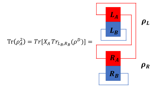
with ρm​n,s​tD=ρm​n​ρs​tsubscriptsuperscriptπœŒπ·π‘šπ‘›π‘ π‘‘subscriptπœŒπ‘šπ‘›subscriptπœŒπ‘ π‘‘\rho^{D}_{mn,st}=\rho_{mn}\rho_{st}. We can divide the system into subsystems A𝐴A and B𝐡B, and derive the entanglement entropy of subsystem A𝐴A from ρDsubscript𝜌𝐷\rho_{D}. Via a standard double space technique, the single system entropy SAβ‰‘βˆ’log⁑[Tr​(ρA2)]subscript𝑆𝐴Trsuperscriptsubscript𝜌𝐴2S_{A}\equiv-\log\left[\mathrm{Tr}(\rho_{A}^{2})\right] can be represented in the double space density matrix. Using TrA​(ρA2)=TrLA,RA​(XA​ρAβŠ—ΟA)=TrLA,RA​[XA​TrLB,RB​(ρD)]subscriptTr𝐴superscriptsubscript𝜌𝐴2subscriptTrsubscript𝐿𝐴subscript𝑅𝐴tensor-productsubscript𝑋𝐴subscript𝜌𝐴subscript𝜌𝐴subscriptTrsubscript𝐿𝐴subscript𝑅𝐴delimited-[]subscript𝑋𝐴subscriptTrsubscript𝐿𝐡subscript𝑅𝐡superscript𝜌𝐷\mathrm{Tr}_{A}(\rho_{A}^{2})=\mathrm{Tr}_{L_{A},R_{A}}(X_{A}\rho_{A}\otimes\rho_{A})=\mathrm{Tr}_{L_{A},R_{A}}\left[X_{A}\mathrm{Tr}_{L_{B},R_{B}}(\rho^{D})\right] , we have

SA=subscript𝑆𝐴absent\displaystyle S_{A}= βˆ’log⁑{TrLA,RA​[XA​TrLB,RB​(ρD)]},subscriptTrsubscript𝐿𝐴subscript𝑅𝐴delimited-[]subscript𝑋𝐴subscriptTrsubscript𝐿𝐡subscript𝑅𝐡superscript𝜌𝐷\displaystyle-\log\{\mathrm{Tr}_{L_{A},R_{A}}\left[X_{A}\mathrm{Tr}_{L_{B},R_{B}}(\rho^{D})\right]\}, (17)

and it is illustrated in the Fig.Β (1).

Refer to caption
Figure 1: The schematic diagram of calculating entanglement entropy from the double state density matrix ρDsuperscript𝜌𝐷\rho^{D}.

Here, ρAsubscript𝜌𝐴\rho_{A} is the reduced density matrix of subsystem A calculated from the total density matrix as ρA=TrB​[ρ]subscript𝜌𝐴subscriptTr𝐡delimited-[]𝜌\rho_{A}=\mathrm{Tr}_{B}[\rho]. Here, ρ𝜌\rho is the density matrix of the full system. X𝑋X is the swap operator defined as X​|α⟩L​|β⟩R=|β⟩L​|α⟩R𝑋subscriptket𝛼𝐿subscriptket𝛽𝑅subscriptket𝛽𝐿subscriptket𝛼𝑅X|\alpha\rangle_{L}|\beta\rangle_{R}=|\beta\rangle_{L}|\alpha\rangle_{R}. Here, XAsubscript𝑋𝐴X_{A} is the swap operator that acts on the subspace A𝐴A. LA​(LB)subscript𝐿𝐴subscript𝐿𝐡L_{A}(L_{B}) is the A𝐴A(B𝐡B) subsystem of the L𝐿L system, and RA​(RB)subscript𝑅𝐴subscript𝑅𝐡R_{A}(R_{B}) is the A𝐴A(B𝐡B) subsystem of the R𝑅R system.

When we consider the second Rényi entropy, to exclude the entropy coming from the classical distribution of different measurement results, we can enforce the condition that the L and the R system always collapse to the same state after measurement. In the double space, this condition means that the L and the R system are in the Einstein-Podolsky-Rosen (EPR) state. These above considerations motivate the equation of motion of the total density matrix ρDsuperscript𝜌𝐷\rho^{D}:

βˆ‚ΟDβˆ‚t=βˆ’i​[H^D,ρD​(t)]+η​(t)β€‹βˆ‘a=1nL^a,L​L^a,R​ρD​(t)​L^a,L†​L^a,R†Tr​(βˆ‘b=1nL^b,L​L^b,R​ρD​(t)​L^b,L†​L^b,R†)βˆ’Ξ·β€‹(t)2β€‹βˆ‘a.b=1n{L^a,L†​L^a,L​L^b,R†​L^b,R,ρD​(t)}.superscriptπœŒπ·π‘‘π‘–superscript^𝐻𝐷superscriptπœŒπ·π‘‘πœ‚π‘‘superscriptsubscriptπ‘Ž1𝑛subscript^πΏπ‘ŽπΏsubscript^πΏπ‘Žπ‘…superscriptπœŒπ·π‘‘superscriptsubscript^πΏπ‘ŽπΏβ€ superscriptsubscript^πΏπ‘Žπ‘…β€ Trsuperscriptsubscript𝑏1𝑛subscript^𝐿𝑏𝐿subscript^𝐿𝑏𝑅superscriptπœŒπ·π‘‘superscriptsubscript^𝐿𝑏𝐿†superscriptsubscript^πΏπ‘π‘…β€ πœ‚π‘‘2superscriptsubscriptformulae-sequenceπ‘Žπ‘1𝑛superscriptsubscript^πΏπ‘ŽπΏβ€ subscript^πΏπ‘ŽπΏsuperscriptsubscript^𝐿𝑏𝑅†subscript^𝐿𝑏𝑅superscriptπœŒπ·π‘‘\frac{\partial\rho^{D}}{\partial t}=-i[\hat{H}^{D},\rho^{D}(t)]+\eta(t)\sum_{a=1}^{n}\frac{\hat{L}_{a,L}\hat{L}_{a,R}\rho^{D}(t)\hat{L}_{a,L}^{\dagger}\hat{L}_{a,R}^{\dagger}}{\mathrm{Tr}\left(\sum_{b=1}^{n}\hat{L}_{b,L}\hat{L}_{b,R}\rho^{D}(t)\hat{L}_{b,L}^{\dagger}\hat{L}_{b,R}^{\dagger}\right)}-\frac{\eta(t)}{2}\sum_{a.b=1}^{n}\{\hat{L}_{a,L}^{\dagger}\hat{L}_{a,L}\hat{L}_{b,R}^{\dagger}\hat{L}_{b,R},\rho^{D}(t)\}. (18)

Here, L^a,Lsubscript^πΏπ‘ŽπΏ\hat{L}_{a,L} and L^a,Rsubscript^πΏπ‘Žπ‘…\hat{L}_{a,R} represent the jump operators acting on the L𝐿L and R𝑅R system respectively. Also, H^D=H^βŠ—I^+I^βŠ—H^superscript^𝐻𝐷tensor-product^𝐻^𝐼tensor-product^𝐼^𝐻\hat{H}^{D}=\hat{H}\otimes\hat{I}+\hat{I}\otimes\hat{H}, and I^^𝐼\hat{I} denotes the identity operator. This equation can be obtained by replacing ρ𝜌\rho by ρDsuperscript𝜌𝐷\rho^{D},H^^𝐻\hat{H} by H^Dsuperscript^𝐻𝐷\hat{H}^{D} and L^asubscript^πΏπ‘Ž\hat{L}_{a} by L^a,L​L^a,Rsubscript^πΏπ‘ŽπΏsubscript^πΏπ‘Žπ‘…\hat{L}_{a,L}\hat{L}_{a,R} in the Eq.Β (8). Similar to the discussion in the previous section, the numerator of the second term on the right-hand side βˆ‘a=1nL^a,L​L^a,R​ρD​(t)​L^a,L†​L^a,R†superscriptsubscriptπ‘Ž1𝑛subscript^πΏπ‘ŽπΏsubscript^πΏπ‘Žπ‘…superscriptπœŒπ·π‘‘superscriptsubscript^πΏπ‘ŽπΏβ€ superscriptsubscript^πΏπ‘Žπ‘…β€ \sum_{a=1}^{n}\hat{L}_{a,L}\hat{L}_{a,R}\rho^{D}(t)\hat{L}_{a,L}^{\dagger}\hat{L}_{a,R}^{\dagger} means that the double system is being projected on the EPR state since the quantum jump operator on the L𝐿L and R𝑅R system always being the same. It is a sharp contrast to the case where the numerator is chosen as βˆ‘a,b=1nL^a,L​L^b,R​ρD​(t)​L^a,L†​L^b,R†superscriptsubscriptπ‘Žπ‘1𝑛subscript^πΏπ‘ŽπΏsubscript^𝐿𝑏𝑅superscriptπœŒπ·π‘‘superscriptsubscript^πΏπ‘ŽπΏβ€ superscriptsubscript^𝐿𝑏𝑅†\sum_{a,b=1}^{n}\hat{L}_{a,L}\hat{L}_{b,R}\rho^{D}(t)\hat{L}_{a,L}^{\dagger}\hat{L}_{b,R}^{\dagger}. Since βˆ‘a,b=1nL^a,L​L^b,R​ρD​(t)​L^a,L†​L^b,R†superscriptsubscriptπ‘Žπ‘1𝑛subscript^πΏπ‘ŽπΏsubscript^𝐿𝑏𝑅superscriptπœŒπ·π‘‘superscriptsubscript^πΏπ‘ŽπΏβ€ superscriptsubscript^𝐿𝑏𝑅†\sum_{a,b=1}^{n}\hat{L}_{a,L}\hat{L}_{b,R}\rho^{D}(t)\hat{L}_{a,L}^{\dagger}\hat{L}_{b,R}^{\dagger} describes the system been projected on the complete basis of the double space, whereas EPR states are partial basis of the double space. The denominator on the right hand side Tr​(βˆ‘b=1nL^b,L​L^b,R​ρD​(t)​L^b,L†​L^b,R†)Trsuperscriptsubscript𝑏1𝑛subscript^𝐿𝑏𝐿subscript^𝐿𝑏𝑅superscriptπœŒπ·π‘‘superscriptsubscript^𝐿𝑏𝐿†superscriptsubscript^𝐿𝑏𝑅†\mathrm{Tr}\left(\sum_{b=1}^{n}\hat{L}_{b,L}\hat{L}_{b,R}\rho^{D}(t)\hat{L}_{b,L}^{\dagger}\hat{L}_{b,R}^{\dagger}\right) is the normalization factor resulting from post-selection. It is easy to see that this normalization factor is also non-trivial, making this equation a non-linear differential equation of ρDsuperscript𝜌𝐷\rho^{D}.

The generalized Lindblad equation Eq.Β (18) together with the entropy calculated through the double space technique the Eq.Β (17) are the central results of this paper. The essential property of the MIPT can be satisfied with this scheme, and the post-selection is explicitly embedded in the EPR state projection condition in the Eq.Β (18). These arguments rely on two steps:

  1. 1.

    Firstly, we will prove that the entropy formula the Eq.Β (17) for the evolved density matrix the Eq.Β (18) can be rewritten in the form of SAnewsuperscriptsubscript𝑆𝐴newS_{A}^{\text{new}} defined in the Eq.Β (15). This argument fundamentally requires the EPR state projection structure achieved by double space and the choice of Lindblad jump operators in the Eq.Β (18).

  2. 2.

    Secondly, as we find previously, SAnewsuperscriptsubscript𝑆𝐴newS_{A}^{\text{new}} in the Eq.Β (15) and the SAtotalsubscriptsuperscript𝑆total𝐴S^{\text{total}}_{A} in the Eq.Β (14) are conceptually different when describing the entanglement entropy. SAnewsuperscriptsubscript𝑆𝐴newS_{A}^{\text{new}} can exclude the entropy coming from the classical distribution {pc}subscript𝑝𝑐\{p_{c}\} by excluding the cross term pc​ρc​pc′​ρcβ€²subscript𝑝𝑐subscriptπœŒπ‘subscript𝑝superscript𝑐′subscript𝜌superscript𝑐′p_{c}\rho_{c}p_{c^{\prime}}\rho_{c^{\prime}} with cβ‰ c′𝑐superscript𝑐′c\neq c^{\prime} when calculating the entropy. In the aforementioned literature about MIPT [8, 10, 15], such exclusions are implemented by post-selection, while here it was naturally embedded in the framework of the generalized Lindblad equation.

We will then give a proof of the first argument. Similar to the previous section, the evolution of the double system density matrix can be represented in the operator-sum form

ρD​(t+d​t)=Ο΅d​t​[ρD​(t)]=βˆ‘b=0mM^bD​ρ0D​(t)​M^bD⁣†superscriptπœŒπ·π‘‘d𝑑subscriptitalic-Ο΅d𝑑delimited-[]superscriptπœŒπ·π‘‘superscriptsubscript𝑏0π‘šsuperscriptsubscript^𝑀𝑏𝐷superscriptsubscript𝜌0𝐷𝑑superscriptsubscript^𝑀𝑏𝐷†\rho^{D}(t+\mathop{}\!\mathrm{d}t)=\epsilon_{\mathop{}\!\mathrm{d}t}[\rho^{D}(t)]=\sum_{b=0}^{m}\hat{M}_{b}^{D}\rho_{0}^{D}(t)\hat{M}_{b}^{D\dagger} (19)

with

{M^0D=I^D+(βˆ’i​H^D+K^D)​d​tM^bD=Ξ±tD​η​(t)​L^b,L​L^b,R​d​t,b=1,…,m.casessuperscriptsubscript^𝑀0𝐷absentsuperscript^𝐼𝐷𝑖superscript^𝐻𝐷superscript^𝐾𝐷d𝑑superscriptsubscript^𝑀𝑏𝐷formulae-sequenceabsentsuperscriptsubscriptπ›Όπ‘‘π·πœ‚π‘‘subscript^𝐿𝑏𝐿subscript^𝐿𝑏𝑅d𝑑𝑏1β€¦π‘š\begin{cases}\hat{M}_{0}^{D}&=\hat{I}^{D}+(-i\hat{H}^{D}+\hat{K}^{D})\mathop{}\!\mathrm{d}t\\ \hat{M}_{b}^{D}&=\sqrt{\alpha_{t}^{D}\eta(t)}\hat{L}_{b,L}\hat{L}_{b,R}\sqrt{\mathop{}\!\mathrm{d}t},\ \ \ \ b=1,...,m.\end{cases} (20)

Here, K^D=K^L+K^R=βˆ’14​η​(t)β€‹βˆ‘a=1nL^a,L†​L^a,Lβˆ’14​η​(t)β€‹βˆ‘a=1nL^a,R†​L^a,Rsuperscript^𝐾𝐷subscript^𝐾𝐿subscript^𝐾𝑅14πœ‚π‘‘superscriptsubscriptπ‘Ž1𝑛superscriptsubscript^πΏπ‘ŽπΏβ€ subscript^πΏπ‘ŽπΏ14πœ‚π‘‘superscriptsubscriptπ‘Ž1𝑛superscriptsubscript^πΏπ‘Žπ‘…β€ subscript^πΏπ‘Žπ‘…\hat{K}^{D}=\hat{K}_{L}+\hat{K}_{R}=-\frac{1}{4}\eta(t)\sum_{a=1}^{n}\hat{L}_{a,L}^{\dagger}\hat{L}_{a,L}-\frac{1}{4}\eta(t)\sum_{a=1}^{n}\hat{L}_{a,R}^{\dagger}\hat{L}_{a,R}, and we also assume the completeness condition the Eq.Β (5). Then, by only keeping the first order of d​td𝑑\mathop{}\!\mathrm{d}t, we find that M^bDsuperscriptsubscript^𝑀𝑏𝐷\hat{M}_{b}^{D} can be rewritten as

{M^0D=M^0,LβŠ—M^0,RM^bD=M^b,LβŠ—M^b,R,b=1,…,mcasessuperscriptsubscript^𝑀0𝐷absenttensor-productsubscript^𝑀0𝐿subscript^𝑀0𝑅superscriptsubscript^𝑀𝑏𝐷formulae-sequenceabsenttensor-productsubscript^𝑀𝑏𝐿subscript^𝑀𝑏𝑅𝑏1β€¦π‘š\begin{cases}\hat{M}_{0}^{D}&=\hat{M}_{0,L}\otimes\hat{M}_{0,R}\\ \hat{M}_{b}^{D}&=\hat{M}_{b,L}\otimes\hat{M}_{b,R},\ \ \ b=1,...,m\end{cases} (21)

with

M^0=I^+(βˆ’i​H^+K^)​d​tM^b=[Ξ±tD​η​(t)]14​L^b​(d​t)14,subscript^𝑀0^𝐼𝑖^𝐻^𝐾d𝑑subscript^𝑀𝑏superscriptdelimited-[]superscriptsubscriptπ›Όπ‘‘π·πœ‚π‘‘14subscript^𝐿𝑏superscriptd𝑑14\begin{split}\hat{M}_{0}&=\hat{I}+(-i\hat{H}+\hat{K})\mathop{}\!\mathrm{d}t\\ \hat{M}_{b}&=\left[\alpha_{t}^{D}\eta(t)\right]^{\frac{1}{4}}\hat{L}_{b}(\mathop{}\!\mathrm{d}t)^{\frac{1}{4}},\\ \end{split}

and ​αtD=[Tr​(βˆ‘b=1nL^b,L​L^b,R​ρD​(t)​L^b,L†​L^b,R†)]βˆ’1andΒ superscriptsubscript𝛼𝑑𝐷superscriptdelimited-[]Trsuperscriptsubscript𝑏1𝑛subscript^𝐿𝑏𝐿subscript^𝐿𝑏𝑅superscriptπœŒπ·π‘‘superscriptsubscript^𝐿𝑏𝐿†superscriptsubscript^𝐿𝑏𝑅†1\text{and\ }\alpha_{t}^{D}=\left[\mathrm{Tr}\left(\sum_{b=1}^{n}\hat{L}_{b,L}\hat{L}_{b,R}\rho^{D}(t)\hat{L}_{b,L}^{\dagger}\hat{L}_{b,R}^{\dagger}\right)\right]^{-1} is the normalization factor attributed to post-selection in the double space. Then the entanglement entropy calculated from ρDsubscript𝜌𝐷\rho_{D} can be written as

SAD=superscriptsubscript𝑆𝐴𝐷absent\displaystyle S_{A}^{D}= βˆ’log⁑{TrLA,RA​[XA​TrLB,RB​(βˆ‘b=0mM^bD​ρ0D​M^bD⁣†)]}subscriptTrsubscript𝐿𝐴subscript𝑅𝐴delimited-[]subscript𝑋𝐴subscriptTrsubscript𝐿𝐡subscript𝑅𝐡superscriptsubscript𝑏0π‘šsuperscriptsubscript^𝑀𝑏𝐷superscriptsubscript𝜌0𝐷superscriptsubscript^𝑀𝑏𝐷†\displaystyle-\log\left\{\mathrm{Tr}_{L_{A},R_{A}}\left[X_{A}\mathrm{Tr}_{L_{B},R_{B}}(\sum_{b=0}^{m}\hat{M}_{b}^{D}\rho_{0}^{D}\hat{M}_{b}^{D\dagger})\right]\right\} (22)
=\displaystyle= βˆ’log{βˆ‘b=0mTrLA,RA[XATrLB,RB(M^b,Lρ0M^b,L†)βŠ—(M^b,Rρ0M^b,R†)]}\displaystyle-\log\{\sum_{b=0}^{m}\mathrm{Tr}_{L_{A},R_{A}}[X_{A}\mathrm{Tr}_{L_{B},R_{B}}(\hat{M}_{b,L}\rho_{0}\hat{M}_{b,L}^{\dagger})\otimes\quad(\hat{M}_{b,R}\rho_{0}\hat{M}_{b,R}^{\dagger})]\}
=\displaystyle= βˆ’log⁑{βˆ‘b=0mpb~​TrLA,RA​[XA​ρA,bβŠ—ΟA,b]}superscriptsubscript𝑏0π‘š~subscript𝑝𝑏subscriptTrsubscript𝐿𝐴subscript𝑅𝐴delimited-[]tensor-productsubscript𝑋𝐴subscriptπœŒπ΄π‘subscriptπœŒπ΄π‘\displaystyle-\log\left\{\sum_{b=0}^{m}\tilde{p_{b}}\mathrm{Tr}_{L_{A},R_{A}}\left[X_{A}\rho_{A,b}\otimes\rho_{A,b}\right]\right\}
=\displaystyle= βˆ’log⁑{βˆ‘b=0mpb~​TrA​[ρA,b2]}superscriptsubscript𝑏0π‘š~subscript𝑝𝑏subscriptTr𝐴delimited-[]superscriptsubscriptπœŒπ΄π‘2\displaystyle-\log\left\{\sum_{b=0}^{m}\tilde{p_{b}}\mathrm{Tr}_{A}\left[\rho_{A,b}^{2}\right]\right\}

with pb~=[Tr​(M^b​ρ0​(t)​M^b†)]2~subscript𝑝𝑏superscriptdelimited-[]Trsubscript^𝑀𝑏subscript𝜌0𝑑superscriptsubscript^𝑀𝑏†2\tilde{p_{b}}=\left[\mathrm{Tr}\left(\hat{M}_{b}\rho_{0}(t)\hat{M}_{b}^{\dagger}\right)\right]^{2} and ρA,b=TrB​[M^b​ρ0​(t)​M^b†]Tr​(M^b​ρ0​(t)​M^b†)subscriptπœŒπ΄π‘subscriptTr𝐡delimited-[]subscript^𝑀𝑏subscript𝜌0𝑑superscriptsubscript^𝑀𝑏†Trsubscript^𝑀𝑏subscript𝜌0𝑑superscriptsubscript^𝑀𝑏†\rho_{A,b}=\frac{\mathrm{Tr}_{B}\left[\hat{M}_{b}\rho_{0}(t)\hat{M}_{b}^{\dagger}\right]}{\mathrm{Tr}\left(\hat{M}_{b}\rho_{0}(t)\hat{M}_{b}^{\dagger}\right)}. Also, if we define Tr​(L^b​ρ0​(t)​L^b†)=pbTrsubscript^𝐿𝑏subscript𝜌0𝑑superscriptsubscript^𝐿𝑏†subscript𝑝𝑏\mathrm{Tr}\left(\hat{L}_{b}\rho_{0}(t)\hat{L}_{b}^{\dagger}\right)=p_{b}, then we have pb~=Ξ±tD​η​(t)​[Tr​(L^b​ρ0​(t)​L^b†)]2=η​(t)​pb2βˆ‘cpc2~subscript𝑝𝑏superscriptsubscriptπ›Όπ‘‘π·πœ‚π‘‘superscriptdelimited-[]Trsubscript^𝐿𝑏subscript𝜌0𝑑superscriptsubscript^𝐿𝑏†2πœ‚π‘‘superscriptsubscript𝑝𝑏2subscript𝑐superscriptsubscript𝑝𝑐2\tilde{p_{b}}=\alpha_{t}^{D}\eta(t)\left[\mathrm{Tr}\left(\hat{L}_{b}\rho_{0}(t)\hat{L}_{b}^{\dagger}\right)\right]^{2}=\eta(t)\frac{p_{b}^{2}}{\sum_{c}p_{c}^{2}} for b=1,…,n𝑏1…𝑛b=1,...,n. When we consider the case η​(t)=1πœ‚π‘‘1\eta(t)=1,which means that the probability of the system being measured per unit time is 1, this definition of pb~~subscript𝑝𝑏\tilde{p_{b}} is consistent with that of the new type of entanglement entropy SAnewsuperscriptsubscript𝑆𝐴newS_{A}^{\text{new}} in the Eq.Β (15). This completes the proof.

7 Numerical results

In this section, we numerically study the second RΓ©nyi entropy dynamics of a 1D hard-core Bose Hubbard [36] system under the Eq.Β (18) and (17) to show that this is consistent with the understanding that there could be an entanglement phase transition. The Hamiltonian of the hard-core Bose Hubbard system is

H^=βˆ’Jβ€‹βˆ‘βŸ¨i,j⟩b^i†​b^j+Uβ€‹βˆ‘βŸ¨i,j⟩n^i​n^j.^𝐻𝐽subscript𝑖𝑗superscriptsubscript^𝑏𝑖†subscript^π‘π‘—π‘ˆsubscript𝑖𝑗subscript^𝑛𝑖subscript^𝑛𝑗\hat{H}=-J\sum_{\langle i,j\rangle}\hat{b}_{i}^{\dagger}\hat{b}_{j}+U\sum_{\langle i,j\rangle}\hat{n}_{i}\hat{n}_{j}. (23)

Here, J𝐽J is the strength of the nearest neighbor hopping, and Uπ‘ˆU is the strength of the nearest neighbor interaction.

The system is driven by the generalized Lindblad equation the Eq.Β (18) in the double system, and we set η​(t)=Ξ³πœ‚π‘‘π›Ύ\eta(t)=\gamma as a time-independent measurement rate. Also, we set the projection measurements as

L^i,0=1L​(1βˆ’n^i),L^i,1=1L​n^i.formulae-sequencesubscript^𝐿𝑖01𝐿1subscript^𝑛𝑖subscript^𝐿𝑖11𝐿subscript^𝑛𝑖\hat{L}_{i,0}=\frac{1}{\sqrt{L}}(1-\hat{n}_{i}),\ \hat{L}_{i,1}=\frac{1}{\sqrt{L}}\hat{n}_{i}. (24)

Here i=1,2,…,Ns𝑖12…subscript𝑁𝑠i=1,2,...,N_{s}, and Nssubscript𝑁𝑠N_{s} is the total number of sites. Also, we further normalize the projection operators to satisfy the completeness condition of the measurement basis in Eq.Β (5). These projection operators mean that the environment is measuring the particle number on each site by projecting it on one of the particle number basis (|0⟩,|1⟩)ket0ket1(|0\rangle,|1\rangle). Here, |1⟩ket1|1\rangle denotes the site is occupied, and |0⟩ket0|0\rangle denotes the site is unoccupied.

In our following numerical calculation, we set J=U=1,Ns=6,Nb=3formulae-sequenceπ½π‘ˆ1formulae-sequencesubscript𝑁𝑠6subscript𝑁𝑏3J=U=1,N_{s}=6,N_{b}=3. Nbsubscript𝑁𝑏N_{b} is the total number of the hard-core boson. We denote the left half of the system as subsystem A𝐴A and the rest of it as subsystem B𝐡B. We then calculate the entanglement entropy SAsubscript𝑆𝐴S_{A} defined in the Eq.Β (17). We choose the initial state as a product state in the particle number basis |000111⟩ket000111|000111\rangle.

Refer to caption
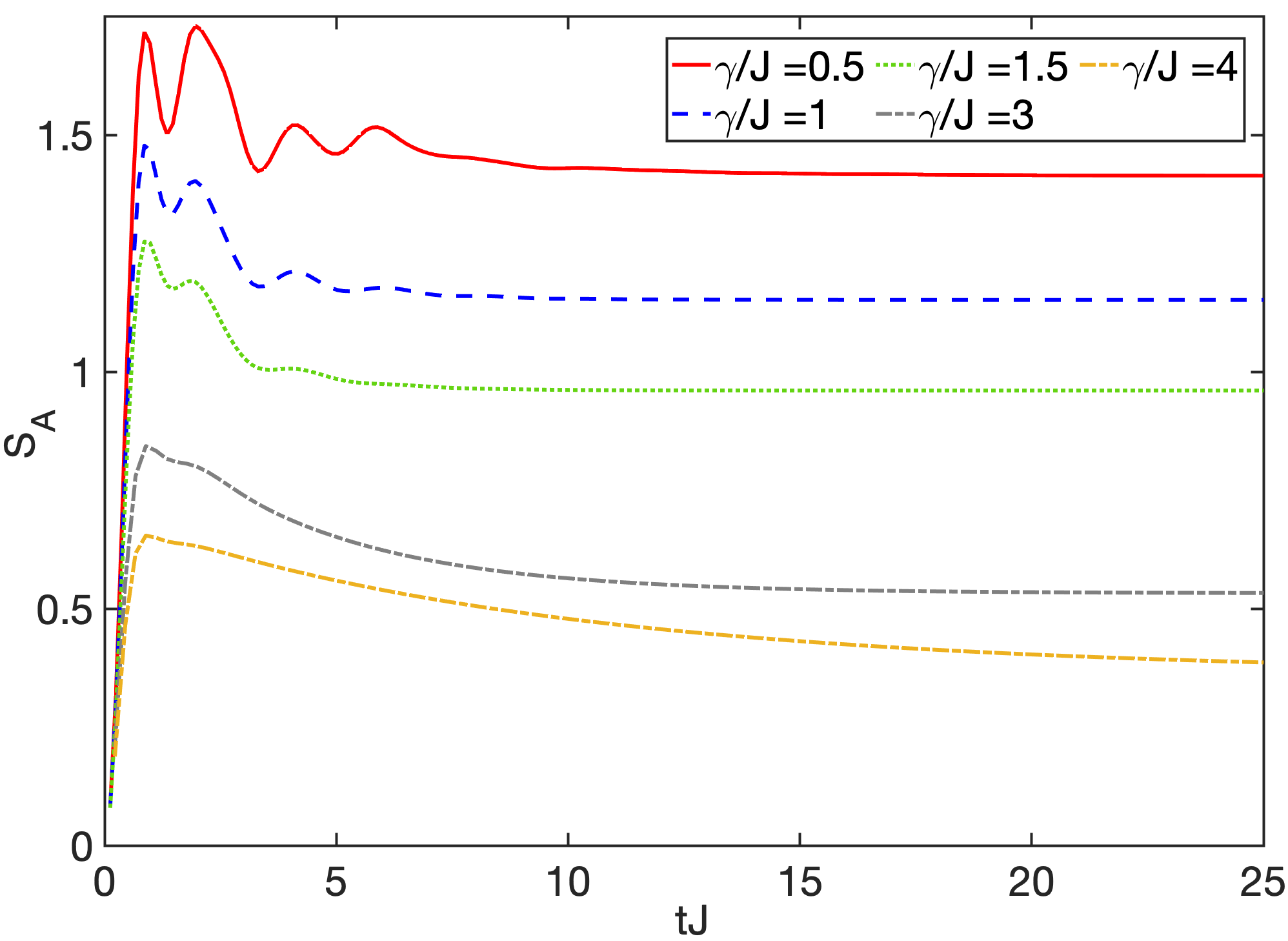
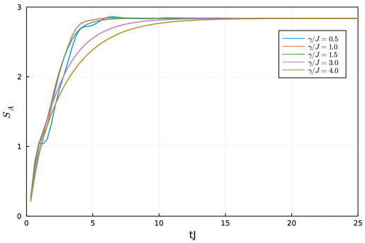
Figure 2: The dynamics of the entanglement entropy SAsubscript𝑆𝐴S_{A} as a function of t​J𝑑𝐽tJ. γ𝛾\gamma is the measurement rate. Different curves have different γ𝛾\gamma in the unit of J𝐽J. Here, U=Jπ‘ˆπ½U=J and the number of sites Ns=6subscript𝑁𝑠6N_{s}=6, and the number of bosons Nb=3subscript𝑁𝑏3N_{b}=3, and subsystem size LA=3subscript𝐿𝐴3L_{A}=3.
Refer to caption
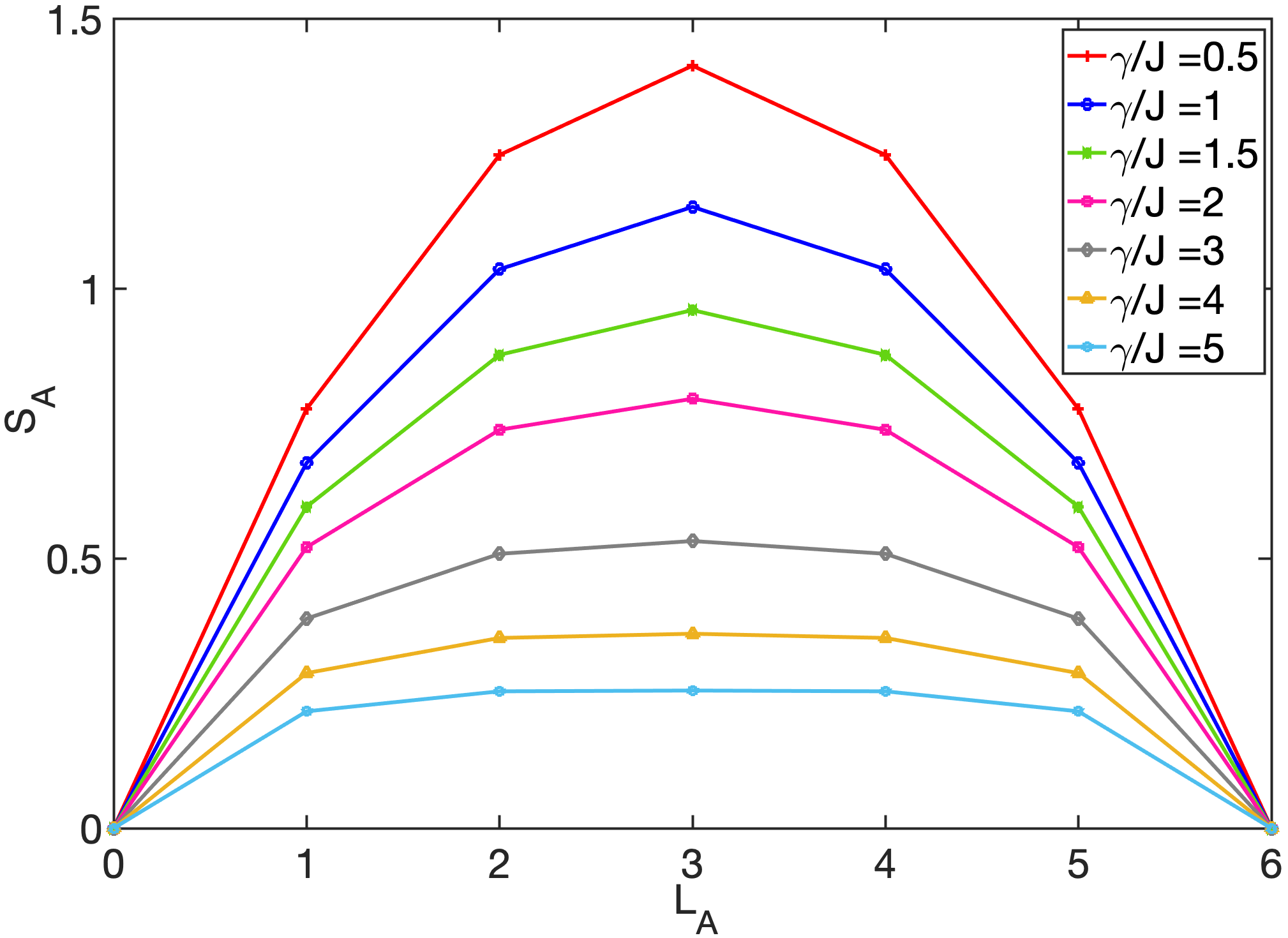
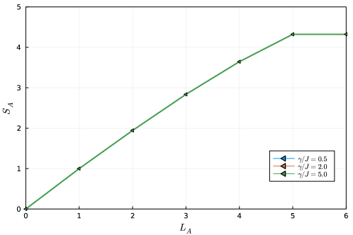
Figure 3: Saturation value of entanglement entropy SAsubscript𝑆𝐴S_{A} of the subsystem A𝐴A with different subsystem size LAsubscript𝐿𝐴L_{A}. Different curves have different γ𝛾\gamma in the unit of J𝐽J. Here, Ns=6subscript𝑁𝑠6N_{s}=6, Nb=3subscript𝑁𝑏3N_{b}=3, U/J=1π‘ˆπ½1U/J=1.

As shown in Fig.Β 2, the entanglement entropy SAsubscript𝑆𝐴S_{A} between subsystems A𝐴A and B𝐡B first quickly increases as expected in a normal chaotic system. However, it then decreases and saturates to a non-zero value. It indicates that measurements and the following post-selection process decrease the entanglement between subsystems. Also, we prove in the supplementary material [45] that the entanglement entropy is the same regardless of whether one computes partial trace over the subsystem A𝐴A or subsystem B𝐡B, and this explains why entanglement entropy SAsubscript𝑆𝐴S_{A} is symmetric to the half system size LAsubscript𝐿𝐴L_{A} axis (LA=Ns/2=3subscript𝐿𝐴subscript𝑁𝑠23L_{A}=N_{s}/2=3) in Fig.Β 2.

Moreover, from the result in Fig.Β 3, we find that when the measurement rate is small (Ξ³/J=0.5𝛾𝐽0.5\gamma/J=0.5) and LA<Ns/2subscript𝐿𝐴subscript𝑁𝑠2L_{A}<N_{s}/2, the entanglement entropy between the two subsystems A and B is almost linear in system size LAsubscript𝐿𝐴L_{A}. Whereas when the measurement rate is large (Ξ³/J=5𝛾𝐽5\gamma/J=5) and LA<Ns/2subscript𝐿𝐴subscript𝑁𝑠2L_{A}<N_{s}/2, the entanglement entropy is almost flat as LAsubscript𝐿𝐴L_{A} changes. In the MIPT, as the measurement rate γ𝛾\gamma increases, the entanglement entropy between the two subsystems A𝐴A and B𝐡B will change from volume-law to area-law, and our results are consistent with it. As expected, we observe here a reduction of the entanglement entropy as Ξ³/J𝛾𝐽\gamma/J is increased.

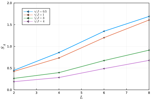
In the section E of the supplementary material [45], we use the quantum trajectory method to numerically calculate the entanglement entropy at different system size L𝐿L, and we find an almost linear growth in the entanglement entropy as the total system size increases at a small value of γ𝛾\gamma (Ξ³/J=0.5𝛾𝐽0.5\gamma/J=0.5), which indicates that there could be a volume-low scaling at a larger system size. In comparison, the entanglement entropy varies less as the size of the system increases at large values of γ𝛾\gamma (Ξ³/J=4𝛾𝐽4\gamma/J=4), which indicates that there could be a logarithmic critical scaling or an area law (constant) scaling at a larger system size. The details of the quantum trajectory methods that we have used here and more numerical results are also included in the supplementary material [45].

Thus, our results are in line with the understanding that there could be an entanglement phase transition in this process. Therefore, we use a concrete example to show that our generalized Lindblad equation the Eq.Β (18) can describe an entanglement phase transition as the measurement rate increases. Detailed information about the numerical integration technique used in producing Fig.Β 2 and Fig.Β 3 is added in the supplementary material [45].

Also, the numerical results of entanglement entropy calculated from the single-copy master equation the Eq.Β (8) are added in the supplementary material [45] for comparison. We find that there is no entanglement phase transition in this process, and there is no surprise since we mentioned in the section 5 that the entanglement entropy calculated from the single-copy master equation is SAtotalsubscriptsuperscript𝑆total𝐴S^{\text{total}}_{A} defined in the Eq.Β (14). Since SAtotalsubscriptsuperscript𝑆total𝐴S^{\text{total}}_{A} also includes the entropy corresponding to the probability distribution of different measurement results, there is no entanglement phase transition regarding this entanglement entropy.

8 Discussions

In this paper, we derive a generalized Lindblad equation for describing the dynamics of the system under the measurement process followed by post-selection. We emphasize that post-selection is essential in the non-linear differential the Eq.Β (18). Also, the generalized Lindblad equation the Eq.Β (18) preserves the Hermitian, unit trace, and positive definiteness of the density matrix. Furthermore, we generalize it to describe the second RΓ©nyi entropy dynamics in the MIPT, and we use a concrete model to demonstrate that our equation can indeed describe this entanglement transition as the measurement rate increases. Also, our generalized Lindblad equation can be simulated by the quantum trajectory methods [38, 42, 43, 44, 39, 41, 40] as the original Lindblad equation, and we consign the details to the Supplemental Material [45]. Therefore, the numerical simulation of these dissipative dynamics is feasible.

Moreover, the post-selection provides information about the probability distribution of measurement results. By using the information of the measurement results, we project the system to some pure states. Hence, we decrease the entropy of the system. Moreover, the Holevo information [37] defined as Ο‡:=Sv​(ρ)βˆ’βˆ‘ipi​Sv​(ρi)assignπœ’subscriptπ‘†π‘£πœŒsubscript𝑖subscript𝑝𝑖subscript𝑆𝑣subscriptπœŒπ‘–\chi:=S_{v}(\rho)-\sum_{i}p_{i}S_{v}(\rho_{i}) actually measures how much entropy on average is reduced once we learn the distribution {pi}subscript𝑝𝑖\{p_{i}\}. Here, Svsubscript𝑆𝑣S_{v} is the von Neumann entropy. Thus, if we measure von Neumann entropy in the MIPT, we find that the amount of entropy decreased by measurement and post-selection is just the Holevo information. The decrease of entropy by the measurement and post-selection process is owing to gaining accessible information about the measurement results.

The results we have presented here suggest some further directions that are worth exploring. It will be enlightening to analytically calculate the entropy from our generalized Lindblad equation. Also, It will be interesting to explore the Holevo information in the MIPT and try to understand this phase transition from the perspective of getting accessible classical information. It is also interesting to experimentally realize this generalized Lindblad equation by coupling the system to a bath and designing the form of interaction to satisfy the normalization factor of our generalized Lindblad equation. Therefore, we may further find some direct experimental access to the entanglement phase transition.

Acknowledgments

We thank Hui Zhai, Pengfei Zhang, and Tian-Gang Zhou for helpful discussion and for carefully reading the manuscript.

References

  • [1] B. Skinner, J. Ruhman, and A. Nahum, Measurement-Induced Phase Transitions in the Dynamics of Entanglement, Phys. Rev. X 9, 031009 (2019).
  • [2] Y. Li, X. Chen, and M. P. A. Fisher, Quantum Zeno Effect and the Many-Body Entanglement Transition, Phys. Rev. B 98, 205136 (2018).
  • [3] Y. Li, X. Chen, and M. P. A. Fisher, Measurement-Driven Entanglement Transition in Hybrid Quantum Circuits, Phys. Rev. B 100, 134306 (2019).
  • [4] A. Chan, R. M. Nandkishore, M. Pretko, and G. Smith, Unitary-Projective Entanglement Dynamics, Phys. Rev. B 99, 224307 (2019).
  • [5] G. Mazzucchi, W. Kozlowski, S. F. Caballero-Benitez, T. J. Elliott, and I. B. Mekhov, Quantum Measurement-Induced Dynamics of Many-Body Ultracold Bosonic and Fermionic Systems in Optical Lattices, Phys. Rev. A 93, 023632 (2016).
  • [6] M. Szyniszewski, A. Romito, and H. Schomerus, Entanglement Transition from Variable-Strength Weak Measurements, Phys. Rev. B 100, 064204 (2019).
  • [7] M. J. Gullans and D. A. Huse, Scalable Probes of Measurement-Induced Criticality, Phys. Rev. Lett. 125, 070606 (2020).
  • [8] C.-M. Jian, Y.-Z. You, R. Vasseur, and A. W. W. Ludwig, Measurement-Induced Criticality in Random Quantum Circuits, Phys. Rev. B 101, 104302 (2020).
  • [9] A. Lavasani, Y. Alavirad, and M. Barkeshli, Measurement-Induced Topological Entanglement Transitions in Symmetric Random Quantum Circuits, Nat. Phys. 17, 3 (2021).
  • [10] Y. Fuji and Y. Ashida, Measurement-Induced Quantum Criticality under Continuous Monitoring, Phys. Rev. B 102, 054302 (2020).
  • [11] O. Alberton, M. Buchhold, and S. Diehl, Entanglement Transition in a Monitored Free-Fermion Chain: From Extended Criticality to Area Law, Phys. Rev. Lett. 126, 170602 (2021).
  • [12] X. Turkeshi, A. Biella, R. Fazio, M. Dalmonte, and M. SchirΓ³, Measurement-Induced Entanglement Transitions in the Quantum Ising Chain: From Infinite to Zero Clicks, Phys. Rev. B 103, 224210 (2021).
  • [13] A. Zabalo, M. J. Gullans, J. H. Wilson, S. Gopalakrishnan, D. A. Huse, and J. H. Pixley, Critical Properties of the Measurement-Induced Transition in Random Quantum Circuits, Phys. Rev. B 101, 060301 (2020).
  • [14] X. Turkeshi, R. Fazio, and M. Dalmonte, Measurement-Induced Criticality in (2+1)21(2+1)-Dimensional Hybrid Quantum Circuits, Phys. Rev. B 102, 014315 (2020).
  • [15] S. Sang and T. H. Hsieh, Measurement-Protected Quantum Phases, Phys. Rev. Research 3, 023200 (2021).
  • [16] T. Zhou and A. Nahum, Emergent Statistical Mechanics of Entanglement in Random Unitary Circuits, Phys. Rev. B 99, 174205 (2019).
  • [17] M. J. Gullans and D. A. Huse, Dynamical Purification Phase Transition Induced by Quantum Measurements, Phys. Rev. X 10, 041020 (2020).
  • [18] S. Choi, Y. Bao, X.-L. Qi, and E. Altman, Quantum Error Correction in Scrambling Dynamics and Measurement-Induced Phase Transition, Phys. Rev. Lett. 125, 030505 (2020).
  • [19] R. Fan, S. Vijay, A. Vishwanath, and Y.-Z. You, Self-Organized Error Correction in Random Unitary Circuits with Measurement, Phys. Rev. B 103, 174309 (2021).
  • [20] S.-K. Jian, C. Liu, X. Chen, B. Swingle, and P. Zhang, Measurement-Induced Phase Transition in the Monitored Sachdev-Ye-Kitaev Model, Phys. Rev. Lett. 127, 140601 (2021).
  • [21] R. Vasseur, A. C. Potter, Y.-Z. You, and A. W. W. Ludwig, Entanglement Transitions from Holographic Random Tensor Networks, Phys. Rev. B 100, 134203 (2019).
  • [22] Z.-C. Yang, Y. Li, M. P. A. Fisher, and X. Chen, Entanglement Phase Transitions in Random Stabilizer Tensor Networks, ArXiv:2107.12376 [Cond-Mat, Physics:Hep-Th, Physics:Quant-Ph] (2021).
  • [23] A. Nahum, S. Roy, B. Skinner, and J. Ruhman, Measurement and Entanglement Phase Transitions in All-to-All Quantum Circuits, on Quantum Trees, and in Landau-Ginsburg Theory, PRX Quantum 2, 010352 (2021).
  • [24] Q. Tang and W. Zhu, Measurement-Induced Phase Transition: A Case Study in the Nonintegrable Model by Density-Matrix Renormalization Group Calculations, Phys. Rev. Research 2, 013022 (2020).
  • [25] Y. Bao, S. Choi, and E. Altman, Theory of the Phase Transition in Random Unitary Circuits with Measurements, Phys. Rev. B 101, 104301 (2020).
  • [26] H. M. Wiseman and G. J. Milburn, Quantum Measurement and Control (Cambridge University Press, Cambridge, 2009).
  • [27] J. D. Cresser, S. M. Barnett, J. Jeffers, and D. T. Pegg, Measurement Master Equation, Optics Communications 264, 352 (2006).
  • [28] C. Presilla, R. Onofrio, and U. Tambini, Measurement Quantum Mechanics and Experiments on Quantum Zeno Effect, Annals of Physics 248, 95 (1996).
  • [29] H.-P. Breuer and F. Petruccione, The Theory of Open Quantum Systems (Oxford University Press, Oxford, 2007).
  • [30] Y. Aharonov, D. Z. Albert, and L. Vaidman, How the Result of a Measurement of a Component of the Spin of a Spin-1/2 Particle Can Turn out to Be 100, Phys. Rev. Lett. 60, 1351 (1988).
  • [31] A. Biella and M. SchirΓ³, Many-Body Quantum Zeno Effect and Measurement-Induced Subradiance Transition, Quantum 5, 528 (2021).
  • [32] K. Snizhko, P. Kumar, and A. Romito, Quantum Zeno Effect Appears in Stages, Phys. Rev. Research 2, 033512 (2020).
  • [33] J. Preskill, Lecture Notes for Physics 229: Quantum Information and Computation, 321 (n.d.).
  • [34] Y.-N. Zhou, L. Mao, and H. Zhai, Renyi Entropy Dynamics and Lindblad Spectrum for Open Quantum Systems, Phys. Rev. Research 3, 043060 (2021).
  • [35] M. Buchhold, Y. Minoguchi, A. Altland, and S. Diehl, Effective Theory for the Measurement-Induced Phase Transition of Dirac Fermions, Phys. Rev. X 11, 041004 (2021).
  • [36] M. P. A. Fisher, P. B. Weichman, G. Grinstein, and D. S. Fisher, Boson Localization and the Superfluid-Insulator Transition, Phys. Rev. B 40, 546 (1989).
  • [37] A. S. Holevo, β€œBounds for the Quantity of Information Transmitted by a Quantum Communication Channel”, Probl. Peredachi Inf., 9:3 (1973), 3-11; Problems Inform. Transmission, 9:3 (1973), 177-183
  • [38] J. Dalibard, Y. Castin, and K. MΓΈlmer, Wave-Function Approach to Dissipative Processes in Quantum Optics, Phys. Rev. Lett. 68, 580 (1992).
  • [39] R. Dum, P. Zoller, and H. Ritsch, Monte Carlo Simulation of the Atomic Master Equation for Spontaneous Emission, Phys. Rev. A 45, 4879 (1992).
  • [40] N. Gisin and I. C. Percival, The Quantum-State Diffusion Model Applied to Open Systems, J. Phys. A: Math. Gen. 25, 5677 (1992).
  • [41] H. Carmichael, An Open Systems Approach to Quantum Optics, Lecture Notes in Physics Monographs 18, (1993).
  • [42] K. MΓΈlmer, Y. Castin, and J. Dalibard, Monte Carlo Wave-Function Method in Quantum Optics, J. Opt. Soc. Am. B, JOSAB 10, 524 (1993).
  • [43] M. B. Plenio and P. L. Knight, The Quantum-Jump Approach to Dissipative Dynamics in Quantum Optics, Rev. Mod. Phys. 70, 101 (1998).
  • [44] A. J. Daley, Quantum Trajectories and Open Many-Body Quantum Systems, Advances in Physics 63, 77 (2014).
  • [45] See supplementary material for the details of the definition for the double space density matrix. Menawhile, three different definitions of entanglement entropy and their comparasions in the MIPT are also provided. Also, the quantum trajectories method regarding to our generalized Lindblad equation are discussed in it.

Appendix A The definition of the double space density matrix from an initial single space density matrix

Given an initial density matrix ρ=βˆ‘m​nρm​n​|mβŸ©β€‹βŸ¨n|𝜌subscriptπ‘šπ‘›subscriptπœŒπ‘šπ‘›ketπ‘šbra𝑛\rho=\sum_{mn}\rho_{mn}|m\rangle\langle n|, the double space density matrix ρDsuperscript𝜌𝐷\rho^{D} is given by:

ρD=βˆ‘m​n​s​tρm​n,s​tD​|m⟩LβŠ—|s⟩R​Lβ€‹βŸ¨n|βŠ—R⟨t|superscript𝜌𝐷subscriptπ‘šπ‘›π‘ π‘‘subscripttensor-product𝑅tensor-productsubscriptsuperscriptπœŒπ·π‘šπ‘›π‘ π‘‘subscriptketπ‘šπΏsubscriptket𝑠𝑅𝐿bra𝑛bra𝑑\rho^{D}=\sum_{mnst}\rho^{D}_{mn,st}|m\rangle_{L}\otimes|s\rangle_{R\ L}\langle n|\otimes_{R}\langle t| (25)

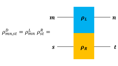
with ρm​n,s​tD=ρm​n​ρs​tsubscriptsuperscriptπœŒπ·π‘šπ‘›π‘ π‘‘subscriptπœŒπ‘šπ‘›subscriptπœŒπ‘ π‘‘\rho^{D}_{mn,st}=\rho_{mn}\rho_{st}. Here, we assume that the initial double space density matrix is the direct product of two same single space density matrices. ρDsuperscript𝜌𝐷\rho^{D} is illustrated in the Fig.Β (4).

Refer to caption
Figure 4: The schematic diagram of the definition of ρDsuperscript𝜌𝐷\rho^{D}.

Appendix B Three different definitions of entanglement entropy in the measurement-induced phase transition

In the evolution process together with measurements, measurements will produce different results. Thus, the density matrix in this process is the summation of the density matrix corresponding to the different measurement results, and each weight of the sum is the probability of that result. Therefore, we can write the density matrix as ρ=βˆ‘cpc​ρc𝜌subscript𝑐subscript𝑝𝑐subscriptπœŒπ‘\rho=\sum_{c}p_{c}\rho_{c}. Here, c𝑐c represents the different cases of evolution due to different measurement results. If we calculate the entanglement entropy directly from this mixed state density matrix, we obtain

Stotal=βˆ’log⁑{Tr​[(βˆ‘cpc​ρc)2]}.superscript𝑆totalTrdelimited-[]superscriptsubscript𝑐subscript𝑝𝑐subscriptπœŒπ‘2S^{\text{total}}=-\log\left\{\mathrm{Tr}\left[(\sum_{c}p_{c}\rho_{c})^{2}\right]\right\}. (26)

Also, we propose a new definition of the second-order RΓ©nyi entropy in our paper:

Snew=βˆ’log⁑{βˆ‘cpc~​Tr​[ρc2]}.superscript𝑆newsubscript𝑐~subscript𝑝𝑐Trdelimited-[]superscriptsubscriptπœŒπ‘2S^{\text{new}}=-\log\left\{\sum_{c}\tilde{p_{c}}\mathrm{Tr}[\rho_{c}^{2}]\right\}. (27)

Here, pc~=pc2βˆ‘cβ€²pcβ€²2~subscript𝑝𝑐superscriptsubscript𝑝𝑐2subscriptsuperscript𝑐′superscriptsubscript𝑝superscript𝑐′2\tilde{p_{c}}=\frac{p_{c}^{2}}{\sum_{c^{\prime}}p_{c^{\prime}}^{2}}. There is also another kind of the second-order RΓ©nyi entropy that people have used in the MIPT [8, 10]:

Sold=βˆ’βˆ‘cpc​log⁑{Tr​[ρc2]}.superscript𝑆oldsubscript𝑐subscript𝑝𝑐Trdelimited-[]superscriptsubscriptπœŒπ‘2S^{\text{old}}=-\sum_{c}p_{c}\log\{\mathrm{Tr}[\rho_{c}^{2}]\}. (28)

Appendix C The comparison of three different definitions of entanglement entropy in the MIPT

The entropy in MIPT comes from two parts: the entropy of the system corresponding to different measurement results βˆ’log⁑{Tr​[ρc2]}Trdelimited-[]superscriptsubscriptπœŒπ‘2-\log\{\text{Tr}[\rho_{c}^{2}]\}, and the entropy of the probability distribution of different measurement results {pc}subscript𝑝𝑐\{p_{c}\}. In the MIPT, we only care about the former part of entropy, and therefore we need to exclude the latter part.

We will show that both the Snewsuperscript𝑆newS^{\text{new}} and Soldsuperscript𝑆oldS^{\text{old}} can exclude the latter part of entropy, whereas Stotalsuperscript𝑆totalS^{\text{total}} can not. For instance, we assume that the system after evolution has a probability pcsubscript𝑝𝑐p_{c} to be in the case c𝑐c, and the density matrix in the case c𝑐c is ρcsubscriptπœŒπ‘\rho_{c}. Here, βˆ€c,pc>0for-all𝑐subscript𝑝𝑐0\forall c,p_{c}>0, and βˆ‘c=1npc=1​ with ​n>1superscriptsubscript𝑐1𝑛subscript𝑝𝑐1Β with 𝑛1\sum_{c=1}^{n}p_{c}=1\text{ with }n>1. We assume that every ρcsubscriptπœŒπ‘\rho_{c} satisfies Tr​[ρc2]=1Trdelimited-[]superscriptsubscriptπœŒπ‘21\mathrm{Tr}[\rho_{c}^{2}]=1, and this means that in each case, ρcsubscriptπœŒπ‘\rho_{c} is a pure state density matrix. Meanwhile, we assume Tr​(ρc​ρcβ€²)<1TrsubscriptπœŒπ‘subscript𝜌superscript𝑐′1\mathrm{Tr}(\rho_{c}\rho_{c^{\prime}})<1 for cβ‰ c′𝑐superscript𝑐′c\neq c^{\prime}, and this means ρcsubscriptπœŒπ‘\rho_{c} and ρcβ€²subscript𝜌superscript𝑐′\rho_{c^{\prime}} are not the same. Thus, the entropy only comes from the probability distribution {pc}={p1,p2,…,pn}subscript𝑝𝑐subscript𝑝1subscript𝑝2…subscript𝑝𝑛\{p_{c}\}=\{p_{1},p_{2},...,p_{n}\}. From the definition in the Eq.Β (26), we have

Stotal=superscript𝑆totalabsent\displaystyle S^{\text{total}}= βˆ’log⁑{Tr​[(βˆ‘c=1npc​ρc)2]}Trdelimited-[]superscriptsuperscriptsubscript𝑐1𝑛subscript𝑝𝑐subscriptπœŒπ‘2\displaystyle-\log\{\mathrm{Tr}[(\sum_{c=1}^{n}p_{c}\rho_{c})^{2}]\} (29)
=\displaystyle= βˆ’log⁑[βˆ‘c=1npc2​Tr​(ρc2)+2β€‹βˆ‘c<cβ€²pc​pc′​Tr​(ρc​ρcβ€²)]superscriptsubscript𝑐1𝑛superscriptsubscript𝑝𝑐2TrsuperscriptsubscriptπœŒπ‘22subscript𝑐superscript𝑐′subscript𝑝𝑐subscript𝑝superscript𝑐′TrsubscriptπœŒπ‘subscript𝜌superscript𝑐′\displaystyle-\log\left[\sum_{c=1}^{n}p_{c}^{2}\mathrm{Tr}(\rho_{c}^{2})+2\sum_{c<c^{\prime}}p_{c}p_{c^{\prime}}\mathrm{Tr}(\rho_{c}\rho_{c^{\prime}})\right]
>\displaystyle> βˆ’log⁑[βˆ‘c=1npc2​Tr​(ρc2)+2β€‹βˆ‘c<cβ€²pc​pcβ€²]superscriptsubscript𝑐1𝑛superscriptsubscript𝑝𝑐2TrsuperscriptsubscriptπœŒπ‘22subscript𝑐superscript𝑐′subscript𝑝𝑐subscript𝑝superscript𝑐′\displaystyle-\log\left[\sum_{c=1}^{n}p_{c}^{2}\mathrm{Tr}(\rho_{c}^{2})+2\sum_{c<c^{\prime}}p_{c}p_{c^{\prime}}\right]
=\displaystyle= βˆ’log⁑[βˆ‘c=1npc2+2β€‹βˆ‘c<cβ€²pc​pcβ€²]superscriptsubscript𝑐1𝑛superscriptsubscript𝑝𝑐22subscript𝑐superscript𝑐′subscript𝑝𝑐subscript𝑝superscript𝑐′\displaystyle-\log\left[\sum_{c=1}^{n}p_{c}^{2}+2\sum_{c<c^{\prime}}p_{c}p_{c^{\prime}}\right]
=\displaystyle= βˆ’log⁑[(βˆ‘c=1npc)2]=0.superscriptsuperscriptsubscript𝑐1𝑛subscript𝑝𝑐20\displaystyle-\log\left[(\sum_{c=1}^{n}p_{c})^{2}\right]=0.

Here, we use Tr​(ρA,c​ρA,cβ€²)<1TrsubscriptπœŒπ΄π‘subscript𝜌𝐴superscript𝑐′1\mathrm{Tr}(\rho_{A,c}\rho_{A,c^{\prime}})<1 for cβ‰ c′𝑐superscript𝑐′c\neq c^{\prime} to get the first inequality. Thus, we obtain Stotal>0superscript𝑆total0S^{\text{total}}>0.

In comparison with Stotalsuperscript𝑆totalS^{\text{total}}, from the definition in the Eq.Β (27), we have Snew=βˆ’log⁑[βˆ‘ipi~​Tr​(1)]=0superscript𝑆newsubscript𝑖~subscript𝑝𝑖Tr10S^{\text{new}}=-\log[\sum_{i}\tilde{p_{i}}\mathrm{Tr}(1)]=0. Also, from the definition in the Eq.Β (28), we have Sold=βˆ’βˆ‘ipi​log⁑[Tr​(1)]=0superscript𝑆oldsubscript𝑖subscript𝑝𝑖Tr10S^{\text{old}}=-\sum_{i}p_{i}\log[\mathrm{Tr}(1)]=0. Therefore, we find that Stotalsuperscript𝑆totalS^{\text{total}} takes into account the entropy of probability distribution {pc}={p1,p2,…,pn}subscript𝑝𝑐subscript𝑝1subscript𝑝2…subscript𝑝𝑛\{p_{c}\}=\{p_{1},p_{2},...,p_{n}\}, whereas Snewsuperscript𝑆newS^{\text{new}} and Soldsuperscript𝑆oldS^{\text{old}} do not.

Also, we find that if the density matrix in each case has the same purity and occurs with the same probability, then Snewsuperscript𝑆newS^{\text{new}} and Soldsuperscript𝑆oldS^{\text{old}} are the same. In this case, we have pc=1n,Tr​[ρc2]=aformulae-sequencesubscript𝑝𝑐1𝑛Trdelimited-[]superscriptsubscriptπœŒπ‘2π‘Žp_{c}=\frac{1}{n},\mathrm{Tr}[\rho_{c}^{2}]=a for c=1,…,n𝑐1…𝑛c=1,...,n. Then, we have Snew=βˆ’log⁑(βˆ‘c=1n1n​a)=βˆ’log⁑(a)superscript𝑆newsuperscriptsubscript𝑐1𝑛1π‘›π‘Žπ‘ŽS^{\text{new}}=-\log(\sum_{c=1}^{n}\frac{1}{n}a)=-\log(a), and Sold=βˆ’βˆ‘c=1n1n​log⁑a=βˆ’log⁑[a(nΓ—1n)]=βˆ’log⁑(a)superscript𝑆oldsuperscriptsubscript𝑐1𝑛1π‘›π‘Žsuperscriptπ‘Žπ‘›1π‘›π‘ŽS^{\text{old}}=-\sum_{c=1}^{n}\frac{1}{n}\log a=-\log[a^{(n\times\frac{1}{n})}]=-\log(a). Thus, we find that Snewsuperscript𝑆newS^{\text{new}} and Soldsuperscript𝑆oldS^{\text{old}} are the same in this case.

Appendix D The proof of an inequality between Stotalsuperscript𝑆totalS^{\text{total}} and Snewsuperscript𝑆newS^{\text{new}}

In this section, we will prove that when all density matrix ρcsubscriptπœŒπ‘\rho_{c} are mutually orthogonal, we have Stotalβ‰₯Snewsuperscript𝑆totalsuperscript𝑆newS^{\text{total}}\geq S^{\text{new}} where the equality is taken when there is only one outcome with probability p1=1subscript𝑝11p_{1}=1. Start from the definition Stotalsuperscript𝑆totalS^{\text{total}}, we have

Stotal=superscript𝑆totalabsent\displaystyle S^{\text{total}}= βˆ’log⁑{Tr​[(βˆ‘c=1npc​ρc)2]}Trdelimited-[]superscriptsuperscriptsubscript𝑐1𝑛subscript𝑝𝑐subscriptπœŒπ‘2\displaystyle-\log\{\mathrm{Tr}[(\sum_{c=1}^{n}p_{c}\rho_{c})^{2}]\} (30)
=\displaystyle= βˆ’log⁑[βˆ‘c,cβ€²=1npc​pc′​Tr​(ρc​ρcβ€²)]superscriptsubscript𝑐superscript𝑐′1𝑛subscript𝑝𝑐subscript𝑝superscript𝑐′TrsubscriptπœŒπ‘subscript𝜌superscript𝑐′\displaystyle-\log\left[\sum_{c,c^{\prime}=1}^{n}p_{c}p_{c^{\prime}}\mathrm{Tr}(\rho_{c}\rho_{c^{\prime}})\right]
=\displaystyle= βˆ’log⁑[βˆ‘cnpc2​Tr​(ρc2)]superscriptsubscript𝑐𝑛superscriptsubscript𝑝𝑐2TrsuperscriptsubscriptπœŒπ‘2\displaystyle-\log\left[\sum_{c}^{n}p_{c}^{2}\mathrm{Tr}(\rho_{c}^{2})\right]
β‰₯\displaystyle\geq βˆ’log⁑[βˆ‘cnpc~​Tr​(ρc2)]superscriptsubscript𝑐𝑛~subscript𝑝𝑐TrsuperscriptsubscriptπœŒπ‘2\displaystyle-\log\left[\sum_{c}^{n}\tilde{p_{c}}\mathrm{Tr}(\rho_{c}^{2})\right]
=\displaystyle= Snew.superscript𝑆new\displaystyle S^{\text{new}}.

Here, we use the Tr​(ρc​ρcβ€²)=0TrsubscriptπœŒπ‘subscript𝜌superscript𝑐′0\mathrm{Tr}(\rho_{c}\rho_{c^{\prime}})=0 for cβ‰ c′𝑐superscript𝑐′c\neq c^{\prime} to obtain the third equality. Here, Also, we use pc~=pc2βˆ‘cβ€²pcβ€²2β‰₯pc2~subscript𝑝𝑐superscriptsubscript𝑝𝑐2subscriptsuperscript𝑐′superscriptsubscript𝑝superscript𝑐′2superscriptsubscript𝑝𝑐2\tilde{p_{c}}=\frac{p_{c}^{2}}{\sum_{c^{\prime}}p_{c^{\prime}}^{2}}\geq p_{c}^{2} to obtain the fourth line. The equality in the fourth line is taken when there is only one outcome with probability p1=1subscript𝑝11p_{1}=1. Thus, we complete the proof.

Appendix E The quantum trajectories method

In this section, we introduce the quantum trajectories method regarding our generalized Lindblad equation the Eq.Β (18). The quantum trajectories method involves rewriting the master equation as a stochastic average over individual trajectories. It is an efficient tool for numerically simulating dissipative dynamics. Similar to the original Lindblad Master equation, our generalized Lindblad equation can be expressed in an alternative form:

βˆ‚ΟDβˆ‚t=βˆ’i​(H^effD​ρ​(t)βˆ’Οβ€‹(t)​H^effD⁣†)+η​(t)β€‹βˆ‘a=1nL^a,L​L^a,R​ρD​(t)​L^a,L†​L^a,R†Tr​(βˆ‘b=1nL^b,L​L^b,R​ρD​(t)​L^b,L†​L^b,R†).superscriptπœŒπ·π‘‘π‘–subscriptsuperscript^𝐻𝐷effπœŒπ‘‘πœŒπ‘‘subscriptsuperscript^𝐻𝐷†effπœ‚π‘‘superscriptsubscriptπ‘Ž1𝑛subscript^πΏπ‘ŽπΏsubscript^πΏπ‘Žπ‘…superscriptπœŒπ·π‘‘superscriptsubscript^πΏπ‘ŽπΏβ€ superscriptsubscript^πΏπ‘Žπ‘…β€ Trsuperscriptsubscript𝑏1𝑛subscript^𝐿𝑏𝐿subscript^𝐿𝑏𝑅superscriptπœŒπ·π‘‘superscriptsubscript^𝐿𝑏𝐿†superscriptsubscript^𝐿𝑏𝑅†\frac{\partial\rho^{D}}{\partial t}=-i\left(\hat{H}^{D}_{\text{eff}}\rho(t)-\rho(t)\hat{H}^{D\dagger}_{\text{eff}}\right)+\eta(t)\sum_{a=1}^{n}\frac{\hat{L}_{a,L}\hat{L}_{a,R}\rho^{D}(t)\hat{L}_{a,L}^{\dagger}\hat{L}_{a,R}^{\dagger}}{\mathrm{Tr}\left(\sum_{b=1}^{n}\hat{L}_{b,L}\hat{L}_{b,R}\rho^{D}(t)\hat{L}_{b,L}^{\dagger}\hat{L}_{b,R}^{\dagger}\right)}. (31)

Here H^effDsubscriptsuperscript^𝐻𝐷eff\hat{H}^{D}_{\text{eff}} is the effective Hamiltonian defined as

H^effD=H^βŠ—I^+I^βŠ—H^βˆ’i​η​(t)2β€‹βˆ‘a,bL^a,L†​L^a,L​L^b,R†​L^b,R.subscriptsuperscript^𝐻𝐷efftensor-product^𝐻^𝐼tensor-product^𝐼^π»π‘–πœ‚π‘‘2subscriptπ‘Žπ‘superscriptsubscript^πΏπ‘ŽπΏβ€ subscript^πΏπ‘ŽπΏsuperscriptsubscript^𝐿𝑏𝑅†subscript^𝐿𝑏𝑅\displaystyle\hat{H}^{D}_{\text{eff}}=\hat{H}\otimes\hat{I}+\hat{I}\otimes\hat{H}-i\frac{\eta(t)}{2}\sum_{a,b}\hat{L}_{a,L}^{\dagger}\hat{L}_{a,L}\hat{L}_{b,R}^{\dagger}\hat{L}_{b,R}. (32)

First, we start from a double system initial state |Ο•D​(t)⟩ketsuperscriptitalic-ϕ𝐷𝑑|\phi^{D}(t)\rangle, and compute its evolution under the effective Hamiltonian after a small time-step δ​t𝛿𝑑\delta t:

|Ο•(1),D​(t+δ​t)⟩=(1βˆ’i​HeffD​δ​t)​|Ο•D​(t)⟩.ketsuperscriptitalic-Ο•1𝐷𝑑𝛿𝑑1𝑖superscriptsubscript𝐻eff𝐷𝛿𝑑ketsuperscriptitalic-ϕ𝐷𝑑|\phi^{(1),D}(t+\delta t)\rangle=(1-iH_{\text{eff}}^{D}\delta t)|\phi^{D}(t)\rangle. (33)

Then, we compute the norm of this wave function at time t+δ​t𝑑𝛿𝑑t+\delta t.

βŸ¨Ο•(1),D​(t+δ​t)|Ο•(1),D​(t+δ​t)βŸ©β‰‘1βˆ’Ξ΄β€‹pinner-productsuperscriptitalic-Ο•1𝐷𝑑𝛿𝑑superscriptitalic-Ο•1𝐷𝑑𝛿𝑑1𝛿𝑝\langle\phi^{(1),D}(t+\delta t)|\phi^{(1),D}(t+\delta t)\rangle\equiv 1-\delta p (34)

where

δ​p=η​(t)β€‹βŸ¨Ο•D​(t)|i​(HeffDβˆ’HeffD⁣†)|Ο•D​(t)βŸ©β€‹Ξ΄β€‹t=η​(t)β€‹βŸ¨Ο•D​(t)|βˆ‘a,bL^a,L†​L^a,L​L^b,R†​L^b,R|Ο•D​(t)βŸ©β€‹Ξ΄β€‹t.π›Ώπ‘πœ‚π‘‘quantum-operator-productsuperscriptitalic-ϕ𝐷𝑑𝑖superscriptsubscript𝐻eff𝐷superscriptsubscript𝐻eff𝐷†superscriptitalic-Ο•π·π‘‘π›Ώπ‘‘πœ‚π‘‘quantum-operator-productsuperscriptitalic-ϕ𝐷𝑑subscriptπ‘Žπ‘superscriptsubscript^πΏπ‘ŽπΏβ€ subscript^πΏπ‘ŽπΏsuperscriptsubscript^𝐿𝑏𝑅†subscript^𝐿𝑏𝑅superscriptitalic-ϕ𝐷𝑑𝛿𝑑\delta p=\eta(t)\langle\phi^{D}(t)|i(H_{\text{eff}}^{D}-H_{\text{eff}}^{D\dagger})|\phi^{D}(t)\rangle\delta t=\eta(t)\langle\phi^{D}(t)|\sum_{a,b}\hat{L}_{a,L}^{\dagger}\hat{L}_{a,L}\hat{L}_{b,R}^{\dagger}\hat{L}_{b,R}|\phi^{D}(t)\rangle\delta t. (35)

Here, we assume the completeness condition of Eq.Β (5). Thus, we further have

δ​p=η​(t)​δ​t.π›Ώπ‘πœ‚π‘‘π›Ώπ‘‘\delta p=\eta(t)\delta t. (36)

Second, we choose the propagated state stochastically in the following manner:
1. With probability 1βˆ’Ξ΄β€‹p1𝛿𝑝1-\delta p, the wave function at t+δ​t𝑑𝛿𝑑t+\delta t is chosen as the one that evolves under the effective Hamiltonian with a normalization factor accordingly:

|Ο•D​(t+δ​t)⟩=|Ο•(1),D​(t+δ​t)⟩1βˆ’Ξ΄β€‹p.ketsuperscriptitalic-ϕ𝐷𝑑𝛿𝑑ketsuperscriptitalic-Ο•1𝐷𝑑𝛿𝑑1𝛿𝑝|\phi^{D}(t+\delta t)\rangle=\frac{|\phi^{(1),D}(t+\delta t)\rangle}{\sqrt{1-\delta p}}. (37)

2. With probability δ​p𝛿𝑝\delta p, the wave function at t+δ​t𝑑𝛿𝑑t+\delta t is chosen as the one that jumps to some particular quantum channel aπ‘Ža:

|Ο•D​(t+δ​t)⟩=L^a,L​L^a,R​|Ο•D​(t)βŸ©Ξ΄β€‹paδ​tketsuperscriptitalic-ϕ𝐷𝑑𝛿𝑑subscript^πΏπ‘ŽπΏsubscript^πΏπ‘Žπ‘…ketsuperscriptitalic-ϕ𝐷𝑑𝛿subscriptπ‘π‘Žπ›Ώπ‘‘|\phi^{D}(t+\delta t)\rangle=\frac{\hat{L}_{a,L}\hat{L}_{a,R}|\phi^{D}(t)\rangle}{\sqrt{\frac{\delta p_{a}}{\delta t}}} (38)

where δ​pa=δ​tβ€‹βŸ¨Ο•D​(t)|L^a,R†​L^a,L†​L^a,L​L^a,R|Ο•D​(t)βŸ©π›Ώsubscriptπ‘π‘Žπ›Ώπ‘‘quantum-operator-productsuperscriptitalic-ϕ𝐷𝑑superscriptsubscript^πΏπ‘Žπ‘…β€ superscriptsubscript^πΏπ‘ŽπΏβ€ subscript^πΏπ‘ŽπΏsubscript^πΏπ‘Žπ‘…superscriptitalic-ϕ𝐷𝑑\delta p_{a}=\delta t\langle\phi^{D}(t)|\hat{L}_{a,R}^{\dagger}\hat{L}_{a,L}^{\dagger}\hat{L}_{a,L}\hat{L}_{a,R}|\phi^{D}(t)\rangle. Here, each quantum channel aπ‘Ža is chosen with a probability Ξ a=δ​paβˆ‘bδ​pb​δ​psubscriptΞ π‘Žπ›Ώsubscriptπ‘π‘Žsubscript𝑏𝛿subscript𝑝𝑏𝛿𝑝\Pi_{a}=\frac{\delta p_{a}}{\sum_{b}\delta p_{b}}\delta p.

Since from the prescription above, the propagation of the initial density matrix ρD​(t)=|Ο•D​(t)βŸ©β€‹βŸ¨Ο•D​(t)|superscriptπœŒπ·π‘‘ketsuperscriptitalic-ϕ𝐷𝑑brasuperscriptitalic-ϕ𝐷𝑑\rho^{D}(t)=|\phi^{D}(t)\rangle\langle\phi^{D}(t)| in a given time step is:

ρD​(t+δ​t)Β―=Β―superscriptπœŒπ·π‘‘π›Ώπ‘‘absent\displaystyle\overline{\rho^{D}(t+\delta t)}= (1βˆ’Ξ΄β€‹p)​|Ο•(1),D​(t+δ​t)⟩1βˆ’Ξ΄β€‹pβ€‹βŸ¨Ο•(1),D​(t+δ​t)|1βˆ’Ξ΄β€‹p+δ​pβ€‹βˆ‘aΞ a​L^a,L​L^a,R​|Ο•D​(t)βŸ©Ξ΄β€‹paδ​tβ€‹βŸ¨Ο•D​(t)|​L^a,R†​L^a,L†δ​paδ​t1𝛿𝑝ketsuperscriptitalic-Ο•1𝐷𝑑𝛿𝑑1𝛿𝑝brasuperscriptitalic-Ο•1𝐷𝑑𝛿𝑑1𝛿𝑝𝛿𝑝subscriptπ‘ŽsubscriptΞ π‘Žsubscript^πΏπ‘ŽπΏsubscript^πΏπ‘Žπ‘…ketsuperscriptitalic-ϕ𝐷𝑑𝛿subscriptπ‘π‘Žπ›Ώπ‘‘brasuperscriptitalic-ϕ𝐷𝑑superscriptsubscript^πΏπ‘Žπ‘…β€ superscriptsubscript^πΏπ‘ŽπΏβ€ π›Ώsubscriptπ‘π‘Žπ›Ώπ‘‘\displaystyle(1-\delta p)\frac{|\phi^{(1),D}(t+\delta t)\rangle}{\sqrt{1-\delta p}}\frac{\langle\phi^{(1),D}(t+\delta t)|}{\sqrt{1-\delta p}}+\delta p\sum_{a}\Pi_{a}\frac{\hat{L}_{a,L}\hat{L}_{a,R}|\phi^{D}(t)\rangle}{\sqrt{\frac{\delta p_{a}}{\delta t}}}\frac{\langle\phi^{D}(t)|\hat{L}_{a,R}^{\dagger}\hat{L}_{a,L}^{\dagger}}{\sqrt{\frac{\delta p_{a}}{\delta t}}} (39)
=\displaystyle= |Ο•(1),D​(t+δ​t)βŸ©β€‹βŸ¨Ο•(1),D​(t+δ​t)|+η​(t)​δ​tβ€‹βˆ‘aL^a,L​L^a,R​|Ο•D​(t)βŸ©β€‹βŸ¨Ο•D​(t)|​L^a,R†​L^a,L†Tr​(βˆ‘b=1nL^b,L​L^b,R​ρD​(t)​L^b,L†​L^b,R†)ketsuperscriptitalic-Ο•1𝐷𝑑𝛿𝑑brasuperscriptitalic-Ο•1π·π‘‘π›Ώπ‘‘πœ‚π‘‘π›Ώπ‘‘subscriptπ‘Žsubscript^πΏπ‘ŽπΏsubscript^πΏπ‘Žπ‘…ketsuperscriptitalic-ϕ𝐷𝑑brasuperscriptitalic-ϕ𝐷𝑑superscriptsubscript^πΏπ‘Žπ‘…β€ superscriptsubscript^πΏπ‘ŽπΏβ€ Trsuperscriptsubscript𝑏1𝑛subscript^𝐿𝑏𝐿subscript^𝐿𝑏𝑅superscriptπœŒπ·π‘‘superscriptsubscript^𝐿𝑏𝐿†superscriptsubscript^𝐿𝑏𝑅†\displaystyle|\phi^{(1),D}(t+\delta t)\rangle\langle\phi^{(1),D}(t+\delta t)|+\eta(t)\delta t\sum_{a}\frac{\hat{L}_{a,L}\hat{L}_{a,R}|\phi^{D}(t)\rangle\langle\phi^{D}(t)|\hat{L}_{a,R}^{\dagger}\hat{L}_{a,L}^{\dagger}}{\mathrm{Tr}\left(\sum_{b=1}^{n}\hat{L}_{b,L}\hat{L}_{b,R}\rho^{D}(t)\hat{L}_{b,L}^{\dagger}\hat{L}_{b,R}^{\dagger}\right)}
=\displaystyle= βˆ’i​(H^effD​ρ​(t)βˆ’Οβ€‹(t)​H^effD⁣†)​δ​t+η​(t)​δ​tβ€‹βˆ‘aL^a,L​L^a,R​|Ο•D​(t)βŸ©β€‹βŸ¨Ο•D​(t)|​L^a,R†​L^a,L†Tr​(βˆ‘b=1nL^b,L​L^b,R​ρD​(t)​L^b,L†​L^b,R†).𝑖subscriptsuperscript^𝐻𝐷effπœŒπ‘‘πœŒπ‘‘subscriptsuperscript^𝐻𝐷†effπ›Ώπ‘‘πœ‚π‘‘π›Ώπ‘‘subscriptπ‘Žsubscript^πΏπ‘ŽπΏsubscript^πΏπ‘Žπ‘…ketsuperscriptitalic-ϕ𝐷𝑑brasuperscriptitalic-ϕ𝐷𝑑superscriptsubscript^πΏπ‘Žπ‘…β€ superscriptsubscript^πΏπ‘ŽπΏβ€ Trsuperscriptsubscript𝑏1𝑛subscript^𝐿𝑏𝐿subscript^𝐿𝑏𝑅superscriptπœŒπ·π‘‘superscriptsubscript^𝐿𝑏𝐿†superscriptsubscript^𝐿𝑏𝑅†\displaystyle-i\left(\hat{H}^{D}_{\text{eff}}\rho(t)-\rho(t)\hat{H}^{D\dagger}_{\text{eff}}\right)\delta t+\eta(t)\delta t\sum_{a}\frac{\hat{L}_{a,L}\hat{L}_{a,R}|\phi^{D}(t)\rangle\langle\phi^{D}(t)|\hat{L}_{a,R}^{\dagger}\hat{L}_{a,L}^{\dagger}}{\mathrm{Tr}\left(\sum_{b=1}^{n}\hat{L}_{b,L}\hat{L}_{b,R}\rho^{D}(t)\hat{L}_{b,L}^{\dagger}\hat{L}_{b,R}^{\dagger}\right)}.

Here, the ρD​(t+δ​t)Β―Β―superscriptπœŒπ·π‘‘π›Ώπ‘‘\overline{\rho^{D}(t+\delta t)} denotes a statistical average over trajectories. It is straightforward to see that the stochastic propagation given by this quantum trajectories method is equivalent to our generalized Lindblad equation Eq.Β (18) after taking a stochastic average over trajectories.
We use this quantum trajectories method to numerically calculate the half-system entanglement entropy in a larger system size similar to Fig.Β 2 and Fig.Β 3. Also, since we are calculating the entropy using the wave function of the double system whose dimension of the Hilbert space is the square of that of the single system, the total single system size that we can simulate efficiently is therefore limited. Here, we calculate the half-system entanglement entropy at total system size L=2,4,6,8𝐿2468L=2,4,6,8 and the dissipation strength Ξ³=0.5,1,3,4𝛾0.5134\gamma=0.5,1,3,4 using this quantum trajectories method, and the average longtime saturation entanglement entropy is shown in Fig.Β 5.

Refer to caption
Figure 5: The longtime saturation value of entanglement entropy SAsubscript𝑆𝐴S_{A} of the subsystem A𝐴A with different system size Nssubscript𝑁𝑠N_{s} and fixing LA=L/4subscript𝐿𝐴𝐿4L_{A}=L/4, total number of bosons Nb=L/2subscript𝑁𝑏𝐿2N_{b}=L/2. Different curves have different γ𝛾\gamma in the unit of J𝐽J. Here, U/J=1π‘ˆπ½1U/J=1. We choose a set of N=100𝑁100N=100 quantum trajectories for L=8𝐿8L=8 and N=1000𝑁1000N=1000 quantum trajectories for L=2,4,6𝐿246L=2,4,6.We choose the initial state as a product state in the particle number basis. We choose the initial state |01⟩ket01|01\rangle for L=2, |0011⟩ket0011|0011\rangle for L=4, |000111⟩ket000111|000111\rangle for L=6 and |00001111⟩ket00001111|00001111\rangle for L=8.

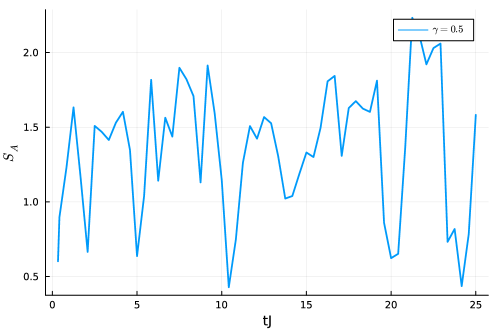
For small values of γ𝛾\gamma (Ξ³/J=0.5𝛾𝐽0.5\gamma/J=0.5), we see an almost linear growth in the entanglement entropy as the total system size increases, which indicates that there could be a volume-low scaling at a larger system size. In comparison, for large values of γ𝛾\gamma (Ξ³/J=4𝛾𝐽4\gamma/J=4), we see a seemly logarithmic growth in the entanglement entropy as the total system size increases, which indicates that there could be a logarithmic critical scaling or an area law (constant) scaling at a larger system size. Also, this result is in line with the understanding that there could be an entanglement phase transition in this process. Also, we illustrate the entanglement entropy computed on a single realization of a quantum trajectory in Fig.Β 6. and Fig.Β 7.

Refer to caption
Figure 6: The entanglement entropy computed on the single realization of a quantum trajectory. Here, U=Jπ‘ˆπ½U=J and the number of sites Ns=6subscript𝑁𝑠6N_{s}=6, and the number of bosons Nb=3subscript𝑁𝑏3N_{b}=3, and subsystem size LA=3subscript𝐿𝐴3L_{A}=3. The measurement rate is Ξ³/J=0.5𝛾𝐽0.5\gamma/J=0.5.
Refer to caption
Figure 7: The entanglement entropy computed on the single realization of a quantum trajectory. Here, U=Jπ‘ˆπ½U=J and the number of sites Ns=6subscript𝑁𝑠6N_{s}=6, and the number of bosons Nb=3subscript𝑁𝑏3N_{b}=3, and subsystem size LA=3subscript𝐿𝐴3L_{A}=3. The measurement rate is Ξ³/J=1.5𝛾𝐽1.5\gamma/J=1.5.

The average number of measurements in our simulation is

Nm​e​a​n=Tt​o​t​a​ld​t​L​γ​d​t=Tt​o​t​a​l​L​γ.subscriptπ‘π‘šπ‘’π‘Žπ‘›subscriptπ‘‡π‘‘π‘œπ‘‘π‘Žπ‘™π‘‘π‘‘πΏπ›Ύπ‘‘π‘‘subscriptπ‘‡π‘‘π‘œπ‘‘π‘Žπ‘™πΏπ›ΎN_{mean}=\frac{T_{total}}{dt}L\gamma dt=T_{total}L\gamma. (40)

For instance, in our simulations, Tt​o​t​a​l=30,L=8,Ξ³=1formulae-sequencesubscriptπ‘‡π‘‘π‘œπ‘‘π‘Žπ‘™30formulae-sequence𝐿8𝛾1T_{total}=30,L=8,\gamma=1, each realization of the stochastic protocol consists of Nm​e​a​n=240subscriptπ‘π‘šπ‘’π‘Žπ‘›240N_{mean}=240 projective measurements on average. Here, we chose a set of N=100𝑁100N=100 quantum trajectories for L=8𝐿8L=8 and N=1000𝑁1000N=1000 quantum trajectories for L=2,4,6𝐿246L=2,4,6.

Appendix F The entanglement entropy of complement subsystems

In this section, we will prove that the entanglement entropy calculated from the entropy formula the Eq. (17) for the evolved density matrix the Eq. (18) is the same regardless of whether one computes partial trace over the subsystem A𝐴A or subsystem B𝐡B. Here, subsystems A𝐴A and B𝐡B are complement subsystems of the total system. From the Eq. (22), we have

SAD=βˆ’log⁑{βˆ‘b=0mpb~​TrA​[ρA,b2]}.superscriptsubscript𝑆𝐴𝐷superscriptsubscript𝑏0π‘š~subscript𝑝𝑏subscriptTr𝐴delimited-[]superscriptsubscriptπœŒπ΄π‘2S_{A}^{D}=-\log\left\{\sum_{b=0}^{m}\tilde{p_{b}}\mathrm{Tr}_{A}\left[\rho_{A,b}^{2}\right]\right\}. (41)

Also, if we change the subsystem A𝐴A to its complement subsystem B, we have

SBD=βˆ’log⁑{βˆ‘b=0mpb~​TrB​[ρB,b2]}.superscriptsubscript𝑆𝐡𝐷superscriptsubscript𝑏0π‘š~subscript𝑝𝑏subscriptTr𝐡delimited-[]superscriptsubscriptπœŒπ΅π‘2S_{B}^{D}=-\log\left\{\sum_{b=0}^{m}\tilde{p_{b}}\mathrm{Tr}_{B}\left[\rho_{B,b}^{2}\right]\right\}. (42)

with pb~=[Tr​(M^b​ρ0​(t)​M^b†)]2~subscript𝑝𝑏superscriptdelimited-[]Trsubscript^𝑀𝑏subscript𝜌0𝑑superscriptsubscript^𝑀𝑏†2\tilde{p_{b}}=\left[\mathrm{Tr}\left(\hat{M}_{b}\rho_{0}(t)\hat{M}_{b}^{\dagger}\right)\right]^{2} and ρb=M^b​ρ0​(t)​M^b†Tr​(M^b​ρ0​(t)​M^b†)subscriptπœŒπ‘subscript^𝑀𝑏subscript𝜌0𝑑superscriptsubscript^𝑀𝑏†Trsubscript^𝑀𝑏subscript𝜌0𝑑superscriptsubscript^𝑀𝑏†\rho_{b}=\frac{\hat{M}_{b}\rho_{0}(t)\hat{M}_{b}^{\dagger}}{\mathrm{Tr}\left(\hat{M}_{b}\rho_{0}(t)\hat{M}_{b}^{\dagger}\right)}. Here, each ρbsubscriptπœŒπ‘\rho_{b} is pure if we start from a pure state. For a pure state density matrix, using the Schmidt decomposition, we can prove that TrA​[ρA,b2]=TrB​[ρB,b2]subscriptTr𝐴delimited-[]superscriptsubscriptπœŒπ΄π‘2subscriptTr𝐡delimited-[]superscriptsubscriptπœŒπ΅π‘2\mathrm{Tr}_{A}\left[\rho_{A,b}^{2}\right]=\mathrm{Tr}_{B}\left[\rho_{B,b}^{2}\right], thus we obtain

SBDsuperscriptsubscript𝑆𝐡𝐷\displaystyle S_{B}^{D} =βˆ’log⁑{βˆ‘b=0mpb~​TrB​[ρB,b2]}absentsuperscriptsubscript𝑏0π‘š~subscript𝑝𝑏subscriptTr𝐡delimited-[]superscriptsubscriptπœŒπ΅π‘2\displaystyle=-\log\left\{\sum_{b=0}^{m}\tilde{p_{b}}\mathrm{Tr}_{B}\left[\rho_{B,b}^{2}\right]\right\} (43)
=βˆ’log⁑{βˆ‘b=0mpb~​TrA​[ρA,b2]}absentsuperscriptsubscript𝑏0π‘š~subscript𝑝𝑏subscriptTr𝐴delimited-[]superscriptsubscriptπœŒπ΄π‘2\displaystyle=-\log\left\{\sum_{b=0}^{m}\tilde{p_{b}}\mathrm{Tr}_{A}\left[\rho_{A,b}^{2}\right]\right\}
=SAD.absentsuperscriptsubscript𝑆𝐴𝐷\displaystyle=S_{A}^{D}.

Appendix G Numerical results of the entropy computed from the single-copy master equation

In this section, we will give some numerical results about the system driven by the generalized Lindblad equation the Eq.Β (8) in the original single system, and we set η​(t)=Ξ³πœ‚π‘‘π›Ύ\eta(t)=\gamma as a time-independent measurement rate. Also, we set the projection measurements as

L^i,0=1L​(1βˆ’n^i),L^i,1=1L​n^i.formulae-sequencesubscript^𝐿𝑖01𝐿1subscript^𝑛𝑖subscript^𝐿𝑖11𝐿subscript^𝑛𝑖\hat{L}_{i,0}=\frac{1}{\sqrt{L}}(1-\hat{n}_{i}),\ \hat{L}_{i,1}=\frac{1}{\sqrt{L}}\hat{n}_{i}. (44)

The Hamiltonian of is also the hard-core Bose Hubbard system

H^=βˆ’Jβ€‹βˆ‘βŸ¨i,j⟩b^i†​b^j+Uβ€‹βˆ‘βŸ¨i,j⟩n^i​n^j.^𝐻𝐽subscript𝑖𝑗superscriptsubscript^𝑏𝑖†subscript^π‘π‘—π‘ˆsubscript𝑖𝑗subscript^𝑛𝑖subscript^𝑛𝑗\hat{H}=-J\sum_{\langle i,j\rangle}\hat{b}_{i}^{\dagger}\hat{b}_{j}+U\sum_{\langle i,j\rangle}\hat{n}_{i}\hat{n}_{j}. (45)

as the section 7 for comparison. Here, J𝐽J is the strength of the nearest neighbor hopping, and Uπ‘ˆU is the strength of the nearest neighbor interaction.

In our following numerical calculation, we set J=U=1,Ns=6,Nb=3formulae-sequenceπ½π‘ˆ1formulae-sequencesubscript𝑁𝑠6subscript𝑁𝑏3J=U=1,N_{s}=6,N_{b}=3. Nbsubscript𝑁𝑏N_{b} is the total number of the hard-core boson. We denote the left half of the system as subsystem A𝐴A and the rest of it as subsystem B𝐡B. We then calculate the entanglement entropy SAsubscript𝑆𝐴S_{A} defined in the Eq.Β (17). We choose the initial state as the a product state in the particle number basis |000111⟩ket000111|000111\rangle.

Refer to caption
Figure 8: The dynamics of the entanglement entropy SAsubscript𝑆𝐴S_{A} as a function of t​J𝑑𝐽tJ. γ𝛾\gamma is the measurement rate. Different curves have different γ𝛾\gamma in the unit of J𝐽J. Here, U=Jπ‘ˆπ½U=J and the number of sites Ns=6subscript𝑁𝑠6N_{s}=6, and the number of bosons Nb=3subscript𝑁𝑏3N_{b}=3, and subsystem size LA=3subscript𝐿𝐴3L_{A}=3. The density matrix is evolved by the single-copy master equation the Eq.Β (8).
Refer to caption
Figure 9: Saturation value of entanglement entropy SAsubscript𝑆𝐴S_{A} of the subsystem A𝐴A with different subsystem size LAsubscript𝐿𝐴L_{A}. Different curves have different γ𝛾\gamma in the unit of J𝐽J. Here, Ns=6subscript𝑁𝑠6N_{s}=6, Nb=3subscript𝑁𝑏3N_{b}=3, U/J=1π‘ˆπ½1U/J=1. The density matrix is evolved by the single-copy master equation the Eq.Β (8).

As shown in Fig.Β 8, the entanglement entropy SAsubscript𝑆𝐴S_{A} between subsystems A𝐴A and B𝐡B increases as expected in a normal chaotic system, and it then saturates to a non-zero value. However, compared with the dynamics of the entanglement entropy SAsubscript𝑆𝐴S_{A} in the Fig.Β 2, it does not decrease in this process, and the saturation value of SAsubscript𝑆𝐴S_{A} shown in the Fig.Β 9 is the same as measurement rate changes.

Therefore, we find that there is no entanglement phase transition in this process, and there is no surprise since we have mentioned in the section 5 that the entanglement entropy calculated from the single-copy master equation is SAtotalsubscriptsuperscript𝑆total𝐴S^{\text{total}}_{A} defined in the Eq.Β (14) as

SAtotalβ‰‘βˆ’log⁑{Tr​[(βˆ‘c=1mpc​ρA,c)2]}.subscriptsuperscript𝑆total𝐴Trdelimited-[]superscriptsuperscriptsubscript𝑐1π‘šsubscript𝑝𝑐subscriptπœŒπ΄π‘2S^{\text{total}}_{A}\equiv-\log\left\{\mathrm{Tr}\left[\left(\sum_{c=1}^{m}p_{c}\rho_{A,c}\right)^{2}\right]\right\}. (46)

Here, pcsubscript𝑝𝑐p_{c} is the probability of getting ρA,csubscriptπœŒπ΄π‘\rho_{A,c}, and it satisfies βˆ‘cpc=1subscript𝑐subscript𝑝𝑐1\sum_{c}p_{c}=1. Since SAtotalsubscriptsuperscript𝑆total𝐴S^{\text{total}}_{A} also includes the entropy corresponding to the probability distribution of different measurement results, there is no entanglement phase transition regarding this entanglement entropy.

Appendix H The detail information about the numerical integration technique used in producing Fig.Β 2 and Fig.Β 3

We used the Runge-Kutta 4th-order (RK4) method for the approximate solutions of simultaneous nonlinear equations about the double system density matrix. For the Fig.Β 2 and Fig.Β 3, we used Nt=11000subscript𝑁𝑑11000N_{t}=11000 time steps.

Appendix I The comparison between Eq.(6) with the assumption βˆ‘a=1nL^a†​L^a=ℐsuperscriptsubscriptπ‘Ž1𝑛superscriptsubscript^πΏπ‘Žβ€ subscript^πΏπ‘Žβ„\sum_{a=1}^{n}\hat{L}_{a}^{\dagger}\hat{L}_{a}=\mathcal{I} and the general Lindbald equation.

In deriving the Linblad-like equation in the section.Β (2), we assume that the measurement is performed on a complete basis, thus the anti-commutator part of the Lindblad master equation is trivial and amounts to an identity matrix. In general, the Lindblad master equation does not need to satisfy the Eq.Β (5). Thus, the equation we obtain with the condition Eq.Β (5) is a special case of the general Lindblad equation.
The method we have used here to derive this Lindblad-like equation is first evolving the system under unitary evolution and then doing projection according to the probability p​(t)𝑝𝑑p(t) on the system. The density matrix after this probabilistic measurement is:

ρM​(t+δ​t)=[1βˆ’P​(t+δ​t)]​ρ​(t+δ​t)+P​(t+δ​t)β€‹βˆ‘aL^a​ρ​(t+δ​t)​L^a†.superscriptπœŒπ‘€π‘‘π›Ώπ‘‘delimited-[]1π‘ƒπ‘‘π›Ώπ‘‘πœŒπ‘‘π›Ώπ‘‘π‘ƒπ‘‘π›Ώπ‘‘subscriptπ‘Žsubscript^πΏπ‘ŽπœŒπ‘‘π›Ώπ‘‘superscriptsubscript^πΏπ‘Žβ€ \rho^{M}(t+\delta t)=\left[1-P(t+\delta t)\right]\rho(t+\delta t)+P(t+\delta t)\sum_{a}\hat{L}_{a}\rho(t+\delta t)\hat{L}_{a}^{\dagger}. (47)

Here, the quantum jump terms βˆ‘a=1nL^a​ρ​(t)​L^a†superscriptsubscriptπ‘Ž1𝑛subscript^πΏπ‘ŽπœŒπ‘‘superscriptsubscript^πΏπ‘Žβ€ \sum_{a=1}^{n}\hat{L}_{a}\rho(t)\hat{L}_{a}^{\dagger} in the equation Eq.Β (6) totally comes from doing measurement on the system. Thus, doing projection on a complete basis directly leads to the condition Eq.Β (5). Also, this probabilistic measurement process in the Eq.Β (47) leads to the anti-commutator part of the Lindblad master equation coming from P​(t+δ​t)​ρ​(t+δ​t)π‘ƒπ‘‘π›Ώπ‘‘πœŒπ‘‘π›Ώπ‘‘P(t+\delta t)\rho(t+\delta t). Thus, the anti-commutator part amounts to an identity matrix. Also, if we do not assume this probabilistic measurement process in Eq.Β (47), the system under unitary evolution together with the measurement process can be described in other ways. For instance, by considering the system being driven by a non-hermitian Hamiltonian[31, 12], we normalize the quantum state after each step of this protocol. In these protocols,we have βˆ‘a=1nL^a†​L^a≠ℐsuperscriptsubscriptπ‘Ž1𝑛superscriptsubscript^πΏπ‘Žβ€ subscript^πΏπ‘Žβ„\sum_{a=1}^{n}\hat{L}_{a}^{\dagger}\hat{L}_{a}\neq\mathcal{I} in general.