A stochastic Stein variational Newton method

Abstract

Stein variational gradient descent (SVGD) is a general-purpose optimization-based sampling algorithm that has recently exploded in popularity, but is limited by two issues: it is known to produce biased samples, and it can be slow to converge on complicated distributions. A recently proposed stochastic variant of SVGD (sSVGD) addresses the first issue, producing unbiased samples by incorporating a special noise into the SVGD dynamics such that asymptotic convergence is guaranteed. Meanwhile, Stein variational Newton (SVN), a Newton-like extension of SVGD, dramatically accelerates the convergence of SVGD by incorporating Hessian information into the dynamics, but also produces biased samples. In this paper we derive, and provide a practical implementation of, a stochastic variant of SVN (sSVN) which is both asymptotically correct and converges rapidly. We demonstrate the effectiveness of our algorithm on a difficult class of test problems—the Hybrid Rosenbrock density—and show that sSVN converges using three orders of magnitude fewer gradient evaluations of the log likelihood than its stochastic SVGD counterpart. Our results show that sSVN is a promising approach to accelerating high-precision Bayesian inference tasks with modest-dimension, $d\sim\mathcal{O}(10)$.

1 Introduction

The goal of Bayesian inference in data analysis is to infer probability distributions (posteriors) for model parameters, given a dataset van de Schoot et al., (2021). It is a powerful framework for parameter estimation, but poses significant computational challenges. The posterior must generally be evaluated numerically and the parameter space may be high dimensional. Consequently, quantities of interest—such as moments and various other integrals of the posterior—are non-trivial to calculate.

Markov chain Monte Carlo (MCMC) is a widely used technique to approximate such integrals Speagle, (2020). By defining a suitable Markov chain, one may in principle draw i.i.d. samples from the posterior and thus calculate arbitrary integrals of the posterior with $\mathcal{O}(1/\sqrt{N})$ accuracy, where $N$ is the sample size drawn. In many applications however, MCMC algorithms may be unacceptably slow to converge.

Variational inference (VI), on the other hand, is a technique which trades accuracy for speed. VI algorithms approximate posterior integrals by solving an optimization problem Blei et al., (2017). A popular example of such an approach is Stein variational gradient descent (SVGD), which is a non-parametric VI algorithm which implements a form of functional gradient descent Liu and Wang, (2016). Likewise, Stein variational Newton (SVN) Detommaso et al., (2018); Chen et al., (2020) extends SVGD by implementing a form of functional Newton descent, dramatically accelerating convergence to the posterior at the price of additional work per iteration.

Although VI algorithms were originally developed to accelerate Bayesian inference in machine learning, many areas of science and engineering similarly rely on Bayesian inference, albiet with a modest number of dimensions $d\sim\mathcal{O}(10)$. This is the case, for example, in many astrophysical applications such as cosmology (e.g. Aghanim et al.,, 2020) and gravitational wave astronomy (e.g. Abbott et al.,, 2021). VI offers the possibility of significantly accelerating inference, and is thus a tempting candidate to investigate further Gunapati et al., (2018). However, the inexact nature of VI limits its utility: especially in fields where high-precision posterior sampling is required.

Ideally one would construct an algorithm with the speed and flexibility of VI, but with the asymptotic convergence gaurantees of MCMC. Indeed, an example of such an algorithm was proposed in Gallego and Insua, (2020), which showed that SVGD may be asymptotically corrected by adding in a special noise term, which leads to a stochastic SVGD (sSVGD) algorithm. Compared to naive MCMC algorithms, sSVGD proposals are constructed by taking an SVGD descent step and centering a Gaussian at that updated point. In this sense sSVGD proposals are well informed, “aggressive,” in the sense that the proposal is centered away from the current point, and consequently expected to perform more robustly compared to other MCMC proposals. In this paper we show that it is possible to do the same with SVN, thus yielding a significantly faster, yet still asymptotically correct MCMC algorithm.

Our contributions are as follows:

• We show that adding both a stochastic and a deterministic correction to the SVN dynamics forms a Markov chain with asymptotically correct stationary density.

• We introduce a practical implementation of sSVN, including a Levenberg-like damping term which improves the stability and globalization properties of the flow.

• We demonstrate that our algorithm (sSVN) has excellent posterior reconstruction properties, and equilibrates with $\mathcal{O}(1000)$ times fewer gradient evaluations of the log-likelihood than sSVGD.

The outline of the paper is as follows. We discuss related Newton-based MCMC methods in Section 2. In Section 3 we review SVGD, and the diffusive MCMC recipe which motivates our proposed modifications to the SVN dynamics. We derive sSVGD from the recipe, and then briefly review the standard SVN algorithm. In Section 4 we introduce our sSVN algorithm. Finally we present our numerical results in Section 5, and offer our conclusions and outlook in Section 6.

2 Related work

In this paper we propose and provide a practical implementation of a stochastic variant of Stein variational Newton (sSVN). The sSVN update utilizes a Newton direction, and adds a special noise term found from the discretization of a certain stochastic differential equation, discussed in Section 4. This resembles stochastic Newton (SN) Martin et al., (2012), which utilizes as a proposal a Newton step with noise added. Whereas SN performs a Newton method on the posterior directly, sSVN simulates a Wasserstein-Newton flow (WNF) of the Kullback-Leibler divergence Wang and Li, (2020); Liu et al., 2019b (see Appendix A). Further, this simulation of WNF, contrary to SN, yields dynamics for an interacting many-particle system, as opposed to SN, which yields dynamics for a single particle. For more on Newton methods in MCMC, see Martin et al., (2012); Qi and Minka, (2002); Zhang and Sutton, (2011); Şimşekli et al., (2016) and references therein.

3 Background

3.1 Standard SVGD

SVGD–originally introduced in Liu and Wang, (2016)–is an attractively simple algorithm designed to sample from posterior distributions $\pi$ over $\mathbb{R}^{d}$. Beginning with any $N\in\mathbb{N}^{+}$ number of “particles” at positions $z_{m}\in\mathbb{R}^{d}$, with $1\leq m\leq N$, SVGD evolves these particles through the dynamics

$$\diff{z_{m}}{t}=v^{\text{SVGD}}(z_{m})\,,$$ (1)

where the particles are coupled through a velocity field $v^{\text{SVGD}}:\mathbb{R}^{d}\to\mathbb{R}^{d}$ defined by

$$v^{\text{SVGD}}(z_{m})=\frac{1}{N}\sum_{n=1}^{N}\brk[s]!{k(z_{m},z_{n})\nabla\ln\pi(z_{n})+\nabla_{2}k(z_{m},z_{n})}\,,$$ (2)

where $k:\mathbb{R}^{d}\times\mathbb{R}^{d}\to\mathbb{R}$ is a kernel describing the interaction between particles, and $\nabla_{2}k(z_{m},z_{n})$ represents the gradient of the kernel with respect to the second argument $z_{n}$. An Euler discretization of Eq. 2 in fact yields the SVGD algorithm which is summarized in Algorithm 1.

Input: Initialize particles $\brk[c]{z^{1}_{m}}_{m=1}^{N}$, timestep $\tau>0$

for $l=1,2,\ldots,L$ do

       Calculate $v^{\text{SVGD}}$ ;

       $z_{m}^{l+1}\leftarrow z_{m}^{l}+\tau v^{\text{SVGD}}(z_{m}^{l})\quad\forall m$ ;

      

end for

Algorithm 1 SVGD

There are several useful features of the velocity field Eq. 2. First, these dynamics minimize the KL-Divergence $\mathcal{D}_{\mathrm{KL}}(\rho,\pi)$ where $\rho(x)=\sum_{m}\delta(x-z_{m})$ represents the empirical measure over $\mathbb{R}^{d}$ of an ensemble $\brk[c]{z_{m}}_{m=1}^{N}$, and $\pi$ is the usual posterior. Specifically, these dynamics can be shown to be associated with a gradient descent of $\mathcal{D}_{\mathrm{KL}}$. This gives us a loose guarantee that once the particles equilibrate they will approximate the first few moments of the posterior reasonably well.

3.2 sSVGD

Although SVGD has has shown promise in application Gong et al., (2019); Zhang and Curtis, (2020); Pinder et al., (2021); Chen and Ghattas, (2020), it is not without its downsides. For example, SVGD provides an inherently biased estimate of a distribution and is known to underestimate the variances Anonymous, (2022). Mischaracterizations of this type may make SVGD unsuitable for applications where high precision posterior reconstruction is necessary. Although several mean-field and asymptotic convergence results have been established Korba et al., (2021); Liu and Wang, (2018); Liu, (2017); Duncan et al., (2019), it would nonetheless be desirable to have finite particle, asymptotic convergence guarantees. sSVGD, first introduced in Gallego and Insua, (2020), addresses these issues by adding a (computationally negligible) Gaussian noise into the SVGD dynamics: transforming the dynamics into a Markov chain with asymptotic guarantees in the continuous time limit. Of considerable interest is that adding noise allows us to begin collecting samples after a burn in period, as opposed to evolving a large number of particles from the onset. Lastly, in discrete time this scheme supports a Metropolis-Hastings correction which in theory eliminates all sources of bias present in the dynamics, leading to a truly “correct” sampling scheme.

In this section we review how to derive this SVGD noise term and review the sSVGD algorithm. Before doing so we briefly discuss the MCMC recipe framework and present results needed to motivate both sSVGD and later sSVN.

Diffusive MCMC over configuration space

Suppose $\brk[c]{z_{m}}_{m=1}^{N}$ denotes an ensemble of $N$ particles, and let us define the associated configuration space of the ensemble by $X\coloneqq\brk[c]{z:z=[z_{1}^{\top},\ldots,z_{N}^{\top}]^{\top}}$. Furthermore, let us lift the score function into this configuration space by defining $\nabla\ln\pi(z)\in\mathbb{R}^{Nd}$ such that $\nabla\ln\pi(z)=[\nabla^{\top}\ln\pi(z_{1}),\ldots,\nabla^{\top}\ln\pi(z_{N})]^{\top}$. Then using the results of Ma et al., (2015) one many construct a Markov chain over $X$ with invariant density $\Pi_{n=1}^{N}\pi(z_{n})$ by discretizing the following Ito equation

$$\>dz=f(z)\>dt+\sqrt{2D(z)}\>dB,$$ (3)

where the drift $f:\mathbb{R}^{Nd}\to\mathbb{R}^{Nd}$ is given by

$$f(z)=\brk[s]!{D(z)+Q(z)}\nabla\ln\pi(z)+\nabla\cdot\brk[s]!{D(z)+Q(z)}\,,$$

where $D,Q:\mathbb{R}^{Nd}\to\mathbb{R}^{Nd\times Nd}$ are a positive semi-definite diffusion matrix and skew symmetric curl matrix respectively, the divergence is understood to sum into the second index of the matrices, and $B$ is a $Nd$-dimensional Brownian motion. In practice an Euler-Maruyama discretization of Eq. 3 is taken, which yields the following Markov chain:

$$z^{l+1}\leftarrow z^{l}+\tau\brk[s]!{D(z^{l})+Q(z^{l})}\nabla\ln\pi(z^{l})+\nabla\cdot\brk[s]!{D(z^{l})+Q(z^{l})}+\mathcal{N}(0,2\tau D(z^{l}))\,,$$ (4)

where $\mathcal{N}(\mu,\Sigma)$ denotes a Gaussian random variable with mean $\mu\in\mathbb{R}^{Nd}$ and covariance $\Sigma\in\mathbb{R}^{Nd\times Nd}$.

With the stage set, let us define the matrix function $K:\mathbb{R}^{Nd}\to\mathbb{R}^{Nd\times Nd}$ with

$$K(z)\coloneqq\frac{1}{N}\pNiceMatrix[]k(z_{1},z_{1})I_{d\times d}&\cdots k(z_{1},z_{N})I_{d\times d}\\ \vdots\ddots\vdots\\ k(z_{N},z_{1})I_{d\times d}\cdots k(z_{N},z_{N})I_{d\times d}\,,$$ (5)

then it follows directly that Gallego and Insua, (2020)

Lemma 3.1 (SVGD recast into MCMC recipe form).

Suppose that $\brk[c]{z_{m}}_{m=1}^{N}$ is an ensemble of particles, and $k$ is a kernel such that for every particle $z_{m}$ in the ensemble $\nabla_{1}k(z_{m},z_{m})=0$ holds. Then SVGD may be expressed as

$$\diff{z}{t}=K(z)\nabla\ln\pi(z)+\nabla\cdot K(z)\,$$ (6)

over configuration space X.

Proof.

Follows directly from Eq. 2. See the Appendix for details. ∎

Moving forward, we suppress the dependency of $K$ on $z$ when convenient.

Remark 3.2.

Eq. 6 is of the form Eq. 3 with diffusion matrix $D=K$ and curl matrix $Q=0$. Note, however, that that Eq. 6 only takes into account the drift.

Cost of calculating noise

Eq. 6 immediately suggests adding a noise term drawn from $\mathcal{N}(0,2K)$. Naively, such a draw would require calculating the lower triangular Cholesky decomposition of an $Nd\times Nd$ matrix, which may be expensive. Instead we may exploit the fact that $PKP^{\top}=D_{K}$ where $D_{K}$ is the block-diagonal matrix

$$D_{K}\coloneqq\frac{1}{N}\left[\begin{array}[]{ccc}\bar{k}&&\\ &\ddots&\\ &&\bar{k}\\ \end{array}\right],$$ (7)

where $\bar{k}\in\mathbb{R}^{N\times N}$ is the kernel gram matrix with components $\bar{k}_{mn}=k(z_{m},z_{n})$, and $P$ is the permutation matrix whose action $Pz$ on a vector $v\in\mathbb{R}^{Nd}$ performs a transformation of basis from one where the coordinates of each particle are listed sequentially to one where the first coordinate of each particle is listed, then the second, and so on. This yields

$$v^{\text{STC}} \sim\mathcal{N}(0,2K)$$

$$\sim\sqrt{2}P^{\top}P\mathcal{N}(0,K)$$

$$\sim\sqrt{2}P^{\top}\mathcal{N}(0,D_{K})$$

$$\sim\sqrt{2}P^{\top}L_{D_{K}}\mathcal{N}(0,I_{Nd\times Nd})\,,$$ (8)

where $L_{D_{K}}$ denotes the lower triangular Cholesky decomposition of $D_{K}$, and only requires calculating the lower triangular Cholesky decomposition of the kernel gram matrix, $L_{\bar{k}}$. Since $\bar{k}$ is independent of $d$ and in practice $N$ is modest, evaluating this noise is computationally negligible. Finally, we note that the action of $P^{\top}$ is to perform a simple tensor reshaping, and is thus trivial to implement. sSVGD is thus a simple modification of SVGD, and is summarized in Algorithm 2. For an equivalent description to Algorithm 1 set $v^{\text{STC}}=0$.

Input: Initialize ensemble $z^{1}$, timestep $\tau>0$

for $l=1,2,\ldots,L$ do

       Calculate $v^{\text{SVGD}}(z^{l})$ using Eq. 2;

       Calculate $v^{\text{STC}}(z^{l})$ using Eq. 8;

       $z^{l+1}\leftarrow z^{l}+\tau v^{\text{SVGD}}(z^{l})+\sqrt{\tau}v^{\text{STC}}(z^{l})$ ;

      

end for

Algorithm 2 Stochastic SVGD

3.3 Standard SVN

The SVN algorithm Detommaso et al., (2018) extends SVGD by solving the following linear system for coefficients $\alpha\in\mathbb{R}^{Nd}$

$$H(z)\alpha=v^{\text{SVGD}}(z)\,,$$ (9)

where $H:\mathbb{R}^{Nd}\to\mathbb{R}^{Nd}\times\mathbb{R}^{Nd}$ denotes the SVN-Hessian and takes the form

$$H(z)\coloneqq\left[\begin{array}[]{ccc}h^{11}&\cdots&h^{1N}\\ \vdots&\ddots&\vdots\\ h^{N1}&\cdots&h^{NN}\\ \end{array}\right]\,,$$ (10)

and for $1\leq m,n\leq N$ the blocks $h^{mn}\in\mathbb{R}^{d\times d}$ are defined by

$$h^{mn}\coloneqq\frac{1}{N}\sum_{p=1}^{N}\big{[} -k(z_{p},z_{m})k(z_{p},z_{n})\nabla^{2}\ln\pi(z_{p})+[\nabla_{1}k(z_{p},z_{n})]\nabla^{\top}_{1}k(z_{p},z_{m})\big{]}\,.$$ (11)

Finally, one forms the SVN direction by

$$v^{\text{SVN}}(z)=NK(z)\alpha(z)\,,$$ (12)

and uses this velocity field to drive the system of particles in place of $v^{\text{SVGD}}$. From here we suppress the dependency of $H$ on $z$ when convenient.

4 Stochastic SVN

4.1 Correcting SVN

We can derive a stochastic SVN algorithm by observing that the SVN velocity field can be rewritten as

$$v^{\text{SVN}} =NKH^{-1}v^{\text{SVGD}}$$

$$=NKH^{-1}K\nabla\ln\pi+NKH^{-1}\nabla\cdot K\,,$$ (13)

using Eqs. 5, 9 and 12. From this we can see that by defining a diffusion matrix $D^{\text{SVN}}=NKH^{-1}K$, the SVN dynamics can be brought into the form of an MCMC recipe with $Q=0$ by adding both a deterministic and stochastic correction. Indeed, $D^{\text{SVN}}$ is symmetric by construction, and is positive definite if $H$ is positive definite. Note that this is not true in general, even for log convex problems, and thus requires modifying $H$. The first term in Eq. 11 is positive definite if $\nabla^{2}\ln\pi(z_{m})$ is positive definite for every $1\leq m\leq N$. This may be accomplished, for example, by replacing the Hessian of the log-likelihood with a Gauss-Newton approximation. Likewise, one may guarantee that the second term in Eq. 11 is positive semi-definite by taking the block diagonal approximation. This ensures that each block takes the form $(1/N)\sum_{n}\nabla_{1}k(z_{m},z_{n})\nabla_{1}^{\top}k(z_{m},z_{n})$, and ensures each block is positive semi-definite.

With this insight and the results of Ma et al., (2015) we have

Theorem 4.1 (Asymptotically correct SVN).

The following Ito equation

$$\>dz=(v^{\text{SVN}}+v^{\textrm{DET}})\>dt+\sqrt{2D^{\text{SVN}}}\>dB$$ (14)

has invariant distribution $\Pi_{n=1}^{N}\pi(z_{n})$ over $X$, where $v^{\textrm{DET}}\in\mathbb{R}^{Nd}$ is defined by

$$v^{\textrm{DET}}_{a}=NK_{bc}\nabla_{c}(K_{ae}H_{eb}^{-1})\,,$$ (15)

and $B\in\mathbb{R}^{Nd}$ is a standard Brownian motion.

In the above we have used index notation to express $v^{\textrm{DET}}$, with repeated indices summed. As was done in Ma et al., (2015) and Gallego and Insua, (2020), a simple Euler-Maruyama discretization of Eq. 14 suffices as an MCMC proposal. Namely,

$$z^{l+1}=z^{l}+(v^{\text{SVN}}+v^{\textrm{DET}})\tau+\sqrt{\tau}v^{\text{STC}}$$ (16)

where $v^{\text{STC}}\sim\mathcal{N}(0,2D^{\text{SVN}})$. This forms the basis of a practical sSVN algorithm.

4.2 Practical algorithm

While Eq. 16 provides an MCMC recipe based on SVN, several modifications are needed for a stable, fast, and practical algorithm.

Levenberg damping

For ensemble configurations that are far from equilibrium it is not uncommon for Newton’s method to lead to bad steps. Furthermore, solving the system Eq. 9 may be difficult because of a poorly conditioned $H$. To address these, we introduce a Levenberg-like damping to the Hessian. Namely, we use

$$H_{\lambda}=H+\lambda NK$$ (17)

rather than $H$ in our diffusion matrix. In addition to improving the conditioning of $H$, for sufficiently large $\lambda>0$ this damping procedure acts as a simple heuristic to preserve the fast equilibration of Newton while inheriting the stability of gradient descent. Indeed, consider replacing $D^{\text{SVN}}$ with

$$D^{\text{SVN}}\leftarrow NK\brk[r]{H+\lambda NK}^{-1}K\,.$$

Then $\lim_{\lambda\uparrow\infty}D^{\text{SVN}}=K/\lambda$. Thus, as $\lambda$ increases, the diffusion matrix approaches that of SVGD, and thus hybridizes SVN with SVGD. We observe that such a modification improves the numerical stability and sample quality of the Newton flow.

Asymptotic correctness

Note that $v^{\textrm{DET}}$ accounts for local curvature variations, and appears in other higher order dynamics such as Riemannian Hamiltonian Monte Carlo Girolami and Calderhead, (2011), Riemannian Langevin dynamics Patterson and Teh, (2013), Riemannian Stein variational Gradient descent Liu and Zhu, (2017), and stochastic Newton Martin et al., (2012). However, calculating $v^{\textrm{DET}}$ requires third order derivatives of the posterior and is a significant computational burden. As done in previous works, we propose neglecting $v^{\textrm{DET}}$ in the dynamics. In practice, we were still able to collect high quality samples in the numerical experiments presented in Section 5 while simply neglecting $v^{\textrm{DET}}$.

Remark 4.2.

If it becomes necessary to correct any bias introduced by neglecting $v^{\textrm{DET}}$, we propose two possible solutions. The first is to introduce a “damping schedule” for $\lambda$ similar to D’Angelo and Fortuin, (2021). If $\lambda$ is made sufficiently large towards the end of the flow, then the asymptotic guarantees of sSVGD will be inherited. The second solution is to incorporate a Metropolis-Hastings correction.

Noise addition

The discretization of the noise term in Eq. 14 may be calculated with

$$v^{\text{STC}} =\sqrt{2N}\mathcal{N}(0,K(H+\lambda NK)^{-1}K)$$

$$=\sqrt{2N}KL^{-\top}_{H_{\lambda}}\mathcal{N}(0,I_{Nd\times Nd})\,,$$ (18)

where $L_{H_{\lambda}}$ represents the lower triangular Cholesky decomposition of the damped Hessian and $(\cdot)^{-\top}$ is the inverse transpose operation. The proposed algorithm is summarized in Algorithm 3.

Input: Initialize ensemble $z^{1}$, $\lambda>0$, $\tau>0$

for $l=1,2,\ldots,L$ do

       Calculate damped Hessian $H_{\lambda}(z^{l})$ Eq. 17 ;

       Calculate Cholesky decomposition $L_{H_{\lambda}}$ ;

       Cholesky solve for $\alpha$ and form $v^{\text{SVN}}$ Eq. 9;

       Triangular solve and form $v^{\text{STC}}(z^{l})$ Eq. 18;

       $z^{l+1}\leftarrow z^{l}+\tau v^{\text{SVN}}(z^{l})+\sqrt{\tau}v^{\text{STC}}(z^{l})$ ;

      

end for

Algorithm 3 Stochastic SVN (Cholesky)

4.3 Complexity analysis

The proposed algorithm stores the Hessian at a space complexity of $\mathcal{O}(N^{2}d^{2})$, and performs a Cholesky decomposition with time complexity $\mathcal{O}(N^{3}d^{3})$. The Cholesky solve for $v^{\text{SVN}}$ and the triangular solve for $v^{\text{STC}}$ does not affect the overall scaling, as the solves take $\mathcal{O}(N^{2}d^{2})$ time. Thus the method is bound either by the cost of decomposing $H$, or by gradient and Hessian evaluations of the log-likelihood. In Appendix C we propose an alternative numerical scheme utilizing a Krylov solver— requiring only the formation of matrix-vector products, and thus does not require forming $H$. Further, the Krylov iterations may be terminated when appropriate norm conditions are reached to improve time-scaling.

5 Numerical experiments

Here we present numerical comparisons of our sSVN algorithm to other methods, primarily using the Hybrid Rosenbrock distribution Pagani et al., (2020) as our posterior, in two, five, and ten dimensions. This distribution can be flexibly adjusted to be highly correlated in each dimension, with long tails that are challenging to sample; in addition, it is designed such that we can draw a large number of unbiased i.i.d. samples (Truth or ground truth in the following) to compare to our results. Using this ground truth we evaluate the performance of sSVN using several metrics such as: maximum mean discrepancy (MMD) Gretton et al., (2012), comparing means $\mu_{i}$ and diagonal of the covariance $\sigma_{ii}$ in each dimension $1\leq i\leq d$, P-P plots Gan et al., (1991); Loy et al., (2015), and corner plots. All test cases that follow use the Gauss-Newton approximation to ensure that the SVN Hessian $H$ is positive definite. Likewise, we use the kernel Detommaso et al., (2018)

$$k(x,y)=e^{-\frac{1}{2h}(x-y)^{\top}M(x-y)}\,,$$ (19)

with a fixed bandwidth $h=d$, and metric $M$ taken to be either the average Gauss-Newton Hessian over the set of particles unless specified otherwise. Finally, in all sSVN experiments we use a constant damping of $\lambda=0.01$ for simplicity.

5.1 Two-dimensional test cases

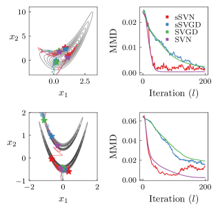
Figure 1: Two-dimensional experiments. Top row is a Hybrid-Rosenbrock density with parameters $n_{2}=1$, $n_{1}=2$, $a=0.5$, $b=0.5$, and the bottom row is a double-banana. The left column illustrates the geometry of the posterior, and displays the trajectory one of the particles follows along the various dynamics. The right column displays the evolution of the MMD using $N=100$ particles and 300 samples from the ground truth.

We begin with two low dimensional toy problems. The first is the Hybrid Rosenbrock distribution Pagani et al., (2020) with parameters $n_{2}=1$, $n_{1}=2$, $a=0.5$, and $b=0.5$, and the second is a double banana as described in Detommaso et al., (2018). We use $N=100$ particles, initially sampled from $\operatorname{Unif}[-6,6]$, and evolve for $L=200$ iterations with step size $\tau=0.1$.

Fig. 1 illustrates particle trajectories traced out by SVGD, SVN, and their stochastic counterparts. Of particular interest is that sSVN appears more efficient in its exploration of the posterior—in the sense that it explores more of the posterior in the same amount of time. In addition, the sSVN noise appears to facilitate mode hopping. We observe that the deterministic and stochastic counterparts make similar progress in MMD.

The settings for the Hybrid Rosenbrock density and the step size in this numerical experiment were chosen deliberately in order to compare all flows at the same timescale. It is important to note we numerically observe that a posterior with sufficiently narrow ridges causes sSVGD to produce overflow errors if the stepsize is not sufficiently small (even for two-dimensional cases). On the contrary, sSVN inherits the desirable affine invariance of SVN, allowing for larger stepsizes that are more robust to narrow ridges. For the posteriors studied in this paper, we observe that $\tau=0.1$ is a good step size for sSVN, and $\tau=0.01$ for sSVGD. Our subsequent experiments use these values.

5.2 Five-dimensional test case

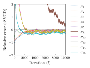
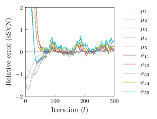
Figure 2: Five-dimensional experiments. Evolution of moments for sSVGD (top) and sSVN (bottom).

In this experiment we use a Hybrid Rosenbrock with parameters $n_{2}=2$, $n_{1}=3$, $a=10$, $b=30$ and compare only sSVGD and sSVN, using $N=100$ particles. We display the flow of the mean and variances of the ensemble to their converged values in Fig. 2. Interestingly, sSVGD requires over $10^{4}$ iterations for $\sigma_{11}$ to converge, wheras all moments converge rapidly within $100$ iterations in sSVN. We collect samples from the last $100$ iterations of both sSVGD and sSVN—neglecting issues related to sample autocorrelation for simplicity—and compare them to an i.i.d sample set of the same size in Fig. 3. The samples drawn from both sSVGD and sSVN appear to resemble the posterior well; however, sSVN exhibits an order of magnitude advantage in the number of iterations required. Since $N=100$, this corresponds to an $\mathcal{O}(10^{3})$ reduction in the number of gradient evaluations of the log-likelihood evaluations performed.

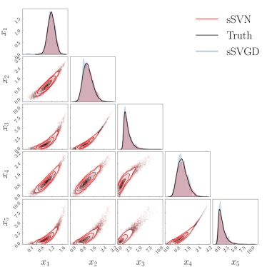
Figure 3: Five-dimensional Hybrid Rosenbrock corner plot comparing ground truth (black) with the output of sSVN (red) and sSVGD (blue). The diagonal figures compare one-dimensional KDEs of the marginals for sSVN, sSVGD, and ground truth. The off-diagonal figures compare only sSVN to ground truth for clarity, by plotting samples as well as contours in increments of $\sigma/2$ (sSVN) and a two-dimensional histogram of the density (ground truth).

5.3 Ten-dimensional test case

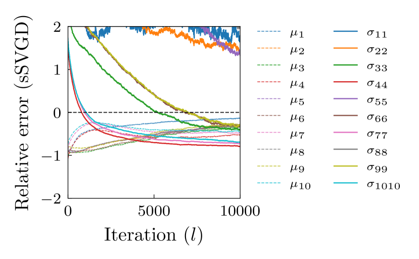
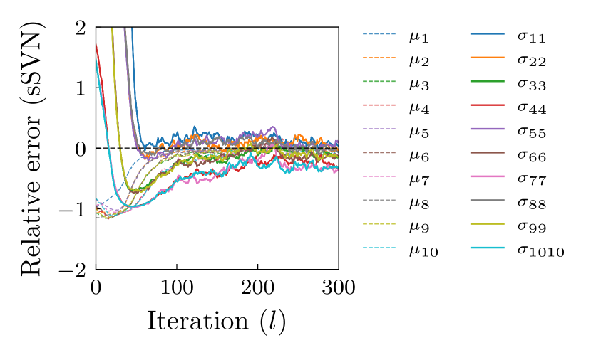
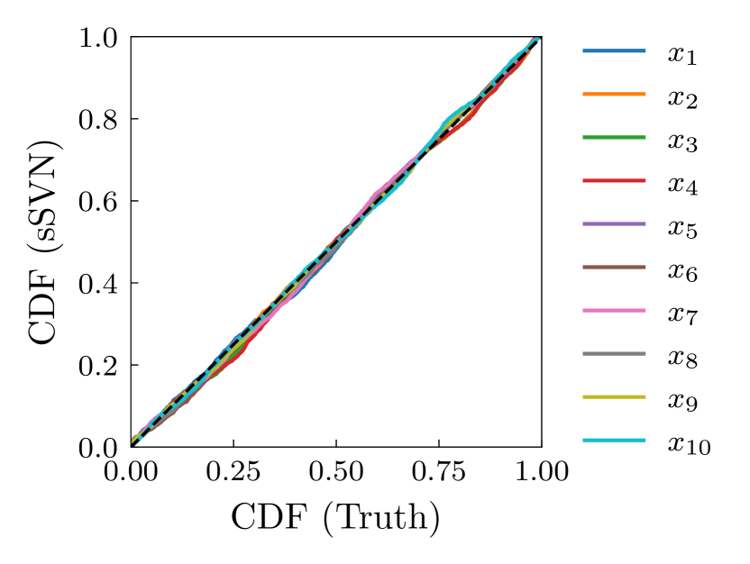
Figure 4: Results of ten-dimensional Hybrid Rosenbrock run. (Top) Evolution of means and variances under sSVGD dynamics. (Middle) Evolution of means and variances under sSVN dynamics. (Bottom) P-P plot of samples collected from iterations $200-300$ compared to two-million ground truth samples.

In this experiment we again use a Hybrid Rosenbrock, however with parameters $n_{2}=3$, $n_{1}=4$, $a=30$, $b=20$. We begin with $N=300$ particles drawn from $\operatorname{Unif}[-6,6]$, and run sSVGD and sSVN with $L=10000,300$ iterations respectively with an identity metric kernel. We plot the moment evolution in Fig. 4. Similar to the five dimensional case, it appears that sSVN equilibrates after $200$ iterations, while sSVGD struggles. As a measure of sample quality, we also present a P-P plot of the sSVN samples versus ground-truth, and find that they are in excellent agreement. To further investigate the convergence of sSVN, Fig. 5 collects samples from the final $100$ iterations and presents a corner plot comparing to $30000$ ground truth samples. We also compare the results of sSVN to sSVGD and ground truth in the one-dimensional marginals on the diagonal. The sSVN samples reconstruct the posterior accurately, as opposed to sSVGD, which has not yet converged.

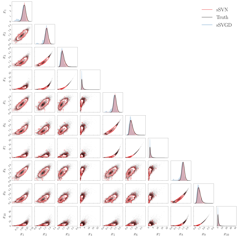
Figure 5: Same as Fig. 3, for the ten-dimensional Hybrid Rosenbrock density.

.

6 Discussion and further work

In contrast to its deterministic counterpart (SVN), sSVN may be made asymptotically correct by incorporating either a damping schedule or a Metropolis-Hastings correction, leading to a promising new approach to solving Bayesian inference tasks that require high-precision posterior reconstruction. To demonstrate the performance of our proposed algorithm, we examined the flows and sample quality on a difficult class of test problems—the Hybrid Rosenbrock density—and showed that sSVN successfully reconstructs the posterior with at least three orders of magnitude fewer gradient evaluations of the log-likelihood than sSVGD. In future work, it will be interesting to compare sSVN to other state of the art sampling algorithms such as dynamic nested sampling Higson et al., (2019); Skilling, (2006) and Hamiltonian Monte Carlo Betancourt, (2018); Neal et al., (2011). Further improvements to the algorithm are possible as well. For example, a Metropolis-Hastings correction may be implemented to eliminate all bias in the underlying Markov chain, random Fourier-feature kernels Liu and Wang, (2018) may be used to improve the descent direction, and gradient evaluations of the log-likelihood may be used to mitigate issues related to auto-correlation Riabiz et al., (2022); Hawkins et al., (2022).

Acknowledgements We thank Bassel Saleh and Peng Chen for discussions of Stein Variational methods at the outset of this work. A.Z. is supported by NSF Grant Number PHY-1912578.

Appendix A SVN simulates WNF

Recall from Wang and Li, (2020) that the WNF direction is a conservative vector field $w$ satisfying the following equation

$$\nabla_{i}\nabla_{j}\brk[r]{\rho\nabla_{i}w_{j}}-\nabla_{i}\brk[r]{\rho w_{j}\nabla_{i}\nabla_{j}f}-\nabla_{i}\brk[r]{\rho\nabla_{i}f}-\Delta\rho=0\>,$$ (20)

and that the Wasserstein gradient flow direction is a conservative velocity field defined by $v^{\text{GF}}\coloneqq-\nabla f-\nabla\ln\rho$, where the potential $f$ is a scalar field. Note that we are using Einstein summation convention, where repeated indices are summed over. Therefore

$$\nabla_{i}\brk[r]{\rho v^{\text{GF}}_{i}}=-\nabla_{i}\brk[s]!{\rho\brk[r]{\nabla_{i}f+\nabla_{i}\ln\rho}}=-\nabla_{i}(\rho\nabla_{i}f)-\Delta\rho\>,$$

where $\Delta$ denotes the Laplacian. Plugging this back into Eq. 20 yields

$$0 =\nabla_{i}\nabla_{j}(\rho\nabla_{i}w_{j})-\nabla_{i}(\rho w_{j}\nabla_{i}\nabla_{j}f)+\nabla_{i}(\rho v^{\text{GF}}_{i})$$

$$=\nabla_{i}\brk[s]!{\rho\nabla_{j}\ln\rho\nabla_{i}w_{j}+\rho\nabla_{i}\nabla_{j}w_{j}-\rho w_{j}\nabla_{i}\nabla_{j}f+\rho v^{\text{GF}}_{i}}$$

$$=\nabla_{j}\ln\rho\nabla_{i}w_{j}+\nabla_{i}\nabla_{j}w_{j}-w_{j}\nabla_{i}\nabla_{j}f+v^{\text{GF}}_{i}+\frac{\xi_{i}}{\rho}$$

$$=-(\tilde{H}w)_{i}+v^{\text{GF}}_{i}+\frac{\xi_{i}}{\rho}\>,$$ (21)

where $\xi$ is a divergence-free vector field, and we have defined

$$(\tilde{H}w)_{i}=-\nabla_{j}\ln\rho\nabla_{i}w_{j}-\nabla_{i}\nabla_{j}w_{j}+w_{j}\nabla_{i}\nabla_{i}f.$$ (22)

Eq. 21 illustrates how the Newton flow $w$ is related to the gradient flow $v^{\text{GF}}$.

We will now show that the weak form of Eq. 21 is releated to the variational characterization of the SVN direction given in Theorem 1 of Detommaso et al., (2018). Suppose $v$ is a conservative vector field restricted to the vector-valued reproducing kernel Hilbert space (RKHS) defined by $\mathcal{H}^{d}\coloneqq\mathcal{H}\times\mathcal{H}\times\cdots\times\mathcal{H}$, where $\mathcal{H}$ is an RKHS with kernel $k$. Let $T$ denote the embedding operator, which is defined by $(Tv)(y)=\int\rho(x)v(x)k(x,y)\>dx$, and let $\mathcal{L}_{\rho}^{2}$ denote the space of vector fields with finite squared norm with respect to $\rho$. Then by the embedding property Steinwart and Christmann, (2008) we have

$$\brk[a]1{\tilde{H}w-v^{\text{GF}},v}_{\mathcal{L}_{\rho}^{2}}=\brk[a]1{T(\tilde{H}w)-Tv^{\text{GF}},v}_{\mathcal{H}^{d}}=\int\xi\cdot v\>dx=0\>,$$ (23)

where the last equality holds since $\xi$ and $v$ are orthogonal. It has been shown in Theorem 2 of Liu et al., 2019a that $\brk[a]1{v^{\text{GF}},v}_{\mathcal{L}_{\rho}^{2}}=\brk[a]1{v^{\text{SVGD}},v}_{\mathcal{H}^{d}}$. Building on this, we have

$$\brk[s]!{T(\tilde{H}w)}_{i}(y) =\int\rho(x)\brk[s]!{-\nabla_{j}\ln\rho(x)\nabla_{i}w_{j}(x)-\nabla_{i}\nabla_{j}w_{j}(x)+w_{j}(x)\nabla_{i}\nabla_{j}f(x)}k(x,y)\>dx$$

$$=\int\brk[s]!{-\nabla_{j}\rho(x)\nabla_{i}w_{j}(x)k(x,y)-\rho(x)\nabla_{i}\nabla_{j}w_{j}(x)k(x,y)+\rho(x)\brk[a]1{w_{j}(\cdot),k(x,\cdot)}_{\mathcal{H}}\nabla_{i}\nabla_{j}f(x)k(x,y)}\>dx$$

$$=\int\rho(x)\nabla_{i}w_{j}(x)(\nabla_{1})_{j}k(x,y)\>dx+\brk[a]1{w_{j}(\cdot),\int\rho(x)\nabla_{i}\nabla_{j}f(x)k(x,\cdot)k(x,y)\>dx}_{\mathcal{H}}$$

$$=\brk[a]1{w_{j}(\cdot),\operatorname*{\mathbb{E}}_{x\sim\rho}\brk[s]!{(\nabla_{1})_{i}k(x,\cdot)(\nabla_{1})_{j}k(x,y)+\nabla_{i}\nabla_{j}f(x)k(x,\cdot)k(x,y)}}_{\mathcal{H}}=\brk[a]!{w_{j}(\cdot),h_{ij}(\cdot,y)}_{\mathcal{H}},$$ (24)

where the last equality defines $h(\cdot,y)$, which is equivalent to the SVN Hessian of Eq. 11 when evaluated at two particles $z_{m}$ and $z_{n}$, and when identifying $f=-\ln\pi$. The results Appendix A and Eq. 23, together with this definition of $f$, reproduce the characterization of the SVN direction in Detommaso et al., (2018). Thus, we may understand SVN as an RKHS approximation to WNF which does not enforce that the velocity field be conservative.

Remark A.1.

This result allows us to understand sSVN as an MCMC algorithm that uses as its proposal an approximated Wasserstein Newton step, plus a random forcing term which depends on the Hessian. In this way, sSVN is very similar to stochastic Newton (SN) discussed in Martin et al., (2012) and Section 2. However, a key distinction is that sSVN yields an interacting particle system and performs its optimization on the space of probability measures, as opposed to parameter space.

Appendix B Proofs

$$\left[\begin{array}[]{ccc}x_{1}\\ y_{1}\\ \hline\cr x_{2}\\ y_{2}\\ \hline\cr x_{3}\\ y_{3}\end{array}\right]$$

(a)

$$\left[\begin{array}[]{ccc}x_{1}\\ x_{2}\\ x_{3}\\ \hline\cr y_{1}\\ y_{2}\\ y_{3}\end{array}\right]$$

(b)

Figure 6: The index functions $\phi(m,i)$ and $\gamma(i,m)$ return the index of the $i^{\text{th}}$ coordinate of particle $m$ in the particle and dimension ordering respectively. For example, if $N=3,d=2$, then the vector $z$ in the particle ordering (a) has $z_{\phi(2,1)}=x_{2}$, while in the dimension ordering (b) has $z_{\gamma{(1,2)}}=y_{1}$.

Please refer to Fig. 6 for the definitions of the index maps $\phi$ and $\gamma$.

B.1 Proof of Lemma 3.1

Proof.

We begin by taking Eq. 6 and expressing it in index notation

$$\diff{z_{\phi(m,i)}}{t}=\sum_{j,n}\brk[s]1{K_{\phi(m,i)\phi(n,j)}\nabla_{\phi(n,j)}\ln\pi+\nabla_{\phi(n,j)}K_{\phi(m,i)\phi(n,j)}}\,,$$ (25)

where repeated indices are summed. The application of $K$ on any vector, and in particular $\nabla\ln\pi$, is to kernel average each particle block. In order to see this we proceed in index notation

$$\sum_{j,n}K_{\phi(m,i)\phi(n,j)}\nabla_{\phi(n,j)}\ln\pi =\frac{1}{N}\sum_{j,n}\brk[s]1{\bar{k}_{mn}\delta_{ij}\nabla_{j}\ln\pi(z_{n})}=\frac{1}{N}\sum_{n}\bar{k}_{mn}\nabla_{i}\ln\pi(z_{n})\,.$$ (26)

This shows the equivalence of the first terms on the right hand side of Eq. 2 and Eq. 6, which is the driving force of SVGD. Likewise, we have

$$\sum_{j,n}\nabla_{\phi(n,j)}K_{\phi(m,i)\phi(n,j)} =\frac{1}{N}\sum_{j,n}\brk[c]2{\delta_{ij}\brk[s]1{(\nabla_{1})_{j}\,\bar{k}_{mn}\delta_{mn}+(\nabla_{2})_{j}\,\bar{k}_{mn}}}=\frac{1}{N}(\nabla_{1})_{i}\bar{k}_{mm}+\frac{1}{N}\sum_{n}(\nabla_{2})_{i}\bar{k}_{mn}\,,$$ (27)

which shows the equivalence of the second terms on the right hand side of of Eq. 2 and Eq. 6 when the kernel has a “flat top”. In other words, for any $1\leq m\leq N$, $\nabla_{1}k(z_{m},z_{m})=0$. Finally, we show that $K$ inherits its positive (semi) definiteness from the kernel gram matrix $\bar{k}$. Since $K_{\phi(m,i)\phi(n,j)}\coloneqq\bar{k}_{mn}\delta_{ij}$ remains the same upon exchanging $m,n$ and $i,j$, $K$ is symmetric. Finally, recall that $K$ is orthogonal to $D_{K}$, and therefore both matrices have identical eigenvalues. Furthermore, since $D_{K}$ is block diagonal, its eigenvalues are equivalent to the eigenvalues of $\bar{k}$, repeated $N$ times. Therefore $K$ inherits its definiteness from $\bar{k}$. ∎

B.2 Proof that $PKP^{\top}=D_{K}$

Clearly it is important to recognize that $PKP^{\top}=D_{K}$ in order for sSVGD to be tractable: instead of calculating the Cholesky decomposition of an $Nd\times Nd$ matrix, this result suggests that only a $N\times N$ decomposition is necessary. This may be seen as a consequence of the following result.

Lemma B.1 (Basis transformation).

Let $P$ be the permutation matrix which takes a vector $v\in\mathbb{R}^{Nd}$ in the particle representation to the dimension representation. Then $M^{\prime}=PMP^{\top}$, where

$$M =\left[\begin{array}[]{ccc|c|ccc}M_{11}^{11}&\cdots&M^{11}_{1D}&&M^{1N}_{11}&\cdots&M^{1N}_{1D}\\ \vdots&\ddots&\vdots&\ldots&\vdots&\ddots&\vdots\\ M^{11}_{D1}&\cdots&M^{11}_{DD}&&M^{1N}_{DD}&\cdots&M^{1N}_{DD}\\ \hline\cr&\vdots&&\ddots&&\vdots\\ \hline\cr\rule{0.0pt}{14.22636pt}M^{N1}_{11}&\cdots&M^{N1}_{1D}&&M^{NN}_{11}&\cdots&M^{NN}_{1D}\\ \vdots&\ddots&\vdots&\ldots&\vdots&\ddots&\vdots\\ M^{N1}_{D1}&\cdots&M^{N1}_{DD}&&M^{NN}_{D1}&\cdots&M^{NN}_{DD}\end{array}\right] M^{\prime} =\left[\begin{array}[]{ccc|c|ccc}M_{11}^{11}&\cdots&M^{1N}_{11}&&M^{11}_{1D}&\cdots&M^{1N}_{1D}\\ \vdots&\ddots&\vdots&\ldots&\vdots&\ddots&\vdots\\ M^{N1}_{11}&\cdots&M^{NN}_{11}&&M^{N1}_{1D}&\cdots&M^{NN}_{1D}\\ \hline\cr&\vdots&&\ddots&&\vdots\\ \hline\cr\rule{0.0pt}{14.22636pt}M^{11}_{D1}&\cdots&M^{1N}_{D1}&&M^{11}_{DD}&\cdots&M^{1N}_{DD}\\ \vdots&\ddots&\vdots&\ldots&\vdots&\ddots&\vdots\\ M^{N1}_{D1}&\cdots&M^{1N}_{D1}&&M^{N1}_{DD}&\cdots&M^{NN}_{DD}\end{array}\right]$$

and $M^{mn}_{ij}\coloneqq M_{\phi(m,i)\phi(n,j)}$.

Proof.

Note that $PMP^{\top}=\brk[r]1{P(PM)^{\top}}^{\top}$. Beginning with $M$ we have

$$\xrightarrow{\textrm{Apply}P}\left[\begin{array}[]{ccc|c|ccc}M_{11}^{11}&\cdots&M^{11}_{1D}&&M^{1N}_{11}&\cdots&M^{1N}_{1D}\\ \vdots&\ddots&\vdots&\ldots&\vdots&\ddots&\vdots\\ M^{N1}_{11}&\cdots&M^{N1}_{1D}&&M^{NN}_{11}&\cdots&M^{NN}_{1D}\\ \hline\cr&\vdots&&\ddots&&\vdots\\ \hline\cr\rule{0.0pt}{14.22636pt}M^{11}_{D1}&\cdots&M^{11}_{DD}&&M^{1N}_{D1}&\cdots&M^{1N}_{DD}\\ \vdots&\ddots&\vdots&\ldots&\vdots&\ddots&\vdots\\ M^{N1}_{D1}&\cdots&M^{N1}_{DD}&&M^{NN}_{D1}&\cdots&M^{NN}_{DD}\end{array}\right]\xrightarrow{\textrm{Transpose}}\left[\begin{array}[]{ccc|c|ccc}M_{11}^{11}&\cdots&M^{N1}_{11}&&M^{11}_{D1}&\cdots&M^{N1}_{D1}\\ \vdots&\ddots&\vdots&\ldots&\vdots&\ddots&\vdots\\ M^{11}_{1D}&\cdots&M^{N1}_{1D}&&M^{11}_{DD}&\cdots&M^{N1}_{DD}\\ \hline\cr&\vdots&&\ddots&&\vdots\\ \hline\cr\rule{0.0pt}{14.22636pt}M^{1N}_{11}&\cdots&M^{NN}_{11}&&M^{1N}_{D1}&\cdots&M^{NN}_{D1}\\ \vdots&\ddots&\vdots&\ldots&\vdots&\ddots&\vdots\\ M^{1N}_{1D}&\cdots&M^{NN}_{1D}&&M^{1N}_{DD}&\cdots&M^{NN}_{DD}\end{array}\right]$$

$$\xrightarrow{\textrm{Apply}P}\left[\begin{array}[]{ccc|c|ccc}M_{11}^{11}&\cdots&M^{N1}_{11}&&M^{11}_{D1}&\cdots&M^{N1}_{D1}\\ \vdots&\ddots&\vdots&\ldots&\vdots&\ddots&\vdots\\ M^{1N}_{11}&\cdots&M^{NN}_{11}&&M^{1N}_{D1}&\cdots&M^{NN}_{D1}\\ \hline\cr&\vdots&&\ddots&&\vdots\\ \hline\cr\rule{0.0pt}{14.22636pt}M^{11}_{1D}&\cdots&M^{11}_{DD}&&M^{11}_{DD}&\cdots&M^{N1}_{DD}\\ \vdots&\ddots&\vdots&\ldots&\vdots&\ddots&\vdots\\ M^{1N}_{1D}&\cdots&M^{NN}_{1D}&&M^{1N}_{DD}&\cdots&M^{NN}_{DD}\end{array}\right]\xrightarrow{\textrm{Transpose}}\left[\begin{array}[]{ccc|c|ccc}M_{11}^{11}&\cdots&M^{1N}_{11}&&M^{11}_{1D}&\cdots&M^{1N}_{1D}\\ \vdots&\ddots&\vdots&\ldots&\vdots&\ddots&\vdots\\ M^{N1}_{11}&\cdots&M^{NN}_{11}&&M^{N1}_{1D}&\cdots&M^{NN}_{1D}\\ \hline\cr&\vdots&&\ddots&&\vdots\\ \hline\cr\rule{0.0pt}{14.22636pt}M^{11}_{D1}&\cdots&M^{1N}_{D1}&&M^{11}_{DD}&\cdots&M^{1N}_{DD}\\ \vdots&\ddots&\vdots&\ldots&\vdots&\ddots&\vdots\\ M^{N1}_{D1}&\cdots&M^{1N}_{D1}&&M^{N1}_{DD}&\cdots&M^{NN}_{DD}\end{array}\right]$$

∎

The result follows from observing that the $\delta_{ij}$ term in $K$ kills off all off diagonal blocks.

B.3 Proof of Theorem 4.1

Proof.

We show that Eq. 14 may be derived from Eq. 3 with diffusion matrix $D^{\text{SVN}}\coloneqq NKH^{-1}K$, and curl matrix $Q=0$. Direct substitution yields

$$\>dz =\brk[r]{D^{\text{SVN}}\nabla\ln\pi+\nabla\cdot D^{\text{SVN}}}\>dt+\sqrt{2D^{\text{SVN}}}\>dB$$

$$=\brk[s]1{(NKH^{-1}K)\nabla\ln\pi+\nabla\cdot\brk[r]{NKH^{-1}K}}\>dt+\sqrt{2D^{\text{SVN}}}\>dB\,.$$

We focus only on the drift term and proceed in index notation, expanding the divergence and collecting terms

$$NK_{ab}H^{-1}_{bc}K_{ce}\nabla_{e}\ln\pi+N\nabla_{e}(K_{ab}H^{-1}_{bc}K_{ce}) =\overbrace{NK_{ab}H^{-1}_{bc}(K_{ce}\nabla_{e}\ln\pi+\nabla_{e}K_{ce})}^{v^{\text{SVN}}}+\overbrace{\nabla_{e}(K_{ab}H^{-1}_{bc})K_{ce}}^{v^{\textrm{DET}}}\,,$$ (28)

which gives the stated form of $v^{\textrm{DET}}$. Finally, since $K$ is invertible, $KH^{-1}K$ is a congruence transformation of $H^{-1}$, and thus if $H^{-1}$ is positive definite, so is $D^{\text{SVN}}$. ∎

Remark B.2.

The assumption that $H$ be strictly positive definite is necessary to ensure that $v^{\text{SVN}}$ leads to a valid search direction. Indeed, this is not true in general, and requires careful consideration. See the discussion preceding Theorem 4.1 and Levenberg damping for a discussion on how to ensure $H$ is positive definite.

Remark B.3.

We may express $v^{\textrm{DET}}$ in the form

$$v^{\textrm{DET}}_{a} =N[(\nabla_{e}(K_{ab})H^{-1}_{bc}K_{ce}-K_{ab}H^{-1}_{bf}(\nabla_{e}H_{fg})H^{-1}_{gc}K_{ce}]$$

using the identity $\nabla_{e}H^{-1}_{bc}=-H_{bf}^{-1}(\nabla_{e}H_{fg})H^{-1}_{fc}$. This expression illustrates that third derivatives are required to compute $v^{\textrm{DET}}$ in general, and second derivatives are required even with the Gauss Newton approximation. Note that similar terms appear in other higher-order flows, and are often neglected. See the paragraph on asymptotic correctness in Section 4.2 for further discussion.

Appendix C Scaling improvements

In Algorithm 3 we form the SVN Hessian $H$, find the Cholesky decomposition of $H$, and use the decomposition to find the descent direction and calculate the noise. However, for large $N,d$, the Cholesky decomposition and the associated storage requirements may be costly. In this section we propose an alternative scheme utilizing conjugate gradients—whose iterations may be terminated when desired, and only requires the ability to evaluate matrix-vector products, thus circumventing the need to form $H$.

Observe that

$$z^{l+1} =z^{l}+\tau NKH^{-1}v^{\text{SVGD}}+\sqrt{\tau}\mathcal{N}(0,2NKH^{-1}K)$$

$$=z^{l}+\tau NKH^{-1}v^{\text{SVGD}}+\sqrt{2N\tau}KH^{-1}H\mathcal{N}(0,H^{-1})$$

$$=z^{l}+\tau NKH^{-1}\brk[s]!{v^{\text{SVGD}}+\sqrt{\frac{2}{N\tau}}\mathcal{N}(0,H)}$$ (29)

We now show that $\mathcal{N}(0,H)$ may be sampled efficiently. To begin, note that the SVN Hessian may be re-expressed as

$$H=H^{(1)}+H^{(2)}=NKH_{\pi}K+H^{(2)}\,,$$ (30)

where $H_{\pi},H^{(2)}\in\mathbb{R}^{Nd\times Nd}$ are both block diagonal matrices whose $m^{\rm th}$ $d\times d$ blocks are given by $\nabla^{2}\ln\pi(z_{m})$, and $\frac{1}{N}\sum_{n}\nabla_{1}k(z_{m},z_{n})\nabla_{1}^{\top}k(z_{m},z_{n})$ respectively. Indeed, we can see by

$$NKH_{\pi}K =NK_{\phi(m,i)\phi(l,e)}(H_{\pi})_{\phi(l,e)\phi(p,f)}K_{\phi(p,f)\phi(n,j)}$$

$$=\frac{1}{N}\sum_{e,f}\sum_{l,p}\brk[s]1{\delta_{lp}\bar{k}_{ml}\bar{k}_{pn}\delta_{ie}\delta_{fj}\nabla_{e}\nabla_{f}\ln\pi(z_{l})}$$

$$=\frac{1}{N}\sum_{l}\brk[s]1{\bar{k}_{ml}\bar{k}_{ln}\nabla_{i}\nabla_{j}\ln\pi(z_{l})}\,,$$

that $H^{(1)}$ corresponds to the first term in Eq. 11. The noise term may thus be decomposed as

$$\mathcal{N}(0,H)=\mathcal{N}(0,NKH_{\pi}K+H^{(2)})=\sqrt{N}K\mathcal{N}(0,H_{\pi})+\mathcal{N}(0,H^{(2)})\,.$$ (31)

Now, since $H_{\pi}$ is block diagonal, the task of drawing the first term in Eq. 31 decomposes into $N$ individual $d\times d$ subproblems, which may be solved with $N\times(d\times d)$ Cholesky decompositions. The second term simplifies as well. The $m^{\rm th}$ block of $\mathcal{N}(0,H^{(2)})$ may be evaluated with

$$\mathcal{N}\brk[r]2{0,\frac{1}{N}\sum_{n}\nabla_{1}k(z_{m},z_{n})\nabla_{1}^{\top}k(z_{m},z_{n})} =\frac{1}{\sqrt{N}}\sum_{n}\mathcal{N}\brk[r]2{0,\nabla_{1}k(z_{m},z_{n})\nabla_{1}^{\top}k(z_{m},z_{n})}$$

$$=\frac{1}{\sqrt{N}}\sum_{n}\nabla_{1}k(z_{m},z_{n})\mathcal{N}_{mn}\,,$$ (32)

where for every $1\leq m,n\leq N$, $\mathcal{N}_{mn}$ denotes a sample from a standard normal. Thus, a draw from $\mathcal{N}(0,H)$ has a cost of $\mathcal{O}(Nd^{3})$, as opposed to $\mathcal{N}(0,H^{-1})$, which has a (time complexity) cost of $\mathcal{O}(N^{3}d^{3})$. Meanwhile, with the use of a CG solver, we no longer need to form the SVN Hessian, thus improving memory complexity by a factor of $N$.

This scheme is thus a simple modification of the original “full SVN” algorithm. Namely, the only change is we instead work with a noise perturbed SVGD direction $v^{\text{SVGD}}_{*}=v^{\text{SVGD}}+\sqrt{2/(N\tau)}\mathcal{N}(0,H)$. A summary is provided in Algorithm 4.

Input: Initialize ensemble $z^{1}$, $\tau>0$

for $l=1,2,\ldots,L$ do

       Calculate perturbed SVGD direction $v^{\text{SVGD}}_{*}$ Eq. 29 ;

       Define method yielding Hessian-vector product $Hv$, $v\in\mathbb{R}^{Nd}$ ;

       CG solve: $Hv^{\text{SVN}}_{*}=v^{\text{SVGD}}_{*}$ ;

       $z^{l+1}\leftarrow z^{l}+\tau v^{\text{SVN}}_{*}(z^{l})$ ;

      

end for

Algorithm 4 Stochastic SVN (CG)

Remark on block diagonal SVN

The block diagonal approximation, originally introduced in Detommaso et al., (2018), considers only the diagonal blocks $h^{mm}$ where $1\leq m\leq N$ of the Hessian $H$. In turn, this decouples the solves necessary to perform Eq. 9 from an $Nd\times Nd$ to $N\times(d\times d)$ solves. Finally, the approximation takes $\alpha$ to be the step direction directly, as opposed to using Eq. 12. This significantly reduces the burden of solving the linear system and improves scalability. Unfortunately, this scheme does not naturally extend to the stochastic case. Specifically, notice that if one were to design a stochastic block diagonal algorithm, the leading term would be $H^{-1}K\nabla\ln\pi$. The primary issue with $H^{-1}K$ is that it is dense, and not symmetric. The cost of the Cholesky decomposition remains $\mathcal{O}(N^{3}d^{3})$, at which point the full Hessian may as well be used.

References

• Abbott et al., (2021) Abbott, R. et al. (2021). GWTC-3: Compact Binary Coalescences Observed by LIGO and Virgo During the Second Part of the Third Observing Run.
• Aghanim et al., (2020) Aghanim, N. et al. (2020). Planck 2018 results. VI. Cosmological parameters. Astron. Astrophys., 641:A6. [Erratum: Astron.Astrophys. 652, C4 (2021)].
• Anonymous, (2022) Anonymous (2022). Understanding the Variance Collapse of SVGD in High Dimensions. In Submitted to The Tenth International Conference on Learning Representations. under review.
• Betancourt, (2018) Betancourt, M. (2018). A Conceptual Introduction to Hamiltonian Monte Carlo.
• Blei et al., (2017) Blei, D. M., Kucukelbir, A., and McAuliffe, J. D. (2017). Variational Inference: A Review for Statisticians. Journal of the American Statistical Association, 112(518):859–877.
• Chen and Ghattas, (2020) Chen, P. and Ghattas, O. (2020). Projected Stein Variational Gradient Descent.
• Chen et al., (2020) Chen, P., Wu, K., Chen, J., O’Leary-Roseberry, T., and Ghattas, O. (2020). Projected Stein variational Newton: A fast and scalable Bayesian inference method in high dimensions.
• D’Angelo and Fortuin, (2021) D’Angelo, F. and Fortuin, V. (2021). Annealed Stein Variational Gradient Descent.
• Detommaso et al., (2018) Detommaso, G., Cui, T., Spantini, A., Marzouk, Y., and Scheichl, R. (2018). A Stein variational Newton method. Advances in Neural Information Processing Systems, 2018-Decem(Nips):9169–9179.
• Duncan et al., (2019) Duncan, A., Nüsken, N., and Szpruchz, L. (2019). On the Geometry of Stein Variational Gradient Descent.
• Gallego and Insua, (2020) Gallego, V. and Insua, D. R. (2020). Stochastic Gradient MCMC with Repulsive Forces. arXiv:1812.00071 [cs, stat].
• Gan et al., (1991) Gan, F. F., Koehler, K. J., and Thompson, J. C. (1991). Probability Plots and Distribution Curves for Assessing the Fit of Probability Models. The American Statistician, 45(1):14–21.
• Girolami and Calderhead, (2011) Girolami, M. and Calderhead, B. (2011). Riemann manifold Langevin and Hamiltonian Monte Carlo methods. Journal of the Royal Statistical Society: Series B (Statistical Methodology), 73(2):123–214.
• Gong et al., (2019) Gong, C., Peng, J., and Liu, Q. (2019). Quantile Stein Variational Gradient Descent for batch Bayesian optimization. In Chaudhuri, K. and Salakhutdinov, R., editors, Proceedings of the 36th International Conference on Machine Learning, volume 97 of Proceedings of Machine Learning Research, pages 2347–2356. PMLR.
• Gretton et al., (2012) Gretton, A., Borgwardt, K. M., Rasch, M. J., Schölkopf, B., and Smola, A. (2012). A Kernel Two-Sample Test. Journal of Machine Learning Research, 13(25):723–773.
• Gunapati et al., (2018) Gunapati, G., Jain, A., Srijith, P. K., and Desai, S. (2018). Variational inference as an alternative to MCMC for parameter estimation and model selection. arXiv: Instrumentation and Methods for Astrophysics.
• Hawkins et al., (2022) Hawkins, C., Koppel, A., and Zhang, Z. (2022). Online, Informative MCMC Thinning with Kernelized Stein Discrepancy.
• Higson et al., (2019) Higson, E., Handley, W., Hobson, M., and Lasenby, A. (2019). Dynamic Nested Sampling: An improved algorithm for parameter estimation and evidence calculation. Statistics and Computing.
• Jia et al., (2021) Jia, J., Li, P., and Meng, D. (2021). Stein variational gradient descent on infinite-dimensional space and applications to statistical inverse problems.
• Korba et al., (2021) Korba, A., Salim, A., Arbel, M., Luise, G., and Gretton, A. (2021). A Non-Asymptotic Analysis for Stein Variational Gradient Descent.
• Liu and Zhu, (2017) Liu, C. and Zhu, J. (2017). Riemannian Stein Variational Gradient Descent for Bayesian Inference.
• (22) Liu, C., Zhuo, J., Cheng, P., Zhang, R., Zhu, J., and Carin, L. (2019a). Understanding and accelerating particle-based variational inference. 36th International Conference on Machine Learning, ICML 2019, 2019-June:7187–7205.
• (23) Liu, C., Zhuo, J., and Zhu, J. (2019b). Understanding MCMC Dynamics as Flows on the Wasserstein Space. arXiv:1902.00282 [cs, stat].
• Liu, (2017) Liu, Q. (2017). Stein Variational Gradient Descent as Gradient Flow.
• Liu and Wang, (2016) Liu, Q. and Wang, D. (2016). Stein variational gradient descent: A general purpose Bayesian inference algorithm. In Advances in Neural Information Processing Systems.
• Liu and Wang, (2018) Liu, Q. and Wang, D. (2018). Stein Variational Gradient Descent as Moment Matching.
• Loy et al., (2015) Loy, A., Follett, L., and Hofmann, H. (2015). Variations of Q-Q Plots – The Power of our Eyes!
• Ma et al., (2015) Ma, Y.-A., Chen, T., and Fox, E. B. (2015). A Complete Recipe for Stochastic Gradient MCMC. arXiv:1506.04696 [math, stat].
• Martin et al., (2012) Martin, J., Wilcox, L. C., Burstedde, C., and Ghattas, O. (2012). A stochastic Newton MCMC method for large-scale statistical inverse problems with application to seismic inversion. SIAM Journal on Scientific Computing, 34(3):A1460–A1487.
• Neal et al., (2011) Neal, R. M. et al. (2011). MCMC using Hamiltonian dynamics. Handbook of markov chain monte carlo, 2(11):2.
• Pagani et al., (2020) Pagani, F., Wiegand, M., and Nadarajah, S. (2020). An n-dimensional Rosenbrock Distribution for MCMC Testing.
• Patterson and Teh, (2013) Patterson, S. and Teh, Y. W. (2013). Stochastic Gradient Riemannian Langevin Dynamics on the Probability Simplex. In Burges, C. J. C., Bottou, L., Welling, M., Ghahramani, Z., and Weinberger, K. Q., editors, Advances in Neural Information Processing Systems, volume 26. Curran Associates, Inc.
• Pinder et al., (2021) Pinder, T., Nemeth, C., and Leslie, D. (2021). Stein Variational Gaussian Processes.
• Qi and Minka, (2002) Qi, Y. and Minka, T. P. (2002). Hessian-based Markov chain Monte-Carlo algorithms.
• Riabiz et al., (2022) Riabiz, M., Chen, W., Cockayne, J., Swietach, P., Niederer, S. A., Mackey, L., and Oates, C. J. (2022). Optimal Thinning of MCMC Output.
• Skilling, (2006) Skilling, J. (2006). Nested sampling for general Bayesian computation. Bayesian Analysis.
• Speagle, (2020) Speagle, J. S. (2020). A conceptual introduction to Markov Chain Monte Carlo methods.
• Steinwart and Christmann, (2008) Steinwart, I. and Christmann, A. (2008). Support vector machines. Springer Science & Business Media.
• van de Schoot et al., (2021) van de Schoot, R., Depaoli, S., King, R., Kramer, B., Märtens, K., Tadesse, M. G., Vannucci, M., Gelman, A., Veen, D., Willemsen, J., et al. (2021). Bayesian statistics and modelling. Nature Reviews Methods Primers, 1(1):1–26.
• Wang and Li, (2020) Wang, Y. and Li, W. (2020). Information Newton’s flow: second-order optimization method in probability space.
• Zhang and Curtis, (2020) Zhang, X. and Curtis, A. (2020). Variational full-waveform inversion. Geophysical Journal International, 222(1):406–411.
• Zhang and Sutton, (2011) Zhang, Y. and Sutton, C. (2011). Quasi-Newton methods for Markov chain Monte Carlo. Advances in Neural Information Processing Systems, 24:2393–2401.
• Şimşekli et al., (2016) Şimşekli, U., Badeau, R., Cemgil, A. T., and Richard, G. (2016). Stochastic Quasi-Newton Langevin Monte Carlo.