Electric field-induced domain wall motion in spin spiral multiferroics
Abstract
Switching in magnetic materials gives rise to rich physical phenomena and lies at the heart of their technological applications. Although domain wall motion in ferro- and antiferromagnets has been studied Schryer and Walker (1974); Park et al. (2011); Duine (2011), in spiral magnets it is still poorly understood despite 20 years of active research since the discovery of spiral multiferroics Kimura et al. (2003); Cheong and Mostovoy (2007); Kimura et al. (2008); Mostovoy (2008); Rocquefelte et al. (2013). The problem of the domain wall motion in a spiral magnet is a compelling one, the more so the magnetic domain walls in cycloidal spiral phase are also ferroelectric, thus enabling electric control of magnetism, i.e. domain wall motion under the action of an external electric field. Phase transition to a spiral phase leads to a formation of chiral domains with opposite spin rotation senses, that are separated by chiral domain walls. Spiral order breaks inversion symmetry and induces a ferroelectric polarization, whose sign is determined by the chirality of the domain. Thus the spiral order allows for the manipulation of spins via an external electric field. Here we study domain wall motion in magnets with spiral ground state, that are the most basic non-collinear magnets. We formulate a simplified variational model and derive the equation of motion for the domain wall driven by an external electric field. The results are corroborated with atomistic spin dynamics simulations. The results suggest a linear dependence of the wall speed on the external electric field, and a peculiar dependence on the system geometry and domain structure.
Introduction — Magnetic frustration, or competition between various spin interactions, plays a fundamental role in magnetoelectric and multiferroic properties Diep (1994). Geometric frustration or competing nearest and next-nearest-neighbor exchange interactions can result in peculiar spin ordering, skyrmions and other non-collinear spin textures, and could lead to polar lattice distortions Cheong and Mostovoy (2007); Van Den Brink and Khomskii (2008); Leonov and Mostovoy (2015); Paul et al. (2020). This scenario is the ideal playground for complex spin textures and magnetoelectric coupling to appear Li et al. (2012); Cheong and Mostovoy (2007); Spaldin et al. (2008). In particular, the study of the DW and skyrmion dynamics has attracted experimental and theoretical interest in the recent years Kagawa et al. (2009); McQuaid et al. (2017); Brierley and Littlewood (2014); Whyte and Gregg (2015).
In this Letter we study domain wall motion in the most basic non-collinear magnet, one with a cycloidal spiral spin ordering, stabilized by competing exchange interactions, as in RMnO3, YMn2O5, MnWO4 or CuO Kimura et al. (2003); Cheong and Mostovoy (2007). Our aim is to investigate the motion of a DW, which we refer to as a chiral DW Li et al. (2019). In this context “chiral” refers to a system that is not identical to its mirror image and, in the particular case of the spiral spin order, a chiral domain is a region where the rotation sense of the spins is well-defined. Therefore, chirality is strictly related to the spin rotation sense, and a chiral DW is the region of separation between two domains of opposite chirality, i.e. opposite spin rotation senses.
While the concept of chirality in motion of chiral DWs have recently attracted attention Karna et al. (2021); Cohen et al. (2020); Qaiumzadeh et al. (2018); Schoenherr et al. (2018), to our knowledge, electric field driven switching in spiral magnets has not been studied. In a cycloidal spiral spin configuration, where the spin rotation plane contains the wave vector, inversion symmetry is broken, and a ferroelectric polarization emerges through inverse Dzyaloshinskii-Moriya (DM) effect Katsura et al. (2005); Mostovoy (2006); Sergienko and Dagotto (2006); Dong et al. (2019).
We proceed in the following way: we propose an Ansatz for the chiral DW profile and, using a variational approach, obtain the equations of motion for the DW. We study the cases of one single DW and two DWs moving in an external electric field in a quasi-1D geometry. The results of the model are then compared with the atomistic spin dynamics simulations. The last part of the Letter is dedicated to the discussion of the simulations. We observe that, even when starting with a single-DW configuration, another domain is nucleated at the boundary of the sample in the presence of the electric field. DWs do not behave as isolated objects and move according to the presence of other walls, as seen from the comparison of the one-DW and two-DW cases. The results suggest that the domains of polarization opposite to the external field shrink and finally disappear with the emission of magnons. The domain wall velocity in a linear response regime is proportional to the driving electric field and inversely proportional to the Gilbert damping and the distance to the boundary. No Walker breakdown is observed in simulations.
The Model – In order to study the motion of the chiral DWs, we consider a quasi-1D model, where a magnetization continuously varies along through an interval of total length . can be directed along all the three spatial directions.
The dynamics of the spiral magnet is described by the Lagrangian density Li et al. (2012); Auerbach (2012),
| (1) |
where is a constant that has the dimensions of an action, the first term describes the precession of the magnetization, with acting as a vector potential so that Auerbach (2012). and describe competing magnetic exchange constants, and produce spatial variation of the magnetization with the wavevector . is the electric field, that we will consider parallel to , and represents the coupling between the spiral order and the field, resulting from DM interaction and proportional to the spin-orbit coupling constant. is the hard axis anisotropy constant that forces spins into the -plane. As we will see from the following, the main contributions come from the domains, which suggests the dynamics to be largely independent of the DW type.
We also introduce the Rayleigh dissipation functional density
| (2) |
that describes the energy dissipation. is the damping constant and has dimensions of a momentum.
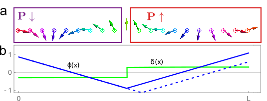
In order to describe a cycloidal spiral spin configuration with a single DW at the position , as seen in Fig. 1, we express the magnetization in spherical coordinates, , where the dependence on of the angles and is omitted for simplicity, and we assume the following Ansatz that captures the essential physics of the DW motion:
| (3) |
where is the wave vector of the spiral, i.e. the angle between two nearby spins; is the initial phase for the angle and (with ) represents the out-of-plane components of the spins. Here the shape of is inspired by the usual spiral solution in the model, however with a DW in the center.
The presence of the components of the magnetization encoded by is needed for the magnetization to rotate. Indeed, for the DW to move, spins must precess around axis. Magnetization precesses around the effective field that for spins lying in -plane has no component. The precession around axis becomes possible because the magnetization acquires component due to DM field, that has a component in plane perpendicular to the magnetization.
Results — In the spirit of a variational approach, we integrate and over the sample. We continue to refer to the integrated Lagrangian and Rayleigh functions with and for simplicity.
Using Euler-Lagrange equations we derive the equations of motions for the DW
| (4) |
where . We report in the Methods section of the Supplementary Information the detailed discussion of the model and the derivation of the following equations
| (5) | |||||
| (6) | |||||
| (7) | |||||
| (8) |
with . We note that are all linear in the field . As discussed in the Methods, here we neglected subleading terms. It is remarkable that the DW velocity is inversely proportional to the distance from the sample surfaces, and . Therefore, for a DW deep inside a large sample, , the speed goes to zero as , as demonstrated in recent experiments Biesenkamp2021; Stein2021. This can be understood from the fact that fewer spins have to be rotated in order to move the DW when it is near the boundary. It follows from Equations (5) and (6), that
| (9) |
a relation that also holds in the simulations. It is evident from Equations (5) and (7), that the rate of spin precession in the first domain in the steady state () is determined by . Analogously the rate in the second domain, , it is proportional to . Thus the torque on spins due to component is distributed according to the size of the domain, so that spins in the larger domain rotate less. This also explains why the DW velocity diverges when approaching the boundary.
The integration of Eq. (8) gives a cubic equation for . In the limit of , when the DW is near the sample boundary, the term dominates and we obtain
| (10) |
where we rewrote as for simplicity.
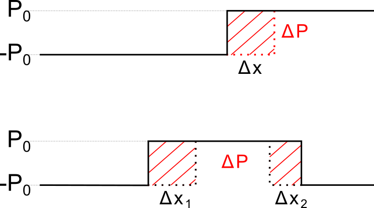
Two DWs — In real materials many DWs are present at the same time, so that when an electric field is applied on the whole sample, all the walls move. In a quasi-1D picture, we can think of the pairs of DWs delimiting domains of polarization opposite to the applied electric field. We expect for DWs in such pairs to move towards each other under the action of the field, so as to drive the compression of ferroelectric domains of unfavorable polarization. In analogy with the previous case, we use a modified Ansatz,
| (11) |
the notation is analogous to the single DW case, except for and that are the positions of the two DWs. We proceed as with the single-DW case and derive the equations of motion from and , truncating them to the lowest order in the external field . We obtain
| (12) |
We observe that, in the large- limit, the expressions for and become identical to those in the single DW case, Eq. (7), (8). It is interesting that the speeds of the two walls are opposite in sign but generally not equal in the absolute value. We can understand the dependence of the speed of the walls on their position by focusing on the spin texture.
By integrating the equations for the two walls we obtain
| (13) |
Simulations — In order to validate our model, we performed atomistic spin dynamics simulations using the UppASD code Skubic et al. (2008) (see Methods section for details).
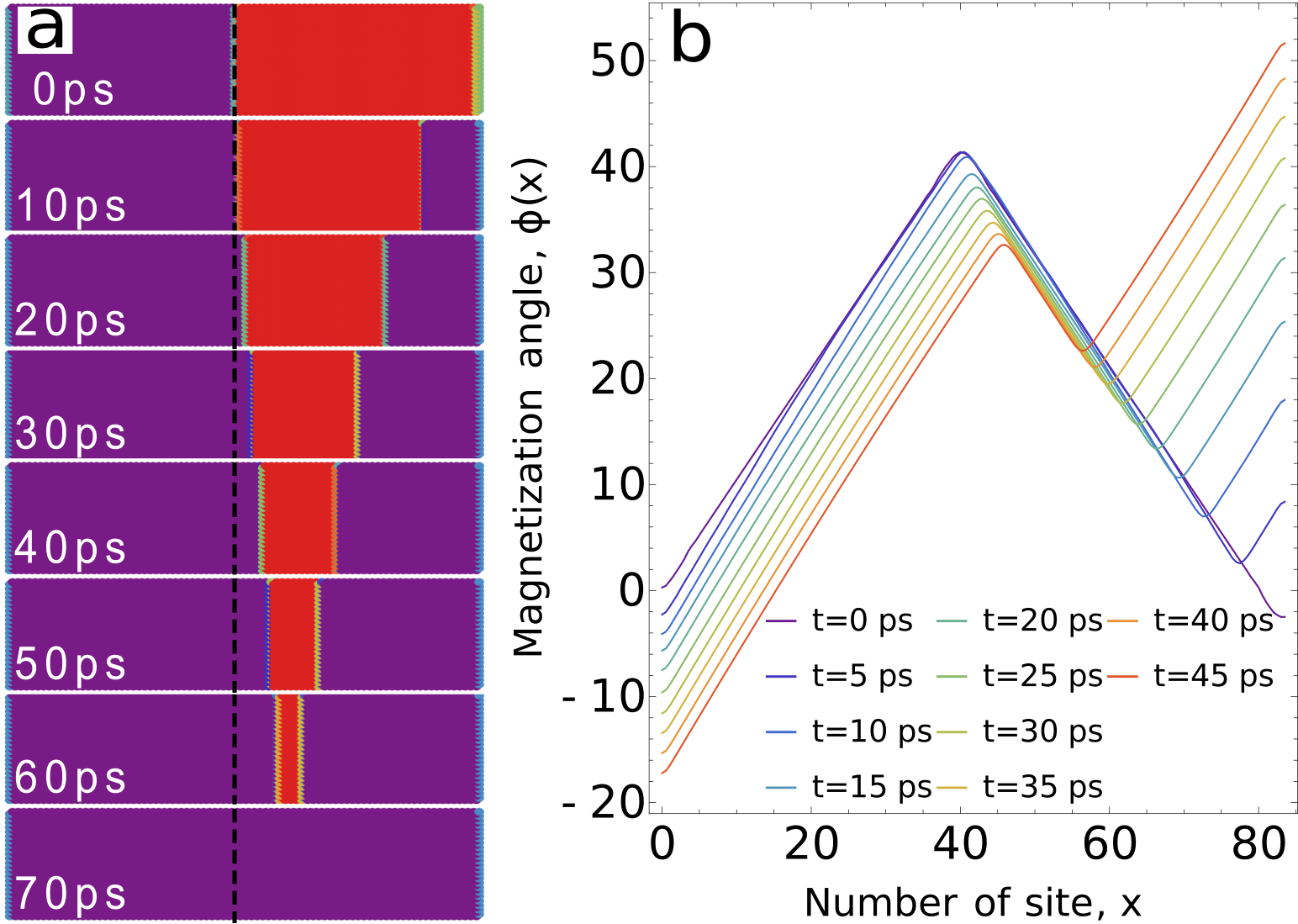
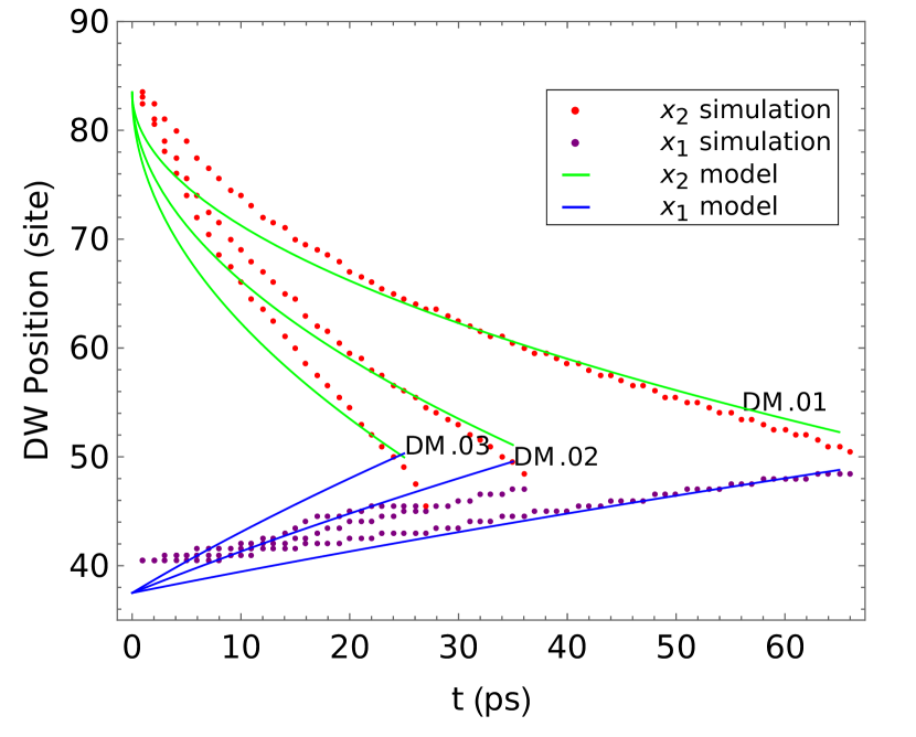
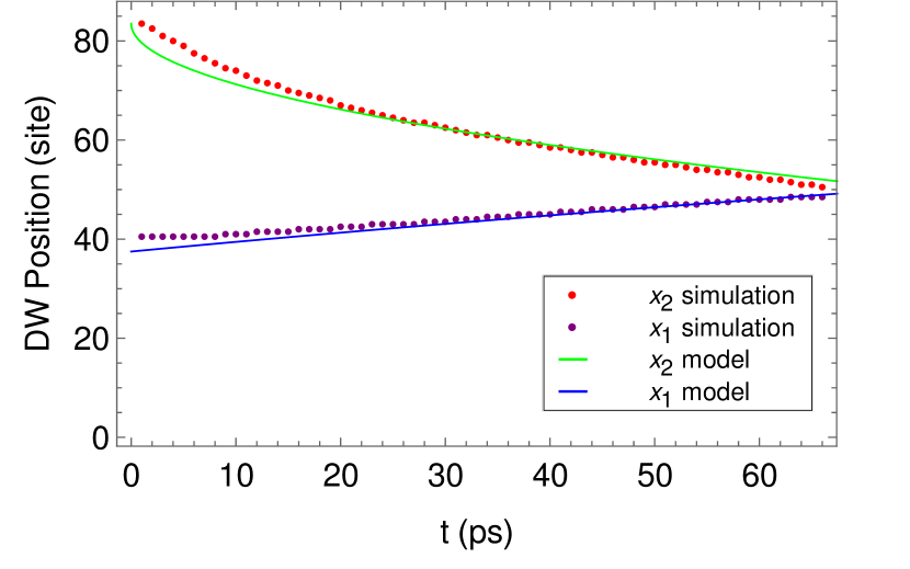
As we discussed before, in a quasi-1D picture and in the presence of an electric field, the energy of a domain is linear in its size, which could be seen as a linear potential between the walls. DWs associated with domains of the polarization opposite to the external field move in pairs. This is observed in our simulation where a new DW is formed at the right boundary. The DW at the center and at the boundary both move, however the wall in the center is slower, as seen in Fig. 2(a). This is due to the greater number of spins that have to be rotated by the torque arising due to the action of the field for the central wall to be moved. The two walls move towards each other, collide and annihilate at approximately 70 ps, leaving the system in a single domain state. Upon collision, magnons are excited and propagate away from the collision site, as seen in the Supplementary GIF. Magnons have oscillating signatures in the polarization profile, that propagate away from the collision site. The magnon emission may slightly alter the trajectory of the walls and thus generate a small difference with our model.
The rotation of the spins can be visualized by plotting , cf. Fig. 2. Straight lines represent uniform spin spiral and correspond to chiral domains, while V-shaped cusps are the DWs. Just after , a V-shape appears at the right boundary, indicating a nucleation of a second domain with P along the external field. The large distances between the right cusps at subsequent steps indicate large initial speed of the right DW, that is consistent with the discussion following Eq. (9) and the fact that the right domain is very narrow. As the nucleated domain on the right grows, the wall gets slower and the distances between the cusps decrease. The wall initially at the center starts with a lower velocity and just slightly accelerates while moving to the right.
We now compare the motion of the two walls with the predictions of Eq. (13). The simulated snapshots of the polarization texture at different times are shown in Fig. 2(a). Fig. 4 reports the DW trajectories from the simulations (dots) and the behaviour predicted by the model (solid lines).
We find good agreement between the simulation and the theory. Differences near may be due to a transient effect that is beyond our steady state solution. At large fields the differences between our linear-response theory and the simulations become more visible, as seen in the Supplementary Figure. S1.
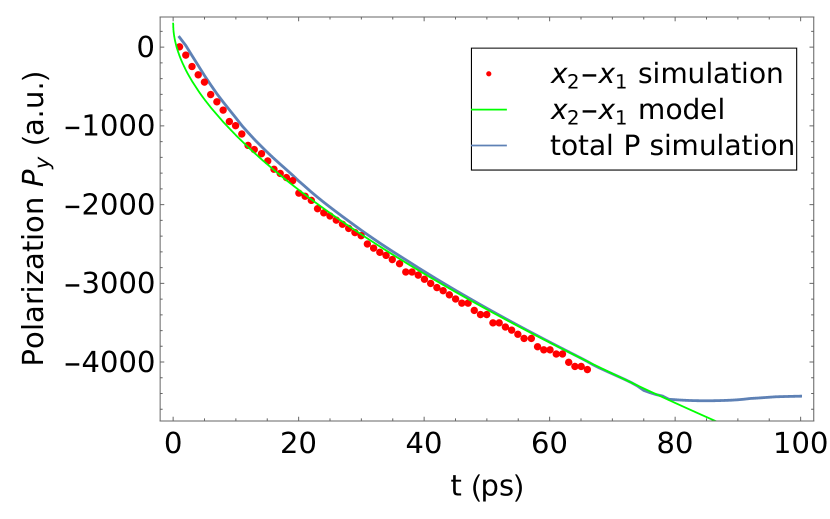
Supplementary Figure S2 shows the simulated time-dependent polarization that results from DW motion in Fig. 2. The initial polarization is zero as initially the two DWs with opposite chiralities and hence opposite polarizations have the same size. When the walls start moving, the domain with polarization along the field grows, and the polarization decreases towards negative values until it saturates when only one domain is left. Our model is also able to predict the polarization evolution, as seen in the Supplementary Figure S2. As the DWs move, the overall contribution to the polarization changes accordingly (see Fig. 3 for reference), and it is
| (14) |
Eq. (14) shows how the t-dependent polarization is related to the position of the walls. Polarization evolution obtained in simulations, Supplementary Figure. S2, matches well with Eq. (14).
Conclusions – In summary, we studied the dynamics of spiral multiferroics under an external electric field using a variational approach and numerical simulations. The equations of motion are derived. We find that the speed of the wall is proportional to the external electric field, and has a peculiar dependence on the domain structure and the geometry of the system. Unlike the Walker breakdown in ferromagnets Schryer and Walker (1974), where DW velocity drops above a critical field value, here we find a monotonic increase of the DW velocity with the driving field. Our atomistic spin dynamics simulations validate the model and provide indications beyond linear response regime. The agreement between the model and the simulation corroborates our results, confirming the dynamics we predicted for the case of two domain walls moving towards each other.
We hope the work will inspire future experimental research in spiral multiferroics, potentially leading to new applications and technology. Evolution of truly 3D domain structures and magnets beyond currently considered easy plane case would be interesting to study in the future. Possible boundary effects on domain nucleation and effects due to proximity of two walls may also be interesting.
References
- Schryer and Walker (1974) N. L. Schryer and L. R. Walker, Journal of Applied Physics 45, 5406 (1974).
- Park et al. (2011) B. G. Park, J. Wunderlich, X. Martí, V. Holỳ, Y. Kurosaki, M. Yamada, H. Yamamoto, A. Nishide, J. Hayakawa, H. Takahashi, et al., Nature materials 10, 347 (2011).
- Duine (2011) R. Duine, Nature materials 10, 344 (2011).
- Kimura et al. (2003) T. Kimura, T. Goto, H. Shintani, K. Ishizaka, T.-h. Arima, and Y. Tokura, nature 426, 55 (2003).
- Cheong and Mostovoy (2007) S.-W. Cheong and M. Mostovoy, Nature materials 6, 13 (2007).
- Kimura et al. (2008) T. Kimura, Y. Sekio, H. Nakamura, T. Siegrist, and A. Ramirez, Nature materials 7, 291 (2008).
- Mostovoy (2008) M. Mostovoy, Nature materials 7, 269 (2008).
- Rocquefelte et al. (2013) X. Rocquefelte, K. Schwarz, P. Blaha, S. Kumar, and J. Van Den Brink, Nature communications 4, 1 (2013).
- Diep (1994) H. T. Diep, Magnetic systems with competing interactions: frustrated spin systems (World Scientific, 1994).
- Van Den Brink and Khomskii (2008) J. Van Den Brink and D. I. Khomskii, Journal of Physics: Condensed Matter 20, 434217 (2008).
- Leonov and Mostovoy (2015) A. Leonov and M. Mostovoy, Nature communications 6, 1 (2015).
- Paul et al. (2020) S. Paul, S. Haldar, S. von Malottki, and S. Heinze, Nature communications 11, 1 (2020).
- Li et al. (2012) F. Li, T. Nattermann, and V. L. Pokrovsky, Phys. Rev. Lett. 108, 107203 (2012).
- Spaldin et al. (2008) N. A. Spaldin, M. Fiebig, and M. Mostovoy, Journal of Physics: Condensed Matter 20, 434203 (2008).
- Kagawa et al. (2009) F. Kagawa, M. Mochizuki, Y. Onose, H. Murakawa, Y. Kaneko, N. Furukawa, and Y. Tokura, Physical Review Letters 102, 1 (2009).
- McQuaid et al. (2017) R. G. McQuaid, M. P. Campbell, R. W. Whatmore, A. Kumar, and J. Marty Gregg, Nature Communications 8 (2017), 10.1038/ncomms15105.
- Brierley and Littlewood (2014) R. T. Brierley and P. B. Littlewood, Physical Review B - Condensed Matter and Materials Physics 89, 1 (2014), arXiv:1307.7886 .
- Whyte and Gregg (2015) J. R. Whyte and J. M. Gregg, Nature Communications 6 (2015), 10.1038/ncomms8361.
- Li et al. (2019) X. Li, C. Collignon, L. Xu, H. Zuo, A. Cavanna, U. Gennser, D. Mailly, B. Fauqué, L. Balents, Z. Zhu, et al., Nature communications 10, 1 (2019).
- Karna et al. (2021) S. K. Karna, M. Marshall, W. Xie, L. DeBeer-Schmitt, D. P. Young, I. Vekhter, W. A. Shelton, A. Kovács, M. Charilaou, and J. F. DiTusa, Nano Letters 21, 1205 (2021), arXiv:2101.11785 .
- Cohen et al. (2020) A. Cohen, A. Jonville, Z. Liu, C. Garg, P. C. Filippou, and S. H. Yang, Journal of Applied Physics (2020), 10.1063/5.0012453.
- Qaiumzadeh et al. (2018) A. Qaiumzadeh, L. A. Kristiansen, and A. Brataas, Physical Review B (2018), 10.1103/PhysRevB.97.020402, arXiv:1705.01572 .
- Schoenherr et al. (2018) P. Schoenherr, J. Müller, L. Köhler, A. Rosch, N. Kanazawa, Y. Tokura, M. Garst, and D. Meier, Nature Physics 14, 465 (2018).
- Katsura et al. (2005) H. Katsura, N. Nagaosa, and A. V. Balatsky, Physical Review Letters (2005), 10.1103/PhysRevLett.95.057205.
- Mostovoy (2006) M. Mostovoy, Phys. Rev. Lett. 96, 067601 (2006).
- Sergienko and Dagotto (2006) I. A. Sergienko and E. Dagotto, Phys. Rev. B 73, 094434 (2006).
- Dong et al. (2019) S. Dong, H. Xiang, and E. Dagotto, National Science Review 6, 629 (2019).
- Auerbach (2012) A. Auerbach, Interacting electrons and quantum magnetism (Springer Science & Business Media, 2012).
- Note (1) In the model with competing nearest and next-nearest exchange interactions and , the equivalent .
- Skubic et al. (2008) B. Skubic, J. Hellsvik, L. Nordström, and O. Eriksson, Journal of Physics: Condensed Matter 20, 315203 (2008).
- Landau and Lifshitz (1935) L. D. Landau and E. M. Lifshitz, Phys. Z. Sowjetunion 8, 153 (1935).
SUPPLEMENTARY INFORMATION
Methods
Here we report in detail the derivation for the equations of motion of the single-DW case. The dynamics of the spiral magnet is described by the Lagrangian density and the Rayleigh dissipation functional
| (S.1) |
The meaning of the symbols has already been discussed in the main text. We now express the magnetization in spherical coordinates,
| (S.2) |
the dependence on of the angles and is, from now on, omitted for simplicity.
We use Eq. (S.2) to rewrite the expression for and , we obtain
| (S.3) |
In order to describe the dynamics of the chiral DW we introduce the Ansatz
| (S.4) |
and we substitute this expression into and and then integrate in . However we must point out that, in the expression of , many terms from do not contribute due to the particular form of this Ansatz. We report the full expression for
| (S.5) |
and, given our Ansatz, we realize that all terms containing , as well as , will be zero, and only the term contributes.
After the integration we obtain (we continue to refer to the integrated Lagrangian and Rayleigh functions with and for simplicity)
| (S.6) |
with . In the model with competing nearest and next-nearest exchange interactions and , the equivalent . We note that the integrals from domains are and while the DW terms are neglected since the DWs in our Ansatz are sharp. Introducing DWs of finite width results in terms , that are small compared to the former terms when , . Therefore, for domain size exceeding the domain wall width, the Dw velocity is expected to be largely independent of the precise structure of the wall.
We now use Euler-Lagrange equations in order to derive the equation of motion for the DW:
| (S.7) |
where . We first consider the equations for and ,
| (S.8) |
with , however, as the electric field is small with respect to , we can write . These are precession equations: change of describes the magnetization precession around the axis, while represents the -component of the effective field, acting on the magnetization. The form of these equations suggests a solution composed of a transient part with a timescale of and a steady state term. The small term in the denominator is neglected and the solutions for are found as
| (S.9) |
Here and are constants determined by the initial conditions of the problem. Moreover, being the dominant term in and for a spiral with ferromagnetic nearest-neighbor interactions, it results that , so and the solutions for are stable. Here we also suppose that the terms and are constant, or with a possible transient behaviour that decays faster than the one for the .
We then write the equations for and and substitute the solutions for . We neglect the decaying exponential and truncate the equations to the lowest order in and , that is, as we will see in the following, the lowest order in the external field
| (S.10) |
from which we obtain the equations for the speed of the DW and the rate at which changes.
| (S.11) | |||||
| (S.12) |
We observe that and are both linear in . Integrating Eq. (S.12) we obtain the result reported in the main text
| (S.13) |
As for the solutions for , substituting Eq. (S.12),(S.12) into Eq. (S.9), we obtain
| (S.14) |
The derivation for the two-DW case is analogous. The expressions for , and are reported in the main text in Eq. (12). The expressions for have the form:
| (S.15) |
with , and constants determined by initial conditions. We note that in the steady state, implying that spins in the middle domain do not rotate, which is consistent with Fig. 2.
Modelling
Simulations are performed on 2D a square lattice with spin 1 magnetic ions with nearest neighbour interaction of and next-to-nearest neighbour interaction of . Dzyaloshinskij-Moriya vectors are reported in Table S1. A supercell of size unit cells, with periodic boundary conditions along y and open boundary conditions along x and z, has been used. Simulations have been performed at and damping. 100 ps of evolution of the spin system have been simulated with 10000 steps, saving the texture every 100 iterations.
| 0.5 | 0.5 | 0. | 0. | 0. | -0.001 |
| -0.5 | 0.5 | 0. | 0. | 0. | 0.001 |
| 0.5 | -0.5 | 0. | 0. | 0. | -0.001 |
| -0.5 | -0.5 | 0. | 0. | 0. | 0.001 |
We mimick the action of the external electric field through the DM interaction, , where is a vector connecting sites 1 and 2, is a ferroelectric polarization induced by the displacement of an oxygen linking magnetic ions 1 and 2. In a paramagnetic state the system is centrosymmetric and . The application of an external electric field leads to , that produces the DM-like term in the Hamiltonian, with . It is this value of that we use in UppASD to simulate the external electric field.
Atomistic spin dynamics simulations
Simulations are done in a quasi-2D geometry with classical spins and with the Hamiltonian consistent with Eq. (1) and with a magnetic spiral ground state. We started with a state with two domains of opposite chiralities separated by the DW at the center, as seen in panel of Fig. 2. While applying an electric field (see Methods Section for details), we simulate the dynamics governed by the LLG equation Landau and Lifshitz (1935),
| (S.16) |
where is the magnetic moment at site , with modulus , the coefficient is the gyromagnetic ratio, is the damping parameter. is the magnetic field acting on the moment , and is a stochastic magnetic field that mimics the effect of finite temperature by applying random torques on spins.
The simulation parameters were meV, damping of 0.005 meV and T=0.0. As DM interaction is increased, the agreement with the linear-response model worsens, but qualitative agreement remains.
For the lowest values of DM constant, meV and the DW at the right boundary does not appear. If the temperature is increased to K, the second wall appears and moves similarly to the previous case. Hence thermal fluctuations help the wall nucleate. Zero damping at zero T does not make the second wall appear at this DM.
(0 T) meV and damping of (10 times higher than before) give the same behaviour as the lower fields.