Mass–loss rates of cool evolved stars in M 33 galaxy

Abstract

We have conducted a near-infrared monitoring campaign at the UK InfraRed Telescope (UKIRT), of the Local Group spiral galaxy M 33 (Triangulum). In this paper, we present the dust and gas mass-loss rates by the pulsating Asymptotic Giant Branch (AGB) stars and red supergiants (RSGs) across the stellar disc of M 33.

1 Introduction

On the AGB, more than half of the mass is lost to the interstellar medium (ISM) in the form of a dusty wind (van Loon et al. 2005). Mass loss is of great importance for stellar evolution and the end products including supernovae, but also for the chemical enrichment of a galaxy. AGB stars are the principal contributors of molecules and dust, and a major source of carbon and nitrogen. The Spitzer mid–IR data allow us to derive accurate mass–loss rates. The luminosities and amplitudes will then provide a relation between the mass–loss rate and the mechanical energy involved in the pulsation (van Loon et al. 2006). Mass loss affects the pulsation period, which also depends on the mantle mass. The amount of mass that has already been lost can thus be estimated from the period and luminosity (Wood 2000). A statistical inventory of the mass loss along the AGB in different metallicity range will yield the duration and strength of the mass loss, and thus provide feedback intensities and timescales for chemical evolution models. The low–mass stars lose most of their mass through dusty stellar winds, but even super–AGB stars and red supergiants lose $\sim 40$% of their mass via a stellar wind (Javadi et al. 2013). Furthermore, while more massive stars (with birth masses $\gtrsim 8$ M_⊙) are incapable of avoiding core collapse, mass loss during the red supergiant (RSG) phase can severely deplete the mantle of the star and even force a return to the blue (Georgy 2012; Georgy et al. 2012). Fortunately, AGB stars and RSGs are relatively easy to detect, as they become not only very luminous ($\sim 10^{3.5-5.5}$ L_⊙) but also very red, and thus stand out at infrared (IR) wavelengths above other types of stars within galaxies (Davidge 2000, 2018).

In this project, we aim to understand how galaxies such as our own have evolved to look the way they do today. Our position within its dusty disc precludes such study in the Milky Way, hence we turn to nearby spiral galaxy M 33. We exploit the cool variable stars that trace the endpoints of stellar evolution and are major sources of dust. We monitored M 33 with the UK InfraRed Telescope. Following our work on the nucleus (Javadi et al. 2011), we will now [1] perform a census of cool variable stars across the disc of M 33; [2] reconstruct the star formation history across M 33 (and other nearby galaxies) and [3] quantify the return of matter throughout M 33.

2 Why M 33 galaxy?

M 33 is the nearest spiral galaxy besides the Andromeda galaxy, and seen under a more favourable angle. This makes M 33 ideal to study the structure and evolution of a spiral galaxy. We will thus learn how our own galaxy the Milky Way formed and evolved, which is difficult to do directly due to our position within its dusty disc.

The methodology consists of three different phases: [1] firstly, we identify long period variables stars (LPVs) (Javadi et al. 2015); [2] secondly, we uniquely relate their brightness to their birth mass, and use the birth mass distribution to reconstruct the star formation history (SFH) (Javadi et al. 2017); [3] thirdly, we measure the excess infrared emission from dust produced by these stars, to estimate the amount of matter they return to the interstellar medium in M 33 (Javadi et al. 2013).

3 The data we use

To derive the mass–loss rates of evolved stars we make use of two data sets; our own near–IR data in the J, H and $K_{s}$ bands (Javadi et al. 2015) and archival mid–IR Spitzer data at 3.6, 4.5 and 8 $\mu$ m (McQuinn et al. 2007).

3.1 Near–IR data

The project exploits our large observational campaign between 2003-2007, over 100 hr on the UK InfraRed Telescope. The observations were done in the $K_{s}$–band ($\lambda$= 2.2 $\mu$m) with occasionally observations in J– and H–bands ($\lambda$= 1.28 and 1.68 $\mu$m, respectively) for the purpose of obtaining colour information. The photometric catalogue comprises 403 734 stars, among which 4643 stars were identified as LPVs – AGB stars, super–AGB stars and RSGs.

3.2 Mid–IR data

Using five epochs of Spitzer Space Telescope imagery in the 3.6–, 4.5– and 8 $\mu$m bands, variables have been identified by McQuinn et al. (2007), using a similar method to that we used ourselves.

Of the stars in common, 985 stars were identified as variables in both surveys, but two were saturated and therefore excluded from further analysis. This means that 3658 of the WFCAM variable stars were not identified as variables in the Spitzer survey, which is mainly because of the limitation of Spitzer in detecting the fainter, less dusty variable red giants. On the other hand, the Spitzer survey identified 2923 variables, suggesting a one–third completeness level of the WFCAM variable star survey – this agrees with our internal assessment from a comparison between the WFCAM and UIST data on the central square kpc (Javadi et al. 2015). Generally, both surveys do well in detecting dusty variable AGB stars (and RSGs); this is crucial to estimate mass–loss rates based on IR photometric data.

4 From LPVs luminosities to the star formation history

In the final stage of stellar evolution, low– and intermediate mass (0.8–8 M_⊙) stars enter the AGB phase (Marigo et al. 2017) and high mass (M$\gtrsim$8 M_⊙) stars enter the RSG phase (Levesque 2010). These two phases of stellar evolution are characterized by strong radial pulsation of cool atmosphere layers, making them identifiable as LPVs in the photometric light curves (Ita 2004; Yuan et al. 2018; Goldman et al. 2019). The LPVs (AGB–stars, super–AGB stars and RSGs) are at the end–points of their evolution, and their luminosities directly reflect their birth mass (Javadi et al. 2011). Stellar evolution models provide this relation. The distribution of LPVs over luminosity can thus be translated into the star formation history, assuming a standard initial mass function. Because LPVs were formed as recently as $<$ 10 Myr ago and as long ago as $>$ 10 Gyr, they probe almost all of cosmic star formation. We have successfully used this new technique in M 33 (Javadi et al. 2011, 2017) using the Padova models which also provide the lifetimes of the LPV phase (Marigo et al. 2017).

5 Modelling the spectral energy distribution

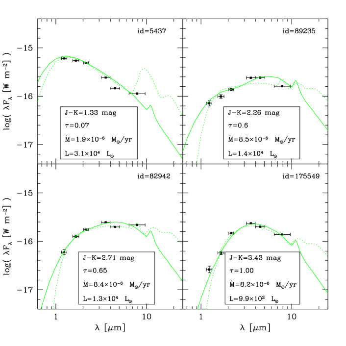
Figure 1: Example SEDs of presumed carbon stars. The horizontal ”errorbars” on the data represent the width of the photometric passbands. The best matching SEDs modelled with dusty are shown with solid lines. For comparison, the best matching fits using silicates are shown with dotted lines.

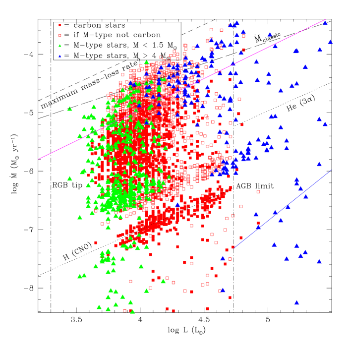
Figure 2: Mass–loss rate vs. luminosity, modelled with dusty for low–mass AGB stars (green triangles), intermediate–mass carbon stars (red squares) and massive AGB stars and RSGs (blue triangles). The open red squares show the results if the presumed carbon stars are presumed to be oxygen–rich instead. The vertical dash–dotted lines mark the tip luminosity of the first ascent red giant branch (RGB) and the classical limit of the most massive AGB stars (excluding the effects of Hot Bottom Burning). The dotted lines trace the mass–consumption rates by shell hydrogen burning (CNO cycle) on the AGB and core helium burning (triple–$\alpha$ reaction) in RSGs. The dashed lines trace the limits to the mass–loss rate in dust-driven winds due to single scattering (classic) and multiple scattering (maximum?; see van Loon et al. 1999). The magenta line traces the fit to the mass–loss rate vs. luminosity presented in Goldman et al. (2017), whilst the blue line traces the relation found by Verhoelst et al. (2009) for Galactic RSGs.

Spectral energy distributions (SEDs) contain information about the stellar luminosity, temperature, metal content, surface gravity and extinction. If sampled over a sufficient range in wavelength, employing accurate stellar spectral templates allows to retrieve some or all of these parameters. To model SEDs of WFCAM variables we used the publicly available dust radiative transfer code DUSTY (Ivezić & Elitzur 1997). All variables with at least two measurements in near–IR bands (K_s and J and/ or H) and two mid–IR bands (3.6, 4.5 and/or 8 $\mu$m) were modelled ($\sim$ 2000 stars). DUSTY calculates the radiation transport in a dusty envelope. We fixed the input temperatures of the star and of the dust at the inner edge of the circumstellar envelope, at 3000 and 900 K, respectively. The density structure is assumed to follow from the analytical approximation for radiatively driven winds (Ivezić, Nenkova & Elitzur 1999). This obviates the need to assume or measure the outflow velocity, as it is implicit in the relation between luminosity, optical depth, gas–to–dust mass ratio and mass–loss rate. We used amorphous carbon dust (Hanner 1988) and a small amount (15 per cent) of silicon carbide (Pégourié 1988) for carbon stars, and astronomical silicates (Draine & Lee 1988) for M–type stars (Fig. 1). Because a sub–set of AGB stars, carbon stars have a different type of circumstellar dust, we must try to identify which stars are likely to be carbon stars. In the absence of spectroscopic confirmation for most of these, and the limited constraints we have from photometry, we resort to making use of theoretical expectations. Correcting the observed colours for the effect of circumstellar dust, we obtain an intrinsic K–band brightness. Using stellar evolution models (Marigo et al. 2017) we convert this into a birth mass, given that these are highly evolved stars that will not evolve much in luminosity. The mass range for AGB stars to become carbon stars spans $\sim 1.5$–4 M_⊙.

5.1 Mass–loss rate

For our complete sample (Javadi et al. 2015), some dependence of mass–loss rate on luminosity is seen (Fig. 2); the maximum mass–loss rate increases with luminosity and the highest mass–loss rates are generally achieved by the most luminous, most massive large–amplitude variable stars. This confirms earlier studies in the central region of M 33 (Javadi et al. 2013) and in the Magellanic Clouds (Srinivasan et al. 2009). The mass–loss rates for M–type AGB stars and RSGs are similar to those found in the Solar Neighbourhood (a few $\times 10^{-5}$ and $10^{-7}$–$10^{-4}$ M_⊙ yr^-1, respectively; Jura & Kleinmann 1989). The mass–loss rates for presumed carbon stars are also in good agreement with those found in the Milky Way (a few $\times 10^{-5}$ M_⊙ yr^-1; Whitelock et al. 2006) and in the Magellanic Clouds ($\sim 10^{-5}$ M_⊙ yr^-1; Gullieuszik et al. 2012).

It is reassuring to see that the RSGs (certainly stars well above the AGB limit of $\log L/L_{\odot}=4.73$ – Wood, Bessell & Fox (1983)) are generally oxygenous; that the least luminous stars are too, and that the maximum mass–loss rate increases with luminosity (in fact rather steeply). Oxygenous stars around – or slightly fainter than – the AGB limit with very high mass–loss rates are probably massive AGB stars, the equivalent of (most of) the OH/IR stars that are found in the LMC (Marshall et al. 2004).

6 On going works and conclusion remarks

Comparison of the total mass return rate from dusty evolved stars across the galactic disc of M 33 ($\approx$0.1 M_⊙yr^-1; Fig. 2) and recent star formation rate ( $\xi=0.45\pm 0.10$ M_⊙yr^-1; Javadi et al. 2017), suggests that for star formation to continue beyond the next Gyr or so, gas must flow into the disc of M 33, via cooling flows from the circum–galactic medium and/or by inward migration from gas reservoirs in the outskirts of the disc (Javadi et al. in prep).

In order to gain a comprehensive understanding of galaxy formation and evolution in the Local Group, recently we have conducted an optical monitoring survey of the majority of nearby dwarf galaxies with Isaac Newton Telescope (INT) to identify LPVs (Saremi et al. 2019, 2020, 2021; Navabi el al. 2021). This research is very important from both theoretical and observational perspectives: First, it will give an unprecedented map of the temperature and radius variations as a function of luminosity and metallicity for mass-losing stars at the end of their evolution, which places important constraints on stellar evolution models and which is a vital ingredient in the much sought-after description of the mass-loss process. Second, from observational prospective, this research will gather independent diagnostics of the SFHs of different types of dwarf galaxies found in different environments, which help build a detailed picture of galaxy evolution in the nearby galaxies.

References

- [Davidge (2000)] Davidge T., 2000, AJ, 119, 748
- [Davidge (2018)] Davidge T., 2018, ApJ, 856, 129
- [Draine & Lee (1984)] Draine B. T., Lee H. M., 1984, ApJ, 285, 89
- [Georgy (2012)] Georgy C., 2012, A&A, 538, L8
- [Georgy et al.(2012)] Georgy C., Ekström S., Meynet G., Massey P., Levesque E. M., Hirschi R., Eggenberger P., Maeder A., 2012, A&A, 542, A29
- [Goldman et al.(2017)] Goldman S. R. et al., 2017, MNRAS, 465, 403
- [Goldman et al. (2019)] Goldman S. R., 2019, ApJ, 877, 49
- [Gullieuszik et al.(2012)] Gullieuszik M. et al., 2012, A&A, 537A, 105
- [Hanner (1988)] Hanner M. S., 1988, NASA Conf. Pub. 3004, 22
- [Ita et al. (2004)] Ita Y., et al. 2004, MNRAS, 353, 705
- [Ivezić & Elitzur (1997)] Ivezić Ž, Elitzur M., 1997, MNRAS, 287, 799
- [Ivezić, Nenkova & Elitzur (1999)] Ivezić Ž, Nenkova M., Elitzur M., 1999, dusty User Manual (University of Kentucky)
- [Javadi et al. (2011)] Javadi A., van Loon J. Th., Mirtorabi M. T., 2011, MNRAS, 414, 3394
- [Javadi et al. (2013)] Javadi A., van Loon J. Th., Khosroshahi H. G., Mirtorabi M. T., 2013, MNRAS, 432, 2824
- [Javadi et al. (2015)] Javadi A., Saberi M., van Loon J. Th., Khosroshahi H. G., Golabatooni N., Mirtorabi M. T., 2015, MNRAS, 447, 3973
- [Javadi et al. (2017)] Javadi A., van Loon J. Th., Khosroshahi H. G., Tabatabaei F., Hamedani Golshan R., Rashidi M., 2017, MNRAS, 464, 2103
- [Jura & Kleinmann (1989)] Jura M., Kleinmann S. G., 1989, ApJ, 341, 359
- [Levesque et al. (2005)] Levesque E. M., Massey P., Olsen K. A. G., Plez B., Josselin E., Maeder A., Meynet G., 2005, ApJ, 628, 973
- [Marigo et al. (2017)] Marigo P. et al., 2017, ApJ, 835, 19
- [Marshall et al.(2004)] Marshall J. R., van Loon J. Th., Matsuura M., Wood P. R., Zijlstra A. A., Whitelock P. A., 2004, MNRAS, 355, 1348
- [McQuinn et al.(2007)] McQuinn K. B. W. et al., 2007, ApJ, 664, 850
- [Navabi et al. (2021)] Navabi M., Saremi E., Javadi A., Noori M., van Loon J. Th., Khosroshahi H. G., McDonald I., Alizadeh M., Danesh A., Gozaliasl G., Molaeinezhad A., Parto T., Raouf M., 2021, ApJ, 910, 127
- [Pégourié (1988)] Pégourié B., 1988, A&A, 194, 335
- [Saremi et al. (2019)] Saremi E., Javadi A., van Loon J. Th., Khosroshahi H. G., Rezaeikh S., Hamedani Golshan R., Hashemi S. A., 2019, Proceedings of IAU Symposium, 344, 125
- [Saremi et al. (2020)] Saremi E. et al., 2020, ApJ, 894, 135
- [Saremi et al. (2021)] Saremi E, Javadi A., Navabi M., van Loon J. Th., Khosroshahi H. G., Bojnordi Arbab B., McDonald I., 2021, ApJ, 923, 164
- [Srinivasan et al.(2009)] Srinivasan S. et al., 2009, AJ, 137, 4810
- [van Loon et al.(1999)] van Loon J. Th., Groenewegen M. A. T., de Koter A., Trams N. R., Waters L. B. F. M., Zijlstra A. A., Whitelock P. A., Loup C., 1999, A&A, 351, 559
- [van Loon et al.(2005)] van Loon J. Th., Cioni M.-R. L., Zijlstra A. A., Loup C., 2005, A&A, 438, 273
- [van Loon et al.(2006)] van Loon J. Th., Marshall J. R., Cohen M., Matsuura M., Wood P. R., Yamamura I., Zijlstra A. A., 2006, A&A, 447, 971
- [Verhoelst et al.(2009)] Verhoelst T., Van der Zypen N., Hony S., Decin L., Cami J., & Eriksson K., 2009, A&A, 498, 127
- [Whitelock et al.(2006)] Whitelock P. A., Feast M. W., Marang F., Groenewegen M. A. T., 2006, MNRAS, 369, 751
- [Wood, Bessell & Fox (1983)] Wood P. R., Bessell M. S., Fox M. W., 1983, ApJ, 272, 99
- [Wood (2000)] Wood P. R., 2000, PASA, 17, 18
- [Yuan (2018)] Yuan W., Macri L. M., Javadi A., Lin Z., Huang J. Z., 2018, AJ, 156, 112