Abstract

Assuming Newton’s law of cooling, the propagation and structure of isothermal acoustic shocks are studied under four different viscosity laws. Employing both analytical and numerical methods, 1D traveling wave solutions for the velocity and density fields are derived and analyzed. For each viscosity law considered, expressions for both the shock thickness and the asymmetry metric are determined. And, to ensure that isothermal flow is achievable, upper bounds on the associated Mach number values are derived/computed using the isothermal version of the energy equation.

Keywords: Artificial viscosity, Dispersed shocks, Isothermal propagation,
Newton’s law of cooling  Traveling wave solutions

1 Introduction

In a celebrated paper published in 1849, Stokes [1] appears to have been the first to consider the impact of shear viscosity on the 1D propagation of linear acoustic waves in gases. Two years later, Stokes [2] went on to examine the propagation of linear, time-harmonic, acoustic plane waves in a gas whose only loss mechanism is its ability to radiate heat to its surroundings, the process of which he modeled using Newton’s law of cooling; see Appendix A. In 1910, Rayleigh [3, pp. 270–271] presented a partial analysis of the isothermal propagation of an infinite (1D) “wave of condensation” in a constant viscosity, but thermally non-conducting, gas, the process of radiation being invoked to maintain the flow’s isothermal nature. Later, Lamb (see, e.g., Ref. [4, § 360]) and, in 1953, Truesdell [5, p. 687] generalized Stokes’ [2] radiant propagation model to include the effects of both viscosity and thermal conduction. In 2004, LeVeque [6] employed the assumption of isothermal flow to investigate 1D “delta shocks” in lossless perfect gases; because he did not consider the energy equation, however, LeVeque’s analysis, like Rayleigh’s [3, pp. 270–271], must be considered as only partially complete.

The primary aim of the present study is to not only complete, but also extend Rayleigh’s analysis, wherein only the equation of motion (EoM) for the density field was derived and integrated, by considering the effects of various viscosity laws on the propagation and structure of acoustic shocks in the setting of the isothermal piston problem. Specifically, we determine and analyze 1D traveling wave solutions (TWS)s, under the assumption that the temperature of the gas in question is held constant, based on the following four viscosity laws: (i) constant shear viscosity (i.e., the case considered in Ref. [3, pp. 270–271]), (ii) shear viscosity proportional to mass density, (iii) von Neumann–Richtmyer artificial viscosity, and (iv) Evans–Harlow–Longley artificial viscosity. These particular laws were selected primarily because all lead to model systems that are amiable to study by analytical means.

To provide a mechanism for achieving isothermal flow, we, like Rayleigh, invoke the process of radiation, which like Stokes [2] we model via Newton’s law of cooling. To ensure that isothermal flow is not only mathematically but also physically possible, under each of the four cases considered, we also determine, based on the full form of the isothermal energy equation, the upper bound on the range of (piston) Mach number values corresponding to each case.

In the next section, we begin our investigation with a review of the thermodynamics of perfect gases and the formulation of our governing system of equations.

Remark 1: As Chandrasekhar [7, Chap. II] notes, isothermal flow is a particular type of polytropic process—one quantified by $\gamma^{\prime}=1$, $n=\infty$, where $\gamma^{\prime}$, $n$ are used by Chandrasekhar to represent the polytropic exponent and polytropic index, respectively; see Ref. [7, pp. 41–44].

2 Formulation of mathematical model

2.1 Thermodynamical aspects of perfect gases

As defined by Thompson [8], a perfect gas is one in which $p(>0)$, the thermodynamic pressure, $\rho(>0)$, the mass density, and $\vartheta(>0)$, the absolute temperature, obey the following special case of the ideal gas law [8, § 2.5]:

$$p=c_{\rm v}(\gamma-1)\rho\vartheta\qquad(c_{\rm p},c_{\textrm{v}}:=\text{const.}).$$ (1)

Here, $c_{\rm p}>c_{\rm v}>0$ are the specific heats at constant pressure and constant volume, respectively, and $\gamma=c_{\rm p}/c_{\textrm{v}}$, where $\gamma\in(1,5/3]$ in the case of perfect gases. Furthermore, a zero (“0”) subscript attached to a field variable identifies the uniform equilibrium state value of that variable; i.e., in the present investigation, the gas is assumed to be homogeneous when in its equilibrium state.

With regard to the perfect gas assumption we note that the equilibrium state values of the adiabatic and isothermal sound speeds in the gas are given by

$$c_{0}=\sqrt{c_{\rm p}(\gamma-1)\vartheta_{0}}$$ (2)

and

$$b_{0}=c_{0}\gamma^{-1/2}=\sqrt{c_{\textrm{v}}(\gamma-1)\vartheta_{0}},$$ (3)

respectively, where we observe that $b_{0}\in(0,c_{0})$. That is, $c_{0}$ and $b_{0}$ are, respectively, the speeds of infinitesimal-amplitude acoustic signals under the adiabatic and isothermal assumptions; see, e.g., Ref. [4, § 278], wherein $b_{0}$ is referred to as the “Newtonian velocity of sound”.

In this study we will also make use of the thermodynamic axiom known as the Gibbs relation [8, p. 58], which in the case of a perfect gas can be written as

$$\vartheta\,\textrm{d}\eta=\textrm{d}E-c_{\rm v}(\gamma-1)\vartheta\rho^{-1}\textrm{d}\rho\qquad(\text{perfect gases}),$$ (4)

where $\eta$ is the specific entropy and $E$ is the specific internal energy. Here, we note for later reference the relations

$$E=c_{\rm v}\vartheta=H/\gamma\qquad(\text{perfect gases}),$$ (5)

where $H$ is the specific enthalpy.

2.2 Navier–Stokes–Fourier system in 1D

For the 1D flow of a perfect gas along the $x$-axis of a Cartesian coordinate system, the Navier–Stokes–Fourier (NSF) system [9, p. 513] can, assuming the absence of all body forces and that the ratio $\mu_{\rm b}/\mu$ is constant, be written in the following form:

$$\frac{\partial\rho}{\partial t}+u\frac{\partial\rho}{\partial x}+\rho\frac{\partial u}{\partial x} =0,$$ (6a)

$$\rho\left(\frac{\partial u}{\partial t}+u\frac{\partial u}{\partial x}\right)+\rho c_{\rm p}\frac{\partial\vartheta}{\partial x} =\rho\vartheta\frac{\partial\eta}{\partial x}$$

$$\!\!\!\!+\textrm{\Large{$\upsilon$}}\frac{\partial}{\partial x}\!\left(\mu\frac{\partial u}{\partial x}\right)\!,$$ (6b)

$$\rho\vartheta\left(\frac{\partial\eta}{\partial t}+u\frac{\partial\eta}{\partial x}\right)-\Phi =\rho r-\frac{\partial q}{\partial x},$$ (6c)

$$q =-K\frac{\partial\vartheta}{\partial x},$$ (6d)

$$c_{\rm v}\ln(\vartheta/\vartheta_{0})-c_{\rm v}(\gamma-1)\ln(\rho/\rho_{0}) =\eta-\eta_{0},$$ (6e)

where $p=p(x,t)$, $\rho=\rho(x,t)$, $\vartheta=\vartheta(x,t)$, and $\eta=\eta(x,t)$ under this flow geometry. In Sys. (6), ${\bf u}=(u(x,t),0,0)$ and ${\bf q}=(q(x,t),0,0)$ are, respectively, the velocity and heat flux vectors; $\mu(>0)$ is the shear (or dynamic) viscosity; $\textrm{\Large{$\upsilon$}}=\tfrac{4}{3}+\mu_{\rm b}/\mu$ is the viscosity number, where $\mu_{\rm b}(\geq 0)$ is the bulk viscosity; $K(>0)$ is the thermal conductivity; and $r$, which carries units of W/kg (i.e., m²/s³), represents the external rate of supply of heat per unit mass. Moreover, $\Phi$, the dissipation function [8, 9], here takes the form

$$\Phi=\mu\textrm{\Large{$\upsilon$}}\left(\partial u/\partial x\right)^{2};$$ (7)

Eq. (6e) follows from integrating Eq. (4) after substituting in $E$ from Eq. (5); and we note that the pressure gradient term that would normally have appeared in Eq. (6b) was eliminated using the relevant 1D special case of the thermodynamic relation [8, p. 71]

$$\rho^{-1}\nabla p=\nabla H-\vartheta\nabla\eta.$$ (8)

In what follows we consider the compressive version of the classic (1D) piston problem. That is, the piston, whose face we take to be thermally insulated, is located at $x=-\infty$ and moving to the right with constant speed $u_{\rm p}(>0)$ while the gas at $x=+\infty$ is in its equilibrium state. In this regard we also observe that, since the piston’s motion is strictly compressive, it follows that $u\in[0,u_{\rm p}]$ and $\partial u/\partial x\leq 0$ will always hold under the assumed flow geometry.

Additionally, we will invoke the assumption

$$\mu_{\rm b}=0,$$ (9)

which of course is Stokes’ hypothesis [8, 9]. Here, we stress that Eq. (9), which in the case of air, e.g., is only an approximation [8, Table 1.1], will not be a limitation on our analysis. This is because our numerical results will focus exclusively on the (monatomic) gas Ar — one for which Eq. (9) has been shown, by both theory and experiment, to hold exactly; see, e.g., Refs. [11, 12].

2.3 Isothermal piston problem

Assuming hereafter that the flow is isothermal, i.e., $\vartheta\equiv\vartheta_{0}$, we find that Eq. (1) (i.e., our EoS) and the constitutive relations given in Eqs. (6d) and (6e) reduce, respectively, to

$$p=b_{0}^{2}\rho=p_{0}\rho/\rho_{0},$$ (10)

which is simply Boyle’s law [3];

$$q=0,$$ (11)

since $\partial\vartheta_{0}/\partial x=0$; and

$$\eta-\eta_{0}=-c_{\textrm{v}}(\gamma-1)\ln(\rho/\rho_{0}),$$ (12)

which is the isothermal special case of Eq. (6e).

On carrying out these substitutions, followed by the use of Eqs (6a), (7), and (9), Sys. (6) is reduced to

$$\frac{\partial\rho}{\partial t}+u\frac{\partial\rho}{\partial x}+\rho\frac{\partial u}{\partial x} =0,$$ (13a)

$$\rho\left(\frac{\partial u}{\partial t}+u\frac{\partial u}{\partial x}\right)+b_{0}^{2}\frac{\partial\rho}{\partial x}-\frac{4}{3}\frac{\partial}{\partial x}\!\left(\mu\frac{\partial u}{\partial x}\right) =0,$$ (13b)

$$\vartheta_{0}+\frac{b_{0}^{2}}{c_{\rm v}\varkappa_{0}}\frac{\partial u}{\partial x}-\frac{(4/3)}{c_{\rm v}\varkappa_{0}}\left(\frac{\mu}{\rho}\right)\!\left(\frac{\partial u}{\partial x}\right)^{2} =\vartheta_{\rm e},$$ (13c)

where our adoption of Stokes’ hypothesis yields $\textrm{\Large{$\upsilon$}}=4/3$.

In Eq. (13c), we have taken $r$ to be given by the isothermal special case of Newton’s law of cooling, viz.:

$$r=-c_{\rm v}\varkappa_{0}(\vartheta_{0}-\vartheta_{\rm e}),$$ (14)

where $\varkappa_{0}(>0)$, the “velocity of cooling” [2, p. 307], carries units of 1/s; see also Ref. [5, pp. 651, 687]. Here, $\vartheta_{\rm e}=\vartheta_{\rm e}(x,t)$, the temperature of the surrounding environment, is an additional dependent variable that is controllable by the experimenter based on “output” from Eq. (13c). This, of course, is necessary because the gas must be able to radiate away the resulting heat of its compression, at a rate that cannot be assumed constant, if our assumption of isothermal flow is to be satisfied + maintained. (Note that the ability of the gas to conduct heat plays no role under the isothermal assumption.) In this regard, we have adopted the assumptions stated by Rayleigh [10, p. 28] regarding the physical and thermal characteristics of the enclosing cylinder.

2.4 Viscosity laws: Classical and artificial

In this subsection we give the precise statement of the four viscosity laws mentioned in Section 1. Note that the first two stem from classical continuum theory while the latter two are of the artificial type.

1. Constant shear viscosity:

   $$\mu=\mu_{0};$$ (15)

   recall, this is the case considered in Ref. [3, pp. 270–271]; it is also the exact form of $\mu$ for the current (i.e., isothermal) problem under the kinetic theory of gases.

2. Shear viscosity proportional to mass density:

   $$\mu=\nu_{0}\rho;$$ (16)

   see Refs. [11, § 12.11] and [13].

3. von Neumann–Richtmyer (vNR) artificial viscosity:

   $$\mu=-\mathfrak{b}_{\rm iii}^{2}\lambda_{0}^{2}\rho\!\left(\frac{\partial u}{\partial x}\right)\!;$$ (17)

   see Refs. [14] and [15, § V-D-1].

4. Evans–Harlow–Longley (EHL) artificial viscosity:

   $$\mu=\tfrac{1}{2}\mathfrak{b}_{\rm iv}\lambda_{0}\rho u;$$ (18)

   see Refs. [15, § V-D-2], [16, p. 16], and [17, p. 11].

Here, $\mu_{0}$ and $\nu_{0}=\mu_{0}/\rho_{0}$ represent, respectively, the (constant) equilibrium state values of the shear and kinematic viscosity coefficients; in the case of hard-sphere molecules we have, according to the kinetic theory of gases [8, § 2.7],

$$\mu_{0}=\tfrac{5}{32}\pi\rho_{0}\bar{c}_{0}\lambda_{0},$$ (19)

an expression which also follows on setting “$\delta$” in Ref. [18, Eq. (9b)] equal to $5\pi/32\approx 0.491$; we let $\lambda_{0}(>0)$ denote the equilibrium state value of the molecular mean-free-path (see, e.g., Refs. [18, p. 680] and [8, pp. 95–97]); the equilibrium state value of the mean molecular speed is given by [8, p. 108]

$$\bar{c}_{0}=c_{0}\sqrt{8/(\gamma\pi)}=b_{0}\sqrt{8/\pi};$$ (20)

and $\mathfrak{b}_{\rm iii}(>0)$ and $\mathfrak{b}_{\rm iv}(>0)$ are adjustable dimensionless parameters [15, § V-D-1].

Lastly, since our investigation is to be carried out primarily by analytical methodologies, and we seek an approach that would allow one to compare/contrast these four cases in a consistent manner, we have taken $\Delta x=\lambda_{0}$, where $\Delta x$ is the spatial mesh increment used in the usual statements of both the vNR and EHL laws. And with regard to $\lambda_{0}$ we record here, for later reference, the expression

$$\lambda_{0}=\frac{16\nu_{0}}{b_{0}\sqrt{50\pi}},$$ (21)

which is easily obtained after eliminating $\bar{c}_{0}$ between Eqs. (19) and (20), and we note that $16/\sqrt{50\pi}\approx 1.277$.

3 Traveling wave reduction

3.1 Ansatzs and wave variable

Invoking the traveling wave assumption, we set

$$u(x,t)=f(\zeta),\quad\rho(x,t)=g(\zeta),\quad\vartheta_{\rm e}(x,t)=\Theta_{\rm e}(\zeta),$$ (22)

where $\zeta:=x-vt$ is the wave (i.e., similarity) variable, and where the parameter $v(>0)$ will be seen to represent the speed of the resulting shocks. On substituting the above ansatzs into Sys. (13), the latter is reduced to the following system of ODEs:

$$\frac{\textrm{d}}{\textrm{d}\zeta}\left(-vg+fg\right)=0,$$ (23a)

$$g(-v+f)f^{\prime}+b_{0}^{2}g^{\prime}-\frac{4}{3}\frac{\textrm{d}}{\textrm{d}\zeta}\left(\mu f^{\prime}\right)=0,$$ (23b)

$$\vartheta_{0}+\left(\frac{b_{0}^{2}}{c_{\rm v}\varkappa_{0}}\right)\!f^{\prime}-\frac{(4/3)}{c_{\rm v}\varkappa_{0}}\left(\frac{\mu}{g}\right)\!\left(f^{\prime}\right)^{2}=\Theta_{\rm e},$$ (23c)

where a prime denotes $\textrm{d}/\textrm{d}\zeta$.

This system is to be integrated subject to the asymptotic conditions

$$f\to u_{\rm p},\quad f^{\prime}\to 0\qquad(\zeta\to-\infty),g\to\rho_{0},\quad f,f^{\prime}\to 0\qquad(\zeta\to+\infty),$$ (24)

which of course correspond to a shock moving to the right; recall that $v>0$.

3.2 Shock speed and associated ODE

Using the fact that Eq. (23a) integrates to

$$g=\frac{\rho_{0}v}{v-f},$$ (25)

allows us to, in turn, integrate Eq. (23b):

$$-\rho_{0}vf+b_{0}^{2}g-(4\mu/3)f^{\prime}=b_{0}^{2}\rho_{0},$$ (26)

where the resulting constants of integration were found to be $\mathcal{K}_{1}=-\rho_{0}v$ and $\mathcal{K}_{2}=\rho_{0}b_{0}^{2}$, respectively. Now eliminating $g$ between the former and latter equations yields

$$(4\mu/3)(v-f)f^{\prime}=\rho_{0}[(b_{0}^{2}-v^{2})f+vf^{2}],$$ (27)

i.e., a Riccati type equation. Employing the asymptotic conditions once again leads us to consider

$$v^{2}-b_{0}^{2}=u_{\rm p}v,$$ (28)

a quadratic whose only positive root is

$$v=\frac{u_{\rm p}+\sqrt{u_{\rm p}^{2}+4b_{0}^{2}}}{2}=\tfrac{1}{2}u_{\rm p}\left(1+\sqrt{1+4\textrm{Ma}^{-2}}\,\right)\!,$$ (29)

where $\textrm{Ma}=u_{\rm p}/b_{0}$ is the piston Mach number.

With these results in-hand, we can reduce Sys. (23) to the two-equation system

$$(4\mu/3)(v-f)f^{\prime}+\rho_{0}vu_{\rm p}(1-f/u_{\rm p})f=0,$$ (30a)

$$\vartheta_{0}-\left(\frac{b_{0}^{2}}{c_{\rm v}\varkappa_{0}}\right)\!|f^{\prime}|-\frac{(4\mu/3)}{c_{\rm v}\varkappa_{0}}\left(\frac{v-f}{\rho_{0}v}\right)\!\left|f^{\prime}\right|^{2}=\Theta_{\rm e}.$$ (30b)

Eq. (30a) is the associated ODE of our traveling wave analysis; in the next four sections, we shall integrate it, under each of the aforementioned cases of $\mu$, subject to the wave-front condition $f(0)=\tfrac{1}{2}u_{\rm p}$.

3.3 Shock thicknesses, $Q$-metric, and jump amplitudes

Employing the notation

$$f(\pm\infty):=\lim_{\zeta\to\pm\infty}f(\zeta),\qquad g(\pm\infty):=\lim_{\zeta\to\pm\infty}g(\zeta),$$ (31)

we define the shock thickness of the velocity profile by

$$\ell_{j}:=\frac{f(-\infty)-f(+\infty)}{\max\big{|}f^{\prime}(\zeta)\,\big{|}}=\frac{u_{\rm p}}{|f^{\prime}(\zeta_{j}^{\bullet})|},$$ (32)

a definition which Morduchow and Libby [18, p. 680] attribute to Prandtl, and that of the density profile by

$$l_{j}:=\frac{g(-\infty)-g(+\infty)}{\max\big{|}g^{\prime}(\zeta)\,\big{|}}=\left(\frac{2}{-1+\sqrt{1+4\textrm{Ma}^{-2}}}\right)\frac{\rho_{0}}{|g^{\prime}(\zeta_{j}^{*})|}.$$ (33)

Here, $\zeta=\zeta_{j}^{\bullet}$ and $\zeta=\zeta_{j}^{*}$ denote the relevant stationary points of $f^{\prime}$ and $g^{\prime}$, respectively, i.e., $f^{\prime\prime}(\zeta_{j}^{\bullet})=0$ and $g^{\prime\prime}(\zeta_{j}^{*})=0$; the subscript $j$ represents the number [i.e., (i)–(iv)] of the case under consideration; and with regard to Eq. (33) we note the following:

$$g^{\prime}(\zeta)=\frac{\rho_{0}vf^{\prime}}{(v-f)^{2}}=-\frac{3\rho_{0}^{2}v^{2}(u_{\rm p}-f)f}{4\mu(v-f)^{3}}$$ (34)

and

$$g(-\infty)=\frac{\rho_{0}v}{v-u_{\rm p}}=\rho_{0}\left(\frac{1+\sqrt{1+4\textrm{Ma}^{-2}}}{-1+\sqrt{1+4\textrm{Ma}^{-2}}}\right)>g(+\infty)=\rho_{0}.$$ (35)

We also define the $Q$- (or asymmetry) metric

$$Q(\textrm{Ma})=\frac{\displaystyle\int_{-\infty}^{0}[1-R(\zeta)]\,\textrm{d}\zeta}{\displaystyle\int_{0}^{+\infty}R(\zeta)\,\textrm{d}\zeta},$$ (36)

where

$$R(\zeta)=\frac{g(\zeta)-\rho_{0}}{g(-\infty)-\rho_{0}}\implies\lim_{\zeta\to\mp\infty}R(\zeta)=1,0,$$ (37)

respectively. As Schmidt [19, p. 369] points out, not only is $Q$ a “sensitive measure of asymmetry”, but it also complements the shock thickness as a characterizing metric since the latter “fails to give sufficiently detailed information about [shock] structure; . . .” [19, p. 361]. In Section 8.3 (below), we use $Q$ to quantify the degree of asymmetry exhibited by each of the four $g$ vs. $\zeta$ profiles studied below.

Lastly, we define, following Morro [20] and Straughan [21], the amplitude of the jump in a function $\mathfrak{F}=\mathfrak{F}(\zeta)$ across the plane $\zeta=\zeta_{\rm d}$ as

$$[\![\mathfrak{F}]\!]\Big{|}_{\zeta_{\rm d}}=\lim_{\zeta\to\zeta_{\rm d}^{-}}\mathfrak{F}(\zeta)-\lim_{\zeta\to\zeta_{\rm d}^{+}}\mathfrak{F}(\zeta),$$ (38)

where it is assumed that both limits exist and that they are different. Here, we call attention to the fact that $[\![\mathfrak{F}]\!]$ is positive (resp. negative) when the jump in $\mathfrak{F}$ is from higher (resp. lower) to lower (resp. higher) values.

4 Constant shear viscosity case

Recall that under Case (i), $\mu=\mu_{0}$; consequently, Eq. (30a) becomes

$$(4\nu_{0}/3)(v-f)f^{\prime}+vu_{\rm p}(1-f/u_{\rm p})f=0,$$ (39)

which on setting $\mathcal{F}(\zeta)=-1+(2/u_{\rm p})f(\zeta)$ is reduced to

$$(k+\mathcal{F})\mathcal{F}^{\prime}=\frac{3v}{4\nu_{0}}(1-\mathcal{F}^{2}).$$ (40)

This ODE, like the former, is a particularly simple special case of Abel’s equation [24]; as such, it is easily integrated and yields the exact, but generally implicit, TWS:

$$\left(\frac{3v}{4\nu_{0}}\right)\zeta=k\tanh^{-1}(\mathcal{F})-\frac{1}{2}\ln(1-\mathcal{F}^{2})\qquad(|\mathcal{F}|<1).$$ (41)

Here, the constant of integration is zero, by way of the fact that $f(0)=u_{\rm p}/2$ implies $\mathcal{F}(0)=0$; we have set

$$k=1-2v/u_{\rm p}=-\sqrt{1+4\textrm{Ma}^{-2}};$$ (42)

and we note for later reference (in Appendix B) that Eq. (41) can also be expressed as

$$\left(\frac{3v}{2\nu_{0}}\right)\zeta=(k-1)\ln(1+\mathcal{F})-(k+1)\ln(1-\mathcal{F})\qquad(|\mathcal{F}|<1).$$ (43)

Because $k<-1$, the integral curves described by Eq. (41) can only take the form of fully dispersed shocks, also referred to by some as kinks; see, e.g., Ref. [25, § 5.2.2]. For this velocity traveling wave profile, therefore, we can show that the shock thickness is given by

$$\ell_{\rm i}=\frac{8(\nu_{0}/b_{0})\textrm{Ma}}{3\!\left(\textrm{Ma}+\sqrt{4+\textrm{Ma}^{2}}\,\right)\left(-2+\sqrt{4+\textrm{Ma}^{2}}\,\right)},$$ (44)

to which corresponds the stationary point

$$\zeta_{\rm i}^{\bullet}=-\left(\frac{4\nu_{0}}{3v}\right)\Bigg{[}\sqrt{1+4\textrm{Ma}^{-2}}\times\tanh^{-1}\left(\frac{-2+\sqrt{4+\textrm{Ma}^{2}}}{\textrm{Ma}}\,\right)$$

$$+\frac{1}{2}\ln\left(\frac{-8+4\sqrt{4+\textrm{Ma}^{2}}}{\textrm{Ma}^{2}}\,\right)\Bigg{]};$$

here, we observe that

$$\mathcal{F}(\zeta_{\rm i}^{\bullet})=\mathcal{F}_{\rm i}^{\bullet}:=|k|-\sqrt{k^{2}-1}=|k|-2/\textrm{Ma},$$ (45)

which when related back to $f$ yields

$$f(\zeta_{\rm i}^{\bullet})=f_{\rm i}^{\bullet}:=\tfrac{1}{2}u_{\rm p}\left(1+|k|-2/\textrm{Ma}\right).$$ (46)

In order to determine $l_{\rm i}$, we must first determine the (only) positive root of $\Pi(Y)=0$, where

$$\Pi(Y)=Y^{2}+2|k|Y-3.$$ (47)

This quadratic arises when we attempt to solve $g^{\prime\prime}(\zeta)=0$ after expressing it in terms of $\mathcal{F}$ and simplifying, i.e., when seeking the solution of

$$[3(1-\mathcal{F}^{2})+2\mathcal{F}(k+\mathcal{F})]\mathcal{F}^{\prime}=0,$$ (48)

which we do subject to the constraint $|\mathcal{F}|\in(0,1)$. Denoting the aforementioned root by $Y=\mathcal{F}_{\rm i}^{*}$, it is not difficult to establish that

$$\mathcal{F}(\zeta_{\rm i}^{*})=\mathcal{F}_{\rm i}^{*}:=-|k|+\sqrt{k^{2}+3},$$ (49)

which when related back to $f$ yields

$$f(\zeta_{\rm i}^{*})=f_{\rm i}^{*}:=\tfrac{1}{2}u_{\rm p}\left(1-|k|+\sqrt{k^{2}+3}\,\right)\!,$$ (50)

where the stationary point of the corresponding $g^{\prime}$ vs. $\zeta$ profile is given by

$$\zeta_{\rm i}^{*}=\left[\frac{8\nu_{0}}{3u_{\rm p}(|k|+1)}\right]\!\left\{k\tanh^{-1}(\mathcal{F}_{\rm i}^{*})-\tfrac{1}{2}\ln\left[1-(\mathcal{F}_{\rm i}^{*})^{2}\right]\right\}\!.$$ (51)

With Eq. (49) in hand and observing that, under Case (i), Eq. (34) becomes

$$g^{\prime}(\zeta)=-\frac{3\rho_{0}v^{2}(u_{\rm p}f-f^{2})}{4\nu_{0}(v-f)^{3}}=\left(\frac{3v^{2}\rho_{0}}{2u_{\rm p}\nu_{0}}\right)\!\frac{(1-\mathcal{F}^{2})}{(k+\mathcal{F})^{3}},$$ (52)

the density profile is seen to admit the shock thickness

$$l_{\rm i}=\frac{16(\nu_{0}/b_{0})}{3\textrm{Ma}(|k|-1)(|k|+1)^{2}}\left\{\frac{|k+\mathcal{F}_{\rm i}^{*}|^{3}}{1-(\mathcal{F}_{\rm i}^{*})^{2}}\right\}.$$ (53)

Remark 2: Small-$|\zeta|$ and large-$|\zeta|$ approximations to $\mathcal{F}$ can easily be determined from the corresponding expressions for “$\mathcal{U}$” given in Ref. [25, Remark 9], wherein “$\xi$” plays the role of $\zeta$. Mention should also be made of the explicit, but approximate, result [25, Remark 10]

$$f(\zeta)\approx\tfrac{1}{2}u_{\rm p}\left[1-\tanh\left(2\zeta/\hat{\ell}_{\rm i}\right)\right]\qquad(\textrm{Ma}\ll 1),$$ (54)

for which the shock thickness is $\hat{\ell}_{\rm i}=16\nu_{0}/(3b_{0}\textrm{Ma})$, and we note that $\textrm{Ma}\ll 1$ implies $|k|\gg 1$.

5 The case $\mu\propto\rho$

Under Case (ii), $\mu=\nu_{0}\times\,$Eq. (25); as such, Eq. (30a) is reduced to the following Bernoulli-type equation:

$$(4\nu_{0}/3)f^{\prime}+u_{\rm p}(1-f/u_{\rm p})f=0,$$ (55)

which is easily integrated and yields the exact TWS

$$f(\zeta)=\frac{u_{\rm p}}{1+\exp\left(4\zeta/\ell_{\rm ii}\right)},$$ (56)

where the shock thickness for this case of $f$ is given by

$$\ell_{\rm ii}=\frac{16(\nu_{0}/b_{0})}{3\,\textrm{Ma}}\qquad\qquad\qquad(\zeta_{\rm ii}^{\bullet}=0).$$ (57)

With the aid of Eq. (56), the density profile for this case is found to be

$$g(\zeta)=\rho_{0}\left(1+\sqrt{1+4\textrm{Ma}^{-2}}\,\right)\times\!\left[1+\sqrt{1+4\textrm{Ma}^{-2}}-\frac{2}{1+\exp\left(4\zeta/\ell_{\rm ii}\right)}\right]^{-1}\!;$$ (58)

and this profile admits the shock thickness

$$l_{\rm ii}=\ell_{\rm ii},$$ (59)

with corresponding stationary point

$$\zeta_{\rm ii}^{*}=\left(\frac{\ell_{\rm ii}}{4}\right)\ln\left(\frac{-1+\sqrt{1+4\textrm{Ma}^{-2}}\,}{1+\sqrt{1+4\textrm{Ma}^{-2}}}\,\right)\!.$$ (60)

From the latter it is readily established that $\zeta_{\rm ii}^{*}<0$, which follows from the fact that $\textrm{Ma}>0$, and, moreover, that

$$\zeta_{\rm ii}^{*}\approx-\left(\frac{\ell_{\rm ii}\textrm{Ma}}{4}\right)\left(1-\frac{\textrm{Ma}^{2}}{24}\right)\qquad(\textrm{Ma}\ll 1),$$ (61)

which follows from the Taylor expansion of the $\ln$-term about $\textrm{Ma}=0$.

6 von Neumann–Richtmyer artificial viscosity

Under this formulation [i.e., Case (iii)], $\mu$ is given by Eq. (17); Eq. (30a), therefore, becomes

$$\left(\frac{4\mathfrak{b}_{\rm iii}^{2}\lambda_{0}^{2}}{3}\right)\!(f^{\prime})^{2}-u_{\rm p}(1-f/u_{\rm p})f=0,$$ (62)

or the equivalent

$$\frac{\textrm{d}f}{\textrm{d}\zeta}=\mp\left(\frac{\sqrt{3}}{2\mathfrak{b}_{\rm iii}\lambda_{0}}\right)\!\sqrt{f\left(u_{\rm p}-f\right)}.$$ (63)

A phase plane analysis of Eq. (63) reveals that its equilibrium solutions $\{0,u_{\rm p}\}$ are rendered stable and unstable, respectively, and thus consistent with the compressive version of the piston problem, only when the “$-$” sign case is selected.

On rejecting the “$+$” sign case, it is a straightforward matter to show (see, e.g., Refs. [13, 14]) that the velocity TWS under the vNR case is given by the following piecewise defined integral curve of Eq. (63):

$$f(\zeta)=\begin{cases}u_{\rm p},&\zeta\leq-\tfrac{\pi}{4}\ell_{\rm iii},\\ \displaystyle{\tfrac{u_{\rm p}}{2}\left[1-\sin(2\zeta/\ell_{\rm iii})\right],}&-\tfrac{\pi}{4}\ell_{\rm iii}<\zeta<\tfrac{\pi}{4}\ell_{\rm iii},\\ 0,&\zeta\geq\tfrac{\pi}{4}\ell_{\rm iii},\end{cases}$$ (64)

the shock thickness of which is [recall Eq. (32)]

$$\ell_{\rm iii}=\frac{4\lambda_{0}\mathfrak{b}_{\rm iii}}{\sqrt{3}}\qquad\qquad(\zeta_{\rm iii}^{\bullet}=0).$$ (65)

We also find, on substituting Eq. (64) into Eq. (26) and making use of Eq. (29), that the density TWS for this case is given by

$$g(\zeta)=\rho_{0}\times\!\begin{cases}\frac{1+\sqrt{1+4\textrm{Ma}^{-2}}}{-1+\sqrt{1+4\textrm{Ma}^{-2}}},&\zeta\leq-\tfrac{\pi}{4}\ell_{\rm iii},\\ \frac{1+\sqrt{1+4\textrm{Ma}^{-2}}}{\sin(2\zeta/\ell_{\rm iii})+\sqrt{1+4\textrm{Ma}^{-2}}},&-\tfrac{\pi}{4}\ell_{\rm iii}<\zeta<\tfrac{\pi}{4}\ell_{\rm iii},\\ 1,&\zeta\geq\tfrac{\pi}{4}\ell_{\rm iii},\end{cases}$$ (66)

to which corresponds the (density) shock thickness [recall Eq. (33)]

$$l_{\rm iii}=\ell_{\rm iii}\!\left(\frac{\textrm{Ma}}{4\sqrt{2}}\right)\times\!\left[\frac{20+9\textrm{Ma}^{2}-3\sqrt{(4+\textrm{Ma}^{2})(4+9\textrm{Ma}^{2})}}{\sqrt{-4-3\textrm{Ma}^{2}+\sqrt{(4+\textrm{Ma}^{2})(4+9\textrm{Ma}^{2})}}}\right]\!.$$ (67)

The stationary point corresponding to $l_{\rm iii}$ is given by

$$\zeta_{\rm iii}^{*}=\tfrac{1}{2}\ell_{\rm iii}\,\sin^{-1}\!\left(\!\frac{\sqrt{1+4\textrm{Ma}^{-2}}-\sqrt{9+4\textrm{Ma}^{-2}}}{2}\,\right)\!,$$ (68)

which we note can also be expressed as

$$\zeta_{\rm iii}^{*}=-\tfrac{1}{2}\ell_{\rm iii}\times\!\cos^{-1}\!\left(\!\sqrt{\frac{-3-4\textrm{Ma}^{-2}+\sqrt{16\textrm{Ma}^{-4}+40\textrm{Ma}^{-2}+9}}{2}}\,\right)\!,$$ (69)

where we observe that $-\tfrac{\pi}{4}\ell_{\rm iii}<\zeta_{\rm iii}^{*}<0$.

Remark 3: The $f$ vs. $\zeta$ profile admits a pair of weak discontinuities, both of second order; i.e., the $f^{\prime\prime}$ vs. $\zeta$ profile exhibits two jumps, the amplitudes and locations of which are:

$$[\![f^{\prime\prime}\,]\!]\Big{|}_{-\tfrac{\pi}{4}\ell_{\rm iii}}=\quad[\![f^{\prime\prime}\,]\!]\Big{|}_{+\tfrac{\pi}{4}\ell_{\rm iii}}=\quad 2u_{\rm p}/\ell_{\rm iii}^{2}.$$ (70)

Likewise, the present $g$ vs. $\zeta$ profile also exhibits (two) weak discontinuities of order two; in the case of these jumps we have

$$[\![g^{\prime\prime}\,]\!]\Big{|}_{\mp\tfrac{\pi}{4}\ell_{\rm iii}}=\frac{4\rho_{0}\left(1+\sqrt{1+4\textrm{Ma}^{-2}}\right)}{\ell_{\rm iii}^{2}\left(1-\sqrt{1+4\textrm{Ma}^{-2}}\right)^{2}},\frac{4\rho_{0}}{\ell_{\rm iii}^{2}\left(1+\sqrt{1+4\textrm{Ma}^{-2}}\right)},$$ (71)

respectively.

7 Evans–Harlow–Longley artificial viscosity

Under this formulation [i.e., Case (iv)], for which $\mu$ is given by Eq. (18), Eq. (30a) reduces to

$$f\left[\left(\frac{2\mathfrak{b}_{\rm iv}\lambda_{0}}{3}\right)\!f^{\prime}+u_{\rm p}(1-f/u_{\rm p})\right]=0,$$ (72)

which like Eq. (39) is a special case of Abel’s equation. The integration of this ODE is not difficult; omitting the details, we find that

$$f(\zeta)=\begin{cases}u_{\rm p}\left[1-(1/2)\exp(\zeta/\ell_{\rm iv})\right]\!,&\zeta<\ell_{\rm iv}\ln(2),\\ 0,&\zeta\geq\ell_{\rm iv}\ln(2).\\ \end{cases}$$ (73)

Here, the corresponding shock thickness is given by

$$\ell_{\rm iv}=(2/3)\lambda_{0}\mathfrak{b}_{\rm iv},$$ (74)

which we computed by evaluating the limit

$$\lim_{\zeta\to(\zeta_{\rm iv}^{\bullet})^{-}}\frac{u_{\rm p}}{|f^{\prime}(\zeta)|}\quad\qquad\qquad(\zeta_{\rm iv}^{\bullet}=\ell_{\rm iv}\ln 2).$$ (75)

Similarly, we have for the density profile

$$g(\zeta)=\rho_{0}\begin{cases}\frac{1+\sqrt{1+4\textrm{Ma}^{-2}}}{\exp(\zeta/\ell_{\rm iv})-1+\sqrt{1+4\textrm{Ma}^{-2}}},&\zeta<\ell_{\rm iv}\ln(2),\\ 1,&\zeta\geq\ell_{\rm iv}\ln(2),\\ \end{cases}$$ (76)

which admits the shock thickness

$$l_{\rm iv}=\frac{8\ell_{\rm iv}}{1+\sqrt{1+4\textrm{Ma}^{-2}}}=\frac{16\mathfrak{b}_{\rm iv}\lambda_{0}}{3\left(1+\sqrt{1+4\textrm{Ma}^{-2}}\right)},$$ (77)

with

$$\zeta_{\rm iv}^{*}=\ell_{\rm iv}\ln\left(-1+\sqrt{1+4\textrm{Ma}^{-2}}\,\right)\!.$$ (78)

Remark 4: As one differentiation of Eq. (73) reveals, the $f$ vs. $\zeta$ profile under this case exhibits an acoustic acceleration wave; in other words, the $f^{\prime}$ vs. $\zeta$ profile suffers a jump discontinuity, the amplitude and location of which are:

$$[\![f^{\prime}\,]\!]\Big{|}_{\ell_{\rm iv}\ln(2)}=-u_{\rm p}/\ell_{\rm iv}.$$ (79)

From Eq. (76) it is clear that the $g$ vs. $\zeta$ profile also exhibits an acceleration wave, whose amplitude and location are

$$[\![g^{\prime}\,]\!]\Big{|}_{\ell_{\rm iv}\ln(2)}=\frac{-2(\rho_{0}/\ell_{\rm iv})\textrm{Ma}}{\textrm{Ma}+\sqrt{4+\textrm{Ma}^{2}}}.$$ (80)

8 Numerical results

8.1 Parameter values: Ar

In the case of Ar at $\vartheta_{0}=300\,\textrm{K}$ and $p_{0}=50\,\text{mTorr}$, the gas/conditions on/under which Alsmeyer’s [26] shock experiments were performed, we have the following:

$$\rho_{0}=0.00010676\,\text{kg/m${}^{3}$},\quad\mu_{0}=2.2656\times 10^{-5}\,\text{Pa\,$\cdot$\,s},\\ c_{0}=322.59\,\text{m/s},\quad$$ (81)

from which we find that

$$b_{0}\approx 249.88\,\text{m/s},\quad\nu_{0}\approx 0.212\,\text{m${}^{2}$/s},\quad\lambda_{0}\approx 1.084\,\text{mm}.$$ (82)

Here, we have also made use of the result $\gamma=5/3$, which according to the kinetic theory of gases holds for all monatomic gases; see Refs. [8, 11, 12]. The values of $\rho_{0}$, $\mu_{0}$, and $c_{0}$ were obtained from the NIST Chemistry WebBook, SRD 69 (see: https://webbook.nist.gov/chemistry/form-ser/); those of $b_{0}$, $\nu_{0}$, and $\lambda_{0}$, in contrast, were computed using Eq. (3), the defining relation $\nu_{0}=\mu_{0}/\rho_{0}$, and Eq. (21), respectively.

And so as to achieve $\ell_{\rm iii}=\ell_{\rm iv}=3\lambda_{0}$, which follows from Ref. [15, p. 233], based on our assumption $\Delta x=\lambda_{0}$ and the shock thickness definition we have adopted, $\mathfrak{b}_{\rm iii}=\tfrac{1}{4}\sqrt{27}\,$ and $\mathfrak{b}_{\rm iv}=9/2$ shall henceforth be taken.

8.2 Shock thickness results

Fig. (1) has been generated in accordance with Ref. [26, Fig. 2], which displays data for non-isothermal shock propagation in Ar. In doing so, we have introduced the dimensionless reciprocal shock thickness parameter, viz.:

$$\delta_{j}=\lambda_{0}\left(l_{j}\Big{|}_{\textrm{Ma}=(M_{\rm s}^{2}-1)/M_{\rm s}}\right)^{-1}\quad(\text{$j=\,$i, ii, iii, iv}),$$ (83)

and the shock Mach number $M_{\rm s}=v/b_{0}$, where we observe that $M_{\rm s}>1$.

Fig. (1) reveals that, of the four curves we have plotted, only the one corresponding to Case (ii) exhibits qualitative agreement with Ref. [26, Fig. 2]. The quantitative disagreement, however, between this curve and the data in Ref. [26, Fig. 2], i.e., the fact that the former predicts a smaller shock thickness than the latter, is not unexpected. This is because under the isothermal assumption, $K$ is absent from the NSF system [recall Sys. (13)]; i.e., the dissipation associated with the gas’s ability to conduct heat, which tends to increase the shock’s thickness, does not occur in isothermal propagation.

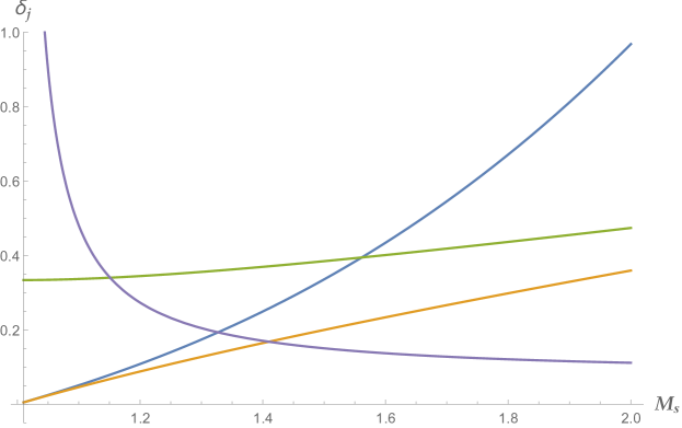
Figure 1: $\delta_{j}$ vs. $M_{\rm s}$, based on Ref. [26, Fig. 2], for the gas Ar. Blue: Case (i). Orange: Case (ii). Green: Case (iii). Lavender: Case (iv).

8.3 Determination of $Q$-metric values

In Table 1, values of $Q$ based on the parameter values given above for Ar are presented. While those for Cases (ii)–(iv), as well as the $M_{\rm s}=\sqrt{2}$ case of Case (i) (see Appendix B), were computed using expressions obtained from evaluating the integrals in Eq. (36) analytically, the entries corresponding to the remaining $M_{\rm s}$ values under Case (i) were computed from the numerical solution of Eq. (39), the process of which involved use of both the NDSolve[  ] and NIntegrate[  ] commands provided in Mathematica.

Table 1: Values of $Q$ in Ar corresponding to Cases (i)–(iv) for selected Mach number values

[t] Case $\underset{(\textrm{Ma}=0.01)}{M_{\rm s}\approx 1.005}$ $\underset{(\textrm{Ma}=1/\sqrt{2})}{M_{\rm s}=\sqrt{2}}$ $\underset{(\textrm{Ma}=2/\sqrt{3})}{M_{\rm s}=\sqrt{3}}$ $\underset{(\textrm{Ma}=3/2)}{M_{\rm s}=2}$ (i) 1.010 2 3.000 4.000 (ii) 1.015 2.710 4.819 7.213 (iii)^† 1.014 2.585 4.464 6.535 (iv)^‡ 2.625 6.885 12.239 18.378

• For this case, $\mp\infty$ in Eq. (36) have been changed to $\mp\tfrac{1}{4}\pi\ell_{\rm iii}$, respectively.

• For this case, $+\infty$ in Eq. (36) has been changed to $\ell_{\rm iv}\ln(2)$.

From Table 1 it is clear that, in all cases shown, $Q$ is a strictly increasing function of the shock Mach number; i.e., profile asymmetry increases with $M_{\rm s}$. This behavior, we observe, is in agreement with the data presented in Refs. [19, 26] for non-isothermal shock propagation in Ar. It is also clear from Table 1 that Cases (i)–(iii) all yield values of $Q$ that are quite close to unity (i.e., quite close to being perfectly symmetric), and to each other, for $\textrm{Ma}=0.01$. In this regard, we point out that $\textrm{Ma}\ll 1$ defines the “realm” of finite-amplitude (or weakly-nonlinear) acoustics theory, within which velocity traveling wave profiles can be expected to have the form of Eqs. (54) and (56); see, e.g., Refs. [25, 27], as well as those cited therein.

Finally, the last three entries in the first row of Table 1 highlight the following noteworthy feature associated with Case (i):

$$\int_{-\infty}^{0}[1-R(\zeta)]\,\textrm{d}\zeta=M_{\rm s}^{2}\int_{0}^{+\infty}R(\zeta)\,\textrm{d}\zeta,$$ (84)

for $M_{\rm s}=\sqrt{2},\sqrt{3},2$. Interestingly, as shown in Appendix B, these values are three of the five shock Mach number values for which Case (i) yields explicit TWSs.

8.4 Determination of $\textrm{Ma}_{\rm sup}$ values

Implicit in Eq. (30b) is the thermodynamic requirement $\Theta_{\rm e}>0$. A simplified approach—which usually yields only approximate results, however—of ensuring that this inequality is everywhere satisfied begins with recasting Eq. (30b) as the inequality

$$0<c_{\rm v}\varkappa_{0}\vartheta_{0}-b_{0}^{2}\max|f^{\prime}|-(4/3)\max\left[\frac{\mu(v-f)\left|f^{\prime}\right|^{2}}{\rho_{0}v}\right]\!,$$ (85)

which is easily broken down into the individual cases

$$0<c_{\rm v}\varkappa_{0}\vartheta_{0}-\begin{cases}\displaystyle{\frac{b_{0}^{2}u_{\rm p}}{\ell_{\rm i}}+\frac{4\nu_{0}}{3}\!\left(\frac{u_{\rm p}^{2}}{\ell_{\rm i}^{2}}\right)},&\text{(i)},\\ \displaystyle{\frac{b_{0}^{2}u_{\rm p}}{\ell_{\rm ii}}+\frac{4\nu_{0}}{3}\!\left(\frac{u_{\rm p}^{2}}{\ell_{\rm ii}^{2}}\right)},&\text{(ii)},\end{cases}$$ (86)

$$0<c_{\rm v}\varkappa_{0}\vartheta_{0}-\begin{cases}\begin{cases}\displaystyle{\frac{b_{0}^{2}u_{\rm p}}{\ell_{\rm iii}}+\frac{9\lambda_{0}^{2}}{4}\!\left(\frac{u_{\rm p}^{3}}{\ell_{\rm iii}^{3}}\right)},&|\zeta|\in[0,\tfrac{\pi}{4}\ell_{\rm iii}),\\ 0,&|\zeta|\geq\tfrac{\pi}{4}\ell_{\rm iii},\end{cases}&\text{(iii)},\\ \\ \begin{cases}\displaystyle{\frac{b_{0}^{2}u_{\rm p}}{\ell_{\rm iv}}+3\lambda_{0}\!\left(\frac{u_{\rm p}^{3}}{\ell_{\rm iv}^{2}}\right)},&\zeta<\ell_{\rm iv}\ln(2),\\ 0,&\zeta\geq\ell_{\rm iv}\ln(2),\end{cases}&\text{(iv)},\end{cases}$$ (87)

where, in deriving these inequalities, we have made use of Eq. (32). It is noteworthy that, because $f$ is a semi-compact function under our two artificial viscosity laws, both inequalities in Relation (87) become simply $0<\vartheta_{0}$ on those intervals of the $\zeta$-axis over which $f$ (and therefore $f^{\prime}$) is identically zero.

In the remainder of this subsection, we seek the value of $\textrm{Ma}_{\rm sup}$ for each case appearing in Relations (86) and (87), assuming one exists, where $\textrm{Ma}\geq\textrm{Ma}_{\rm sup}$ means that isothermal propagation is not possible because the speed of the piston (i.e., $u_{\rm p}$) is too great relative to $b_{0}$. The numerical values given below were computed based on $\gamma=5/3$ and the simplifying assumption $M_{\rm r}=1$, where we define the radiative Mach number as $M_{\rm r}:=b_{0}^{-1}\sqrt{\varkappa_{0}\nu_{0}}$.

8.4.1 Case (i)

In dimensionless form, this case of Relation  (86) can be recast as $0<\Pi_{\rm i}(\textrm{Ma})$, where

$$\Pi_{\rm i}(\textrm{Ma})=\Omega_{\rm i}(M_{\rm r})-\left(\textrm{Ma}+\sqrt{4+\textrm{Ma}^{2}}\,\right)\!\left(-2+\sqrt{4+\textrm{Ma}^{2}}\,\right)\\ -\tfrac{1}{2}\left[\left(\textrm{Ma}+\sqrt{4+\textrm{Ma}^{2}}\,\right)\!\left(-2+\sqrt{4+\textrm{Ma}^{2}}\,\right)\right]^{2},$$ (88)

and where we have set $\Omega_{\rm i}(M_{\rm r})=(8/3)M_{\rm r}^{2}/(\gamma-1)$.

On solving $\Pi_{\rm i}(\textrm{Ma}_{\rm sup}^{0})=0$, which is readily accomplished due to its bi-quadratic form, we find that $\textrm{Ma}_{\rm sup}\approx\textrm{Ma}_{\rm sup}^{0}$, where

$$\textrm{Ma}_{\rm sup}^{0}=\begin{cases}\frac{2Y_{\rm i}-\sqrt{2Y_{\rm i}}|Y_{\rm i}-4|}{2(Y_{\rm i}-2)},&\Omega_{\rm i}(M_{\rm r})\neq 4,\\ 3/2,&\Omega_{\rm i}(M_{\rm r})=4;\end{cases}$$ (89)

here, $Y_{\rm i}=-1+\sqrt{1+2\Omega_{\rm i}(M_{\rm r})}$, where we observe that $\Omega_{\rm i}(M_{\rm r})=4$ yields $Y_{\rm i}=2$, and we have introduced the “dummy” variable $\textrm{Ma}_{\rm sup}^{0}$.

Unfortunately, $\textrm{Ma}_{\rm sup}^{0}$ is not, generally speaking, a very accurate approximation to $\textrm{Ma}_{\rm sup}$ under this case. This is due to the fact that, in general,

$$\max\big{|}\Theta_{\rm e}(\zeta)\big{|}>\big{|}\Theta_{\rm e}(\zeta_{\rm i}^{\bullet})\big{|},$$ (90)

i.e., $\zeta_{\rm i}^{\rm e}\neq\zeta_{\rm i}^{\bullet}$, where $\Theta_{\rm e}^{\prime}(\zeta_{\rm i}^{\rm e})=0$. One can, in principle, determine $\textrm{Ma}_{\rm sup}$ for this case exactly by setting $\Theta_{\rm e}^{\prime}(\zeta)=0$, after first using Eq. (39) to eliminate $f^{\prime}$ from Eq. (30b) and then applying $\textrm{d}/\textrm{d}\zeta$ to the result. The need to employ Ferrari’s technique to solve the resulting quartic, however, renders this approach far too involved, algebraically speaking, to be performed here. Instead, we turn once again to Mathematica’s NDSolve[] command to numerically evaluate Eq. (30b) in order to determine bounds on the value of $\textrm{Ma}_{\rm sup}$.

Omitting the details, it is not difficult to show that under Case (i):

$$\textrm{Ma}_{\rm sup}^{0}=3/2<1.64108<\textrm{Ma}_{\rm sup}<1.64109\qquad(M_{\rm r}=1,\gamma=5/3),$$ (91)

where it should be noted that setting $\textrm{Ma}_{\rm sup}=1.64109$ yields $\min[\Theta_{\rm e}(\zeta)]<0$.

8.4.2 Case (ii)

When expressed in dimensionless form, after using Eq. (57) to eliminate $\ell_{\rm ii}$, this case of Eq. (86) becomes $0<\Pi_{\rm ii}(\textrm{Ma})$, where

$$\Pi_{\rm ii}(\textrm{Ma})=\Omega_{\rm ii}(M_{\rm r})-\textrm{Ma}^{2}-\tfrac{1}{4}\textrm{Ma}^{4},$$ (92)

and where $\Omega_{\rm ii}(M_{\rm r})=2\Omega_{\rm i}(M_{\rm r})=(16/3)M_{\rm r}^{2}/(\gamma-1)$.

Because $\Theta_{\rm e}^{\prime}(\zeta_{\rm ii}^{\bullet})=0$ for all $\textrm{Ma}>0$, where recall that $\zeta_{\rm ii}^{\bullet}=0$, solving $\Pi_{\rm ii}(\textrm{Ma}_{\rm sup})=0$ will give us the exact value of $\textrm{Ma}_{\rm sup}$ for this case; recall Footnote 7. Since $\Pi_{\rm ii}(\textrm{Ma}_{\rm sup})$ is a bi-quadratic, it is easily established that the only positive root $\Pi_{\rm ii}(\textrm{Ma}_{\rm sup})=0$ is

$$\textrm{Ma}_{\rm sup}=\sqrt{-2+2\sqrt{1+\Omega_{\rm ii}(M_{\rm r})}}.$$ (93)

Thus, under Case (ii):

$$\textrm{Ma}_{\rm sup}=2\qquad(M_{\rm r}=1,\gamma=5/3).$$ (94)

8.4.3 Case (iii)

In dimensionless form, this case of Eq. (86) can be recast as $0<\Pi_{\rm iii}(\textrm{Ma})$; here,

$$\Pi_{\rm iii}(\textrm{Ma})=\Omega_{\rm iii}(M_{\rm r})-\tfrac{1}{3}\textrm{Ma}-\tfrac{1}{12}\textrm{Ma}^{3},$$ (95)

where the $\mathfrak{b}_{\rm iii}=\tfrac{1}{4}\sqrt{27}$ special case of Eq. (65) has been used to eliminate $\ell_{\rm ii}$. Also, we have set

$$\Omega_{\rm iii}(M_{\rm r})=\frac{16M_{\rm r}^{2}}{(\gamma-1)\sqrt{50\pi}},$$ (96)

from which we have eliminated $\lambda_{0}$ with the aid of Eq. (21).

Because $\Theta_{\rm e}^{\prime}(\zeta_{\rm iii}^{\bullet})=0$ for all $\textrm{Ma}>0$, where recall that $\zeta_{\rm iii}^{\bullet}=0$, solving $\Pi_{\rm iii}(\textrm{Ma}_{\rm sup})=0$ will give us the exact value of $\textrm{Ma}_{\rm sup}$ for this case; recall, again, Footnote 7. Since $\Pi_{\rm iii}(\textrm{Ma}_{\rm sup})$ is a depressed cubic, applying Cardano’s formula is a relatively simple matter; omitting the details, we find that

$$\textrm{Ma}_{\rm sup}=\sqrt[3]{6\Omega_{\rm iii}(M_{\rm r})+2\sqrt{9\Omega_{\rm iii}^{2}(M_{\rm r})+\tfrac{16}{27}}}\\ +\sqrt[3]{6\Omega_{\rm iii}(M_{\rm r})-2\sqrt{9\Omega_{\rm iii}^{2}(M_{\rm r})+\tfrac{16}{27}}},$$ (97)

which is the only positive root of $\Pi_{\rm iii}(\textrm{Ma}_{\rm sup})=0$.

Thus, under Case (iii):

$$\textrm{Ma}_{\rm sup}\approx 2.379\qquad(M_{\rm r}=1,\gamma=5/3).$$ (98)

Remark 5: The $\Theta_{\rm e}^{\prime}(\zeta)$ vs. $\zeta$ profile exhibits two jumps under Case (iii), the amplitudes and locations of which are:

$$[\![\Theta_{\rm e}^{\prime}\,]\!]\Big{|}_{-\tfrac{\pi}{4}\ell_{\rm iii}}=[\![\Theta_{\rm e}^{\prime}\,]\!]\Big{|}_{+\tfrac{\pi}{4}\ell_{\rm iii}}=\frac{2b_{0}^{2}u_{\rm p}}{9c_{\rm v}\varkappa_{0}\lambda_{0}^{2}}.$$ (99)

8.4.4 Case (iv)

Because the Case (iv) version of Eq. (30b) exhibits explicit dependence on not only $f^{\prime}$ but also $f$, the corresponding case of Eq. (87) will only yield an approximation to $\textrm{Ma}_{\rm sup}$—one that can be shown to be quite poor.

Hence, let us specialize Eq. (30b) to Case (iv) (see Section 7), with $\mathfrak{b}_{\rm iv}=9/2$, and then replace $\Theta_{\rm e}(\zeta)$ with its dimensionless counterpart $T_{\rm e}(\zeta)$; doing so yields, after simplifying, the exact expression

$$T_{\rm e}(\zeta)=\Omega_{\rm iv}(M_{\rm r})-\begin{cases}\tfrac{1}{6}\textrm{Ma}\exp(\zeta/\ell_{\rm iv})\\ \qquad+\tfrac{1}{12}\textrm{Ma}^{3}\exp(2\zeta/\ell_{\rm iv})\\ \qquad\qquad-\tfrac{1}{24}\textrm{Ma}^{3}\exp(3\zeta/\ell_{\rm iv})&\zeta<\zeta_{\rm iv}^{\bullet},\\ 0,&\zeta\geq\zeta_{\rm iv}^{\bullet},\end{cases}$$ (100)

where $T_{\rm e}(\zeta)\propto\Theta_{\rm e}(\zeta)$ and $\Omega_{\rm iv}(M_{\rm r})=\Omega_{\rm iii}(M_{\rm r})$.

Although doing so is not simply a matter of setting $T_{\rm e}^{\prime}(\zeta)=0$, it can be shown that $\zeta_{\rm iv}^{\rm e}$, the critical point of $T_{\rm e}(\zeta)$ under this case, is exactly given by

$$\zeta_{\rm iv}^{\rm e}=\begin{cases}\ell_{\rm iv}\ln[Y_{\rm iv}(\textrm{Ma})],&\textrm{Ma}>1,\\ \zeta_{\rm iv}^{\bullet}=\ell_{\rm iv}\ln(2),&\textrm{Ma}\leq 1,\end{cases}$$ (101)

where we have set

$$Y_{\rm iv}(\textrm{Ma})=\frac{2\textrm{Ma}+2\sqrt{3+\textrm{Ma}^{2}}}{3\textrm{Ma}}\qquad(\textrm{Ma}>1).$$ (102)

Here, we observe that $T_{\rm e}^{\prime}(\zeta_{\rm iv}^{\rm e})=0$ only for $\textrm{Ma}>1$, where the corresponding stationary point of the $T_{\rm e}(\zeta)$ vs. $\zeta$ profile is also its absolute minimum; for $\textrm{Ma}\leq 1$, in contrast, $\inf[T_{\rm e}(\zeta)]=\lim_{\zeta\to(\zeta_{\rm iv}^{\bullet})^{-}}T_{\rm e}(\zeta)$.

Consequently, we are led to consider the inequality $0<\Pi_{\rm iv}(\textrm{Ma})$, where

$$\Pi_{\rm iv}(\textrm{Ma})=\Omega_{\rm iv}(M_{\rm r})-\begin{cases}\tfrac{1}{6}\textrm{Ma}Y_{\rm iv}+\tfrac{1}{12}\textrm{Ma}^{3}Y_{\rm iv}^{2}-\tfrac{1}{24}\textrm{Ma}^{3}Y_{\rm iv}^{3},&\textrm{Ma}>1,\\ \tfrac{1}{3}\textrm{Ma},&\textrm{Ma}\leq 1.\end{cases}$$ (103)

Eq. (103) follows from Eq. (100) on setting $\Pi_{\rm iv}(\textrm{Ma})=T_{\rm e}(\zeta_{\rm iv}^{\rm e})$, and as such contains no approximations.

It is now possible to determine $\textrm{Ma}_{\rm sup}$ exactly by solving $\Pi_{\rm iv}(\textrm{Ma}_{\rm sup})=0$, which can be simplified to read

$$0=\begin{cases}(243\Omega_{\rm iv}^{2}(M_{\rm r})-4)-54\Omega_{\rm iv}(M_{\rm r})\textrm{Ma}_{\rm sup}\\ \qquad-\textrm{Ma}_{\rm sup}^{2}-12\Omega_{\rm iv}(M_{\rm r})\textrm{Ma}_{\rm sup}^{3},&M_{\rm r}>M_{\rm r}^{\star},\\ \Omega_{\rm iv}(M_{\rm r})-\tfrac{1}{3}\textrm{Ma}_{\rm sup},&M_{\rm r}\leq M_{\rm r}^{\star},\end{cases}$$ (104)

where we note the critical value

$$M_{\rm r}^{\star}:=\frac{1}{2}\sqrt{\frac{5(\gamma-1)}{3}\sqrt{\frac{\pi}{8}}},$$ (105)

and we observe that $\Omega_{\rm iv}(M_{\rm r}^{\star})=1/3$.

While it is a trivial matter to establish that

$$\textrm{Ma}_{\rm sup}=3\Omega_{\rm iv}(M_{\rm r})\qquad(M_{\rm r}\leq M_{\rm r}^{\star}),$$ (106)

suffice it to say that the process of determining $\textrm{Ma}_{\rm sup}$ for the cubic case of Eq. (104) is algebraically intensive. As such, we set our analytical efforts aside and return to our numerical tools; hence, following an approach similar to that used in Section 8.4.1, we find that under Case (iv):

$$2.92641<\textrm{Ma}_{\rm sup}<2.92642\quad(M_{\rm r}=1,\gamma=5/3),$$ (107)

where we note that setting $\textrm{Ma}_{\rm sup}=2.92642$ yields
$\min[T_{\rm e}(\zeta)]<0$. And to help clarify the nature of the absolute minimum it exhibits, we have plotted $T_{\rm e}(\zeta)$ vs. $\zeta$ in Fig. 2(a,b), where the plots in the former and latter correspond to $M_{\rm r}>M_{\rm r}^{\star}$ and $M_{\rm r}\leq M_{\rm r}^{\star}$, respectively. Remark 6: The temperature of the surrounding environment must exhibit a jump discontinuity across $\zeta=\zeta_{\rm iv}^{\bullet}$ under the present case; specifically (recall Eq. (38))

$$[\![T_{\rm e}]\!]\big{|}_{\zeta_{\rm iv}^{\bullet}}=(\Omega_{\rm iv}(M_{\rm r})-\tfrac{1}{3}\textrm{Ma})-\Omega_{\rm iv}(M_{\rm r})=-\tfrac{1}{3}\textrm{Ma},$$ (108)

for all $\textrm{Ma}>0$. The plots in Fig. 2(a,b) also serve to illustrate this phenomenon, with $\textrm{Ma}_{\rm sup}$ in the role of Ma. Evaluating numerically, we find that $[\![T_{\rm e}]\!]\big{|}_{\zeta_{\rm iv}^{\bullet}}\approx-0.9755$ and $[\![T_{\rm e}]\!]\big{|}_{\zeta_{\rm iv}^{\bullet}}\approx-0.0833$, respectively, in Fig. 2(a,b).

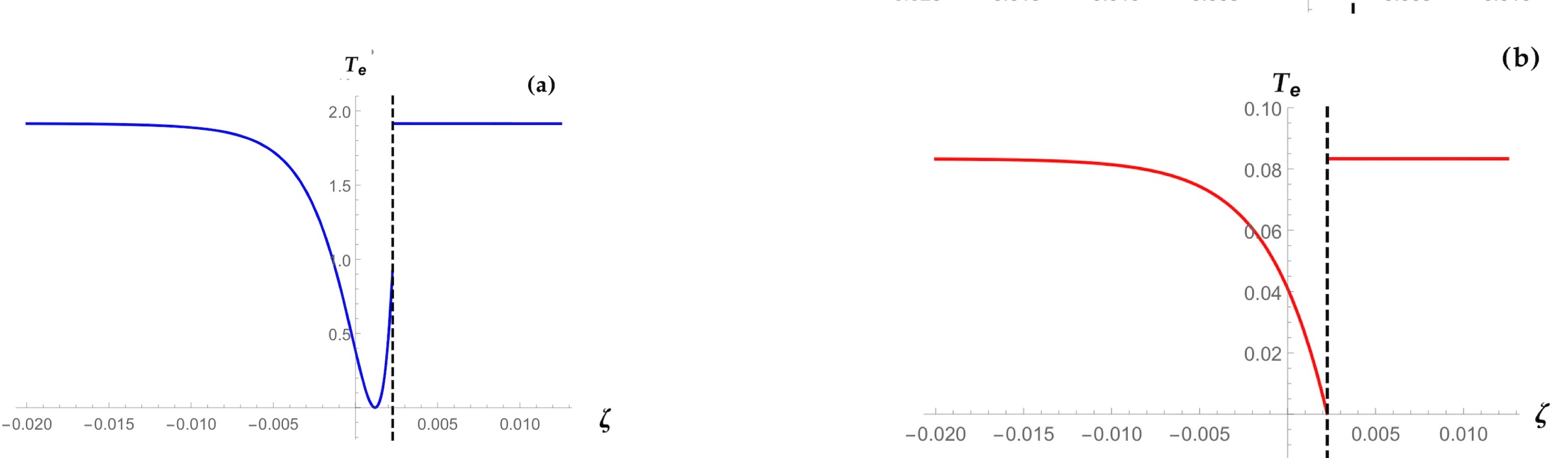
Figure 2: $T_{\rm e}(\zeta)$ vs. $\zeta$ generated from Eq. (100) using the parameter values for Ar given in Section 8.1, where we recall that $\mathfrak{b}_{\rm iv}=9/2\implies\ell_{\rm iv}=3\lambda_{0}$; here, $M_{\rm r}^{\star}\approx 0.4172$. Blue curve: $M_{\rm r}=1$ (see Eq. (107)). Red curve: $M_{\rm r}=\tfrac{1}{2}M_{\rm r}^{\star}$ ($\implies\textrm{Ma}_{\rm sup}=1/4$). Black-broken line: $\zeta=\zeta_{\rm iv}^{\bullet}=3\lambda_{0}\ln(2)\approx 0.0023$.

9 Closing remarks and observations

1. If $\textrm{Ma}=1$, then $v=b_{0}\varphi$, where $\varphi\approx 1.618$ is the proportio divina [29]; in other words, if $u_{\rm p}=b_{0}$, then

   $$v\approx b_{0}\left(\frac{F_{N+1}}{F_{N}}\right)\qquad(N\gg 1),$$ (109)

   where $F_{N}$ denotes the $N$th Fibonacci number; see Ref. [29, p. 101]. (Note that $F_{1}=F_{2}=1$.)

2. While $f,g\in\mathcal{C}^{\infty}(\mathbb{R})$ under both Cases (i) and (ii), the same is not true under Cases (iii) and (iv); specifically, $f,g\in\mathcal{C}^{1}(\mathbb{R})$ and $f,g\in\mathcal{C}^{0}(\mathbb{R})$, respectively, under the former and latter.

3. By averaging the (1D) Euler system under finite-scale theory (FST), one obtains a system containing an “effective viscosity” that is given by Eq. (17) with $\mathfrak{b}_{\rm iii}=1/\sqrt{12}$ and $\lambda_{0}$ replaced by $L$, where $L(>0)$ is the length scale that appears in the averaging transform of FST; see Refs. [13, 30] and those cited therein.

4. The $\Theta_{\rm e}(\zeta)$ vs. $\zeta$ profile under Case (iii) admits a pair of temperature-rate waves (see, e.g., Refs. [20, 31, 32]), i.e., jumps in $\Theta_{\rm e}^{\prime}(\zeta)$; see Remark 5.

5. A thermal shock (see, e.g., Refs. [31, 32]), i.e., a jump in $T_{\rm e}(\zeta)$, must occur under Case (iv); see Remark 6.

6. While they are quite distinct from those presented for Ar in Refs. [19, 26], the TWS profiles generated under Case (iv) are very similar to those given in Ref. [33, Fig. 2], which depict non-isothermal shocks in CO₂; see also Ref. [34].

Acknowledgments

All numerical computations and simulations presented above were performed using Mathematica, ver. 11.2. S.C.  wishes to acknowledge the financial support of GNFM-INdAM, INFN, and Sapienza University of Rome, Italy. P.M.J.  was supported by U.S. Office of Naval Research (ONR) funding.

Appendix A Appendix: Comparison with Stokes (1851)

In this appendix the EoM derived by Stokes in Ref. [2], which describes non-isothermal propagation with radiation under the linear approximation, is re-derived. We also give the isothermal version of Stokes’ model and the linearized, reduced, version of the present (i.e., isothermal) governing system. Key aspects of all three models are noted and briefly discussed.

In terms of the present notation, the governing system of equations considered by Stokes [2], and later Rayleigh [10, § 247], can be expressed as

$$s_{t} =-u_{x},$$ (A.1a)

$$\rho_{0}u_{t} =-p_{x}$$ (A.1b)

$$\theta_{t}-(\gamma-1)s_{t} =-\varkappa_{0}\theta,$$ (A.1c)

$$p =p_{0}(1+s+\theta).$$ (A.1d)

In Sys. (A.1), $s=(\rho-\rho_{0})/\rho_{0}$ is known as the condensation; we have set $\theta=(\vartheta-\vartheta_{0})/\vartheta_{0}$; the term on the right-hand side of Eq. (A.1c) follows from taking, prior to cancellation of the product $c_{\rm v}\rho_{0}\vartheta_{0}$,

$$r=-c_{\rm v}\varkappa_{0}\vartheta_{0}\theta,$$ (A.2)

i.e., $r$ to be given by the general (i.e., non-isothermal) form of Newton’s law of cooling; and $\mu$, $\mu_{\rm b}$, and $K$ have all been set equal to zero. (Unless stated herein, the definitions of all quantities, terms, etc., appearing in this appendix can be found in Section 2.)

Now using Eqs. (A.1a) and (A.1d) to eliminate $u$ and $p$, respectively, from Eq. (A.1b) reduces Sys. (A.1) to

$$s_{tt} =b_{0}^{2}s_{xx}+b_{0}^{2}\theta_{xx},$$ (A.3a)

$$(\varkappa_{0}+\partial_{t})\theta =(\gamma-1)s_{t},$$ (A.3b)

where we have re-written Eq. (A.1c) in operator form.

At this point it is instructive to introduce the isothermal counterpart of Sys. (A.3):

$$s_{tt}-b_{0}^{2}s_{xx} =0,$$ (A.4a)

$$\vartheta_{\rm e} =\vartheta_{0}[1-\varkappa_{0}^{-1}(\gamma-1)s_{t}],$$ (A.4b)

where, as in Section 2.3, $\vartheta_{\rm e}=\vartheta_{\rm e}(x,t)$ is controllable by the experimenter, and

$$s_{tt}-b_{0}^{2}s_{xx} =\tfrac{4}{3}\nu_{0}s_{txx},$$ (A.5a)

$$\vartheta_{\rm e} =\vartheta_{0}[1-\varkappa_{0}^{-1}(\gamma-1)s_{t}],$$ (A.5b)

which is easily obtained from the linearized version of Sys. (13). Here, in parallel with the analyses carried out in Section 8.4, we stress the fact that if $s_{t}>0$ (i.e., compression) is a possibility, then suitable additional restrictions must be placed on the boundary and/or initial data for Eqs. (A.4a) and (A.5b) to ensure that Eqs. (A.4b) and (A.5b) yield $\vartheta_{\rm e}>0$.

In closing, we return to Sys. (A.3) and, on eliminating $\theta$ between its two PDEs, obtain the modern form of the EoM first derived by Stokes in 1851, viz.,

$$s_{ttt}-c_{0}^{2}s_{txx}+\varkappa_{0}(s_{tt}-b_{0}^{2}s_{xx})=0;$$ (A.6)

see Refs. [2, Eq. (7)] and [10, § 247(6)]. In recent years, many authors have begun referring to PDEs of this type as (Stokes–)Moore–Gibson–Thompson equations; see, e.g., Ref. [35, p. 3], wherein an interesting stability condition for Eq. (A.6) and its multi-D extensions is presented and discussed.

With regard to modeling experiments involving both radiation and non-isothermal conditions, we observe that Sys. (A.3) is preferred to Eq. (A.6) in terms of initial data requirements. That is, while both formulations require knowledge of $s(x,0)$ and $s_{t}(x,0)$, it appears to be much easier, from the standpoint of performing the experiment, for one to accurately specify (and enforce) $\theta(x,0)$ than $s_{tt}(x,0)$.

Appendix B Appendix: Explicit TWSs under Case (i)

We begin with the observation that Eq. (43) can also be written as

$$\frac{3v\zeta}{2\nu_{0}(|k|-1)}=\ln(1-\mathcal{F})-\left(\frac{|k|+1}{|k|-1}\right)\ln(1+\mathcal{F})\qquad(|\mathcal{F}|<1),$$ (B.1)

where we recall that $k<-1$. Prompted by the special case TWS derived in Ref. [27, § 4], wherein Becker’s assumption (see also Ref. [18]) was adopted, we find that setting $\textrm{Ma}=1/\sqrt{2}$ ($\implies k=-3$, $M_{\rm s}=\sqrt{2}$) reduces Eq. (B.1) to

$$\left(\frac{3b_{0}\sqrt{2}}{4\nu_{0}}\right)\zeta=\ln\left[\frac{1-\mathcal{F}}{(1+\mathcal{F})^{2}}\right]\!,$$ (B.2)

which is readily solved to yield the explicit expression

$$f(\zeta)=\frac{1}{4}u_{\rm p}\exp\left[-(3+2\sqrt{2}\,)\zeta/\ell_{\rm i}\right]\times\left\{-1+\sqrt{1+8\exp\left[(3+2\sqrt{2}\,)\zeta/\ell_{\rm i}\right]}\,\right\}\!,$$ (B.3)

where we recall our use of the relation $\mathcal{F}(\zeta)=-1+(2/u_{\rm p})f(\zeta)$. In the case of Eq. (B.3), the shock thickness and corresponding stationary point are given by

$$\ell_{\rm i}=\frac{\nu_{0}(3+2\sqrt{2})\sqrt{8}}{3b_{0}},\,\,\,\,\zeta_{\rm i}^{\bullet}=\left(\frac{4\nu_{0}}{b_{0}\sqrt{18}}\right)\ln\!\left[\tfrac{1}{4}(1+\sqrt{2}\,)\right]\!,$$ (B.4)

respectively.

The corresponding density TWS is easily found to be

$$g(\zeta)=\!\rho_{0}\Bigg{(}1-\tfrac{1}{8}\exp\left[-(3+2\sqrt{2}\,)\zeta/\ell_{\rm i}\right]\times\left\{-1+\sqrt{1+8\exp\left[(3+2\sqrt{2}\,)\zeta/\ell_{\rm i}\right]}\,\right\}\Bigg{)}^{-1}\!\!\!\!,$$ (B.5)

and its shock thickness and stationary point are given by

$$l_{\rm i}=2(\nu_{0}/b_{0})\sqrt{6},\qquad\zeta_{\rm i}^{*}=-l_{\rm i}\ln\left(2\right)\!.$$ (B.6)

We close by pointing out that four other explicit TWSs are possible under Case (i). Apart from noting that obtaining them requires one to solve the cubic and quartic equations

$$(1-\mathcal{F})\exp\left[-\,\frac{3b_{0}\zeta\sqrt{m}}{2\nu_{0}(|k|-1)}\right]=(1+\mathcal{F})^{m},$$ (B.7)

however, we leave their derivations to the reader; here,

$$m=\begin{cases}4/3(\implies k=-7),&\textrm{Ma}=1/\sqrt{12},\\ 3/2(\implies k=-5),&\textrm{Ma}=1/\sqrt{6},\\ 3(\implies k=-2),&\textrm{Ma}=2/\sqrt{3},\\ 4(\implies k=-5/3),&\textrm{Ma}=3/2,\end{cases}$$ (B.8)

where $m(>1)$ is given by $m=(|k|+1)(|k|-1)^{-1}=M_{\rm s}^{2}$.

References

- [1] Stokes GG (1849) On the theories of the internal friction of fluids in motion, and of the equilibrium and motion of elastic solids. Trans Camb Phil Soc 8(Pt III): 287–319
- [2] Stokes GG (1851) An examination of the possible effect of the radiation of heat on the propagation of sound. Phil Mag (Ser 4) 1(4): 305–317
- [3] Lord Rayleigh (1910) Aerial plane waves of finite amplitude. Proc Roy Soc Lond A 84: 247–284
- [4] Lamb H (1945) Hydrodynamics, 6th edn. Dover Publications, New York
- [5] Truesdell C (1953) Precise theory of the absorption and dispersion of forced plane infinitesimal waves according to the Navier–Stokes equations. J Rational Mech Anal 2: 643–741
- [6] LeVeque RJ (2004) The dynamics of pressureless dust clouds and delta waves. J Hyperbolic Diff Eqs 1(2): 315–327
- [7] Chandrasekhar S (1967) An Introduction to the study of stellar structure, Dover Publications, New York
- [8] Thompson PA (1972) Compressible-fluid dynamics. McGraw–Hill, New York
- [9] Pierce AD (1989) Acoustics: An introduction to its physical principles and applications, Acoustical Society of America, Woodbury, NY
- [10] Lord Rayleigh (1896) Theory of sound, vol II, 2nd edn. MacMillan and Company, London
- [11] Chapman S, Cowling TG (1970) The mathematical theory of non-uniform gases, 3rd edn. Cambridge University Press, Cambridge
- [12] Truesdell C, Muncaster RG (1980) Fundamentals of Maxwell’s kinetic theory of a simple monatomic gas, Academic Press, New York
- [13] Margolin LG, Vaughan DE (2012) Traveling wave solutions for finite scale equations. Mech Res Commun 45: 64–69
- [14] von Neumann J, Richtmyer RD (1950) A method for the numerical calculation of hydrodynamic shocks. J Appl Phys 21: 232–237
- [15] Roache PJ (1972) Computational fluid dynamics. Hermosa Publishers, Albuquerque, NM
- [16] Evans MW, Harlow FH (1957) The particle-in-cell method for hydrodynamic calculations, Los Alamos Scientific Laboratory, Report No. LA-2139. Los Alamos, NM
- [17] Longley HJ (1960) Methods of differencing in Eulerian hydrodynamics, Los Alamos Scientific Laboratory, Report No. LAMS-2379. Los Alamos, NM
- [18] Morduchow M, Libby PA (1949) On a complete solution of the one-dimensional flow equations of a viscous, heat-conducting, compressible gas. J Aeronaut Sci 16: 674–684, and 704
- [19] Schmidt B (1969) Electron beam density measurements in shock waves in argon. J Fluid Mech 39: 361–373
- [20] Morro A (2006) Jump relations and discontinuity waves in conductors with memory. Math Comput Modelling 43: 138–149
- [21] Straughan B (2008) Stability and wave motion in porous media, Applied Mathematical Sciences, vol 165. Springer, Berlin/Heidelberg
- [22] Bland, DR (1988) Wave theory and applications, Oxford University Press, Oxford
- [23] Bissell J, Straughan B (2014) Discontinuity waves as tipping points: applications to biological & sociological systems, Discrete Cont Dyn Sys, Ser B 19: 1911–1934
- [24] Davis HT (1962) Introduction to nonlinear differential and integral equations. Dover Publications, New York
- [25] Christov IC, Jordan, PM, Chin-Bing SA, Warn-Varnas A (2016) Acoustic traveling waves in thermoviscous perfect gases: Kinks, acceleration waves, and shocks under the Taylor–Lighthill balance. Math Comput Simuln 127: 2–18
- [26] Alsmeyer H (1976) Density profiles in argon and nitrogen shock waves measured by the absorption of an electron beam. J Fluid Mech 74: 497–513
- [27] Margolin LG, Reisner JM, Jordan PM (2017) Entropy in self-similar shock profiles. Int J Non-Linear Mech 95: 333–346
- [28] Destrade M, Gaeta G, Saccomandi G (2007) Weierstrass’s criterion and compact solitary waves. Phys Rev E 75: 047601
- [29] Livio M (2002) The golden ratio, Broadway Books, New York
- [30] Margolin LG, Plesko CS, Reisner JM (2020) Finite scale theory: Predicting nature’s shocks. Wave Motion 98: 102647
- [31] Straughan B (2011) Heat waves, Applied Mathematical Sciences, vol. 177. Springer, Berlin/Heidelberg
- [32] Sellitto A, Zampoli V, Jordan PM (2020) Second-sound beyond Maxwell–Cattaneo: Nonlocal effects in hyperbolic heat transfer at the nanoscale. Int J Engng Sci 154: 103328
- [33] Griffith WC, Kenny A (1957) On fully-dispersed shock waves in carbon dioxide. J Fluid Mech 3: 286–288
- [34] Taniguchi S, Arima T, Ruggeri T, Sugiyama M (2018) Shock wave structure in rarefied polyatomic gases with large relaxation time for the dynamic pressure. J Phys: Conf Ser 1035: 012009
- [35] Kaltenbacher B, Nikolić V (2019) On the Jordan–Moore–Gibson–Thompson equation: well-posedness with quadratic gradient nonlinearity and singular limit for vanishing relaxation time. arXiv:1901.02795v3 [math.AP]: 12 Oct 2019