NRCPS-HE-71-2022

April, 2022

Gauge Field Theory Vacuum and Cosmological Inflation

George Savvidy

Institute of Nuclear and Particle Physics, NCSR Demokritos, GR-15310 Athens, Greece
A.I. Alikhanyan National Science Laboratory, Yerevan, 0036, Armenia

The deep interrelation between elementary particle physics and cosmology manifests itself when one considers the contribution of quantum fluctuations of vacuum fields to the dark energy and the effective cosmological constant. The contribution of zero-point energy exceeds by many orders of magnitude the observational cosmological upper bound on the energy density of the universe. Therefore it seems natural to expect that vacuum fluctuations of the fundamental fields would influence the cosmological evolution in any way. Our aim in this review article is to describe a recent investigation of the influence of the Yang-Mills vacuum polarisation and of the chromomagnetic condensation on the evolution of Friedmann cosmology, on inflation and on primordial gravitational waves. We derive the quantum energy-momentum tensor and the corresponding quantum equation of state for gauge field theory using the effective Lagrangian approach. The energy-momentum tensor has a term proportional to the space-time metric and provides a finite non-diverging contribution to the effective cosmological constant. This allows to investigate the influence of the gauge field theory vacuum polarisation on the evolution of Friedmann cosmology, inflation and primordial gravitational waves. The Type I-IV solutions of the Friedmann equations induced by the gauge field theory vacuum polarisation provide an alternative inflationary mechanism and a possibility for late-time acceleration. The Type II solution of the Friedmann equations generates the initial exponential expansion of the universe of finite duration and the Type IV solution demonstrates late-time acceleration. The solutions fulfil the necessary conditions for the amplification of primordial gravitational waves.

1 Introduction

The deep interrelation between elementary particle physics and cosmology manifests itself when one considers the contribution of quantum fluctuations of vacuum fields to the dark energy and cosmological constant $\Lambda_{cc}$ [1, 2, 34, 16, 18, 19, 25, 26, 28]. In discussing the cosmological constant problem, it is assumed that $\Lambda_{cc}$ corresponds to the vacuum energy density, for which there are many contributions and that anything that contributes to the energy density of the vacuum acts as a cosmological constant. The contribution of zero-point energy exceeds by many orders of magnitude the observational cosmological upper bound on the energy density of the universe.

Therefore it seems natural to expect that vacuum fluctuations of the fundamental interactions would influence the cosmological evolution in any way [1, 2]. Our aim in this review article is to describe a recent investigation [3] of the influence of the Yang-Mills vacuum polarisation and of the chromomagnetic condensation [4, 5, 6, 7, 8, 9] on the evolution of Friedmann cosmology [10, 11], on inflation [12, 13, 14, 15, 16, 18, 19, 20, 24, 25, 26] and on primordial gravitational waves [27, 28, 29, 30, 31, 32].

The calculation of the effective Lagrangian in QED by Heisenberg and Euler was the first example of a well-defined physically motivated prescription allowing to obtain a finite, gauge and renormalisation group-invariant result when investigating the vacuum fluctuations of quantised fields [40]. It appears that only the difference between vacuum energy in the presence and in the absence of external sources has a well-defined physical meaning [40, 41, 42, 43, 44, 45, 46, 47, 4, 5, 6, 7, 8]. In [3] we follow this prescription with the aim to derive the quantum equation of state for non-Abelian gauge fields by using the effective Lagrangian approach [48, 49, 50, 51, 52, 53, 54, 55, 56, 57, 58, 59, 60, 61, 62, 63, 64, 65, 66, 67, 68, 69] and analyse the properties of Friedmann cosmology driven by the quantum Yang-Mills equation of state.

In Section 2 we will derive the quantum equation of state (18) for the non-Abelian gauge fields by using the effective Lagrangian approach, and in Section 3 we will analyse the properties of Friedmann cosmology driven by the quantum Yang-Mills equation of state (42) and (44). In the subsequent four sections we will demonstrate that the nonsingular Type II solution of the Friedmann equations (86), (87) provides an alternative mechanism for a very early stage inflation of a finite duration (95), (94) and that there is no initial singularity (84). The Type IV solution provides an early-time expansion of the universe that follows a prolongated phase where the universe remains almost static and subsequently induces a late-time acceleration of a finite duration (122). The Type I solution represents the universe that recollapses in a finite time. The parameters of Type III solution are such that the universe asymptotically approaches a static universe. Infinitesimal deviation of the Type III parameters will place it ether into the Type II or Type IV solutions. In Sections 8 and 9 we consider the solutions of the Friedmann equations in the cases of flat $k=0$ and positive curvature $k=1$ geometries that appear to represent the evolution of the universe of a finite duration. In the last Section 10 we discuss the generation of primordial gravitational waves.

2 Inflation Drive by Scalar Fields

Let us first review in short the basic properties of Friedmann equations and the standard contributions to the energy density and pressure by dust, radiation and barotropic fluid [28, 16, 18, 25, 26]. The equation of state of matter in the universe defines the cosmological evolution and enters on the right-hand side of the first and of the second Friedmann equations [10, 11]:

$${k\over a^{2}}+{\dot{a}^{2}\over a^{2}}={8\pi G\over 3c^{4}}\epsilon,~{}~{}~{}~{}~{}~{}~{}{k\over a^{2}}+{\dot{a}^{2}\over a^{2}}+2{\ddot{a}\over a}=-{8\pi G\over c^{4}}p,$$ (1)

where $\epsilon$ is the energy density, $p$ is a pressure, $\dot{a}={da/cdt}$ and $k$ defines the sign of the curvature. The scale factor $a(t)$ enters into the metric as [28, 16, 18, 25]

$$ds^{2}=c^{2}dt^{2}-a^{2}(t)\begin{cases}d\chi^{2}+\chi^{2}d\Omega^{2}~{}~{}~{}~{}~{}~{}~{}~{}&k=0\\ d\chi^{2}+\sin^{2}\chi d\Omega^{2}~{}~{}~{}~{}~{}~{}~{}~{}~{}&k=1\\ d\chi^{2}+\sinh^{2}\chi d\Omega^{2}~{}~{}~{}~{}~{}~{}~{}~{}~{}~{}~{}~{}~{}~{}&k=-1\end{cases}.$$ (2)

These are comoving coordinates; the universe expands or contracts as $a(t)$ increases or decreases, and the matter coordinates remain fixed. The conformal time $\eta$ is defined as $cdt=a(\eta)d\eta$. It is convenient to transform the Friedmann equations (1) into the following form [28, 16, 25]:

$$\dot{\epsilon}+3{\dot{a}\over a}(\epsilon+p)=0,$$ (3)

$${\ddot{a}\over a}=-{4\pi G\over 3c^{4}}(\epsilon+3p).$$ (4)

The behaviour of the solutions of the Friedmann equations are defined by the equation of state of the matter that filled the universe $p=p(\epsilon)$. In the case of dust of zero pressure $p=0$ it follows from (3) that $\epsilon\ a^{3}=const$ and in the case of pure radiation $p=\epsilon/3$ that $\epsilon\ a^{4}=const.$ The acceleration ${\ddot{a}/a}$ is negative in both these cases $(\epsilon+3p>0)$ and the inflation of the universe is impossible with these equations of state.

Considering the general parametrisation of the equation of state $p=w\epsilon$ in terms of the barotropic parameter $w$ one can find that the solution of (3) has the following form:

$$~{}~{}~{}\epsilon\ a^{3(1+w)}=const$$ (5)

and that in the important case of positive energy density and negative pressure $p=-\epsilon<0$, that is for $w=-1$, one can find that the acceleration in (4) is positive because $\epsilon+3p=-2\epsilon<0$ and we have

$${\ddot{a}\over a}={8\pi G\over 3c^{4}}\epsilon>0,~{}~{}~{}~{}~{}~{}~{}~{}~{}~{}~{}p=-\epsilon<0.$$ (6)

Thus representation the dark energy as a fluid of positive energy density but negative pressure provides a sufficient condition for the accelerating expansion - inflation - of the universe [13, 14, 15, 33, 16, 18, 25, 26]. The inflation became possible because the strong energy dominance condition $\epsilon+3p\geq 0$ is violation by a large negative pressure.

The question is if there exits any field theoretical model that can realise equation of state with negative pressure (6). It has been found that this type of inflation can be driven by a scalar field [16, 18, 20, 21, 22, 23]. A negative pressure fluid is realised because in scalar field theory the energy density and pressure have the following form:

$$\epsilon={1\over 2}\dot{\phi}^{2}+V(\phi),~{}~{}~{}~{}~{}~{}p={1\over 2}\dot{\phi}^{2}-V(\phi)$$ (7)

and therefore $\epsilon+p=\dot{\phi}^{2}\geq 0,~{}\epsilon+3p=2\dot{\phi}^{2}-2V(\phi).$ The inflationary condition $\epsilon+3p<0$ in (4), (6) can be satisfied when the scalar field is in its vacuum state:

$$\dot{\phi}_{0}=0,~{}~{}~{}~{}~{}~{}~{}V^{{}^{\prime}}(\phi_{0})=0,~{}~{}~{}~{}~{}V(\phi_{0})>0,~{}~{}~{}~{}~{}p=-\epsilon<0$$ (8)

and

$$\epsilon+3p=-2V(\phi_{0})<0.$$ (9)

In that case the equation (4) takes the following form

$${\ddot{a}\over a}={8\pi G\over 3c^{4}}V(\phi_{0})>0$$ (10)

and describes a positive acceleration of the universe. It is interesting to know how unique is a scalar field induced inflation and if there exits any other field theoretical model that realises equation of state that allows accelerating expansion (6) of the universe. Our aim is to demonstrate that a similar acceleration condition are realised in the universe that is filled by the gauge field theory vacuum fluctuations [3].

3 Equation of State Describing Gauge Field Theory Vacuum Fluctuations

We will assume here that the universe is filled by the gauge field theory vacuum fluctuations and will analyse the influence of these vacuum fluctuations on the evolution of the universe. At this stage we will neglect the contributions to the energy density from radiation, elementary particles of the Standard Model or of the Grand Unified Theory (GUT). These contributions can be analysed afterwards.

In order to derive the equation of state describing the gauge field theory vacuum fluctuations we will use the explicit expression for the effective Lagrangian [4, 5, 6, 7, 8]. The effective Lagrangian is a sum of the Heisenberg-Euler Lagrangian ${\cal L}_{q}$ [40] taken in the limit of massless chiral fermions [5]:

$${\cal L}_{q} = -{\cal F}+{N_{f}\over 48\pi^{2}}g^{2}{\cal F}\Big{[}\ln({2g^{2}{\cal F}\over\mu^{4}})-1\Big{]}~{},~{}$$ (11)

where $N_{f}$ is the number of fermion flavours and of the Yang-Mills effective Lagrangian ${\cal L}_{g}$ for SU(N) gauge field theory [4, 5, 6]:

$${\cal L}_{g}=-{\cal F}-{11N\over 96\pi^{2}}g^{2}{\cal F}\Big{(}\ln{2g^{2}{\cal F}\over\mu^{4}}-1\Big{)}~{},~{}~{}~{}~{}~{}~{}~{}~{}~{}~{}~{}{\cal G}=G^{*}_{\mu\nu}G^{\mu\nu}=0~{},$$ (12)

where invariant ${\cal F}={1\over 4}g^{\alpha\beta}g^{\gamma\delta}G^{a}_{\alpha\gamma}G_{\beta\delta}\geq 0$ is of a chromomagnetic type. The effective Lagrangian has exact logarithmic dependence on the invariant ${\cal F}$ and we can obtain the quantum energy momentum tensor $T_{\mu\nu}$ by using the expressions (11) and (12) [5]:

$$T_{\mu\nu}=T^{YM}_{\mu\nu}\Big{[}1+{b\ g^{2}\over 96\pi^{2}}\ln{2g^{2}{\cal F}\over\mu^{4}}\Big{]}-g_{\mu\nu}{b\ g^{2}\over 96\pi^{2}}{\cal F},~{}~{}~{}~{}~{}~{}~{}~{}~{}{\cal G}=0,$$ (13)

where $b=11N-2N_{f}$. The vacuum energy density has therefore the following form:

$$T_{00}\equiv\epsilon({\cal F})=~{}{\cal F}+{b\ g^{2}\over 96\pi^{2}}{\cal F}\Big{(}\ln{2g^{2}{\cal F}\over\mu^{4}}-1\Big{)}$$ (14)

and the spacial components of the stress tensor are:

$$T_{ij}=\delta_{ij}~{}\Big{[}{1\over 3}{\cal F}+{1\over 3}{b\ g^{2}\over 96\pi^{2}}{\cal F}\Big{(}\ln{2g^{2}{\cal F}\over\mu^{4}}+3\Big{)}\Big{]}=\delta_{ij}~{}p({\cal F}).$$ (15)

Thus the gauge field theory vacuum fluctuations are described by the following equation of state:

$$\epsilon({\cal F})=~{}{\cal F}+{b\ g^{2}\over 96\pi^{2}}{\cal F}\Big{(}\ln{2g^{2}{\cal F}\over\mu^{4}}-1\Big{)},~{}~{}~{}~{}~{}~{}~{}~{}~{}p({\cal F})={1\over 3}{\cal F}+{1\over 3}{b\ g^{2}\over 96\pi^{2}}{\cal F}\Big{(}\ln{2g^{2}{\cal F}\over\mu^{4}}+3\Big{)}.$$ (16)

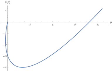
Figure 1: There are regions in the phase space $(\epsilon,p)$ of the quantum Yang-Mills states (18) where $\epsilon$ and $p$ are positive, where $p$ is positive and $\epsilon$ is negative and where they are both negative.

The energy density $\epsilon({\cal F})$ has its minimum outside of the perturbative vacuum state ${\cal F}=0$ at the Lorentz and renormalisation group invariant field strength [4]

$$2g^{2}{\cal F}_{vac}=\mu^{4}\exp{(-{96\pi^{2}\over b\ g^{2}(\mu)})}=\Lambda^{4}_{YM},$$ (17)

which characterises the dynamical breaking of scaling invariance of YM theory (13):

$$T^{\mu}_{\mu}=-{b\over 48\pi^{2}}2g^{2}{\cal F}_{vac}.$$

Thus the equation of state (30) will take the following form:

$$\epsilon({\cal F})=~{}{b\ g^{2}\over 96\pi^{2}}{\cal F}\Big{(}\ln{2g^{2}{\cal F}\over\Lambda^{4}_{YM}}-1\Big{)},~{}~{}~{}~{}~{}~{}~{}~{}~{}~{}p({\cal F})=~{}{1\over 3}{b\ g^{2}\over 96\pi^{2}}{\cal F}\Big{(}\ln{2g^{2}{\cal F}\over\Lambda^{4}_{YM}}+3\Big{)}.$$ (18)

By expressing the vacuum field strength tensor ${\cal F}$ in terms of vacuum pressure ${\cal F}={\cal F}(p)$ and substituting it into the vacuum energy density we will get the equation of state in the form $\epsilon=\epsilon(p)$ shown in Fig.1. In the limit $2g^{2}{\cal F}\gg\Lambda^{4}_{YM}$ (18) reduces to a radiation equation of state: $p=\epsilon/3.$ There are regions in the phase space of states $(\epsilon,p)$ where $\epsilon$ and $p$ are positive, where $p$ is positive and $\epsilon$ is negative and where they are both negative, as it is shown in Fig. 1. The pressure is always higher than in the case of radiation equation of state:

$$p={1\over 3}\epsilon+{4\over 3}{b\ g^{2}{\cal F}\over 96\pi^{2}}\Lambda^{4}_{YM}~{}~{}~{}~{}~{}\text{and}~{}~{}~{}~{}~{}w={p\over\epsilon}={\ln{2g^{2}{\cal F}\over\Lambda^{4}_{YM}}+3\over 3\Big{(}\ln{2g^{2}{\cal F}\over\Lambda^{4}_{YM}}-1\Big{)}}.$$ (19)

Our aim now is to analyse the Friedmann cosmology that is driven by the gauge field theory vacuum equation of state (18). The equations of general relativity in the presence of the vacuum energy momentum tensor (13) has the following form:

$$R_{\mu\nu}-{1\over 2}g_{\mu\nu}R={8\pi G\over c^{4}}\Big{[}T^{YM}_{\mu\nu}\Big{(}1+{b\ g^{2}\over 96\pi^{2}}\ln{2g^{2}{\cal F}\over\mu^{4}}\Big{)}-g_{\mu\nu}{b\ g^{2}\over 96\pi^{2}}{\cal F}\Big{]}.$$ (20)

The induced effective cosmological term can be expressed in terms of vacuum energy density (18) and vacuum field (17) as

$$\Lambda_{eff}={8\pi G\over 3c^{4}}~{}\epsilon_{vac}=-{8\pi G\over 3c^{4}}{b\over 192\pi^{2}}2g^{2}{\cal F}_{vac}=-{8\pi G\over 3c^{4}}{b\over 192\pi^{2}}\Lambda^{4}_{YM}~{}.$$ (21)

During the cosmological evolution the field strength tensor ${\cal F}$ will not stay permanently in its AdS ground state (17), (21) but will roll out through the well-defined trajectory in the phase space of states $(\epsilon,p)$ shown in Fig.1 that is defined by the Friedmann equations (1) and (3), (4).

The Yang-Mills energy momentum tensor $T_{\mu\nu}$ in (13), (15) has a diagonal homogeneous form, while the energy momentum tensor $T^{QED}_{\mu\nu}$ in QED is inhomogeneous due to the term $-E_{i}E_{j}-H_{i}H_{j}$ in (23) and it is a critical barrier for a successful vector field driven cosmology and inflation [115, 101]. The reason for this essential difference between QED and Yang Mills theory is that in Yang Mills theory the energy momentum tensor $T^{YM}_{\mu\nu}$ is homogeneous on the time dependent solutions $A^{a}_{i}(t)$ of Yang-Mills equations [75, 76, 77, 79] and therefore opens a room of possibilities for a vector field driven cosmology and inflation [3]. The space homogeneous gauge fields are described by a classical mechanical system, so called Yang-Mills classical mechanics (YMCM) [75, 76, 77, 79, 78, 80, 81, 82, 84, 85, 86, 87, 88, 89, 90, 91, 92, 93, 95, 96, 97, 98, 99], it represents the bosonic part of the matrix models [85, 86, 81, 87, 88, 89, 90, 91] and were considered in the context of the cosmological models in [109, 110, 111, 112, 113, 114, 115, 116, 117, 118, 119, 108, 106, 107, 108].

The chromoelectric and chromomagnetic fields have the following form:

$$E^{a}_{i}=G^{a}_{0i},~{}~{}~{}H^{a}_{i}={1\over 2}\epsilon_{ijk}G^{a}_{jk},~{}~{}~{}~{}~{}~{}~{}G^{a}_{0i}=\dot{A}^{a}_{i},~{}~{}~{}G^{a}_{jk}=g\epsilon^{abc}A^{b}_{j}A^{c}_{k}$$ (22)

and the components of the energy momentum tensor therefore are:

$$T_{00}={1\over 2}(E^{a}_{i})^{2}+{1\over 2}(H^{a}_{i})^{2},~{}~{}~{}T_{0i}=\epsilon_{ijk}E^{a}_{j}H^{a}_{k},~{}~{}~{}T_{ij}={1\over 2}\delta_{ij}(E^{a}_{i}E^{a}_{i}+H^{a}_{i}H^{a}_{i})-E^{a}_{i}E^{a}_{j}-H^{a}_{i}H^{a}_{j}.$$ (23)

The ”white colour” solution found in [75] has the form

$$A^{a}_{i}=\delta^{a}_{i}f(t),$$ (24)

and the corresponding chromoelectric and chromomagnetic fields take the following form:

$$E^{a}_{i}=\delta^{a}_{i}\dot{f}(t),~{}~{}~{}~{}H^{a}_{i}=g\delta^{a}_{i}f^{2}(t).$$ (25)

The energy density therefore is:

$$\epsilon=T_{00}={3\over 2}(\dot{f}^{2}+g^{2}f^{4})=\mu^{4},$$ (26)

where $\mu^{4}$ is a constant of dimension $mass^{4}$. Unusual property of this solution is that the chromoelectric and chromomagnetic fields are parallel to each other (25) and therefore the energy flux, the Pyonting vector, vanishes [75]

$$T_{0i}=S_{i}=\epsilon_{ijk}E^{a}_{j}H^{a}_{k}=0.$$ (27)

Thus importantly the space components of $T_{\mu\nu}$ in (23) are diagonal:

$$T_{ij}={1\over 2}\delta_{ij}\Big{(}\dot{f}^{2}+g^{2}\dot{f}^{4}\Big{)}=\delta_{ij}p.$$ (28)

The full energy momentum tensor has the form of a relativistic matter:

$$T_{\mu\nu}=\begin{pmatrix}\epsilon&0&0&0\\ 0&p&0&0\\ 0&0&p&0\\ 0&0&0&p\end{pmatrix}.$$ (29)

It follows from relations (26), (27) and (28) that the classical Yang Mills equation of state is equivalent to a homogeneous relativistic matter

$$p={1\over 3}\epsilon.$$ (30)

As we have seen above there are quantum corrections to the classical equation of the state (30) given by the first formula in (19)

$$p={1\over 3}\epsilon+{4\over 3}{b\ g^{2}{\cal F}\over 96\pi^{2}}\Lambda^{4}_{YM}.$$ (31)

In the subsequent sections we will investigate the solutions of the Friedmann equations in the universe that if filled out by the gauge field theory vacuum fluctuations described by the quantum equation of state (18), (19), (31) [3].

4 Quantum Yang-Mills Equation of State in Friedmann Cosmology

The time derivative of the energy density given in (18) is

$$\dot{\epsilon}={\cal B}~{}(2g^{2}\dot{{\cal F}})~{}\log{2g^{2}{\cal F}\over\Lambda^{4}_{YM}},$$ (32)

where $\dot{{\cal F}}={d{\cal F}/cdt}$. The time evolution of the energy density $\epsilon$ in (3) depends on the sign of the sum $\epsilon+p$. By using the expressions for $\epsilon$ and $p$ in (18) for the sum $\epsilon+p$ we will obtain:

$$\epsilon+p={4{\cal B}\over 3}~{}(2g^{2}{\cal F})~{}\log{2g^{2}{\cal F}\over\Lambda^{4}_{YM}},$$ (33)

where ${\cal B}$ is the coefficient of the one-loop $\beta(g)$ function:

$${\cal B}={b\over 192\pi^{2}}={11N-2N_{f}\over 192\pi^{2}}.$$ (34)

It follows that for $2g^{2}{\cal F}<\Lambda^{4}_{YM}$ the weak energy dominance condition $\epsilon+p\geq 0$ is violated. The equation (3) now takes the form

$$2g^{2}\dot{{\cal F}}+4(2g^{2}{\cal F}){\dot{a}\over a}=0$$ (35)

and can be integrated yielding

$$2g^{2}{\cal F}~{}a^{4}=const\equiv\Lambda^{4}_{YM}\ a^{4}_{0},$$ (36)

where the integration constant is parametrised in terms of the initial data parameter $a_{0}$. The energy density and pressure (18) can now be expressed in terms of the scale factor $a(t)$:

$$\epsilon={\cal B}{a^{4}_{0}\over a^{4}}\Big{(}\log{{a^{4}_{0}\over a^{4}}}-1\Big{)}\Lambda^{4}_{YM},~{}~{}~{}~{}~{}p={\cal B}{a^{4}_{0}\over 3a^{4}}\Big{(}\log{{a^{4}_{0}\over a^{4}}}+3\Big{)}\Lambda^{4}_{YM}.$$ (37)

With the help of the last expression for the $\epsilon$ the first Friedmann equation (1) will take the following form:

$${da\over cdt}=\pm\sqrt{{8\pi G\over 3c^{4}}~{}{\cal B}~{}\Lambda^{4}_{YM}~{}{a^{4}_{0}\over a^{2}}\Big{(}\log{{a^{4}_{0}\over a^{4}}}-1\Big{)}-k},~{}~{}~{}~{}~{}~{}~{}~{}k=0,\pm 1.$$ (38)

It is convenient to define the length scale $L$ as it appears naturally in (21) and (38):

$${1\over L^{2}}={8\pi G\over 3c^{4}}\ {\cal B}\ \Lambda^{4}_{YM}\equiv\Lambda_{eff}~{},$$ (39)

so the equation (38) will take the following form:

$${da\over cdt}=\pm\sqrt{{a^{2}_{0}\over L^{2}}~{}{a^{2}_{0}\over a^{2}}\Big{(}\log{{a^{4}_{0}\over a^{4}}}-1\Big{)}-k}.$$ (40)

In order to simplify the evolution equations further it is convenient to introduce the dimensionless scale factor $\tilde{a}$ and the dimensionless time variable $\tau$:

$$a(\tau)=a_{0}~{}\tilde{a}(\tau),~{}~{}~{}~{}ct=L~{}\tau,~{}$$ (41)

where we normalise the scale factor $a(\tau)$ to the constant parameter $a_{0}$ in (36). In these variables the evolution equation (40) is in its final form:

$${d\tilde{a}\over d\tau}=\pm\sqrt{{1\over\tilde{a}^{2}}\Big{(}\log{{1\over\tilde{a}^{4}}}-1\Big{)}-k\gamma^{2}},~{}~{}~{}~{}~{}~{}k=0,\pm 1,~{}~{}~{}~{}~{}~{}~{}~{}\gamma^{2}=\Big{(}{L\over a_{0}}\Big{)}^{2}.$$ (42)

The evolution equation (42) can be represented in terms of the dimensionless conformal time $\eta$:

$$cdt=L~{}d\tau=a(\eta)d\eta=a_{0}\tilde{a}d\eta,$$ (43)

as well as (the prime denotes the differentiation with respect to $\eta$):

$$\tilde{a}^{{}^{\prime}}\equiv{d\tilde{a}\over d\eta}=\pm\sqrt{{1\over\gamma^{2}}\Big{(}\log{{1\over\tilde{a}^{4}}}-1\Big{)}-k~{}\tilde{a}^{2}}.$$ (44)

The evolution equations (42) and (44) should be investigated in six regions of the two-dimensional parameter space $(a_{0},\Lambda_{YM})$. The numerical value of $\gamma^{2}$ defines the relation $a^{2}_{0}={1\over\gamma^{2}}L^{2}(\Lambda_{YM})$ between basic independent parameters $a_{0}$ and $\Lambda_{YM}$ through the equations (42) and (39). Thus the corresponding six regions in the parameter space are defined in terms of $\gamma^{2}$:

$$k=-1,~{}~{}~{}~{}0\leq\gamma^{2}<\gamma^{2}_{c}~{}~{}~{}~{}~{}~{}~{}~{}~{}~{}~{}~{}~{}~{}\text{Regions I ($\tilde{a}\leq\mu_{1}$) and II ($\mu_{2}\leq\tilde{a}$)}$$

$$k=-1,~{}~{}~{}~{}\gamma^{2}=\gamma^{2}_{c}={2\over\sqrt{e}}~{}~{}~{}~{}~{}~{}~{}~{}~{}~{}~{}\text{Region III (separatrix, $\tilde{a}\leq\mu_{c}$)}$$

$$k=-1,~{}~{}~{}~{}\gamma^{2}_{c}<\gamma^{2}~{}~{}~{}~{}~{}~{}~{}~{}~{}~{}~{}~{}~{}~{}~{}~{}~{}~{}~{}~{}\text{Regions IV ($0\leq\tilde{a}$)}$$ (45)

$$k=0,~{}~{}~{}~{}~{}~{}~{}$$

$$k=1,~{}~{}~{}~{}~{}~{}~{}0\leq\gamma^{2}.$$

In terms of scale factor $\tilde{a}$ and time variable $\tau$ (41) the field strength tensor (36) has the following form:

$$2g^{2}{\cal F}~{}={\Lambda^{4}_{YM}\over\tilde{a}^{4}(\tau)}$$ (46)

and the energy density and the pressure (37) will take the form

$$\epsilon={{\cal B}\over\tilde{a}^{4}(\tau)}\Big{(}\log{{1\over\tilde{a}^{4}(\tau)}}-1\Big{)}\Lambda^{4}_{YM},~{}~{}~{}~{}~{}~{}~{}p={{\cal B}\over 3\tilde{a}^{4}(\tau)}\Big{(}\log{{1\over\tilde{a}^{4}(\tau)}}+3\Big{)}\Lambda^{4}_{YM}.$$ (47)

There is a straightforward relation between energy density, pressure and the barotropic parameter $w$:

$$p={1\over 3}\epsilon+{4\over 3}{{\cal B}\over\tilde{a}^{4}(\tau)}\Lambda^{4}_{YM},~{}~{}~{}~{}~{}~{}~{}~{}~{}w={p\over\epsilon}={\log{{1\over\tilde{a}^{4}(\tau)}}+3\over 3\Big{(}\log{{1\over\tilde{a}^{4}(\tau)}}-1\Big{)}}.$$ (48)

In the next sections we will investigate the solutions of the equation (42) and the time evolution of the field strength tensor (46), of the energy density and the pressure (47 ). We can also extract the Hubble parameter from (1) by using (42)

$$L^{2}H^{2}=L^{2}\Big{(}{\dot{a}\over a}\Big{)}^{2}={1\over\tilde{a}^{2}}\Big{(}{d\tilde{a}\over d\tau}\Big{)}^{2}={1\over\tilde{a}^{4}(\tau)}\Big{(}\log{1\over\tilde{a}^{4}(\tau)}-1\Big{)}-{k\gamma^{2}\over\tilde{a}^{2}(\tau)}$$ (49)

and the corresponding deceleration parameter

$$q=-{\ddot{a}\over a}{1\over H^{2}}.$$ (50)

The acceleration is determined by the right-hand side of the equation (4) and is proportional to $\epsilon+3p$, which is:

$$\epsilon+3p=2{\cal B}~{}(2g^{2}{\cal F})~{}\Big{(}\log{2g^{2}{\cal F}\over\Lambda^{4}_{YM}}+1\Big{)}.$$ (51)

Similar to the case of the scalar field driven evolution (10) here as well for the fields $2g^{2}{\cal F}<{1\over e}\Lambda^{4}_{YM}$ the strong energy dominance condition $\epsilon+3p\geq 0$ is violated. From acceleration Friedmann equation (4) and (47 ) we have

$$L^{2}{\ddot{a}\over a}=-{1\over\tilde{a}^{4}}\Big{(}\log{1\over\tilde{a}^{4}}+1\Big{)}.$$ (52)

Thus for $q$ with the help of (49) we will get

$$q={{1\over\tilde{a}^{4}}\Big{(}\log{1\over\tilde{a}^{4}}+1\Big{)}\over{1\over\tilde{a}^{4}}\Big{(}\log{1\over\tilde{a}^{4}}-1\Big{)}-{k\gamma^{2}\over\tilde{a}^{2}}}$$ (53)

and for the density parameter $\Omega_{vac}$ the following expression:

$$\Omega_{vac}\equiv{8\pi G\over 3c^{4}}{\epsilon\over H^{2}}={1\over L^{2}H^{2}}~{}{1\over\tilde{a}^{4}}\Big{(}\log{1\over\tilde{a}^{4}}-1\Big{)},$$ (54)

where we used (47 ), (39). By using the equation (49) $\Omega_{vac}$ can be expressed also in the following form:

$$\Omega_{vac}-1=k{\gamma^{2}\over L^{2}H^{2}\tilde{a}^{2}}=k{\gamma^{2}\over({d\tilde{a}\over d\tau})^{2}}.$$ (55)

We will investigate these observables in the two-dimensional parameter space $(a_{0},\Lambda_{YM})$ in each of the six regions (4). As we mentioned above, the parameter $\gamma^{2}={L^{2}\over a^{2}_{0}}$ is a function of $a_{0}$ and $\Lambda_{YM}$, the basic parameters defining the evolution of the Friedmann equations in the case of gauge field theory vacuum polarisation. We will start our analysis by considering the $k=-1$ geometry.

5 The Parameter Space of the Type I-IV Solutions

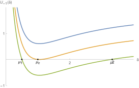
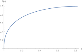
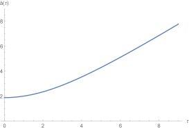
Figure 2: The behaviour of the potential $U_{-1}(\tilde{a})$ (57) is shown in the left figure. When the parameter $\gamma^{2}$ is in the interval $0\leq\gamma^{2}<{2\over\sqrt{e}}$, there are two solutions of the equation $U_{-1}(\mu_{i})=0,~{}i=1,2$, that define the Region I, where $\tilde{a}\in[0,\mu_{1}]$ and the Region II, where $\tilde{a}\in[\mu_{2},\infty]$.  When $\gamma^{2}=\gamma^{2}_{c}={2\over\sqrt{e}}$, there is only one solution of the equation $U_{-1}(\mu_{c})=0$ that defines the Region III, where $\tilde{a}\in[0,\mu_{c}]$. When ${2\over\sqrt{e}}<\gamma^{2}$, the potential is always positive $U_{-1}(\tilde{a})>0$ and the Region IV is where $\tilde{a}\in[0,\infty]$. In particular, when $\gamma^{2}=1$, $\mu_{1}\simeq 1$ and the scale factor $\tilde{a}(\tau)$ of the Type I solution is bounded $\tilde{a}\in[0,\mu_{1}]$. Its evolution time is finite $\tau\in[0,2\tau_{m}]$, where $\tau_{m}\simeq 0.83$ is a half period. The figure in the middle shows the behaviour of the Type I solution. The Type II solution shown in the right figure is unbounded $\tilde{a}\in[\mu_{2},\infty]$, where $\mu_{2}\simeq 1.87$ and $\tau\in[0,\infty]$. The Type II solution initially grows exponentially because the deceleration parameter is negative, $q<0$. At late time the regime of exponential expansion continuously transforms into a linear in time growth of the scale factor.

In case of $k=-1$ geometry the equation (42) takes the following form:

$${d\tilde{a}\over d\tau}=\pm\sqrt{{1\over\tilde{a}^{2}}\Big{(}\log{{1\over\tilde{a}^{4}}}-1\Big{)}+\gamma^{2}},~{}~{}~{}~{}\text{where}~{}~{}~{}~{}~{}0\leq\gamma^{2},$$ (56)

and the corresponding ”potential” function $U_{-1}(\tilde{a})$ shown in Fig.2 is:

$$U_{-1}(\tilde{a})\equiv{1\over\tilde{a}^{2}}\Big{(}\log{{1\over\tilde{a}^{4}}}-1\Big{)}+\gamma^{2}.$$ (57)

The solution of the equation $U_{-1}(\mu)=0$ determines the values of the scale factor $\tilde{a}=\mu$ at which the square root changes its sign. The evolution equation (56) should be restricted to those real values of $\tilde{a}$ at which the potential $U_{0}(\tilde{a})$ is nonnegative. Thus the equation $U_{-1}(\mu)=0$ defines the boundary values of the scale factor $\tilde{a}=\mu$:

$${1\over\mu^{2}}\Big{(}\log{{1\over\mu^{4}}}-1\Big{)}+\gamma^{2}=0.~{}~{}~{}~{}$$ (58)

The behaviours of the solutions depending on the value of the parameter $\gamma^{2}$. When

$$0\leq\gamma^{2}<\gamma^{2}_{c}\equiv{2\over\sqrt{e}},$$ (59)

there are two solutions $\tilde{a}_{1}=\mu_{1}$ and $\tilde{a}_{2}=\mu_{2}$ of the above equation that are defining the regions where the potential $U_{-1}(\tilde{a})$ is positive. In the first region $I$ we have $\tilde{a}\in[0,\mu_{1}]$, and in the second region $II$ $\tilde{a}\in[\mu_{2},\infty]$. These two regions are shown in Fig.2. The region $III$ appears when $\gamma^{2}=\gamma^{2}_{c}$ and it is the separatrix between regions $II$ and $IV$. At the separatrix point $\gamma^{2}=\gamma^{2}_{c}$ the equation $U_{-1}(\mu)=0$ has only one solution $\tilde{a}=\mu_{c}$ and the scale factor $\tilde{a}$ takes its values in the maximally available interval $\tilde{a}\in[0,\mu_{c}]$. Finally, in the region $IV$, where $\gamma^{2}_{c}<\gamma^{2}$, the potential function $U_{-1}(\tilde{a})$ is always positive for all values of $\tilde{a}$ and the scale factor takes its values in the whole interval $\tilde{a}\in[0,\infty]$. We will consider these four regions separately.

6 Type I Solution

Let’s consider first the Type $I$ solution when $0\leq\gamma^{2}<\gamma^{2}_{c}$ and $\tilde{a}\leq\mu_{1}$. The equation (58) can be solved by the substitution

$$\gamma^{2}\mu^{2}=2u$$ (60)

that reduces the equation (58) to the Lamber-Euler type [71, 72, 73]:

$$~{}~{}~{}~{}ue^{-u}={\gamma^{2}\over 2\sqrt{e}}.$$ (61)

The solution is expressible in terms of $W_{0}(x)$ function which is defined for negative values of its argument in the interval $-1/e<x\leq 0$ and is acquiring negative values $-1<W_{0}(x)\leq 0$. The solution takes the following form (see Appendix A):

$$u=-W_{0}\Big{(}-{\gamma^{2}\over 2\sqrt{e}}\Big{)}.$$ (62)

The maximal value of the scale factor $\tilde{a}$ therefore is

$$\mu^{2}_{1}=-{2\over\gamma^{2}}~{}W_{0}\Big{(}-{\gamma^{2}\over 2\sqrt{e}}\Big{)},~{}~{}~{}~{}$$ (63)

and it follows that (see Appendix)

$${1\over\sqrt{e}}\leq\mu^{2}_{1}<\sqrt{e},~{}~{}~{}~{}~{}~{}\gamma^{2}\mu^{2}_{1}<2.$$ (64)

The interval in which $\tilde{a}$ takes its values is:

$$~{}~{}~{}\tilde{a}\in[0,\mu_{1}].$$ (65)

With the next substitution

$$\tilde{a}^{4}=\mu^{4}_{1}e^{-b^{2}},~{}~{}~{}~{}~{}b\in[-\infty,\infty],$$ (66)

the equation (56) will reduce to the following form:

$${db\over d\tau}={2\over\mu^{2}_{1}}~{}e^{{b^{2}\over 2}}\Big{(}1-{\gamma^{2}\mu^{2}_{1}\over b^{2}}(1-e^{-{b^{2}\over 2}}\Big{)}^{1/2}.$$ (67)

With the boundary condition $b(0)=-\infty$ at $\tau=0$ we will get the integral representation of the function $b(\tau)$:

$$\int^{b(\tau)}_{-\infty}{dbe^{-{b^{2}\over 2}}\over\Big{(}1-{\gamma^{2}\mu^{2}_{1}\over b^{2}}(1-e^{-{b^{2}\over 2}}\Big{)}^{1/2}}~{}={2\over\mu^{2}_{1}}~{}\tau.$$ (68)

Within a finite-time interval after the initial expansion the universe will approach its maximal size $\mu_{1}$ and then begin to recontract. This time interval $\tau\in[0,\tau_{m}]$ is defined by the integral

$$\int^{0}_{-\infty}{dbe^{-{b^{2}\over 2}}\over\Big{(}1-{\gamma^{2}\mu^{2}_{1}\over b^{2}}(1-e^{-{b^{2}\over 2}}\Big{)}^{1/2}}~{}={2\over\mu^{2}_{1}}~{}\tau_{m}$$ (69)

and is equal to the half of the total period, which is equal to $2\tau_{m}$. Thus during the time evolution $\tilde{a}(\tau)$ is reaching its maximal value $\tilde{a}=\mu_{1}$ at $\tau_{m}$ and then contracting to zero value at $\tau=2\tau_{m}$. The asymptotic behaviour of the $\tilde{a}(\tau)$ near $\tau=\tau_{m}$ and $\tau=0$ has the form

$$\tilde{a}(\tau)\simeq\begin{cases}\mu_{1}-{2-\gamma^{2}\mu^{2}_{1}\over 2\mu^{3}_{1}}(\tau-\tau_{m})^{2},~{}~{}~{}~{}~{}\tau\rightarrow\tau_{m}\\ \tau^{1/2}\ln^{1/4}{1\over\tau^{1/2}},~{}~{}~{}~{}~{}~{}~{}~{}~{}~{}~{}~{}~{}\tau\rightarrow 0\end{cases}.$$ (70)

At the initial stages of the expansion and the final stages of the contraction the metric is singular $\tilde{a}(t)\propto~{}t^{1/2}\ln^{1/4}{1\over t^{1/2}}$. Up to the logarithmic term the singularity is similar to that in the cosmological models with relativistic matter where $\tilde{a}(t)\propto~{}t^{1/2}$. The difference is that here the scale factor is periodic in time while in open cosmological model ($k=-1$) with relativistic matter the expansion is eternal. Thus when $a^{2}_{0}>L^{2}/\gamma^{2}_{c}$ (59), the vacuum energy density $\epsilon$ is able to reverse the initial expansion shown in Fig.2.

The field strength (46) evolution in time is expressible in terms of $b(\tau)$ function:

$$2g^{2}{\cal F}={e^{b^{2}(\tau)}\over\mu^{4}_{1}}\Lambda^{4}_{YM}.$$ (71)

The minimum value of the field strength (71) at $\tau=\tau_{m}$ ($b=0$) is

$$2g^{2}{\cal F}_{m}={1\over\mu^{4}_{1}}\Lambda^{4}_{YM},~{}~{}~{}~{}$$ (72)

and from (63), (64) it follows that the minimum value of the field strength varies in the interval

$${1\over e}\Lambda^{4}_{YM}<2g^{2}{\cal F}_{m}\leq e\Lambda^{4}_{YM}$$ (73)

when $\gamma^{2}\in[0,\gamma^{2}_{c})$. The energy density and pressure (47) will evolve in time as well:

$$\epsilon={{\cal B}\over\mu^{4}_{1}}e^{b^{2}(\tau)}\Big{(}b^{2}(\tau)-\gamma^{2}\mu^{2}_{1}\Big{)}\Lambda^{4}_{YM},~{}~{}~{}p={{\cal B}\over 3\mu^{4}_{1}}e^{b^{2}(\tau)}\Big{(}b^{2}(\tau)-\gamma^{2}\mu^{2}_{1}+4\Big{)}\Lambda^{4}_{YM}.$$ (74)

The equation of state will take the following form:

$$p={\epsilon\over 3}+~{}{4{\cal B}e^{b^{2}(\tau)}\over 3\mu^{4}_{1}}\Lambda^{4}_{YM}~{}>~{}{\epsilon\over 3},~{}~{}~{}~{}~{}~{}~{}~{}~{}~{}w_{I}={p\over\epsilon}={b^{2}(\tau)-\gamma^{2}\mu^{2}_{1}+4\over 3\Big{(}b^{2}(\tau)-\gamma^{2}\mu^{2}_{1}\Big{)}}$$ (75)

showing that the pressure is larger than that in the case of radiation and $w_{I}\in(-1,{1\over 3})$. The values of the energy density and pressure at $\tau=\tau_{m}$ are

$$\epsilon_{m}=-{\cal B}{\gamma^{2}\mu^{2}_{1}\over\mu^{4}_{1}}\Lambda^{4}_{YM},~{}~{}~{}~{}~{}p_{m}={\cal B}{4-\gamma^{2}\mu^{2}_{1}\over 3\mu^{4}_{1}}\Lambda^{4}_{YM}.$$ (76)

The deceleration parameter in Type I case is positive

$$q_{I}={b^{2}+2-\gamma^{2}\mu^{2}_{1}\over b^{2}-\gamma^{2}\mu^{2}_{1}(1-e^{-b^{2}/2})}\geq 1,$$ (77)

where $\gamma^{2}\mu^{2}_{1}<2$ (64). The Hubble parameter and the density parameter $\Omega$ (54), (55) are:

$$L^{2}H^{2}={e^{b^{2}}\over\mu^{4}_{1}}\Big{(}b^{2}-\gamma^{2}\mu^{2}_{1}(1-e^{-b^{2}/2})\Big{)},~{}~{}~{}~{}\Omega_{I}-1=-{\gamma^{2}\mu^{2}_{1}e^{-b^{2}/2}\over b^{2}-\gamma^{2}\mu^{2}_{1}(1-e^{-b^{2}/2})}.$$ (78)

At the typical value of $\gamma^{2}=1$ $\mu^{2}_{1}=-2W_{0}(-{1\over 2\sqrt{e}})=1$ and $\tau_{m}\simeq 0.83$. With the help of the formulas (43) and (39) one can get a numerical estimate of the expansion proper time interval:

$$ct_{m}=\tau_{m}L\simeq 1.03\times 10^{25}\Big{(}{eV\over\Lambda_{YM}}\Big{)}^{2}~{}cm,$$ (79)

where $L=1.25\times 10^{25}\Big{(}{eV\over\Lambda_{YM}}\Big{)}^{2}cm$. In comparison, the Hubble length is $cH^{-1}_{0}\simeq 1.37\times 10^{28}cm$. The physical meaning of this result is that the Yang-Mills vacuum energy density $\epsilon$ is able to reverse the expansion earlier than the Hubble time. In order to be consistent with the cosmological observational data when Type I solution is analysed one should have a typical energy scale of the dimensional transmutation in Yang-Mills theory $\Lambda_{YM}$ to be constrained by a few electronvolt: $\Lambda_{YM}\sim eV$. This scenario can be realised if the Callan-Symanzik beta-function coefficient ${\cal B}$ in (34), is effectively small, like in conformal gauge field theories, and therefore the scale $L$ is large enough:

$$L^{2}={3c^{4}\over 8\pi G}\ {1\over{\cal B}\ \Lambda^{4}_{YM}}\rightarrow\infty,~{}~{}~{}~{}~{}{\cal B}\rightarrow 0.$$ (80)

Considering $\Lambda_{YM}$ in (39) to be one of the fundamental interaction scales we obtain the following lengths:

$$L_{QCD}\sim 10^{9}cm,~{}~{}~{}~{}~{}L_{EW}\sim 10^{3}cm,~{}~{}~{}~{}~{}L_{GUT}\sim 10^{-25}cm,~{}~{}~{}~{}~{}L_{Pl}\sim 10^{-31}cm.$$ (81)

These scales lead to a much shorter universe live-time, but, importantly, to finite non-diverging time intervals . In the case of Type II solution to be considered in the next section, when $0\leq\gamma^{2}<\gamma^{2}_{c}$ and $\tilde{a}(0)\geq\mu_{2}$, the deceleration parameter $q$ is negative and the scale factor grows exponentially with the inflation of a finite duration (97 ) that undergoes a continuous transition to a linear in time growth (99).

7 Type II Solution

For the Type $II$ solution we have $0<\gamma^{2}<{2\over\sqrt{e}}$ and $\tilde{a}\geq\mu_{2}$. The Lamber-Euler equation (61)

$$~{}~{}~{}~{}ue^{-u}={\gamma^{2}\over 2\sqrt{e}}$$

has an alternative solution expressible in terms of $W_{-}(x)$ function, which represents the other branch of the general $W(x)$ function of the real argument $x$ (see Appendix A). For the negative values of the argument in the interval $-1/e\leq x\leq 0$ the function acquires negative values in the interval $-\infty\leq W_{-}(x)\leq-1$. Thus the solution takes the following form:

$$u=-W_{-}\Big{(}-{\gamma^{2}\over 2\sqrt{e}}\Big{)}.$$

The minimal value of the scale factor (60) therefore is

$$\mu^{2}_{2}=-{2\over\gamma^{2}}~{}W_{-}\Big{(}-{\gamma^{2}\over 2\sqrt{e}}\Big{)},~{}~{}~{}~{}~{}~{}$$ (82)

and it follows that (see Appendix A)

$$\sqrt{e}<\mu^{2}_{2}\leq\infty,~{}~{}~{}~{}~{}~{}~{}~{}~{}~{}2<\gamma^{2}\mu^{2}_{2}.$$ (83)

The interval in which $\tilde{a}$ takes its values is now infinite:

$$~{}~{}~{}\tilde{a}\in[\mu_{2},\infty].$$ (84)

With the substitution

$$\tilde{a}^{4}=\mu^{4}_{2}e^{b^{2}},~{}~{}~{}~{}~{}b\in[0,\infty],$$ (85)

the equation (56) will take the following form:

$${db\over d\tau}={2\over\mu^{2}_{2}}~{}e^{-{b^{2}\over 2}}\Big{(}{\gamma^{2}\mu^{2}_{2}\over b^{2}}(e^{{b^{2}\over 2}}-1)-1\Big{)}^{1/2}.$$ (86)

With the boundary conditions at $\tau=0$ where $b(0)=0$ ($\tilde{a}(0)=\mu_{2}$) we will get the integral representation of the function $b(\tau)$:

$$\int^{b(\tau)}_{0}{db~{}e^{{b^{2}\over 2}}\over\Big{(}{\gamma^{2}\mu^{2}_{2}\over b^{2}}(e^{{b^{2}\over 2}}-1)-1\Big{)}^{1/2}}~{}={2\over\mu^{2}_{2}}~{}\tau.$$ (87)

The time interval is $\tau\in[0,\infty]$, and as $\tau\rightarrow\infty$, we have

$$b^{2}(\tau)\simeq 4\ln{\gamma\over\mu_{2}}\tau,~{}~{}~{}~{}~{}~{}a=a_{0}\tilde{a}\simeq a_{0}\gamma\tau=ct.$$ (88)

The field strength evolution in time is expressible in terms of $b(\tau)$ function:

$$2g^{2}{\cal F}={e^{-b^{2}(\tau)}\over\mu^{4}_{2}}\Lambda^{4}_{YM}.$$ (89)

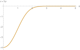
Figure 3: The r.h.s $\epsilon+3p$ of the Friedmann acceleration equation (4) always negative in the case of Type II solution (93).

The maximal value of the field strength (46) is at $\tau=0$ where $b(0)=0$:

$$2g^{2}{\cal F}_{m}={1\over\mu^{4}_{1}}\Lambda^{4}_{YM},~{}~{}~{}~{}$$ (90)

and from (83 )

$$0\leq 2g^{2}{\cal F}_{m}<{1\over e}\Lambda^{4}_{YM}.$$ (91)

The behaviour of the energy density and pressure is:

$$\epsilon=-{{\cal B}\over\mu^{4}_{2}}e^{-b^{2}(\tau)}\Big{(}b^{2}(\tau)+\gamma^{2}\mu^{2}_{2}\Big{)}\Lambda^{4}_{YM},~{}~{}~{}p=-{{\cal B}\over 3\mu^{4}_{2}}e^{-b^{2}(\tau)}\Big{(}b^{2}(\tau)+\gamma^{2}\mu^{2}_{2}-4\Big{)}\Lambda^{4}_{YM},$$ (92)

and as $\tau\rightarrow\infty$ the energy density and pressure tend to zero values of the perturbative vacuum state. The right-hand side of the Friedmann acceleration equation (4) has the following form:

$$\epsilon+3p=-{2{\cal B}\over\mu^{4}_{2}}~{}e^{-b^{2}(\tau)}(b^{2}(\tau)+\gamma^{2}\mu^{2}_{2}-2)\Lambda^{4}_{YM},~{}~{}~{}~{}~{}~{}b\in[0,+\infty],$$ (93)

and is always negative Fig.3. At the initial stages of the expansion $\tau=0$ ($b=0$) the energy density and pressure are finite and the solution avoids a singular behaviour

$$a(0)=a_{0}~{}\tilde{a}(0)=a_{0}~{}\mu_{2}~{}e^{b(0)^{2}/4}=L{\mu_{2}\over\gamma}~{}>~{}0.$$

This behaviour of the scale factor can be compared with the nonsingular solution discussed in [12]. For the equation of state $p=w\epsilon$ one can find the behaviour of the effective parameter $w$

$$w_{II}={b^{2}(\tau)+\gamma^{2}\mu^{2}_{2}-4\over 3\Big{(}b^{2}(\tau)+\gamma^{2}\mu^{2}_{2}\Big{)}},~{}~{}~{}~{}~{}~{}~{}-1\leq w_{II},$$ (94)

where $b\in[0,\infty]$. The deceleration parameter of the Type II solution is always negative:

$$q_{II}={b^{2}+\gamma^{2}\mu^{2}_{2}-2\over b^{2}+\gamma^{2}\mu^{2}_{2}(1-e^{b^{2}/2})}<0$$ (95)

in the region II (83) where $2<\gamma^{2}\mu^{2}_{2}$. As it follows from (95) and (87), there is a period of strong acceleration

$$q_{II}\propto-{2\over b^{2}}$$ (96)

at the initial stages of the expansion $b^{2}\sim\tau$ and the scale factor (85) grows exponentially:

$$~{}~{}~{}~{}~{}~{}~{}a(t)\simeq L~{}{\mu_{2}\over\gamma}~{}\exp{\Big{[}{2\over\mu^{2}_{2}}~{}\sqrt{{\gamma^{2}\mu^{2}_{2}\over 2}-1}~{}{ct\over L}\Big{]}}.$$ (97)

The inflation is slowing down when $ct>L$ because $b^{2}$ increases and the acceleration drops:

$$q_{II}\propto-{b^{2}\over\gamma^{2}\mu^{2}_{2}}e^{-b^{2}/2}\rightarrow 0.$$ (98)

The regime of the exponential growth will continuously transformed into the linear in time growth of the scale factor

$$a(t)\simeq~{}ct,~{}~{}~{}~{}~{}~{}~{}a(\eta)\simeq a_{0}e^{\eta}.$$ (99)

The acceleration has its trace on the behaviour of Hubble parameter, which has the following form:

$$L^{2}H^{2}={e^{-b^{2}}\over\mu^{4}_{2}}\Big{(}\gamma^{2}\mu^{2}_{2}(e^{b^{2}/2}-1)-b^{2}\Big{)}.$$ (100)

The $L^{2}H^{2}$ is sharply increasing from zero value and reaches its maximum at

$$b^{2}_{s}=1-\gamma^{2}\mu^{2}_{2}-2W_{-1}\Big{(}-{\gamma^{2}\mu^{2}_{2}\over 4}\exp{({1-\gamma^{2}\mu^{2}_{2}\over 2})}\Big{)}$$ (101)

and allows to estimate its duration

$$\tau_{s}={\mu^{2}_{2}\over 2}\int^{9b_{s}}_{0}{db~{}e^{{b^{2}\over 2}}\over\Big{(}{\gamma^{2}\mu^{2}_{2}\over b^{2}}(e^{{b^{2}\over 2}}-1)-1\Big{)}^{1/2}}~{}.$$ (102)

The number of e-foldings for the time evolution from $\tau=0$ to $\tau_{s}$ is defined as ${\cal N}=\ln{a(\tau_{s})\over a(0)}.$ For the typical parameters around $\gamma^{2}=1.211$, $\mu^{2}_{2}\simeq 1.75$ we get $\tau_{s}=10^{23}$ and ${\cal N}\simeq 53$. The duration of the inflation in the case of the GUT scale $\Lambda_{YM}=\Lambda_{GUT}=10^{16}GeV$ is of order

$$t^{GUT}_{s}={L_{GUT}\over c}\tau_{s}\simeq 4.2\times 10^{-13}~{}sec,$$ (103)

where $L_{GUT}\simeq 1.25\times 10^{-25}cm$ as in (81). The initial and finale values of the scale factor are:

$$a(0)=L_{GUT}{\mu_{2}\over\gamma}\simeq 1.5\times 10^{-25}cm,~{}~{}~{}~{}~{}~{}a(t_{s})=L_{GUT}{\mu_{2}\over\gamma}e^{{\cal N}}\simeq 1.25\times 10^{-2}cm,$$

where $a(t_{s})$ is ”about the size of a marble” [13]. The density parameter $\Omega$ (54) has the following form

$$~{}\Omega_{vac}-1=-{\gamma^{2}\over({d\tilde{a}\over d\tau})^{2}}=-{\gamma^{2}\mu^{2}_{2}e^{b^{2}/2}\over\gamma^{2}\mu^{2}_{2}(e^{b^{2}/2}-1)-b^{2}}$$ (104)

and at $t\gg t_{s}$  ($b^{2}\rightarrow\infty$) the vacuum density tends to zero $\Omega_{vac}\rightarrow 0$ meaning that the influence of the gauge field theory vacuum on the evolution of the universe fades out turning into a linear expansion (99).

It seems natural to include the energy densities $\epsilon_{f}$ that can contribute into the total energy density $\epsilon=\sum\epsilon_{f}$ from the hierarchy of fundamental interaction scales. Taking into account the fact that at each scale (81) the acceleration has a finite duration (98) and appears at a different epoch of the universe expansion, its seems possible that a very large scale $\Lambda^{{}^{\prime}}_{YM}\gg GeV$ contributes to the inflation at the initial stages of the expansion and a smaller scale $\Lambda^{{}^{\prime\prime}}_{YM}\simeq eV$ contributes to the late-time acceleration of the universe. In addition here we do not include the energy density of the standard matter (5) that can be easily included, and the subsequent evolution of the universe will turn into the standard hot universe expansion. In the next section we will consider the Type III solution when the parameter $\gamma^{2}$ is equal to its critical value $\gamma^{2}=\gamma^{2}_{c}$.

8 Type III Solution (Separatrix)

Consider now the Type $III$ solution when $\gamma^{2}=\gamma^{2}_{c}={2\over\sqrt{e}}$. The Lamber-Euler equation (61)

$$~{}~{}~{}~{}ue^{-u}={\gamma^{2}_{c}\over 2\sqrt{e}}={1\over e}$$

in this case has a unique solution (see Appendix B)

$$u_{c}=-W_{0}(-{1\over e})=-W_{-}(-{1\over e})=1,$$

and from (60) we get

$$\mu^{2}_{c}={2u_{c}\over\gamma^{2}_{c}}=\sqrt{e}~{},~{}~{}~{}~{}~{}~{}~{}\mu^{2}_{c}\gamma^{2}_{c}=2.$$ (105)

The interval in which $\tilde{a}$ variates is now

$$~{}~{}~{}\tilde{a}\in[0,\mu_{c}].$$ (106)

When $\gamma^{2}\rightarrow\gamma^{2}_{c}$, the region I and region II (63) and (82) merge at $\mu^{2}_{1}=\mu^{2}_{2}\rightarrow\mu^{2}_{c}$, as one can see from (64), (83). With the substitution

$$\tilde{a}=\mu_{c}e^{b},~{}~{}~{}~{}~{}b\in[-\infty,0],$$ (107)

the equation (56) will take the following form:

$${db\over d\tau}=\sqrt{{2\over e}}~{}e^{-2b}\Big{(}e^{2b}-1-2b\Big{)}^{1/2}.$$ (108)

With the boundary conditions $b(0)=-\infty$ ($\tilde{a}(0)=0$) in place we will get the integral representation of the function $b(\tau)$:

$$\int^{b(\tau)}_{-\infty}{db~{}e^{2b}\over\Big{(}e^{2b}-1-2b\Big{)}^{1/2}}~{}=\sqrt{{2\over e}}~{}\tau,~{}~{}~{}~{}~{}~{}\tau\in[0,\infty].$$ (109)

The field strength evolution in time takes the following form:

$$2g^{2}{\cal F}=e^{-4b(\tau)-1}\Lambda^{4}_{YM}.$$ (110)

The behaviour of the energy density and pressure is:

$$\epsilon=2{\cal B}e^{-4b(\tau)-1}\Big{(}-2b(\tau)-1\Big{)}\Lambda^{4}_{YM},~{}~{}~{}~{}~{}~{}p={2{\cal B}\over 3}e^{-4b(\tau)-1}\Big{(}-2b(\tau)+1\Big{)}\Lambda^{4}_{YM}.$$ (111)

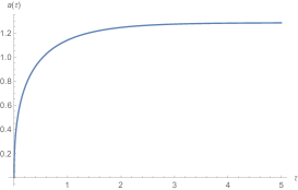
Figure 4: When $k=-1$ and $\gamma^{2}=\gamma^{2}_{c}={2\over\sqrt{e}}$, the Type III solution is approaching asymptotically the maximum value $\tilde{a}=\mu_{c}$ as $\tau\rightarrow\infty$.

There is a characteristic time $\tau=\tau_{0}$, corresponding to $b=-1/2$

$$\int^{-1/2}_{-\infty}{db~{}e^{2b}\over\Big{(}e^{2b}-1-2b\Big{)}^{1/2}}~{}=\sqrt{{2\over e}}~{}\tau_{0}$$ (112)

when the energy density approaches the zero value

$$2g^{2}{\cal F}_{0}=e\Lambda^{4}_{YM},~{}~{}~{}~{}~{}\epsilon_{0}=0,~{}~{}~{}~{}~{}p_{0}={4{\cal B}\over 3e}\Lambda^{4}_{YM}.$$ (113)

The scale factor asymptotically approaches a maximal static value shown in Fig.4

$$\tilde{a}=\mu_{c}e^{b}\rightarrow\mu_{c}$$ (114)

when $\tau\rightarrow\infty$ and $b\propto e^{-\sqrt{2}\tau}\rightarrow 0$ in (109). The energy density becomes negative in the region $b\in(-1/2,0]$. The field strength, energy density, and pressure are approaching asymptotically the following values:

$$2g^{2}{\cal F}_{c}={1\over e}\Lambda^{4}_{YM},~{}~{}~{}~{}~{}\epsilon_{c}=-{2{\cal B}\over e}\Lambda^{4}_{YM},~{}~{}~{}~{}~{}p_{c}={2{\cal B}\over 3e}\Lambda^{4}_{YM}.$$ (115)

According to the Friedmann equations (3)-(4) the acceleration is driven by the overall sign of the $\epsilon+3p$ that can be calculated by using the expressions (111)

$$\epsilon+3p=-8{\cal B}b(\tau)e^{-4b(\tau)-1}\Lambda^{4}_{YM}\geq 0,~{}~{}~{}~{}~{}~{}~{}~{}~{}~{}~{}b\in[-\infty,0].$$ (116)

The strong energy dominance condition $\epsilon+3p\geq 0$ holds here. The deceleration parameter for the Type III solution is always positive, $b\in[-\infty,0]$:

$$q_{III}={b\over b+{1\over 2}(1-e^{2b})}\geq 0.$$ (117)

The Hubble parameter and the density parameter $\Omega$ (54) are:

$$L^{2}H^{2}=2e^{-4b-1}\Big{(}e^{2b}-1-2b\Big{)},~{}~{}~{}~{}\Omega_{vac}-1=-{\gamma^{2}_{c}\over({d\tilde{a}\over d\tau})^{2}}=-{e^{2b}\over e^{2b}-1-2b}.$$ (118)

The Type III ”static” solution is a separatrix. It is tuned to the critical value $\gamma^{2}=\gamma^{2}_{c}$ and the infinitesimal deviation from the critical value turns the solution either into the Type II solution or into the Type IV solution that we will consider in the next section. The Type IV solution, in the parameter region $\gamma^{2}>\gamma^{2}_{c}$, is characterised by the appearance of a late-time acceleration.

9 Type IV Solution

The Type $IV$ solution is defined in the region $\gamma^{2}>\gamma^{2}_{c}$ where the equation

$$U_{-1}(\mu)={1\over\mu^{2}}\Big{(}\log{{1\over\mu^{4}}}-1\Big{)}+\gamma^{2}=0~{}~{}~{}~{}$$ (119)

has no real solutions. The potential function $U_{-1}(\tilde{a})$ is always positive for all positive values of $\tilde{a}$ and the scale factor variates in the whole interval $\tilde{a}\in[0,\infty]$ (see Fig.5). With the substitution

$$\tilde{a}=\mu_{c}e^{b},~{}~{}~{}~{}~{}b\in[-\infty,\infty],~{}~{}~{}~{}~{}~{}~{}2<\gamma^{2}\mu^{2}_{c},$$ (120)

where $\mu^{2}_{c}=\sqrt{e}$, as in (105), the equation (56) will take the following form:

$${db\over d\tau}=\sqrt{{2\over e}}~{}e^{-2b}\Big{(}{\gamma^{2}\over\gamma^{2}_{c}}e^{2b}-1-2b\Big{)}^{1/2}.$$ (121)

With the boundary conditions $b(0)=-\infty$ ($\tilde{a}(0)=0$) we will get the integral representation of the function $b(\tau)$:

$$\int^{b(\tau)}_{-\infty}{db~{}e^{2b}\over\Big{(}{\gamma^{2}\over\gamma^{2}_{c}}e^{2b}-1-2b\Big{)}^{1/2}}~{}=\sqrt{{2\over e}}~{}\tau,~{}~{}~{}~{}~{}~{}\tau\in[0,\infty].$$ (122)

The field strength evolution in time is similar to the Type III solution (110):

$$2g^{2}{\cal F}=e^{-4b(\tau)-1}\Lambda^{4}_{YM},$$ (123)

but the time dependence of $b(\tau)$ is different and is defined now by the equation (122). The same is true for the behaviour of the energy density and pressure:

$$\epsilon=2{\cal B}e^{-4b(\tau)-1}\Big{(}-2b(\tau)-1\Big{)}\Lambda^{4}_{YM},~{}~{}~{}~{}~{}~{}p={2{\cal B}\over 3}e^{-4b(\tau)-1}\Big{(}-2b(\tau)+1\Big{)}\Lambda^{4}_{YM}.$$ (124)

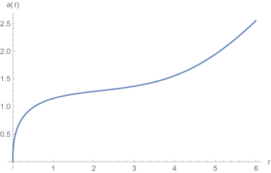
Figure 5: At $k=-1$ and ${2\over\sqrt{e}}<\gamma^{2}$ the value of $\tilde{a}$ is in the interval $\tilde{a}\in[0,\infty]$. The solution shows four stages of alternating expansion. In the first stage there is a period of deceleration, in the second stage the expansion reaches a quasi-stationary evolution near $\tilde{a}\simeq\mu_{c}$, in the third stage there is a period of exponential expansion of a finite duration that undergoes a continuous transition to the fourth stage of a linear in time growth.

The right-hand side of the Friedmann acceleration equation (4) has a similar expression with the Type III solution (116):

$$\epsilon+3p=-8{\cal B}~{}b(\tau)e^{-4b(\tau)-1}\Lambda^{4}_{YM},~{}~{}~{}~{}~{}~{}b\in[-\infty,+\infty],$$ (125)

and the strong energy dominance condition $\epsilon+3p\geq 0$ is violated here when $b>0$ and the region of positive acceleration is wherefore at $b>0$ shown in Fig.6. Thus the deceleration parameter for the Type IV solution is sign alternating, $b\in[-\infty,\infty]$:

$$q_{IV}={b\over b+{1\over 2}(1-{\gamma^{2}\over\gamma^{2}_{c}}e^{2b})},$$ (126)

it is positive for $b\in[-\infty,0)$ and is negative for $b\in(0,\infty]$. Therefore the character of the solution is changing at $b=0$ where the deceleration parameter $q_{IV}=0$. In these two regions the behaviour of the solution is qualitatively different. At the quasi-stationary point $\tau=\tau_{c}$ ($b=0$)

$$\int^{0}_{-\infty}{db~{}e^{2b}\over\Big{(}{\gamma^{2}\over\gamma^{2}_{c}}e^{2b}-1-2b\Big{)}^{1/2}}~{}=\sqrt{{2\over e}}~{}\tau_{c}$$ (127)

we have

$$2g^{2}{\cal F}_{c}={1\over e}\Lambda^{4}_{YM},~{}~{}~{}~{}~{}\epsilon_{c}=-{2{\cal B}\over e}\Lambda^{4}_{YM},~{}~{}~{}~{}~{}p_{c}={2{\cal B}\over 3e}\Lambda^{4}_{YM},$$

and it is reminiscent to the stationary behaviour of the Type III solution (114), (115). The energy density (124) is changing its sign at $\tau=\tau_{0}$ ($b=-1/2$)

$$\int^{-1/2}_{-\infty}{db~{}e^{2b}\over\Big{(}{\gamma^{2}\over\gamma^{2}_{c}}e^{2b}-1-2b\Big{)}^{1/2}}~{}=\sqrt{{2\over e}}~{}\tau_{0}$$ (128)

where we have

$$2g^{2}{\cal F}=e\Lambda^{4}_{YM},~{}~{}~{}~{}~{}\epsilon=0,~{}~{}~{}~{}~{}p={4{\cal B}\over 3e}\Lambda^{4}_{YM}.$$

Figure 6: The r.h.s $\epsilon+3p$ of the Friedmann acceleration equation (4) is positive when $b<0$ and is negative when $b>0$ in the case of Type IV solution (125).

Thus there are four stages of alternating expansions. There is a period of deceleration in the first stage $\tau\ll\tau_{c}$ where $q_{IV}$ is positive. In the second stage, in the vicinity of $\tau\sim\tau_{c}$ where $q_{IV}=0$ the expansion is quasi-stationary and a slow varying scale factor is of order $\tilde{a}(\tau)\simeq\mu_{c}$. In the third stage $\tau>\tau_{c}$ there is a period of exponential expansion of a finite duration $b\sim(0,5)$ where $q_{IV}$ is negative. It is of finite duration because when $b>0$ is large, the acceleration tends to zero:

$$q_{IV}\simeq-{2\over\gamma^{2}\mu^{2}_{c}}be^{-2b}.$$

In the fourth stage $\tau\gg\tau_{c}$, where $e^{b}\simeq{\gamma\over\gamma_{c}}\sqrt{2\over e}\tau$, the acceleration drops to zero $q_{IV}\simeq 0$ and the universe undergoes a continuous transition to a linear in time growth of the scale factor

$$a(t)\simeq~{}ct~{},~{}~{}~{}~{}~{}a(\eta)\simeq~{}e^{\eta}$$ (129)

and the Hubble parameter (49) has the following behaviour:

$$H=\sqrt{{2\over e}}{e^{-2b}\over L}\Big{(}{\gamma^{2}\over\gamma^{2}_{c}}e^{2b}-1-2b\Big{)}^{1/2}\simeq{1\over ct}.$$ (130)

When $\tau\gg\tau_{c}$ the $2g^{2}{\cal F}\rightarrow 0$ and the energy density and pressure are approaching the zero values, $\Omega$ (54) tends to zero value as well:

$$\Omega_{vac}=1-{\gamma^{2}\over({d\tilde{a}\over d\tau})^{2}}=1-{\gamma^{2}e^{2b}\over\gamma^{2}_{c}\Big{(}{\gamma^{2}\over\gamma^{2}_{c}}e^{2b}-1-2b\Big{)}}\rightarrow 0.$$ (131)

The influence of the gauge field theory vacuum on the evolution of the universe is fades out at very late-time. It seems that the Type IV solution is useful to explain a late-time acceleration of the universe expansion if one appropriately adjust the parameters $a_{0}$ and $\gamma$.

10 Flat Geometry, $k=0$

The evolution equation (42) in this case takes the following form:

$${d\tilde{a}\over d\tau}=\pm\sqrt{{1\over\tilde{a}^{2}}\Big{(}\log{{1\over\tilde{a}^{4}}}-1\Big{)}},~{}$$ (132)

and the ”potential” function is (see Fig.7)

$$~{}~{}~{}~{}U_{0}(\tilde{a})\equiv{1\over\tilde{a}^{2}}\Big{(}\log{{1\over\tilde{a}^{4}}}-1\Big{)}.$$ (133)

The solution of the equation $U_{0}(\mu)=0$ determines the values of the scale factor $\tilde{a}=\mu$ at which the square root changes its sign. The evolution equation (132) should be restricted to those real values of $\tilde{a}\in[0,\mu]$ at which the potential $U_{0}(\tilde{a})$ is nonnegative. The maximal value of the scale factor $\tilde{a}_{m}\equiv\mu$ is defined by the equation

$$U_{0}(\mu)={1\over\mu^{2}}\Big{(}\log{{1\over\mu^{4}}}-1\Big{)}=0,~{}~{}~{}~{}\mu^{2}={1\over\sqrt{e}}.$$ (134)

With the substitution

$$\tilde{a}^{4}=\mu^{4}e^{-b^{2}},~{}~{}$$ (135)

where $b\in[-\infty,\infty]$, the equation (132) will take the following form:

$$~{}~{}~{}~{}{db\over d\tau}={2\over\mu^{2}}~{}e^{{b^{2}\over 2}}.$$ (136)

Integrating the equation (136) with the boundary conditions $a(0)=0$, $b(0)=-\infty$ we find

$$\int^{b(\tau)}_{-\infty}dbe^{-{b^{2}\over 2}}={2\over\mu^{2}}~{}\tau,~{}~{}~{}~{}~{}~{}~{}~{}\tau\in[0,2\tau_{m}]$$ (137)

where the half period is

$$\tau_{m}={\mu^{2}\over 2}\int^{0}_{-\infty}dbe^{-{b^{2}\over 2}}=\sqrt{{\pi\over 8e}}.$$ (138)

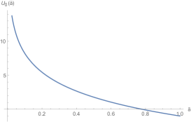
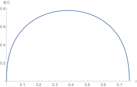
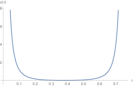
Figure 7: The left figure shows the behaviour of the potential function $U_{0}(\tilde{a})$. It is positive for $\tilde{a}\leq\mu={1\over e^{1/4}}$. The centre figure shows the behaviour of the scale factor $\tilde{a}(\tau)$. The maximal value of the scale factor at the half period  $\tau_{m}=\sqrt{{\pi\over 8e}}$ is $\tilde{a}(\tau_{m})=\mu$. The left figure shows the behaviour of the energy density $\epsilon(\tau)$.

The solution can be expressed in terms of the inverse error function $InverseErf(x)$ [74]

$$b(\tau)=\sqrt{2}InverseErf\Big{(}\sqrt{{8e\over\pi}}~{}(\tau-\tau_{m})\Big{)}$$ (139)

and for $\tilde{a}$ in (135) we will get the solution shown in Fig.7:

$$\tilde{a}(\tau)=\exp{\Big{(}-{1\over 4}-{1\over 2}InverseErf^{2}\Big{(}\sqrt{{8e\over\pi}}~{}(\tau-\tau_{m})\Big{)}\Big{)}}.$$ (140)

The scale factor is periodic in time (140) as it is in closed Friedmann cosmological model (k=1). The asymptotic behaviour of the $\tilde{a}(\tau)$ near $\tau=\tau_{m}$ and $\tau=0$ has the form

$$\tilde{a}(\tau)\simeq\begin{cases}e^{-1/4}-e^{3/4}(\tau-\tau_{m})^{2},~{}~{}~{}~{}~{}\tau\rightarrow\tau_{m}\\ 2\tau^{1/2}\ln^{1/4}{1\over\tau^{1/2}},~{}~{}~{}~{}~{}~{}~{}~{}~{}~{}~{}~{}~{}\tau\rightarrow 0\end{cases},$$ (141)

that is, $\tilde{a}(t)\propto~{}t^{1/2}\ln^{1/4}{1\over t^{1/2}}$. The singularity is logarithmically weaker compared to that in cosmological model with relativistic matter where $\tilde{a}(t)\propto~{}t^{1/2}$. For the field strength we have (46)

$$2g^{2}{\cal F}=e^{b^{2}+1}\Lambda^{4}_{YM}$$ (142)

and for the energy density (135) and pressure (47) evolution in time is

$$\epsilon={\cal B}b^{2}e^{b^{2}+1}\Lambda^{4}_{YM},~{}~{}~{}p={4{\cal B}\over 3}e^{b^{2}+1}\Lambda^{4}_{YM},$$ (143)

where $b(\tau)$ is given in (139) and $\tau=ct/L$. The behaviour of $\epsilon$ is shown in Fig.7. At the half period $\tau=\tau_{m}$ where $\tilde{a}=\tilde{a}_{m}$ ($b=0$) we will have

$$2g^{2}{\cal F}_{m}=e\Lambda^{4}_{YM},~{}~{}~{}~{}~{}\epsilon_{m}=0,~{}~{}~{}~{}~{}~{}~{}~{}p_{m}={4{\cal B}\over 3}~{}e\Lambda^{4}_{YM}.$$ (144)

At the beginning of the expansion from (141) we get

$$2g^{2}{\cal F}\propto{1\over t^{2}\ln{1\over t^{1/2}}},~{}~{}~{}\epsilon\propto{1\over t^{2}\ln{1\over t^{1/2}}}\ln\Big{[}{1\over t^{2}\ln{1\over t^{1/2}}}\Big{]},~{}~{}~{}~{}p\propto{1\over t^{2}\ln{1\over t^{1/2}}}\ln\Big{[}{1\over t^{2}\ln{1\over t^{1/2}}}\Big{]}.$$ (145)

The deceleration parameter (53) here is always positive:

$$q=1+{2\over b^{2}}\geq 1,$$ (146)

where we used (135) and (134). The Hubble parameter and the density parameter $\Omega$ (54) are:

$$H^{2}={\dot{a}^{2}\over a^{2}}={b^{2}\over L^{2}}e^{b^{2}+1},~{}~{}~{}~{}\Omega_{vac}={8\pi G\over 3c^{4}}{\epsilon\over H^{2}}=1.$$ (147)

The expansion proper time interval (43) in this case of flat geometry $k=0$ is (138):

$$~{}~{}~{}~{}~{}ct_{m}=\tau_{m}L=\sqrt{{\pi\over 8e}}L~{}\simeq 4.7\times 10^{24}\Big{(}{eV\over\Lambda_{YM}}\Big{)}^{2}~{}cm,$$ (148)

where $L=1.25\times 10^{25}\Big{(}{eV\over\Lambda_{YM}}\Big{)}^{2}cm$. The physical meaning of this result is that the vacuum energy density $\epsilon$ is able to slow down the expansion earlier than the Hubble time $cH^{-1}_{0}=1.37\times 10^{28}cm$ even in the case of flat geometry ($k=0$). Here the scale $\Lambda_{YM}$ is of order of a few electronvolt $\Lambda_{YM}\sim eV$, as in the case of the Type I solution.

11 Spherical Geometry, $k=1$

The corresponding equation (42) will take the following form:

$${d\tilde{a}\over d\tau}=\pm\sqrt{{1\over\tilde{a}^{2}}\Big{(}\log{{1\over\tilde{a}^{4}}}-1\Big{)}-\gamma^{2}},~{}~{}~{}$$ (149)

and the ”potential” function is

$$U_{+1}(\tilde{a})\equiv{1\over\tilde{a}^{2}}\Big{(}\log{{1\over\tilde{a}^{4}}}-1\Big{)}-\gamma^{2},~{}~{}~{}\text{where}~{}~{}~{}~{}~{}0\leq\gamma^{2}.$$ (150)

The equation $U_{+1}(\tilde{a})=0$ defines the maximal value of the scale factor $\tilde{a}=\mu$ through the equation

$${1\over\mu^{2}}\Big{(}\log{{1\over\mu^{4}}}-1\Big{)}-\gamma^{2}=0.~{}~{}~{}~{}$$ (151)

The substitution

$$\gamma^{2}\mu^{2}=2u$$ (152)

reduces it to the Lamber-Euler equation

$$~{}~{}~{}~{}ue^{u}={\gamma^{2}\over 2\sqrt{e}}.$$ (153)

The solution is expressible in terms of the $W_{0}(x)$ function, which is defined in the positive interval region $0\leq x\leq\infty$:

$$u=W_{0}({\gamma^{2}\over 2\sqrt{e}}),$$ (154)

and it allows to express the maximal value of the scale factor:

$$\mu^{2}={2\over\gamma^{2}}W_{0}({\gamma^{2}\over 2\sqrt{e}})~{}~{}~{}~{}\text{and }~{}~{}~{}~{}0\leq\mu^{2}\leq{1\over\sqrt{e}}.$$ (155)

Thus the scale factor $\tilde{a}$ takes its values in the interval

$$~{}~{}~{}\tilde{a}\in[0,\mu]$$ (156)

shown in Fig.8. With the next substitution

$$\tilde{a}^{4}=\mu^{4}e^{-b^{2}},~{}~{}~{}~{}~{}b\in[-\infty,\infty].$$ (157)

the equation (149) will take the following form:

$${db\over d\tau}={2\over\mu^{2}}~{}e^{{b^{2}\over 2}}\Big{(}1+{\gamma^{2}\mu^{2}\over b^{2}}(1-e^{-{b^{2}\over 2}}\Big{)}^{1/2}.$$ (158)

Integrating the equation with the boundary conditions at $\tau=0$ where $\tilde{a}(0)=0$ and $b(0)=-\infty$ we will get the parametric representation of the function $b(\tau)$:

$$\int^{b(\tau)}_{-\infty}{dbe^{-{b^{2}\over 2}}\over\Big{(}1+{\gamma^{2}\mu^{2}\over b^{2}}(1-e^{-{b^{2}\over 2}}\Big{)}^{1/2}}~{}={2\over\mu^{2}}~{}\tau.$$ (159)

From this equation we obtain $b(\tau)$ by inversion of this elliptic-type integral. The time interval $\tau\in[0,\tau_{m}]$ during which the scale factor is reaching its maximal value (it is equal to a half of the total period, where $b=0$) can be expressed through the integral

$$\int^{0}_{-\infty}{dbe^{-{b^{2}\over 2}}\over\Big{(}1+{\gamma^{2}\mu^{2}\over b^{2}}(1-e^{-{b^{2}\over 2}}\Big{)}^{1/2}}~{}={2\over\mu^{2}}~{}\tau_{m}.$$ (160)

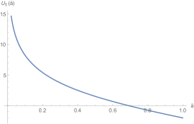
Figure 8: In the case $k=1$ the values of $\tilde{a}$ are in the interval $\tilde{a}\in[0,\mu]$. When $\gamma^{2}=1$, $\mu\simeq 0.69$ and  $\tau_{m}\simeq 0.27$.

The field strength (46) evolution in time is expressible in terms of $b(\tau)$ function:

$$2g^{2}{\cal F}={e^{b^{2}(\tau)}\over\mu^{4}}\Lambda^{4}_{YM}.$$ (161)

The energy density and pressure (47) will evolve in time as well:

$$\epsilon={{\cal B}\over\mu^{4}}e^{b^{2}(\tau)}\Big{(}b^{2}(\tau)+\gamma^{2}\mu^{2}\Big{)}\Lambda^{4}_{YM},~{}~{}~{}~{}~{}~{}~{}~{}~{}~{}p={{\cal B}\over 3\mu^{4}}e^{b^{2}(\tau)}\Big{(}4+b^{2}(\tau)+\gamma^{2}\mu^{2}\Big{)}\Lambda^{4}_{YM}.$$ (162)

The equation of state will take the following form:

$$p={\epsilon\over 3}+~{}{4{\cal B}e^{b^{2}(\tau)}\over 3\mu^{4}}\Lambda^{4}_{YM}.$$ (163)

The equation has an additional term that increases the pressure. The minimal value of the pressure and of the field strength tensor (46) is reached at the midpoint $\tau=\tau_{m}$ where $b(\tau_{m})=0$:

$$2g^{2}{\cal F}_{m}={1\over\mu^{4}}\Lambda^{4}_{YM},~{}~{}~{}~{}~{}~{}\epsilon_{m}={{\cal B}\gamma^{2}\over\mu^{2}}\Lambda^{4}_{YM},~{}~{}~{}~{}~{}p_{m}={\epsilon_{m}\over 3}+{4{\cal B}\over 3\mu^{4}}\Lambda^{4}_{YM}.$$ (164)

The parameter $\mu^{2}$ (155) varies in the interval $0\leq\mu^{2}\leq{1/e^{1/2}}$, therefore $e\Lambda^{4}_{YM}\leq 2g^{2}{\cal F}_{m}$ and $0\leq\epsilon_{m}$. Only the positive part of the energy density curve is involved in the evolution.

Let us consider the limiting behaviour at $\gamma^{2}\rightarrow 0$ and $\gamma^{2}\rightarrow\infty$. In the limit $\gamma^{2}\rightarrow 0$ the solution (159) reduces to the case $k=0$ that was already considered in previous section. In the second limit the maximal value of the scale factor (155) tends to zero $\mu^{2}=\log{\gamma^{2}}/2\gamma^{2}\rightarrow 0$ and the whole universe contracts to the zero size and physical observables are therefore diverging $2g^{2}{\cal F}={\gamma^{4}\over 4\log^{2}{\gamma^{2}}}\rightarrow\infty$, the $\epsilon$ and $p$ are diverging as well. For a typical value of $\gamma^{2}$, let’s say $\gamma^{2}=1$, we have $\mu^{2}=2W_{0}(1/2\sqrt{e})\simeq 0.48$, $\tau_{m}\simeq 0.27$, and the duration of the expansion is:

$$k=1,~{}~{}~{}~{}~{}~{}ct_{m}=\tau_{m}L\simeq 0.27L~{}\simeq 1.12\times 10^{14}\Big{(}{eV\over\Lambda_{YM}}\Big{)}^{2}~{}cm.$$ (165)

Using (151) and (162) for the deceleration parameter (53) one can get:

$$q={b^{2}+\gamma^{2}\mu^{2}+2\over b^{2}+\gamma^{2}\mu^{2}(1-e^{-b^{2}/2})}\geq 1.$$ (166)

There is no acceleration at any time. When $\gamma^{2}\rightarrow 0$ this expression reduces to the $k=0$ expression (146). The Hubble parameter and the density parameter $\Omega$ (54) are:

$$H^{2}={e^{b^{2}}\over L^{2}\mu^{4}}\Big{(}b^{2}+\gamma^{2}\mu^{2}(1-e^{-b^{2}/2})\Big{)},~{}~{}~{}~{}\Omega_{vac}-1={\gamma^{2}\over({d\tilde{a}\over d\tau})^{2}}={\gamma^{2}\mu^{2}e^{-b^{2}/2}\over b^{2}+\gamma^{2}\mu^{2}(1-e^{-b^{2}/2})}.$$ (167)

As one can see, the general behaviour of the solutions in the cases considered in the last two sections: $k=0$, $k=1$ and Type I solution $k=-1$ at $0\leq\gamma^{2}<{2\over\sqrt{e}}$ are qualitatively the same. They all describe a closed universe, as it is shown in Fig.7 for $\tilde{a}(\tau)$. In all these cases the initial value of the scale factor is zero: $a(0)=a_{0}\tilde{a}(0)=0$. The corresponding half-time periods of the expansion are given in (148), (165) and (79).

12 Primordial Gravitational Waves

The coefficient of amplification $K$ of primordial gravitational waves obtained in [29] has the following form:

$$K={1\over 2}\Big{(}{\beta\over n\eta_{0}}\Big{)}^{2},~{}~{}~{}~{}~{}\beta={1-3w\over 1+3w},$$ (168)

where $w$ is the barotropic parameter (5), $n$ is the wave number, the wavelength is $\lambda=2\pi a/n$ and the wave had been initiated at conformal time $\eta_{0}$. A gravitational wave is amplified when equation of state differs from that of radiation ($p={1\over 3}\epsilon$, $w=1/3,~{}\beta=0)$ and earlier this wave had been initiated at $\eta_{0}$. The gravitons are produced with particularly great intensity during the initial exponential expansion of the universe where $\eta_{0}\sim 0$. The production of gravitons is slowing down when the expansion takes a form that is characteristic to the hot universe ($w=1/3$).

In the case of quantum gauge field theory the equation of state has the following form (47):

$$\epsilon={{\cal B}\over\tilde{a}^{4}(t)}\Big{(}\log{{1\over\tilde{a}^{4}(t)}}-1\Big{)}\Lambda^{4}_{YM},~{}~{}~{}~{}~{}~{}~{}p={{\cal B}\over 3\tilde{a}^{4}(t)}\Big{(}\log{{1\over\tilde{a}^{4}(t)}}+3\Big{)}\Lambda^{4}_{YM},$$ (169)

where $a=a_{0}\tilde{a}$ (41) and $a_{0}$ is the initial data parameter (36). The relations between energy density, pressure and the effective parameter $w$ have the following form (48):

$$p={1\over 3}\epsilon+{4\over 3}{{\cal B}\over\tilde{a}^{4}(t)}\Lambda^{4}_{YM},~{}~{}~{}~{}~{}~{}~{}~{}~{}w={p\over\epsilon}={\log{{1\over\tilde{a}^{4}(t)}}+3\over 3\Big{(}\log{{1\over\tilde{a}^{4}(t)}}-1\Big{)}}.$$ (170)

The first relation deviates from $p={1\over 3}\epsilon$ by the additional term depending on the coefficient ${\cal B}$ (34), the scale $\Lambda_{YM}$ and the scale factor $\tilde{a}(t)$. The deviation is large at the initial stages of expansion of the universe and tends to zero at a late time when $\tilde{a}(t)\rightarrow\infty$. Therefore the tensor perturbation of the Type II and Type IV cosmologies naturally amplify the primordial gravitational waves.

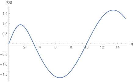
Figure 9: The perturbation of the Type II solution. Here $k=-1$, $\gamma^{2}\simeq 1.211$, $\mu_{2}\simeq 1.32$, the wave number $n=1.01$ and $\tilde{a}(0)=\mu_{2}$, $\theta(0)=0$, $\theta^{{}^{\prime}}(0)=0.1$ in the equations (178) and (179).

The equation describing the tensor perturbation $h_{\mu\nu}$ of the Friedmann space-time metric $\gamma_{\mu\nu}$ is of the form $g_{\mu\nu}=\gamma_{\mu\nu}+h_{\mu\nu}$ and has the following nonzero spacial components:

$$h^{i}_{j}=h(\eta)~{}Y^{i}_{j}~{}e^{inx}={\theta(\eta)\over a(\eta)}~{}Y^{i}_{j}~{}e^{inx},$$ (171)

where $Y^{i}_{j}$ is the tensor eigenfunction of the Laplace operator. In conformal time $\eta$ and t-time the evolution of the linear perturbation has the following form [27]:

$$h^{{}^{\prime\prime}}+2{a^{{}^{\prime}}\over a}h^{{}^{\prime}}+n^{2}h=0,~{}~{}~{}~{}~{}\ddot{h}+3{\dot{a}\over a}\dot{h}+{n^{2}\over a^{2}}h=0,$$ (172)

where $n$ is a wave number and the wavelength is $\lambda=2\pi a/n$. The equation (172) for the $\theta$ amplitude in (171) reduces to the form [29]:

$$\theta^{{}^{\prime\prime}}+\theta(n^{2}-{a^{{}^{\prime\prime}}\over a})=0,$$ (173)

where the derivatives are over conformal time $\eta$ (43), (44). For the general parametrisation of the equation of state $p=w\epsilon$ the solution of Friedmann equations (1) and (3) is:

$$~{}~{}~{}\epsilon\ a^{3(1+w)}=const,~{}~{}~{}~{}~{}~{}a\sim t^{{2\over 3(1+w)}},~{}~{}~{}~{}~{}~{}a\sim\eta^{{2\over 1+3w}}~{}~{}~{}\text{when}~{}~{}~{}k=0.$$ (174)

Considering a universe with a ”break” at $\eta=\eta_{0}$ so that $a(\eta)=const$ and ${a^{{}^{\prime\prime}}\over a}=0$ for $\eta<\eta_{0}$, Grishchuk effectively introduced a potential barrier at $\eta=\eta_{0}$ into the equation (173). Substituting the solution (174) and the ”break” into the (173) one can get [29]

$$\theta^{{}^{\prime\prime}}+\theta\Big{(}n^{2}-\begin{cases}{2(1-3w)\over(1+3w)^{2}}{1\over\eta^{2}},~{}~{}~{}~{}\eta\geq\eta_{0}\\ 0,~{}~{}~{}~{}~{}~{}~{}~{}~{}~{}~{}~{}~{}~{}~{}\eta<\eta_{0}\end{cases}\Bigg{\}}\Big{)}=0.$$ (175)

With the potential barrier in place the amplification of waves (tensor perturbation) takes place when $n\eta_{0}\ll 1$ and the amplification parameter $K$ is given in (168).

Let us now consider the tensor perturbation of Type II solution of the Friedmann equations when the contribution (13) of the gauge field theory vacuum to the energy density of the universe is taken into consideration. For that consider the first first Friedmann equation (44)

$$\Big{(}{\tilde{a}^{{}^{\prime}}\over\tilde{a}}\Big{)}^{2}={1\over\gamma^{2}}{1\over\tilde{a}^{2}}\Big{(}\ln{1\over\tilde{a}^{4}}-1\Big{)}-k$$ (176)

together with the acceleration equation (4), which has the following form:

$${\tilde{a}^{{}^{\prime\prime}}\over\tilde{a}}-\Big{(}{\tilde{a}^{{}^{\prime}}\over\tilde{a}}\Big{)}^{2}=-{1\over\gamma^{2}}{1\over\tilde{a}^{2}}\Big{(}\ln{1\over\tilde{a}^{4}}+1\Big{)}.$$ (177)

Adding together the last two equations gives

$$\tilde{a}^{{}^{\prime\prime}}=-{2\over\gamma^{2}}{1\over\tilde{a}}-k\tilde{a}$$ (178)

and the linear perturbation equation (173) will take the form

$$\theta^{{}^{\prime\prime}}+\theta\Big{(}n^{2}+{2\over\gamma^{2}}{1\over\tilde{a}^{2}}+k\Big{)}=0.$$ (179)

In the case of the Type II solution where $\tilde{a}(0)=\mu_{2}$ (82) the system avoids a singular behaviour in vicinity of $\eta=0$. The amplification of the primordial gravitational waves is due to the second term in (179) when $n^{2}<{2/\gamma^{2}\mu^{2}_{2}}$. The Fig.9 shows the behaviour of the linear perturbation of the Type II solution. The analysis of the system of equations (178) and (179) in details will be published elsewhere.

13 Acknowledgement

I would like to thank Viatcheslav Mukhanov and Dieter Lüst for the invitation to the Sommerfeld Theory Colloquium on the physics of the QCD vacuum [120], the kind hospitality at the LMU of Munich and the discussions that reiterate my interest to physics of the neutron stars [121], gravity [122] and inflationary cosmology. It is a pleasure to express my thanks to Luis Alvarez-Gaume for kind hospitality at the Simons Centre for Geometry and Physics where part of this calculation was initiated. This work was partially supported by the Science Committee of the Republic of Armenia, the research project No. 20TTWS-1C035.

14 Appendix A

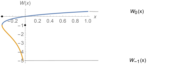
Figure 10: The graph of W-function with its two real branches $W_{0}(x)$ and $W_{-1}(x)$. The two branches merge at the point $(-1/e,-1)$.

The Lambert-Euler W-function $W(x)$ is the solution of the equation [71, 72, 73]:

$$We^{W}=x.$$ (180)

There are two real branches of $W(x)$ (see Fig.10). The solution for which $-1\leq W(x)$ is the principal branch and denoted as $W_{0}(x)$. The solution satisfying $W(x)\leq-1$ is denoted by $W_{-1}(x)$. On the x-interval $[0,\infty)$ there is one real solution, and it is nonnegative and increasing. On the x-interval $[-1/e,0)$ there are two real solutions, one increasing and the other one decreasing. Properties include:

$$W_{0}(-1/e)=W_{-1}(-1/e)=-1,~{}~{}~{}W_{0}(0)=0,~{}~{}~{}W_{0}(e)=1,,~{}~{}~{}W_{0}(e^{1+e})=e,$$ (181)

$$W_{0}(x)=\sum^{\infty}_{n=1}{(-n)^{n-1}\over n!}x^{n}=x-x^{2}+{3\over 2}x^{3}...,~{}~{}~{}|x|<1/e,~{}~{}~{}~{}~{}$$

$$W_{0}(x)=\log x-\log\log x+{\cal O}\Big{(}{\log\log x\over\log x}\Big{)},~{}~{}~{}x\rightarrow+\infty$$

$$W_{-1}(x)=-\log(-{1\over x})-\log\log(-{1\over x})+{\cal O}\Big{(}{\log\log(-{1\over x})\over\log(-{1\over x})}\Big{)},~{}~{}~{}x\rightarrow-0$$

References

- [1] Y. B. Zel’dovich, The Cosmological constant and the theory of elementary particles, Sov. Phys. Usp. 11 (1968) 381 [Usp. Fiz. Nauk 95 (1968) 209]. http://dx.doi.org/10.1070/PU1968v011n03ABEH003927; JETP Lett. 6 (1967) 316
- [2] S. Weinberg, The Cosmological constant problem, Rev. Mod. Phys. 61 (1989) 1-23
- [3] G. Savvidy, Gauge field theory vacuum and cosmological inflation without scalar field, Annals Phys. 436 (2022), 168681 doi:10.1016/j.aop.2021.168681 [arXiv:2109.02162 [hep-th]].
- [4] G. K. Savvidy, Infrared Instability of the Vacuum State of Gauge Theories and Asymptotic Freedom, Phys. Lett. 71B (1977) 133. doi:10.1016/0370-2693(77)90759-6
- [5] G. Savvidy, From Heisenberg–Euler Lagrangian to the discovery of Chromomagnetic Gluon Condensation, Eur. Phys. J. C 80 (2020) 165; doi:10.1140/epjc/s10052-020-7711-6 [arXiv:1910.00654 [hep-th]].
-
[6]
G. K. Savvidy,
Vacuum Polarisation by Intensive Gauge Fields, PhD 1977,
http://www.inp.demokritos.gr/~savvidy/phd.pdf - [7] I. A. Batalin, S. G. Matinyan and G. K. Savvidy, Vacuum Polarization by a Source-Free Gauge Field, Sov. J. Nucl. Phys. 26 (1977) 214 [Yad. Fiz. 26 (1977) 407].
- [8] S. G. Matinyan and G. K. Savvidy, Vacuum Polarization Induced by the Intense Gauge Field, Nucl. Phys. B 134 (1978) 539. doi:10.1016/0550-3213(78)90463-7
- [9] G. Savvidy, Stability of Yang Mills Vacuum State, [arXiv:2203.14656 [hep-th]].
- [10] A. Friedman, On the Curvature of Space , General Relativity and Gravitation 31 (1999) 1991; Über die Krümmung des Raumes Zeitschrift für Physik 10 (1922) 377-386
- [11] A. Friedman, On the Possibility of a World with Constant Negative Curvature of Space, General Relativity and Gravitation 31 (1999) 2001; Über die Möglichkeit einer Welt mit konstanter negativer Krümmung des Raumes 21 (1924) 326-332
- [12] A. A. Starobinsky, A New Type of Isotropic Cosmological Models Without Singularity, Phys. Lett. B 91 (1980), 99-102 doi:10.1016/0370-2693(80)90670-X
- [13] A. H. Guth, The Inflationary Universe: A Possible Solution to the Horizon and Flatness Problems, Phys. Rev. D 23 (1981), 347-356 doi:10.1103/PhysRevD.23.347
- [14] V. F. Mukhanov and G. V. Chibisov, Quantum Fluctuations and a Nonsingular Universe, JETP Lett. 33 (1981), 532-535
- [15] A. H. Guth and S. Y. Pi, Fluctuations in the New Inflationary Universe, Phys. Rev. Lett. 49 (1982), 1110-1113 doi:10.1103/PhysRevLett.49.1110
- [16] V. Mukhanov, Physical Foundations of Cosmology, (Cambridge University Press, New York, 2005).
- [17] T. S. Bunch and P. C. W. Davies, Quantum Field Theory in de Sitter Space: Renormalization by Point Splitting, Proc. Roy. Soc. Lond. A 360 (1978), 117-134 doi:10.1098/rspa.1978.0060
- [18] A. D. Linde, Inflationary Cosmology, Lect. Notes Phys. 738 (2008), 1-54 doi:10.1007/978-3-540-74353-8_1 [arXiv:0705.0164 [hep-th]].
- [19] A. Linde, A brief history of the multiverse, Rept. Prog. Phys. 80 (2017) no.2, 022001 doi:10.1088/1361-6633/aa50e4
- [20] F. L. Bezrukov and M. Shaposhnikov, The Standard Model Higgs boson as the inflaton, Phys. Lett. B 659 (2008), 703-706 doi:10.1016/j.physletb.2007.11.072 [arXiv:0710.3755 [hep-th]].
- [21] R. Kallosh and A. Linde, Superconformal generalizations of the Starobinsky model, JCAP 06 (2013), 028 doi:10.1088/1475-7516/2013/06/028
- [22] P. G. Ferreira, C. T. Hill, J. Noller and G. G. Ross, /Higgs inflation and the hierarchy problem, [arXiv:2108.06095 [hep-ph]].
- [23] I. Antoniadis, A. Guillen and K. Tamvakis, Ultraviolet behaviour of Higgs inflation models, JHEP 08 (2021), 018 doi:10.1007/JHEP08(2021)018 [arXiv:2106.09390 [hep-th]].
- [24] J. L. Cervantes-Cota and H. Dehnen, Induced gravity inflation in the standard model of particle physics, Nucl. Phys. B 442 (1995), 391-412 doi:10.1016/0550-3213(95)00128-X
- [25] R. M. Wald, General Relativity, (University of Chicago Press, Chicago, 1984)
- [26] A. Liddle, An Introduction to Modern Cosmology, (Wiley, West Sussex, 2003).
- [27] E. Lifshitz, Republication of: On the gravitational stability of the expanding universe, J. Phys. (USSR) 10 (1946) 116, doi:10.1007/s10714-016-2165-8
- [28] L. D. Landau and E. M. Lifshitz, The Classical Theory of Fields, (Elsevier, Amsterdam, 1997).
-
[29]
L. P. Grishchuk,
Amplification of gravitational waves in an isotropic universe,
Zh. Eksp. Teor. Fiz. 67 (1974) 825-838; [Sov. Phys. JETP 40 (1975) 409];
L. P. Grishchuk, Graviton creation in the early universe , Ann. NY Acad. Sci. 302 (1977) 439, https://doi.org/10.1111/j.1749-6632.1977.tb37064.x - [30] L. P. Grishchuk, Primordial gravitons and possibility of their observation, Piśma Zh. Eksp. Teor. Fiz. 23 (1976) 326 [JETP Lett. 23 (1976) 293]
- [31] A. A. Starobinsky, Spectrum of relict gravitational radiation and early state of the universe, Piśma Zh. Eksp. Teor. Fiz. 30 (1979) 719 (1979) [JETP Lett. 30 (1979) 683 ]
- [32] V. A. Rubakov, M. V. Sazhin and A. V. Veryaskin, Graviton Creation in the Inflationary Universe and the Grand Unification Scale, Phys. Lett. B 115 (1982), 189-192, doi:10.1016/0370-2693(82)90641-4
- [33] P. J. E. Peebles and A. Vilenkin, Quintessential inflation, Phys. Rev. D 59 (1999), 063505; doi:10.1103/PhysRevD.59.063505 [arXiv:astro-ph/9810509 [astro-ph]].
- [34] S. L. Adler, Einstein Gravity as a Symmetry-Breaking Effect in Quantum Field Theory, Rev. Mod. Phys. 54 (1982) 729; doi:10.1103/RevModPhys.54.729
- [35] J. F. Donoghue, Cosmological constant and the use of cutoffs, Phys. Rev. D 104 (2021) no.4, 045005 doi:10.1103/PhysRevD.104.045005
- [36] E. K. Akhmedov, Vacuum energy and relativistic invariance, [arXiv:hep-th/0204048 [hep-th]].
- [37] G. Ossola and A. Sirlin, Considerations concerning the contributions of fundamental particles to the vacuum energy density, Eur. Phys. J. C 31 (2003), 165-175 doi:10.1140/epjc/s2003-01337-7
- [38] E. S. Fradkin and G. A. Vilkovisky, S matrix for gravitational field. ii. local measure, general relations, elements of renormalization theory, Phys. Rev. D 8 (1973), 4241-4285 doi:10.1103/PhysRevD.8.4241
- [39] R. Pasechnik, G. Prokhorov and O. Teryaev, Mirror QCD and Cosmological Constant, Universe 3 (2017) no.2, 43 doi:10.3390/universe3020043 [arXiv:1609.09249 [hep-ph]].
- [40] W. Heisenberg and H. Euler, Consequences of Dirac’s theory of positrons, Z. Phys. 98 (1936) 714.
- [41] H. Euler and B. Kockel, Über die Streuung von Licht an Licht nach der Diracschen Theorie, Naturwiss. 23 (1935) 246.
- [42] J. S. Schwinger, On gauge invariance and vacuum polarization, Phys. Rev. 82 (1951) 664. doi:10.1103/PhysRev.82.664
- [43] S. R. Coleman and E. J. Weinberg, Radiative Corrections as the Origin of Spontaneous Symmetry Breaking, Phys. Rev. D 7 (1973) 1888. doi:10.1103/PhysRevD.7.1888
- [44] V. S. Vanyashin and M. V. Terentev, The Vacuum Polarization of a Charged Vector Field, Zh. Eksp. Teor. Fiz. 48 (1965) no.2, 565 [Sov. Phys. JETP 21 (1965) no.2, 375].
- [45] V. V. Skalozub, The Vacuum Polarization of the Charged Vector Field in the Renormalized Theory, Yad. Fiz. 21 (1975) 1337.
- [46] M. R. Brown and M. J. Duff, Exact Results for Effective Lagrangians, Phys. Rev. D 11 (1975) 2124. doi:10.1103/PhysRevD.11.2124
- [47] M. J. Duff and M. Ramon-Medrano, On the Effective Lagrangian for the Yang-Mills Field, Phys. Rev. D 12 (1975) 3357. doi:10.1103/PhysRevD.12.3357
- [48] N. K. Nielsen and P. Olesen, An Unstable Yang-Mills Field Mode, Nucl. Phys. B 144 (1978) 376. doi:10.1016/0550-3213(78)90377-2
- [49] V. V. Skalozub, On Restoration of Spontaneously Broken Symmetry in Magnetic Field, Yad. Fiz. 28 (1978) 228.
- [50] H. B. Nielsen, Approximate QCD Lower Bound for the Bag Constant , Phys. Lett. 80B (1978) 133. doi:10.1016/0370-2693(78)90326-X
- [51] J. Ambjorn, N. K. Nielsen and P. Olesen, A Hidden Higgs Lagrangian in QCD, Nucl. Phys. B 152 (1979) 75. doi:10.1016/0550-3213(79)90080-4
- [52] H. B. Nielsen and M. Ninomiya, A Bound on Bag Constant and Nielsen-Olesen Unstable Mode in QCD, Nucl. Phys. B 156 (1979) 1. doi:10.1016/0550-3213(79)90490-5
- [53] H. B. Nielsen and P. Olesen, A Quantum Liquid Model for the QCD Vacuum: Gauge and Rotational Invariance of Domained and Quantized Homogeneous Color Fields, Nucl. Phys. B 160 (1979) 380. doi:10.1016/0550-3213(79)90065-8
- [54] H. B. Nielsen and M. Ninomiya, Instanton Correction to Some Vacuum Energy Densities and the Bag Constant, Nucl. Phys. B 163 (1980) 57. doi:10.1016/0550-3213(80)90390-9
- [55] H. B. Nielsen and P. Olesen, Quark Confinement In A Random Color Magnetic Ether, NBI-HE-79-45.
- [56] J. Ambjorn and P. Olesen, On the Formation of a Random Color Magnetic Quantum Liquid in QCD, Nucl. Phys. B 170 (1980) 60. doi:10.1016/0550-3213(80)90476-9
- [57] J. Ambjorn and P. Olesen, A Color Magnetic Vortex Condensate in QCD, Nucl. Phys. B 170 (1980) 265. doi:10.1016/0550-3213(80)90150-9
- [58] V. V. Skalozub, Nonabelian Gauge Theories In External Electromagnetic Field. (in Russian), Yad. Fiz. 31 (1980) 798.
- [59] H. Leutwyler, Vacuum Fluctuations Surrounding Soft Gluon Fields, Phys. Lett. 96B (1980) 154. doi:10.1016/0370-2693(80)90234-8
- [60] H. Leutwyler, Constant Gauge Fields and their Quantum Fluctuations, Nucl. Phys. B 179 (1981) 129. doi:10.1016/0550-3213(81)90252-2
- [61] M. J. Duff, Observations on Conformal Anomalies, Nucl. Phys. B 125 (1977) 334. doi:10.1016/0550-3213(77)90410-2
- [62] D. Kay, R. Parthasarathy and K. S. Viswanathan Constant self-dual Abelian gauge fields and fermions in SU(2) gauge theory, Phys. Phys. D 28 (1983) 3116-3120.
- [63] W. Dittrich and M. Reuter, Effective QCD Lagrangian With Zeta Function Regularization, Phys. Lett. 128B (1983) 321. doi:10.1016/0370-2693(83)90268-X
- [64] D. Zwanziger, Nonperturbative Modification of the Faddeev-popov Formula and Banishment of the Naive Vacuum, Nucl. Phys. B 209 (1982) 336. doi:10.1016/0550-3213(82)90260-7
- [65] C. A. Flory, Covariant Constant Chromomagnetic Fields And Elimination Of The One Loop Instabilities, Preprint, SLAC-PUB-3244, http://www-public.slac.stanford.edu/sciDoc/docMeta.aspx?slacPubNumber=SLAC-PUB-3244
- [66] H. Pagels and E. Tomboulis, Vacuum of the Quantum Yang-Mills Theory and Magnetostatics, Nucl. Phys. B 143 (1978) 485. doi:10.1016/0550-3213(78)90065-2
- [67] S. Mandelstam, Approximation Scheme for QCD, Phys. Rev. D 20 (1979) 3223. doi:10.1103/PhysRevD.20.3223
- [68] T. R. Taylor and G. Veneziano, Strings and D=4, Phys. Lett. B 212 (1988) 147. doi:10.1016/0370-2693(88)90515-1
- [69] M. Reuter and C. Wetterich, Search for the QCD ground state, Phys. Lett. B 334 (1994) 412 doi:10.1016/0370-2693(94)90707-2 [hep-ph/9405300].
- [70] G. Savvidy, Asymptotic freedom of non-Abelian tensor gauge fields, Phys. Lett. B 732 (2014), 150-155 doi:10.1016/j.physletb.2014.03.022
- [71] J. H. Lambert, Observationes variae in mathesin puram, Acta Helvetica, physico-mathematico-anatomico-botanico-medica 3, Basel (1758) 128-168.
-
[72]
L. Euler, De serie Lambertina plurimisque eius insignibus proprietatibus.
Leonhardi Euleri Opera Omnia, Ser. 1, Opera Mathematica 6 (1921) (original 1779) 350-369. - [73] R. M. Corless, G. H. Gonnet, D. E. G. Hare, D. J. Jeffrey and D. E. Knuth On the Lambert W function, Advances in Computational Mathematics 5 (1996) 329-359.
- [74] M. Abramowitz and I. A. Stegun, (Eds.). Error Function and Fresnel Integrals. Ch. 7 in Handbook of Mathematical Functions with Formulas, Graphs, and Mathematical Tables, 9th printing. New York: Dover, pp. 297-309, 1972
- [75] G. Baseyan, S. Matinyan and G. Savvidy, Nonlinear plane waves in the massless Yang-Mills theory, Pisma Zh. Eksp. Teor. Fiz. 29 (1979) 641-644
- [76] S. Matinyan, G. Savvidy and N. Ter-Arutyunyan-Savvidi, Classical Yang-Mills mechanics. Nonlinear colour oscillations, Zh. Eksp. Teor. Fiz. 80 (1980) 830-838
- [77] G. M. Asatrian and G. K. Savvidy, Configuration Manifold of Yang-Mills Classical Mechanics, Phys. Lett. A 99 (1983), 290 doi:10.1016/0375-9601(83)90887-3
- [78] G. K. Savvidy, Classical and Quantum Mechanics of Non-Abelian Gauge Fields, Nucl. Phys. B 246 (1984) 302. doi:10.1016/0550-3213(84)90298-0
- [79] G. Savvidy, The Yang-Mills classical mechanics as a Kolmogorov system, Phys. Lett. 130B (1983) 303-307
- [80] G. K. Savvidy, Yang-Mills Quantum Mechanics, Phys. Lett. 159B (1985) 325. doi:10.1016/0370-2693(85)90260-6
- [81] J. Hoppe, MIT Ph.D. Thesis, (1982).
- [82] B.V. Chirikov, D.L. Shepelyansky, Stochastic oscillation of classical Yang-Mills fields, JETP Lett. 34 (1981) 163.
- [83] L. Ermann and D. L. Shepelyansky, Deconfinement of classical Yang-Mills color fields in a disorder potential, Chaos 31 (2021), 093106 doi:10.1063/5.0057969 [arXiv:2103.16621 [cond-mat.str-el]].
- [84] E.S. Nikolaevsky, L.N. Shchur, Nonintegrability of the classical Yang-Mills fields, JETP Lett. 36 (1982) 218.
- [85] B. de Wit, M. Luscher, H. Nicolai, The supermembrane is unstable, Nucl. Phys. B 320 (1989) 135.
- [86] T. Banks, W. Fischler, S. H. Shenker and L. Susskind, M theory as a matrix model: A Conjecture, Phys. Rev. D 55 (1997), 5112-5128 doi:10.1103/PhysRevD.55.5112 [arXiv:hep-th/9610043 [hep-th]].
- [87] N. Acharyya, A. P. Balachandran, M. Pandey, S. Sanyal and S. Vaidya, Glueball spectra from a matrix model of pure Yang–Mills theory, Int. J. Mod. Phys. A 33 (2018) no.13, 1850073 doi:10.1142/S0217751X18500732 [arXiv:1606.08711 [hep-th]].
- [88] A. P. Balachandran, S. Vaidya and A. R. de Queiroz, A Matrix Model for QCD, Mod. Phys. Lett. A 30 (2015) no.16, 1550080 doi:10.1142/S0217732315500807 [arXiv:1412.7900 [hep-th]].
- [89] H. P. Pavel, Low-energy spectrum of SU(3) Yang-Mills Quantum Mechanics, [arXiv:2112.06248 [hep-th]].
- [90] J. Ambjorn, K. N. Anagnostopoulos, W. Bietenholz, T. Hotta and J. Nishimura, Monte Carlo studies of the IIB matrix model at large N, JHEP 07 (2000), 011 doi:10.1088/1126-6708/2000/07/011 [arXiv:hep-th/0005147 [hep-th]].
- [91] J. Ambjorn, K. N. Anagnostopoulos, W. Bietenholz, T. Hotta and J. Nishimura, Large N dynamics of dimensionally reduced 4-D SU(N) superYang-Mills theory, JHEP 07 (2000), 013 doi:10.1088/1126-6708/2000/07/013 [arXiv:hep-th/0003208 [hep-th]].
- [92] J. Maldacena, S. H. Shenker and D. Stanford, A bound on chaos, JHEP 1608 (2016) 106 doi:10.1007/JHEP08(2016)106 [arXiv:1503.01409 [hep-th]].
- [93] G. Gur-Ari, M. Hanada and S. H. Shenker, Chaos in Classical D0-Brane Mechanics, JHEP 1602 (2016) 091 doi:10.1007/JHEP02(2016)091 [arXiv:1512.00019 [hep-th]].
- [94] J. S. Cotler et al., Black Holes and Random Matrices, JHEP 1705 (2017) 118 Erratum: [JHEP 1809 (2018) 002] doi:10.1007/JHEP09(2018)002, 10.1007/JHEP05(2017)118 [arXiv:1611.04650 [hep-th]].
- [95] I. Y. Aref’eva, A. S. Koshelev and P. B. Medvedev, Chaos order transition in Matrix theory, Mod. Phys. Lett. A 13 (1998) 2481, [hep-th/9804021].
- [96] I. Y. Aref’eva, P. B. Medvedev, O. A. Rytchkov and I. V. Volovich, Chaos in M(atrix) theory, Chaos Solitons Fractals 10 (1999) 213, [hep-th/9710032].
- [97] I. Y. Aref’eva, A. S. Koshelev and P. B. Medvedev, On stable sector in supermembrane matrix model, Nucl. Phys. B 579 (2000) 411 doi:10.1016/S0550-3213(00)00205-4 [hep-th/9911149].
- [98] I. Y. Aref’eva and I. V. Volovich, Holographic thermalization, Theor. Math. Phys. 174 (2013) 186 [Teor. Mat. Fiz. 174 (2013) 216]. doi:10.1007/s11232-013-0016-2
- [99] O. Fukushima and K. Yoshida, Chaotic instability in the BFSS matrix model, [arXiv:2204.06391 [hep-th]].
- [100] A. Golovnev, V. Mukhanov and V. Vanchurin, Vector Inflation, JCAP 06 (2008), 009 doi:10.1088/1475-7516/2008/06/009 [arXiv:0802.2068 [astro-ph]].
- [101] A. Golovnev, V. Mukhanov and V. Vanchurin, Gravitational waves in vector inflation, JCAP 11 (2008), 018 doi:10.1088/1475-7516/2008/11/018 [arXiv:0810.4304 [astro-ph]].
- [102] A. Maleknejad and M. M. Sheikh-Jabbari, Non-Abelian Gauge Field Inflation, Phys. Rev. D 84 (2011), 043515 doi:10.1103/PhysRevD.84.043515 [arXiv:1102.1932 [hep-ph]].
- [103] E. Elizalde, A. J. Lopez-Revelles, S. D. Odintsov and S. Y. Vernov, Cosmological models with Yang-Mills fields, Phys. Atom. Nucl. 76 (2013), 996-1003 doi:10.1134/S1063778813080097
- [104] E. Elizalde, A. J. Lopez-Revelles, S. D. Odintsov and S. Y. Vernov, Cosmological models with Yang-Mills fields, Phys. Atom. Nucl. 76 (2013), 996-1003 doi:10.1134/S1063778813080097
- [105] P. Adshead and M. Wyman, Gauge-flation trajectories in Chromo-Natural Inflation, Phys. Rev. D 86 (2012), 043530 doi:10.1103/PhysRevD.86.043530 [arXiv:1203.2264 [hep-th]].
- [106] R. Pasechnik, V. Beylin and G. Vereshkov, Possible compensation of the QCD vacuum contribution to the dark energy, Phys. Rev. D 88 (2013) no.2, 023509 doi:10.1103/PhysRevD.88.023509 [arXiv:1302.5934 [gr-qc]].
- [107] R. Pasechnik, Quantum Yang–Mills Dark Energy, Universe 2 (2016) no.1, 4 doi:10.3390/universe2010004 [arXiv:1605.07610 [gr-qc]].
- [108] A. Addazi, T. Lundberg, A. Marcianò, R. Pasechnik and M. Šumbera, Cosmology from Strong Interactions, [arXiv:2204.02950 [hep-ph]].
- [109] J. Cervero and L. Jacobs, Classical Yang-Mills Fields in a Robertson-walker Universe, Phys. Lett. B 78 (1978), 427-429 doi:10.1016/0370-2693(78)90477-X
- [110] L. H. Ford, Inflation Driven by a Vector Field, Phys. Rev. D 40 (1989), 967 doi:10.1103/PhysRevD.40.967
- [111] M. Henneaux, Remarks on Space-Time Symmetries and non-Abelian Gauge Fields, J. Math. Phys. 23 (1982), 830-833 doi:10.1063/1.525434
- [112] Y. Hosotani, Exact Solution to the Einstein Yang-Mills Equation, Phys. Lett. B 147 (1984), 44-46 doi:10.1016/0370-2693(84)90588-4
- [113] D. V. Galtsov and M. S. Volkov, Yang-Mills cosmology: Cold matter for a hot universe, Phys. Lett. B 256 (1991), 17-21 doi:10.1016/0370-2693(91)90211-8
- [114] G. W. Gibbons and A. R. Steif, Yang-Mills cosmologies and collapsing gravitational sphalerons, Phys. Lett. B 320 (1994), 245-252 doi:10.1016/0370-2693(94)90652-1
- [115] A. Golovnev, V. Mukhanov and V. Vanchurin, Vector Inflation, JCAP 06 (2008), 009 doi:10.1088/1475-7516/2008/06/009 [arXiv:0802.2068 [astro-ph]].
- [116] K. Bamba, S. Nojiri and S. D. Odintsov, Inflationary cosmology and the late-time accelerated expansion of the universe in non-minimal Yang-Mills-F(R) gravity and non-minimal vector-F(R) gravity, Phys. Rev. D 77 (2008), 123532 doi:10.1103/PhysRevD.77.123532 [arXiv:0803.3384 [hep-th]].
- [117] A. Maleknejad and M. M. Sheikh-Jabbari, Non-Abelian Gauge Field Inflation, Phys. Rev. D 84 (2011), 043515 doi:10.1103/PhysRevD.84.043515 [arXiv:1102.1932 [hep-ph]].
- [118] E. Elizalde, A. J. Lopez-Revelles, S. D. Odintsov and S. Y. Vernov, Cosmological models with Yang-Mills fields, Phys. Atom. Nucl. 76 (2013), 996-1003 doi:10.1134/S1063778813080097
- [119] P. Adshead and M. Wyman, Gauge-flation trajectories in Chromo-Natural Inflation, Phys. Rev. D 86 (2012), 043530 doi:10.1103/PhysRevD.86.043530 [arXiv:1203.2264 [hep-th]].
- [120] G.Savvidy, Heisenberg-Euler Lagrangian and Discovery of the Magnetic Gluon Condensation, Sommerfeld Theory Colloquium, https://www2.physik.uni-muenchen.de/aus_der_fakultaet/kolloquien/asc_kolloquium/archiv_sose18/savvidy/savvidy.pdf
- [121] D. M. Sedrakian and G. K. Savvidi The form of quantum vortexes in rotating neutron stars. Astrofizika 15 (1979) 359-362; Astrophysics, 15 (1979) 231-233, https://doi.org/10.1007/BF01006047
- [122] V. Gurzadyan and G. Savvidy, Collective relaxation of stellar systems, Astronomy and Astrophysics 160 (1986) 203,