The evolution of high-density cores of the BOSS Great Wall superclusters

Abstract

Context. High-density cores (HDCs) of galaxy superclusters that embed rich clusters and groups of galaxies are the earliest large objects to form in the cosmic web, and the largest objects that may collapse in the present or future.

Aims. We aim to study the dynamical state and possible evolution of the HDCs in the BOSS Great Wall (BGW) superclusters at redshift $z\approx 0.5$ from the CMASS (constant mass) galaxy sample, based on the Baryon Oscillation Spectroscopic Survey (BOSS) in order to understand the growth and evolution of structures in the Universe.

Methods. We analysed the luminosity density distribution in the BGW superclusters to determine the HDCs in them. We derived the density contrast values for the spherical collapse model in a wide range of redshifts and used these values to study the dynamical state and possible evolution of the HDCs of the BGW superclusters. The masses of the HDCs were calculated using stellar masses of galaxies in them. We found the masses and radii of the turnaround and future collapse regions in the HDCs of the BGW superclusters and compared them with those of local superclusters.

Results. We determined eight HDCs in the BGW superclusters. The masses of their turnaround regions are in the range of $M_{\mathrm{T}}\approx 0.4-3.3\times\leavevmode\nobreak\ 10^{15}h^{-1}M_{\odot},$ and radii are in the range of $R_{\mathrm{T}}\approx 3.5-7$ $h^{-1}$ Mpc. The radii of their future collapse regions are in the range of $R_{\mathrm{FC}}\approx 4-8$ $h^{-1}$ Mpc. Distances between individual cores in superclusters are much larger: of the order of $25-35$ $h^{-1}$ Mpc. The richness and sizes of the HDCs are comparable with those of the HDCs of the richest superclusters in the local Universe.

Conclusions. The BGW superclusters will probably evolve to several poorer superclusters with masses similar to those of the local superclusters. This may weaken the tension with the $\Lambda$CDM model, which does not predict a large number of very rich and large superclusters in our local cosmic neighbourhood, and explains why there are no superclusters as elongated as those in the BGW in the local Universe.

1 Introduction

In the complex hierarchical network of galaxies, galaxy groups, clusters, and superclusters, called the cosmic web, the largest systems are galaxy superclusters and supercluster complexes, where several very rich superclusters form chains or planes (as, for example, in the Sloan Great Wall; hereafter SGW) (de Vaucouleurs, 1956; Jõeveer et al., 1978; Einasto et al., 2007a, 2011; Chon et al., 2015; Einasto et al., 2015; Lietzen et al., 2016; Einasto et al., 2016). Rich superclusters embed high-density cores (hereafter HDCs) with one or several rich galaxy clusters, while poor superclusters typically do not have HDCs (Einasto et al., 2007b). The formation of the cosmic web started from tiny density perturbations in the very early Universe (Jõeveer et al., 1978; Kofman & Shandarin, 1988). The skeleton of the cosmic web is fixed by processes during or just after the inflation (Kofman & Shandarin, 1988). The positions of high-density peaks and voids do not change much during the cosmic evolution, only the amplitude of over- and under-densities grows with time (Bond et al., 1996; van de Weygaert & Schaap, 2009; Suhhonenko et al., 2011; Einasto et al., 2019, 2021a, and references therein). Superclusters or their HDCs are the largest systems in the cosmic web that may eventually collapse (de Vaucouleurs, 1956; Jõeveer et al., 1978; Einasto et al., 2015; Chon et al., 2015; Lietzen et al., 2016; Einasto et al., 2016, 2018, 2021b).

Observationally, the studies of protoclusters, progenitors of the present-day galaxy clusters, have shown that they start to form in regions of the highest density in the cosmic density field and are already present at redshifts of $z\approx 6$ (Toshikawa et al., 2016; Overzier, 2016; Lovell et al., 2018, and references therein). Galaxy protoclusters are the first sites of galaxy and cluster formation in a high-redshift universe (Chiang et al., 2017; Marrone et al., 2018; Pavesi et al., 2018; Ando et al., 2020; McConachie et al., 2022). Typically, the most luminous galaxy clusters are located in the HDCs of rich superclusters (Jõeveer et al., 1978).

The advent of deep surveys such as the 2dFRS (2dF Galaxy Redshift Survey), SDSS (Sloan Digital Sky Survey), and CMASS (constant mass) makes it possible to compile supercluster catalogues in a wide redshift interval (Einasto et al., 2007a; Liivamägi et al., 2012; Chow-Martínez et al., 2014) or to determine individual superclusters at high redshifts (Tanaka et al., 2007; Schirmer et al., 2011; Pompei et al., 2016; Kim et al., 2016; Cucciati et al., 2018). To identify elements of the cosmic web, various methods have been used (see e.g. Libeskind et al., 2018, for a review). Superclusters of galaxies have been defined using various methods and criteria, briefly described in Einasto et al. (2020). Superclusters can be defined as the largest connected, relatively isolated objects above a certain density level in the cosmic web (Einasto et al., 1994, 2001; Liivamägi et al., 2012). We also use this definition in the present paper. Luparello et al. (2011) and Chon et al. (2015) defined superclusters as objects that will eventually collapse in the future. Comparison of these definitions shows that the latter definition tends to select HDCs of superclusters obtained using the first definition (Chon et al., 2015; Einasto et al., 2015, 2016). Rich protoclusters, determined at high redshifts, may mark the cores of proto-superclusters (Einasto et al., 2016; Cucciati et al., 2018; Ando et al., 2020; McConachie et al., 2022).

In the $\Lambda$ cold dark matter ($\Lambda$CDM) Universe at redshifts of $z\approx 0.5$ and below, the growth of structures slows down under the influence of the dark energy (Frieman et al., 2008; Einasto et al., 2021a). At this redshift, several superclusters have been discovered (Schirmer et al., 2011; Galametz et al., 2018). We discuss some of them in Sect. 6. Typically, these superclusters resemble local medium-rich superclusters or the HDCs of rich superclusters (Einasto et al., 2018). However, Lietzen et al. (2016) reported a discovery of a very massive extended supercluster complex at redshift of $z=0.45$ named as the BOSS Great Wall (hereafter BGW) using the CMASS sample of the SDSS III (SDSS-III) (Eisenstein et al., 2011; Maraston et al., 2013; Reid et al., 2016). The BGW consists of four superclusters, two of them are extraordinarily rich and more elongated than any local supercluster (Fig. 1 and Einasto et al., 2017). Einasto et al. (2017) analysed the morphology, luminosity, and mass of the BGW superclusters. They found that these superclusters form a complex that is the richest supercluster complex known so far, being richer than the richest supercluster complex in the local Universe, the SGW (Einasto et al., 2016).

Extreme objects such as the BGW usually provide constraints for theories. It is not clear whether systems with sizes, richness, and morphologies similar to those of the BGW can be reproduced in the $\Lambda$CDM model or agree with the Gaussian initial conditions (Einasto et al., 2007c, 2011; Sheth & Diaferio, 2011; Park et al., 2012; Einasto et al., 2017). It is also not clear why there are no such very rich supercluster complexes with very elongated systems in the local Universe. This makes galaxy superclusters and their HDCs at different redshifts unique objects with regard to studies of the formation and evolution of the cosmic web and testing cosmological models and the cosmological principle of homogeneity and isotropy of the Universe. If during the future evolution BGW superclusters break into smaller systems defined by the HDCs of superclusters, similarly to the richest local superclusters such as the Shapley or the Corona Borealis superclusters or the superclusters in the SGW, then the tension with models may weaken or disappear (Chon et al., 2015; Einasto et al., 2016, 2021b).

In this study, our aim is to obtain a better understanding of the evolution of the largest structures in the Universe. We focus on a possible evolution of the BGW superclusters and especially their HDCs. Could it be possible that the BGW superclusters fall apart and form smaller systems during evolution? Answering this question will help to clarify whether the tension with the $\Lambda$CDM model will disappear or weaken. With this aim in mind, we located the HDCs of the BGW superclusters and analysed the possible evolution of their masses and sizes using spherical collapse model. We determined masses of the HDCs of superclusters using stellar masses of high-mass galaxies, as described in detail in Einasto et al. (2017).

For this aim we first needed to derive the parameters of the spherical collapse model for a wide range of redshifts and then apply them to search for possible collapsing regions in the HDCs of the BGW superclusters. We compare the properties of the turnaround and future collapse regions in the HDCs of the BGW superclusters, and in superclusters at different redshifts. Superclusters as a whole are very elongated, but their HDCs are close to spherical, and therefore we can use the spherical collapse model to analyse their dynamical state and possible evolution (Einasto et al., 2021b). We assumed the standard (WMAP) cosmological parameters: the Hubble parameter $H_{0}=100\leavevmode\nobreak\ h$ km s^-1 Mpc^-1, the matter density $\Omega_{\rm m}=0.27$, and the dark energy density $\Omega_{\Lambda}=0.73$ (Komatsu et al., 2011).

2 Data on the BGW superclusters

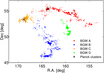
Figure 1: Distribution of galaxies in BGW superclusters in the sky plane. Red dots denote galaxies in BGW A, blue dots in BGW B, yellow dots in BGW C, and green dots in BGW D. Symbol sizes are proportional to the value of the density field at the location of a galaxy. Stars denote the location of Planck clusters.

Table 1: Data on superclusters in BGW.

(1)	(2)	(3)	(4)	(5)	(6)
ID	$N_{\mathrm{gal}}$	Extent	$M$	$M/L$	$D8_{\mathrm{mean}}$
		$h^{-1}$Mpc	$10^{15}h^{-1}M_{\odot}$	$h\,M_{\odot}$/$L_{\odot}$	$\langle\rho_{\mathrm{L}}\rangle$
A	255	186.1	21	277	9.1
B	303	172.9	11	182	9.3
C	73	63.8	7	407	10.2
D	71	90.6	3	118	9.3

To determine galaxy superclusters at redshifts $z\approx 0.5,$ Lietzen et al. (2016) used data from the CMASS galaxy sample based on the Baryon Oscillation Spectroscopic Survey (BOSS; Aihara et al., 2011; Eisenstein et al., 2011; Bolton et al., 2012; Dawson et al., 2013). The CMASS sample includes data about massive and luminous galaxies in the redshift range $0.43<z<0.7$. Their stellar mass is approximately constant up to $z\sim 0.6$ (Maraston et al., 2013). These are galaxies from the high-mass end ($M>10^{11}\leavevmode\nobreak\ M_{\odot}$) of the red-sequence galaxies, which do not evolve over the CMASS redshift range. For details of our sample, we refer the reader to Lietzen et al. (2016).

Galaxy superclusters were determined using the luminosity-density field following the same procedure that was used in Liivamägi et al. (2012). The luminosities of galaxies were weighted to set the mean luminosity density the same through the whole distance range. Then, the luminosity density field was calculated in a 3 $h^{-1}$Mpc grid with an 8 $h^{-1}$Mpc smoothing scale using a $B_{3}$ spline kernel:

$$B_{3}(x)=\frac{1}{12}\left(|x-2|^{3}-4|x-1|^{3}+6|x|^{3}-4|x+1|^{3}+|x+2|^{3}\right).$$ (1)

The calculation of the luminosity-density field is described in detail in Liivamägi et al. (2012).

The BGW superclusters were extracted as connected volumes above the density level $D>6$ times the mean luminosity density of the CMASS sample, $\ell_{\mathrm{mean}}$ = 5$\cdot 10^{-4}$ $\frac{10^{10}h^{-2}L_{\odot}}{(h^{-1}\mathrm{Mpc})^{3}}$) (Lietzen et al., 2016). The BGW supercluster complex consists of two very rich superclusters with maximal extent (the maximal distance between galaxies in the supercluster) 186 $h^{-1}$Mpc (supercluster A) and 173 $h^{-1}$Mpc (supercluster B), and two moderately large superclusters (superclusters C and D) with maximal extent 64 and 91 $h^{-1}$Mpc. Data concerning the BGW superclusters are given in Table 1. In Table 1, the masses are as those derived in Einasto et al. (2017) and explained in Sect. 3.2. Figure 1 presents the sky distribution of galaxies in the BGW superclusters.

Einasto et al. (2017) identified two Planck SZ clusters in the BGW region using data from the Second Planck Catalogue of Sunyaev-Zeldovich Sources (Planck Collaboration et al., 2016): PSZ2 731 in the BGW C and PSZ2 735 in the supercluster BGW A. Their location is shown in Fig. 1.

3 Methods

3.1 Spherical collapse model

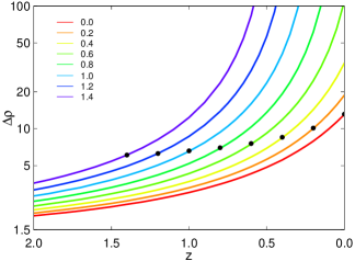
Figure 2: Turnaround density contrast $\Delta\rho_{\mathrm{T}}$ versus redshift at which turnaround occurs, $z_{T}$ (left panel) and evolution of the density contrast $\Delta\rho(t)$ in the spheres, where the turnaround happens at redshifts $z=0.0-1.4$ (right panel). Corresponding redshifts are shown in the figure. Points on each curve show the turnaround density contrast $\Delta\rho_{\mathrm{T}}$ at a corresponding redshift.

The spherical collapse model describes the evolution of a spherical perturbation in an expanding universe. This model was studied, for example, by Peebles (1980), Peebles (1984), and Lahav et al. (1991). In the standard models with cosmological constant, the formation of structures in the cosmic web slows down at redshifts $z\approx 0.5$ due to the influence of the dark energy (Frieman et al., 2008). At the present epoch, the largest bound structures are just forming. During the future evolution these bound systems separate from each other at an accelerating rate, forming isolated ’island universes’ (Chiueh & He, 2002; Dünner et al., 2006; Araya-Melo et al., 2009).

The dynamics of a spherical shell is determined by the mass in its interior. For a spherical volume, the ratio of the density to the mean density (overdensity) $\Delta\rho=\rho/\rho_{\mathrm{m}}$ at different redshifts can be calculated as

$$\Delta\rho=6.88\,\Omega_{\mathrm{m0}}^{-1}\left(\frac{M}{10^{15}h^{-1}M_{\odot}}\right)\left(\frac{R}{5h^{-1}\mathrm{Mpc}}\right)^{-3}\cdot(1+z)^{-3},$$ (2)

where $\Omega_{m0}$ is the matter density parameter at present. From Eq. (2), we can find the mass of a structure as

$$M(R)=1.45\cdot 10^{14}\,\Omega_{\mathrm{m0}}\Delta\rho\left(R/5h^{-1}\mathrm{Mpc}\right)^{3}\cdot(1+z)^{3}h^{-1}M_{\odot}.$$ (3)

The evolution of a spherical shell has several essential epochs, each of which has a characteristic density contrast (Chon et al., 2015; Gramann et al., 2015). These density contrasts can be used to derive the relations between the radius of a perturbation and its interior mass for each essential epoch. In this study, we focused on the turnaround and future collapse. Turnaround is defined as an epoch in the evolution of a spherical perturbation when the sphere stops expanding together with the universe and the collapse begins. Turnaround has a characteristic density contrast which changes with redshift. This means that objects for which the density contrast at a given redshift is not sufficient for the turnaround at this redshift may eventually reach turnaround and experience collapse in the future if their density contrast is high enough (the so-called future collapse).

Next, we briefly describe the evolution of the density contrast. We start with turnaround epoch. The evolution of a density perturbation is affected by the density in it and the spherically averaged radial velocity around it. The spherically averaged radial velocity around a system in the shell of radius $R$ can be written as $u=HR-v_{\mathrm{pec}}$, where $v_{\mathrm{H}}=HR$ is the Hubble expansion velocity and $v_{\mathrm{pec}}$ is the averaged radial peculiar velocity towards the centre of the system. At the turnaround, the peculiar velocity $v_{\mathrm{pec}}=HR$ and $u=0$. The peculiar velocity $v_{\mathrm{pec}}$ is directly related to the overdensity $\Delta\rho$.

As systems evolve, their density increases, and in the standard models with cosmological constant, the density contrast at the turnaround, $\Delta\rho_{T}$, also increases during the evolution. We show this in Fig. 2 for $\Omega_{\mathrm{m0}}=0.27$ and $\Omega_{\mathrm{\Lambda}}=0.73$, which we used in the present study. Figure 2 (left panel) shows how the turnaround density contrast $\Delta\rho_{\mathrm{T}}$ increases with redshift. The overdensity at the turnaround at redshift $z=0.0$ is $\Delta\rho_{\mathrm{T}}=13.1$. The overdensity at the turnaround at the redshift $z=0.5$ (the redshift of the BGW superclusters), $\Delta\rho_{T}=8.0$, and at the redshift $z=1.0$ $\Delta\rho_{T}=6.6$.

The value of the overdensity at the turnaround at a given redshift can be used to calculate the mass of a structure at the turnaround at that redshift. For example, at the redshift $z=0.5,$ the mass of a structure at the turnaround is

$$$$M_{\mathrm{T}}(R)=1.01\cdot 10^{15}\left(R/5h^{-1}\mathrm{Mpc}\right)^{3}h^{-1}M_{\odot}.$$$$ (4)

In addition, in Fig. 2 (right panel) we show the evolution of the density contrast $\Delta\rho(t)$ for cases where the turnaround occurs at a range of redshifts from $z=0.0$ to $z=1.4$. From this figure, one can see, for example, that if the turnaround occurred at redshift $z\approx 0.4$ then the present density contrast for such a structure is $\Delta\rho\approx 30$ (see also Einasto et al., 2020, 2021b, in which this characteristic density contrast around rich clusters in the A2142 and the Corona Borealis superclusters was found).

Another characteristic epoch in the evolution of the density contrast is the future collapse. The superclusters that have not reached the turnaround at a given redshift may eventually turn around and collapse in the future if their density contrast is high enough (Dünner et al., 2006; Chon et al., 2015). These studies showed that the minimum density at redshift $z=0.0$ for a shell to remain bound is $\Delta\rho_{\mathrm{FC}}=8.73$. This corresponds to the turnaround at infinite distant future. At the redshift $z=0.5,$ the overdensity for the collapse at infinite distant future is $\Delta\rho_{\mathrm{FC}}=4.02$, and at the redshift $z=1.0$, the overdensity is $\Delta\rho_{\mathrm{FC}}=2.72$.

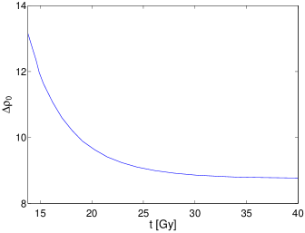
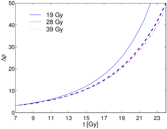
Figure 3: Density contrast $\Delta\rho_{\mathrm{0}}$ at present versus time $t$ at which turnaround occurs (left panel) and evolution of the density contrast $\Delta\rho$ as a function of time $t$ (the age of the Universe) for three different future collapse times ($19$, $28$, and $39$ Gys, right panel).

For intermediate density contrasts $13.1>\Delta\rho>8.73,$ future collapse (turnaround and contraction after that) starts at a certain time in the future. The density contrasts for the collapse at certain times in the future can be calculated by integrating equations for the evolution of a spherical density contrast. We refer the reader to Wang & Steinhardt (1998) and Lee & Ng (2010) for details. We show the density contrast at present as a function of future collapse start time (turnaround time in the future) in the left panel of Fig. 3. The right panel of Fig. 3 shows the evolution of the density contrast as a function of time (the age of the Universe) for three different future collapse times, as given in the figure. The starting time in this figure is approximately $5$ Gyrs past from the present time (this corresponds approximately to the redshift $z=0.5$, which is the redshift of the BGW). Figure 3 shows that at $z=0.5$ ($t\approx 8.8$ Gyrs) density contrasts are $4.4$, $4.09$, and $4.06$, if the collapse occurs in $19$, $28$, or $39$ Gyr. In other words, the density contrast only varies a little.

In our study we used the density contrast for the collapse at infinite distant future, $\Delta\rho_{\mathrm{FC}}=4.02$, to calculate the minimum mass of the structure at the redshift $z=0.5,$ which will turn around and collapse in the future as

$$M_{\mathrm{FC}}(R)=5.29\cdot 10^{14}\left(R/5h^{-1}\mathrm{Mpc}\right)^{3}h^{-1}M_{\odot}.$$ (5)

We used this relation to find the masses and radii of the regions in the HDCs of the BGW superclusters that may eventually collapse during their evolution.

3.2 Determination of masses of HDCs in the BGW superclusters

In the BGW superclusters, only the brightest galaxies can be observed. To determine the mass of the BGW superclusters and their HDCs, we apply the relation between the stellar masses of the first ranked galaxies in haloes, $M_{*}$, and the virial masses of the haloes to which these galaxies belong, $M_{\mathrm{halo}}$ (Moster et al., 2010):

$$\frac{M_{*}}{M_{\mathrm{halo}}}=2\left(\frac{M_{*}}{M_{\mathrm{halo}}}\right)_{0}\left[\left(\frac{M_{\mathrm{halo}}}{M_{1}}\right)^{-\beta}+\left(\frac{M_{\mathrm{halo}}}{M_{1}}\right)^{\gamma}\right]^{-1},$$ (6)

where $(M_{*}/M_{\mathrm{halo}})_{0}=0.0254$ is the normalisation of the stellar-to-halo mass relation, $M_{1}=10^{11.95}$ is a characteristic mass, and $\beta=1.37$ and $\gamma=0.55$ are the slopes of the low and high mass ends of the relation, respectively (Moster et al., 2010, Table 6). The sum of the halo masses gives us an estimate of the lower limit of the supercluster mass. This is the same procedure as was applied in Lietzen et al. (2016) and Einasto et al. (2017) to find the masses of the BGW superclusters.

The stellar masses of BOSS galaxies were obtained from the Portsmouth galaxy product (Maraston et al., 2013), which is based on the stellar population models by Maraston (2005) and Maraston et al. (2009). The Portsmouth product uses an adaptation of the publicly available Hyper-Z code (Bolzonella et al., 2000) to perform a best fit to the observed ugriz magnitudes of BOSS galaxies, with the spectroscopic redshift determined by the BOSS pipeline. The stellar masses used in this work were computed assuming the Kroupa initial mass function.

In calculations of the masses of superclusters, we only used galaxies with stellar masses of $\log(M_{*}/M_{\odot})\geq 11.3$, which is the completeness limit of the CMASS sample (Maraston et al., 2013). We assumed that galaxies in the CMASS sample with $\log(M_{*}/M_{\odot})>11.3$ are the central galaxies of haloes. This is based on comparison with the SDSS main sample of galaxies as follows. We used the magnitude-limited friend-of-friends group catalogue from the SDSS DR10 main sample by Tempel et al. (2014) to select galaxies in superclusters with the luminosity density $D8\geq 5$ in the distance bin from 180 to 270 $h^{-1}$Mpc. From this sample, we determined a BOSS CMASS-like high-mass sample of galaxies with a stellar mass limit of $\log(M_{*}/M_{\odot})\geq 11.3$ and found that 87 % of all galaxies in this high-mass sample are the most luminous, central galaxies in the friend-of-friends groups, or they are single galaxies (the central galaxies of groups with satellite galaxies which are too faint to be observed in the SDSS). Therefore, we can assume that the high-mass galaxies in the BOSS sample are the central galaxies in groups or rich clusters. Comparison with local galaxies suggests that this may introduce an error in mass estimates of the order of about 10–15 %, considering that some massive galaxies may be members of the same group and not the central galaxies of different groups.

There are also haloes whose central galaxies have lower stellar masses than the completeness limit $\log(M_{*}/M_{\odot})=11.3$. To take into account the mass in these haloes, we applied scaling based on the analysis of the SDSS main sample of galaxies. We again used the data concerning galaxies in superclusters with the luminosity density $D8\geq 5$ in the distance bin from 180 to 270 $h^{-1}$Mpc, and found that the ratio between the total stellar mass in high-mass central galaxies and the total stellar mass in all central galaxies in the SDSS superclusters is 0.082. Therefore, we used this ratio to scale our supercluster mass estimates. For details, we refer the reader to Lietzen et al. (2016) and Einasto et al. (2017).

To obtain the total masses of the BGW superclusters, Einasto et al. (2017) used the stellar masses of high-mass galaxies and the scaling as applied here to correct the mass estimate for incompleteness. They additionally used several methods to determine masses of the BGW superclusters and of the SGW in Einasto et al. (2016). In addition to the stellar masses of the central galaxies, they applied mass-to-light ratios and combined morphological and physical parameters of superclusters to determine their masses. Einasto et al. (2017) showed that various methods gave very similar masses of superclusters. For example, the mass of the BGW A supercluster, obtained with different methods, was in the range of $21-23\times\leavevmode\nobreak\ 10^{15}h^{-1}M_{\odot}$, and the mass of the BGW B supercluster in the range of $11-18\times\leavevmode\nobreak\ 10^{15}h^{-1}M_{\odot}$ (Einasto et al., 2017). In the case of SGW those mass estimates that used stellar masses of galaxies gave similar masses as those methods that used dynamical masses of groups. With these methods, Einasto et al. (2016) showed that the total mass of SGW is in the range of $22-24\times\leavevmode\nobreak\ 10^{15}h^{-1}M_{\odot}$. Therefore, different mass estimates are in good agreement, which suggests that we do not have strong biases in the mass estimate of the BGW superclusters; although, we only used data on high-mass galaxies as this sample is complete.

We assume that the high-mass galaxies represent the central galaxies of rich clusters. The number of such clusters in the BGW superclusters is comparable to the number of rich clusters in local rich superclusters such as the superclusters in the SGW or the Corona Borealis supercluster (Einasto et al., 2016, 2021b). However, as we show in Sect. 4.2, with this mass estimate we cannot determine the mass of one possible high-density region in the BGW supercluster that does not contain any high-mass galaxy. Such regions may be similar to, for example, those in the tail of the A2142 supercluster that contain several regions with merging groups (Einasto et al., 2018, 2020).

We find the distribution of mass around the possible centres of the HDCs of the BGW superclusters (see Sect. 4.1). The comparison of the observed mass distribution with the predictions of the spherical collapse model gives us the masses and radii of the turnaround and future collapse regions.

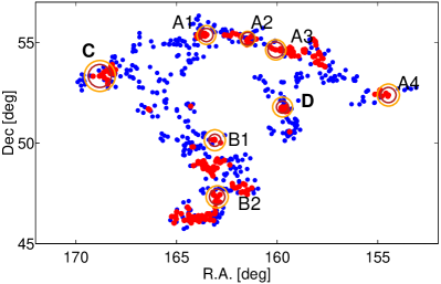
Figure 4: Distribution of galaxies in BGW superclusters in the sky plane. Red dots denote galaxies in the possible HDCs of each supercluster, and blue dots show galaxies in outskirts. Luminosity limits for HDCs are as follows: $D8_{HDC}\geq 15$ in BGW A, $D8_{HDC}\geq 11$ in BGW B, $D8_{HDC}\geq 14.5$ in BGW C, and $D8_{HDC}\geq 16$ in BGW D, where $D8$ is the value of the luminosity density (see text). Dark red circles show the turnaround regions in each HDC, and orange circles show the future collapse regions. Numbers with labels denote HDCs in each BGW supercluster.

For comparison with local superclusters, we also estimated the mass of the HDCs of the BGW superclusters at redshift $z=0.0$. In this comparison, we apply several estimates for the masses and radiii of the collapsing regions. We used the predictions from simulations, which show that the mass of massive haloes increases two times from redshift $z=0.5$ to the present (Kim et al., 2015). We applied this estimate to find the masses of HDCs of superclusters at $z=0.0$ and applied a mass-to-radius relation from the spherical collapse model to estimate radii of cores at this redshift. However, since cores are located in elongated superclusters, this method most probably overestimates the mass. The increase of the mass of supercluster cores can only come from the inflow of mass from the outer parts of a supercluster (see also Tully et al., 2014; Einasto et al., 2019). We can find the mass in the outskirts of superclusters within turnaround radius at $z=0$ using observed mass distribution. Mass estimates of cores obtained in this way are in some cases lower than estimates based on simulations. This is because there is not enough mass in the outer parts of HDCs to increase mass twice as predicted by simulations. We also find masses and radii of the regions in HDCs that may collapse in the future and use them in comparison with local superclusters.

At redshift $z=1.0$ simulations predict that the masses of haloes have approximately five times lower values than their present-day masses (Kim et al., 2015). Using these mass values, we can approximately calculate the sizes of collapsing cores of superclusters at this redshift using their present-day masses (for local superclusters) and masses at redshift $z=0.5$ for the BGW superclusters.

4 HDCs of the BGW superclusters

4.1 Finding HDCs and their turnaround regions in the BGW superclusters

Einasto et al. (2017) analysed the luminosity density field in the BGW superclusters and showed that the HDCs of superclusters can be separated at the density level that includes approximately $1/3$ of supercluster galaxies. At this density level, the characteristic morphology of the superclusters changes. We selected such regions in the BGW superclusters as candidates of the high-density cores of superclusters. Then, we identified high stellar mass galaxies in these regions with stellar masses of $\log(M_{*}/M_{\odot})>11.3$ as the possible main galaxies of groups and clusters. If there was more than one such galaxy, we chose the galaxy with the highest value of the stellar mass as a possible centre of the HDC.

We then drew spheres with an increasing radii around these centre galaxies, and to obtain mass distribution around these centres we calculated masses in the spheres using the stellar masses of galaxies inside them with $\log(M_{*}/M_{\odot})>11.3$. We also corrected for the missing galaxies, as described in Sect. 3.2. Next, we compared the distribution of mass in a core with the distribution of mass obtained from the turnaround and future collapse mass-radius relations as described in Sect. 3.1 (Eqs. 4 and  5). We defined regions that have reached turnaround as regions with radii at which theoretical mass distribution curve and mass distribution from observations crossed. The future collapse regions were defined in the same way, using a mass-radius relation for the future collapse. To be selected as collapsing core of the supercluster, the region has to contain at least two galaxies with stellar mass $\log(M_{*}/M_{\odot})>11.3$ (i.e. there should be at least two possible galaxy groups or clusters; see also Einasto et al., 2021b, who defined massive cores of superclusters as those which have at least two rich clusters).

Data concerning HDCs (their masses, sizes, and richness) are given in Table LABEL:tab:tfc, where masses and radii are given both for turnaround and future collapse regions in HDCs. In this table, we also present estimated masses of the HDC turnaround regions at redshift $z=0$.

4.2 Masses and radii of the collapsing regions in the HDCs

Table 2: Data concerning HDCs in BGW superclusters.

(1)	(2)	(3)	(4)	(5)	(6)	(7)	(8)	(9)	(10)	(11)	(12)	(13)
ID	$\mathrm{R.A.}$	$\mathrm{Dec.}$	$M_{\mathrm{T}}$	$R_{\mathrm{T}}$	$D_{\mathrm{T}}$	$N_{\mathrm{113}}$	$N_{\mathrm{all}}$	$M_{\mathrm{FC}}$	$R_{\mathrm{FC}}$	$M^{\mathrm{est}}_{\mathrm{mod}}$	$R^{\mathrm{est}}_{\mathrm{mod}}$	$M^{\mathrm{est}}_{\mathrm{obs}}$
BGW A
$1$	163.51	55.37	0.96	4.5	16.8	3	21	0.96	6.5	1.9	7.8	1.3
$2$	161.46	55.18	0.35	4.0	15.2	2	8	0.42	4.5	0.8	5.9	0.7
$3$	160.07	54.63	1.8	6.0	10.0	2	22	1.8	7.3	3.6	9.6	1.8
$4$	154.47	52.38	1.6	5.8	16.0	3	8	1.9	7.6	3.2	9.2	1.9
BGW B
$1$	163.10	50.14	0.53	3.5	8.8	2	6	0.9	6.5	1.1	6.4	0.9
$2$	163.00	47.32	0.81	4.5	11.0	2	10	1.6	7.2	1.6	7.3	1.5
BGW C
$1$	168.81	53.33	3.3	7.0	15.0	2	17	3.3	9.5	6.6	11.7	3.3
BGW D
$1$	159.73	51.79	0.42	3.5	11.3	2	11	1.0	6.4	0.8	6.4	1.0

We determined four HDCs in the BGW A supercluster, two in the BGW B supercluster, and one in each of the BGW C and D superclusters. In Fig. 4, we plot the sky distribution of galaxies in the BGW superclusters and show galaxies in HDCs with different colours. The luminosity density limit for HDCs in each supercluster, $D8_{HDC}$, is given in the caption. Figure 4 shows the BGW superclusters as elongated systems, the BGW A and the BGW B superclusters being more elongated than BGW C and BGW D (details about the morphology of the BGW superclusters can be found in Einasto et al., 2017). Data about the HDCs of the BGW superclusters are given in Table LABEL:tab:tfc. Next, we describe HDCs in each BGW supercluster.

The BGW A supercluster has four HDCs. Figure 5 shows the distribution of masses in them. Data on HDCs in BGW A are given in Table LABEL:tab:tfc. Core A1 is centred at the Planck cluster PSZ2 G151.62+54.78 with the mass $M\approx 5.4\times\leavevmode\nobreak\ 10^{14}h^{-1}M_{\odot}$ (Planck Collaboration et al., 2016). Approximately half of the mass here comes from this cluster. Table LABEL:tab:tfc shows that the masses in the turnaround regions of HDCs lie in the range of $M=0.4-1.8\times\leavevmode\nobreak\ 10^{15}h^{-1}M_{\odot}$, and their radii are in the range of $R=4-6$ $h^{-1}$ Mpc. The masses and radii in regions that correspond to the future collapse (calculated for the redshift $z=0.5$) lie in the range of $M=0.4-1.9\times\leavevmode\nobreak\ 10^{15}h^{-1}M_{\odot}$, and $R=4.5-7.6$ $h^{-1}$ Mpc.

The comparison with the total mass of the BGW A supercluster, given in Table 1, shows that turnaround regions of all four HDCs together contain approximately 22% of the total mass of the BGW A supercluster. HDCs themselves contain approximately $1/3$ of the supercluster mass (Sect. 4.1), which means that in some HDCs only the highest density central parts of the cores may collapse during the evolution of the supercluster. The prediction based on simulations (two-times increase of a halo mass) probably overestimates the possible increase of core masses based on mass distribution around haloes at redshift $z=0$ in Table LABEL:tab:tfc. The mass distributions in Fig. 5 show that there are no high-mass clusters at the outskirts of supercluster BGW A, which could join the cores and strongly increase their mass. This agrees with what we know about local superclusters, where rich clusters are preferentially located in the HDCs of superclusters, not in their outskirts (de Filippis et al., 2005; Belsole et al., 2005; Einasto et al., 2020, 2021b). This also suggests that mass estimates for the future collapse that use mass distribution around the centres of HDCs also present a better approximation for the mass at redshift $z=0$. If we compare different mass estimates for the collapsing regions in the HDCs of BGW A in Table LABEL:tab:tfc, then at redshift $z=0$ cores 1 and 2 may have higher masses than predicted by the future collapse.

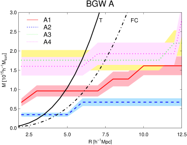
Figure 5: Mass-radius relation for HDCs of BGW supercluster A. Red solid line - A1; blue dashed line - A2; green dashed line - A3; violet dotted line - A4. Black solid and dotted lines show turnaround (T) and future collapse (FC) mass ($M_{\mathrm{T}}(R)$ and $M_{\mathrm{FC}}(R)$) versus radius of a sphere $R$ at redshift $z=0.5$, correspondingly. Dashed areas show 15% mass errors, as explained in the text.

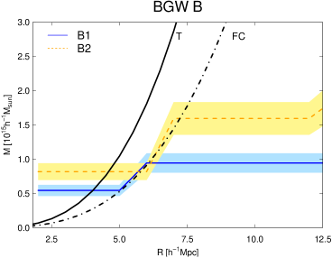
Figure 6: Mass-radius relation for HDCs of BGW supercluster B. Blue solid line - B1; red dashed line - B2.

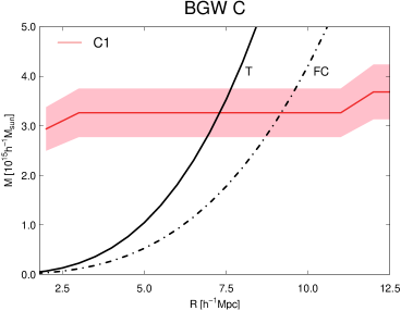
Figure 7: Mass-radius relation for HDC of BGW supercluster C. Red line - C1.

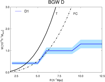
Figure 8: Mass-radius relation for HDC of BGW supercluster D. Blue line - D1.

In the BGW B supercluster, we determined two HDCs. Figure 6 shows the distribution of masses around them. From this figure, we can estimate that the masses of their turnaround regions are $M=0.5\times\leavevmode\nobreak\ 10^{15}h^{-1}M_{\odot}$ and $0.8\times\leavevmode\nobreak\ 10^{15}h^{-1}M_{\odot}$, and their radii are $R=3.5$ $h^{-1}$ Mpc and $R=4.5$ $h^{-1}$ Mpc. In the future, their masses may be twice as high, $M=0.9\times\leavevmode\nobreak\ 10^{15}h^{-1}M_{\odot}$ and $1.6\times\leavevmode\nobreak\ 10^{15}h^{-1}M_{\odot}$, and their radii $R=6.5$ $h^{-1}$ Mpc and $7.2$ $h^{-1}$ Mpc. These values are close to predictions based on observed mass distribution in Table LABEL:tab:tfc. However, Fig. 6 shows that the increase of the mass for the future collapse regions may be smaller, and their masses may stay in the range of $M\approx 0.5-0.9\times\leavevmode\nobreak\ 10^{15}h^{-1}M_{\odot}$ and radii in the range of $R\approx 5-6$ $h^{-1}$ Mpc.

The total mass of the BGW B supercluster is $11\times\leavevmode\nobreak\ 10^{15}h^{-1}M_{\odot}$ (Table 1), therefore the HDCs of the BGW B contain approximately 12% of the total mass of the supercluster at the turnaround. During the future evolution the mass of cores may increase up to approximately $1/4$ of the total mass of the supercluster. Thus, the structure and mass evolution within the BGW B is different from that of BGW A.

We note that in Fig. 4 there is a dense clump of galaxies between HDCs. This clump does not contain any high-mass galaxy with stellar mass $\log(M_{*}/M_{\odot})\geq 11.3$ and thus it is not in the list of HDCs. This clump is similar to, for example, high-density regions in the tail of the local supercluster SCl A2142, which contain several pairs of merging groups. These are collapsing now and may become rich clusters or small superclusters in the future. These structures were described in detail in Einasto et al. (2018) and Einasto et al. (2020).

The highest mass halo in supercluster C can be identified with the Planck cluster PSZ2 G150.56+58.32 with the mass of $M\approx 7.6\times\leavevmode\nobreak\ 10^{14}h^{-1}M_{\odot}$ (Planck Collaboration et al., 2016). Among Planck clusters in the BGW redshift range, $0.47\pm 0.05$, this cluster has the highest estimated mass (Fig. 7). This is also the most massive cluster in the BGW superclusters. The turnaround radius and core mass of the supercluster BGW C are the highest among the HDCs of the BGW superclusters. The mass at the turnaround is $M\approx 3.3\times\leavevmode\nobreak\ 10^{15}h^{-1}M_{\odot}$, which is approximately half of the total mass of the supercluster. The radius of the core of the BGW C is the largest, $R\approx 7.0$ $h^{-1}$ Mpc. Figure 7 shows that in a wide range of radii from the core centre, the mass of the core does not increase, and the mass of the future collapse region is the same as the mass of the turnaround region. The mass in the future collapse region may actually be higher than our estimate, since we cannot directly take into account possible poor groups in the supercluster. However, the size of BGW C is over $60$ $h^{-1}$ Mpc, and we may assume that its outskirts may separate from the collapsing core region in the future.

In BGW D (Fig. 8), the mass and size of the HDC at the turnaround are similar to those of core B2 in BGW B, with a mass of $M\approx 0.4\times\leavevmode\nobreak\ 10^{15}h^{-1}M_{\odot}$, and a radius of $R\approx 3.5$ $h^{-1}$ Mpc. Other rich clusters in BGW D, seen in Fig. 8, may join its highest density core during the evolution, and then its mass will be as high as $M\approx 1.0\times\leavevmode\nobreak\ 10^{15}h^{-1}M_{\odot}$, and its radius $R\approx 6.4$ $h^{-1}$ Mpc. The mass of the core at the turnaround forms approximately 13% of the total supercluster mass and may increase up to approximately $1/3$ of the supercluster mass at the future collapse.

In summary, we found that the masses of turnaround regions of the BGW superclusters are in the range of $M_{T}=0.4-3.3\times\leavevmode\nobreak\ 10^{15}h^{-1}M_{\odot}$. The radii of turnaround regions lie in the range of $R_{T}=3.5-7$ $h^{-1}$ Mpc (Table LABEL:tab:tfc). The masses and sizes of their future collapse regions lie in the same range; however, for three HDCs the masses of the future collapse regions are twice as high as in the turnaround region. Thus, the increase of mass depends on the distribution of structures (galaxy groups and filaments) in the HDCs. At redshift $z=1,$ their masses could have been $M_{T}\approx 0.2-1.6\times\leavevmode\nobreak\ 10^{15}h^{-1}M_{\odot}$, and their sizes are $R_{T}\approx 2.4-4.6$ $h^{-1}$ Mpc (Fig. 10).

4.3 May HDCs merge in the future?

We plot the sky distribution of galaxies from the BGW superclusters in Fig. 4, where we also show the turnaround and future collapse regions of their HDCs. This figure summarises the results of the analysis of the HDCs. FC regions may form separate systems in the future. Before making this conclusion, we intend to check whether different HDCs in the BGW A and B superclusters may still merge in the future. If this is a likely scenario, then they may eventually form very massive and large systems similar to what Einasto et al. (2021b) found for the Corona Borealis supercluster in the local Universe. The answer to this question depends on the quality of our mass estimates of the HDCs, which determine the radii of the turnaround and future collapse regions, and on the mutual distances between HDCs. If HDC masses are high enough to have overlapping core regions at the turnaround, or which may collapse in the future, then they may merge. In Fig. 9, we show the mass-radius relations for the turnaround and future collapse epochs at redshift $z=0.5$ (Eqs. 4 and  5) for radii up to $17.5$ $h^{-1}$ Mpc. From this we can find how large the mass of a core should be in order to be at the turnaround or to collapse in the future, provided we know the radius of a region of interest.

Distances between individual cores in the BGW A (Fig. 5) exceed $25$ $h^{-1}$ Mpc. The sizes of neighbouring future collapse regions in BGW A are much smaller (Table LABEL:tab:tfc). In order to overlap, the sizes of individual future collapse regions in HDCs should be larger than $\approx 13$ $h^{-1}$ Mpc. From Fig. 9, one can see that the mass needed for the future collapse in regions with the radius of $12-15$ $h^{-1}$ Mpc is at least of the order of $10-15\times\leavevmode\nobreak\ 10^{15}h^{-1}M_{\odot}$. This is of the same order as the mass of the full BGW A superclusters, $21-23\times\leavevmode\nobreak\ 10^{15}h^{-1}M_{\odot}$ (Einasto et al., 2017). For the BGW A supercluster, this means that to be that large, even the mass of the most massive core ($1.8\times\leavevmode\nobreak\ 10^{15}h^{-1}M_{\odot}$) must be underestimated by almost ten times its actual value.

Distances between cores of BGW B supercluster (Fig. 6) exceed $30$ $h^{-1}$ Mpc. In order to overlap, each of the HDCs should have masses higher than $15\times\leavevmode\nobreak\ 10^{15}h^{-1}M_{\odot}$ (Fig. 9). This is higher than the total mass of the BGW B supercluster (Table 1), $11-18\times\leavevmode\nobreak\ 10^{15}h^{-1}M_{\odot}$, and six times higher than our estimate for the sum of the masses of the future collapse regions of BGW B.

Figure 9: Mass versus radius for the turnaround (T, red solid line) and future collapse (FC, blue dot-dashed line) at redshift $z=0.5$.

The mass estimates of the BGW superclusters are, of course, more uncertain than the mass estimates of the local superclusters. However, Einasto et al. (2017) determined masses of the BGW superclusters applying several methods, which included a stellar mass-halo mass relation for the first-rank galaxies, as used in this paper, as well as mass-to-light ratios and combined morphological and physical parameters of superclusters to determine supercluster masses. Different mass estimates were in a good agreement (see also Sect. 3.2). Also, mass estimates of the BGW superclusters in Einasto et al. (2017) gave the total mass of the whole BGW $\approx 40-50\times\leavevmode\nobreak\ 10^{15}M_{\odot}$. This is slightly higher than the mass of the most massive superclusters in, for example, Chon et al. (2014), which is expected since the BGW is a complex of four rich superclusters. If the mass of the BGW were ten times higher, then its mass-to-light ratio should also be ten times higher than the value found in Einasto et al. (2017), $M/L\approx 300$ (see Table 1). It is highly unlikely to have $M/L$ for superclusters ten times higher than that. Our mass estimates for the HDCs with Planck clusters agree well with the masses of these clusters (approximately half of the HDC mass comes from the mass of Planck clusters). Therefore, we may assume that the HDCs in BGW A and BGW B never join, and during the evolution BGW A and BGW B will form several separate systems. Of course, we need future studies of superclusters at redshifts around $z=0.5$ to better understand their properties.

5 Comparison with local superclusters

Next, we compare the masses and radii of BGW supercluster HDCs with those of local superclusters (Fig. 10). For this comparison, we used data concerning local superclusters from the supercluster and group catalogues by Liivamägi et al. (2012) and Tempel et al. (2014). These catalogues are based on the MAIN sample of the 8th and 10th data releases of the SDSS (Aihara et al. (2011) and Ahn et al. (2014). To compile group and supercluster catalogues, an apparent Galactic extinction-corrected $r$ magnitude limit $r\leq 17.77$ and redshift limits $0.009\leq z\leq 0.200$ were applied. The redshifts of galaxies were corrected with respect to our motion relative to the CMB and the comoving distances of galaxies were computed, as described in Martínez & Saar (2002) and in Tempel et al. (2014).

Galaxy superclusters were determined as the BGW superclusters using the luminosity density field of galaxies. The calculation of the luminosity density field and determination of superclusters is described in detail in Liivamägi et al. (2012).

To compare the masses and radii of the HDCs in the BGW (at redshift $z=0.5$) and local superclusters (at redshift $z=0$) in Fig. 10, we used data regarding the two richest superclusters in the SGW (Einasto et al., 2016), the Corona Borealis (CorBor) supercluster (Einasto et al., 2021b), and the supercluster SCl A2142 (Einasto et al., 2018). The SGW is a complex of two rich and three poor superclusters. We used data regarding three HDCs in the richest SGW supercluster (denoted as SGW 27) and two cores in the second richest SGW supercluster (SGW 19). In all these studies, the masses and radii of HDCs of superclusters correspond to the masses and radii of the turnaround regions of supercluster cores, they were found using a similar methodology, and therefore we can directly compare their estimates. To compare HDCs at different redshifts, one needs to convert corresponding masses and radii to the same redshift. This is done as described in Sect 3.2.

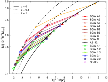
Figure 10: Turnaround mass versus the radius of the turnaround region in the HDCs of superclusters at different redshifts. For each HDC, the turnaround mass and radius are plotted at redshifts $z=0$ (right point), $z=0.5$ (middle point), and $z=1$ (left point). Legend lists HDCs of superclusters plotted in the figure. Black lines show theoretical mass - radius relation for redshifts $z=0.0$ (solid line), $z=0.5$ (dashed line), and $z=1.0$ (dot-dashed line) (Sect. 3.1).

In Fig. 10, we plot the turnaround mass versus radius for the the cores of superclusters at different redshifts. For each supercluster, the turnaround mass and radius are plotted at redshifts $z=0$ (right point), $z=0.5$ (middle point), and $z=1$ (left point). For the BGW supercluster cores, estimated masses and radii at redshift $z=0$ are given using predictions from simulations (Table LABEL:tab:tfc, columns 11 and 12). Black lines in the figure show a theoretical mass - radius relation for redshifts $z=0.0$, $z=0.5$, and $z=1.0$. This figure shows the growth of the supercluster cores that have reached the turnaround and started to collapse.

In Fig. 10, the turnaround region of the HDC of the BGW C supercluster has the highest mass and largest radius at all redshifts. Other turnaround regions of the HDCs of the BGW superclusters are of the same order as turnaround regions in the Corona Borealis and A2142 superclusters. The collapsing cores in the SGW superclusters are less massive.

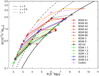
Figure 11: Future collapse mass versus the radius of the HDCs of the BGW superclusters at redshifts $z=0$ (right point; columns 9 and 10 in Table LABEL:tab:tfc), $z=0.5$ (middle point), and $z=1$ (left point), and the masses and radii of the core of the Corona Borealis supercluster and SCl A2142, which at $z=0.5$ correspond to those of their spheres of influence (see text). Legend lists HDCs of superclusters plotted in the figure. Black lines show theoretical mass - radius relation for redshifts $z=0.0$ (solid line), $z=0.5$ (dashed line), and $z=1.0$ (dot-dashed line) (Sect. 3.1).

However, the two-fold increase of the HDC masses of the BGW superclusters in Fig. 10, as predicted in simulations, does not take into account the mass distribution in the HDCs and is probably overestimated for five cores (for BGW A cores, and for BGW C). Also, this prediction is valid for individual haloes, not for HDCs of superclusters analysed in this paper. We argued that the masses and radii of the future collapse regions may also be better indicators for masses and radii of collapsing regions in the BGW superclusters at redshift $z=0$.

For the same reason, the decrease of masses and radii of the cores of local superclusters at high redshifts may be overestimated. We can use another estimate based on the spheres of influence around rich clusters in superclusters. Einasto et al. (2020) and Einasto et al. (2021b) showed that rich clusters in the HDCs of supercluster SCl A2142 and the Corona Borealis are surrounded by a sphere of influence, where all galaxies and groups of galaxies are infalling towards clusters. The masses and sizes of the spheres of influence are of the same order as the masses and sizes of the turnaround regions of the HDCs of the BGW superclusters. The density contrast at the borders of the spheres of influence is $\Delta\rho\approx 30$. Einasto et al. (2020) and Einasto et al. (2021b) found that the spheres of influence passed the turnaround and started to collapse at redshifts $z\approx 0.4$, approximately at the redshift of the BGW. We may assume that the HDCs of the BGW superclusters may be considered the progenitors of the spheres of influence around clusters in the HDCs of local superclusters. Therefore, in Fig. 11 we compare the masses and radii of the future collapse regions of the HDCs of the BGW superclusters (Table LABEL:tab:tfc) and those of the spheres of influence (for SCl A2142 and for the Corona Borealis supercluster; for the SGW cores, we used the same values as in Fig. 10).

As Fig. 11 shows, the differences between the masses and sizes of the BGW superclusters and of other superclusters calculated in this way are smaller than those seen in Fig. 10. Thus, it is possible that the BGW superclusters will evolve to systems similar to the (HDCs of the) local rich superclusters. For example, even BGW C, which has the most massive core among the cores of the BGW superclusters, will probably have a mass close to that of the HDC of the Corona Borealis supercluster (for details, see Einasto et al., 2021b). The HDCs of other BGW superclusters will evolve to systems similar in mass and size to the HDCs of SCL A2142 and of the SGW superclusters.

6 Discussion and summary

6.1 Comparison with other superclusters at redshifts of $z=0.5$ and $z=1$

Are the BGW superclusters typical or exceptional among superclusters at higher redshifts? To answer this question, we briefly compare the BGW superclusters with other superclusters at redshifts of approximately $z=0.5$ and $z=1$.

Schirmer et al. (2011) analysed the mass and structure of supercluster SCl2243 at redshift $z=0.447$. They found that the mass of the central cluster of the supercluster is of the order of $M\approx 1.5\times 10^{15}M_{\odot}$. This is higher than the estimated mass of individual clusters in the BGW (including Planck clusters). The mass of filaments around the central cluster was found to be of the same order. Together, the total mass of SCl2243 is $M\approx 3\times 10^{15}M_{\odot}$, which is of the same order as the total mass of the BGW D supercluster, or as the HDC of the BGW C supercluster. In SCl2243, clusters are connected by several galaxy filaments that are similar in morphology to the BGW C supercluster, described in Einasto et al. (2017).

Verdugo et al. (2012) analysed the galaxy and group content and large-scale structure around a very rich galaxy cluster at redshift $z=0.45$. They found that large-scale structures around the cluster extend up to approximately $20$ Mpc. In this complex, the fraction of blue galaxies decreases with the local density. The galaxy content of groups shows a large variation. They concluded that the large-scale structure around a rich cluster is a dynamical place for galaxy evolution, as also found in the studies of other superclusters (Einasto et al., 2018).

Galametz et al. (2018) discovered a galaxy supercluster at redshift $z=0.65$ and confirmed with VLT/VIMOS spectroscopic observations that it has four galaxy clusters and approximately ten groups. The masses of clusters are of the order of $M\approx 10^{14}M_{\odot}$, which is slightly lower than the masses of Planck clusters in the BGW superclusters. The mass growth of groups in this supercluster from redshift $z=0.65$ to $z=0.46$ (approximately 1.5 times; see Kim et al., 2015) may lead to systems with the same order of mass as the turnaround regions of the HDCs of the BGW superclusters.

Tanaka et al. (2007) found a rich filament of galaxies at redshift $z\approx 0.55$ connecting clumps of galaxies with a massive cluster (with $M\approx 10^{15}M_{\odot}$). These clumps are probably galaxy groups aligned along the filament and probably bound to the main cluster.

Bagchi et al. (2017) reported the discovery of a very rich supercluster at redshift $z\approx 0.3$, which is nicknamed Saraswati. They estimated that the core region within turnaround radius of the Saraswati with very rich Abell cluster A2631 has a mass of $M\approx 4\times 10^{15}M_{\odot}$ and comoving radius of $R\approx 20$ Mpc. The whole Saraswati supercluster is more massive and larger than the Corona Borealis supercluster, which is the most massive among local superclusters used for comparison in this study. Based on the predictions from simulations, we can estimate that the mass of the turnaround region of the Saraswati supercluster at redshift $z\approx 0.5$ could be $M\approx 3\times 10^{15}M_{\odot}$, which is similar to the turnaround region in the BGW C supercluster. There are other similarities between BGW C and Saraswati. There is one very massive galaxy cluster in the cores of both superclusters. The masses of clusters are of the same order, $M\approx 10^{15}M_{\odot}$ (Monteiro-Oliveira et al., 2021). Both of these clusters are also Planck clusters: PSZ2 G150.56+58.32 in BGW C and PSZ2 G087.03-57.37 (A2631) in Saraswati. It could be an interesting future task to compare Saraswati and BGW C in more detail.

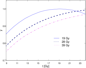
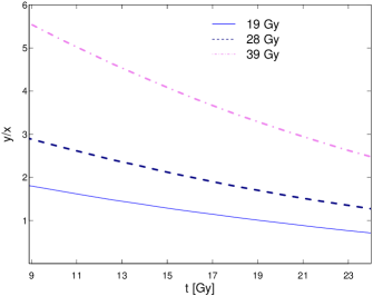
Figure 12: Evolution of radius $R$ of future collapse region with the age of the universe. In the left panel, $y$ denotes the ratio $y=R/R_{T}$, where $R$ is the radius of a overdensity region and $R_{T}$ is its radius at a turnaround time. In the right panel, $x$ denotes the ratio of the usual cosmological scale factor, $a$, to the turnaround scale factor, $a_{T}$ ($x=a/a_{T}$).

The masses of superclusters at redshift $z\approx 0.5$ from these studies are of about $0.1-5\times\leavevmode\nobreak\ 10^{15}M_{\odot}$. A comparison with the masses of HDCs of the BGW superclusters and predicted masses of local superclusters (Table LABEL:tab:tfc and Fig. 10) shows that these masses are of the same order, and we may suppose that superclusters, currently observed at $z\approx 0.5$, will evolve into systems that are of the same size and mass as local rich superclusters or their HDCs.

Kim et al. (2016) reported a discovery of a supercluster at redshift $z\approx 0.9$ that consists of three massive galaxy clusters with separations of approximately $15$ Mpc and masses of the order of $0.1-5\times\leavevmode\nobreak\ 10^{15}M_{\odot}$. This is the same mass range as the estimated masses of superclusters in our study.

Gilbank et al. (2008) and Faloon et al. (2013) analysed a compact supercluster of three massive clusters at redshift $z\approx 0.9$ (RCS 2319+00), with X-ray masses of the order of $\approx 5\times\leavevmode\nobreak\ 10^{14}M_{\odot}$. The authors proposed that these clusters may merge and form a massive cluster at lower redshifts. The mass of clusters is close to our estimate for the cores of the BGW superclusters, and these clusters may represent a structure similar to the HDCs of superclusters.

One of the largest superclusters discovered at redshift $z\approx 0.9$ is the supercluster CL1604 (Hayashi et al., 2019). This supercluster has three clusters with masses of $M>10^{14}M_{\odot}$ and several less massive groups (Hayashi et al., 2019). The size of this structure is $\approx 26$ comoving Mpc, embedded in a larger supercluster. Thus, clusters in the CL1604 supercluster may form a core region that is part of the larger structure with several galaxy groups.

6.2 Evolution of superclusters in the cosmic web

The studies of protoclusters suggest that the changes in the masses and radii of regions around protoclusters from where they collect their matter are approximately in the same range as the changes of supercluster core masses and radii in Fig. 11 (Chiang et al., 2013). Chiang et al. (2013) analysed the assembly of protoclusters and calculated the growth of their mass and the size of regions from where clusters obtained their mass via the inflow of groups and galaxies. At redshift $z=1,$ the richest clusters with present-day masses of the order of $M\approx 10^{15}h^{-1}M_{\odot}$ collect their mass from regions with sizes of $R\approx 4$ comoving Mpc, which is in good agreement with the prediction of the sizes of the HDCs of superclusters at $z=1$ found in this study.

In Fig. 12, we show the size evolution of the radius $R$ of three different future collapse regions with turnaround times at $19$, $28$, and $39$ Gyr (from the Big Bang). We used the dimensionless designations by Wang & Steinhardt (1998): $x=a/a_{T}$, $y=R/R_{T}$. Here, $a$ is the usual cosmological scale factor, $R$ denotes the radius of an overdensity region, and $a_{T}$ and $R_{T}$ are corresponding values at the time of the turnaround.

The left panel of Fig. 12 shows how the radius of the overdensity region $R$ (in units of the radius at the turnaround) changes with time. For example, if the turnaround occurs at $19$ Gyr, then this ratio increases $\approx 1.14$ times from redshift $z=0.5$ ($\approx 5$ Gyr ago) to the present time, and continues to increase during next $5$ Gyr. However, the increase of radius slows down, and in total, during these $10$ Gyr this ratio increases $\approx 1.15$ times only. In the right panel of Fig. 12 vertical axis can be taken as the evolution of radius of the overdensity region relative to the overall cosmological expansion. This presentation shows that from $z=0.5$ to the present day, the relative radius of the overdensity region has decreased by about $1.3$ times for all three cases. Over $10$ Gyr, it decreased by approximately $1.8$ times.

Similarly, Chiang et al. (2013) showed that the effective sizes and masses of regions around protoclusters almost do not change from redshift $z=0.5$ to redshift $z=0$. The actual changes depend on the structures in cores around clusters, as we show above. A large variety of the properties of superclusters cores is similar to what have been found for protoclusters from Millenium simulations where the final mass of the cluster does not depend strongly on the mass of a most massive progenitor cluster at redshift 2 (Muldrew et al., 2015). However, the estimations of the changes of the radii of the turnaround regions show that they evolve slowly, and it is unlikely that such dense and rich superclusters at redshift $z\approx 0.5$ could fall apart fast enough to form poorer superclusters at $z=0$. Thus, the current tension remains. In this case, the tension between the morphology of the BGW and local superclusters also remains.

Some HDCs of superclusters may merge and form a single cluster in the future (Araya-Melo et al., 2009). Simulations show that approximately half of the mass of present-day massive clusters comes from haloes that merge with the protoclusters at redshifts $z<1$ (Kim et al., 2015; Muldrew et al., 2015). We can look at the HDCs of superclusters as future rich clusters that are presently still forming. In the local superclusters, such HDCs with several rich clusters that may merge in the future have been found, for example, in the Corona Borealis supercluster (Einasto et al., 2021b), and in the Shapley supercluster (de Filippis et al., 2005). The cores of the BGW superclusters may represent such systems. They themselves are too far apart to merge, but each core may turn into a rich cluster in the distant future.

We may also ask what observational signatures of a turnaround region around the HDC of a supercluster could be, considering that we to not have precise data on peculiar velocities of galaxies from observations. For the supercluster SCl A2142, Einasto et al. (2018) and Einasto et al. (2020) found an excess of star-forming galaxies at its turnaround region. Moreover, Einasto et al. (2020) showed that long galaxy filaments that surround the main body of SCl A2142 discontinue at the turnaround region, and they are detached from the inner regions of the supercluster. The regions of influence around clusters for which the turnaround occurred at redshift $z\approx 0.4$ is seen by the (rather weak) minimum in the galaxy distribution around them (Einasto et al., 2020, 2021b). Thus, one needs to study the structure and galaxy distribution of superclusters in detail to understand their dynamical state.

6.3 Summary

In this study, we analysed the luminosity density distribution in the BGW superclusters and identified their HDCs. We used the spherical collapse model to find the masses and sizes of the turnaround regions of the HDCs of the BGW superclusters and to predict their evolution. A comparison with the spherical collapse model suggested that supercluster cores are already collapsing. Our study of the properties of these cores can be summarised as follows.

• We determined eight HDCs in the BGW superclusters. The masses of their turnaround regions are in the range of $M_{\mathrm{T}}\approx 0.4-3.3\times\leavevmode\nobreak\ 10^{15}h^{-1}M_{\odot},$ and radii are in the range of $R_{\mathrm{T}}\approx 3.5-7$ $h^{-1}$ Mpc.

• The masses of the future collapse regions of five cores are in the same range as the turnaround masses, and for three cores the mass of the future collapse regions may increase twice. The radii of their future collapse regions are somewhat larger, in the range of $R_{\mathrm{FC}}\approx 4-8$ $h^{-1}$ Mpc.

• The mass estimates obtained for the future collapse regions are also good approximations for the possible masses of the collapsing regions of the BGW HDCs at redshift $z=0$.

• The masses and sizes of the regions in the BGW superclusters that may eventually collapse are comparable with those of the massive collapsing supercluster cores in the local Universe.

The evolution of an elongated supercluster with several HDCs connected by filamentary structures occurs under the influence of the gravitational pull of the cores and accelerated expansion of the Universe. Our analysis, based on the spherical collapse model, suggests that the HDCs of the BGW superclusters are collapsing and pulling the intervening galaxies in their directions. Thus, the filamentary structures between the cores may break down. This produces a gap between HDCs. Therefore, it is likely that separate superclusters will form. The masses and sizes of these superclusters are comparable to those of local rich and medium-rich superclusters. This finding may weaken the tension with the $\Lambda$CDM model, which does not predict a large number of rich superclusters in our local cosmic neighbourhood. This also explains why there are no superclusters as elongated as the BGW superclusters in the local Universe - such superclusters are split into smaller, less elongated systems. The mass and size of the collapsing core of the BGW C supercluster, which is the most massive HDC in the BGW, will probably become similar to the Corona Borealis supercluster, which is one of the largest and most massive bound systems in the nearby Universe.

However, whether the tension with the $\Lambda$CDM model will weaken depends on the timescale during which the HDCs collapse and form separate systems. We showed that, for example, over $10$ Gyr ($5$ Gyr ago and $5$ Gyr into the future), the radii of the turnaround regions do not change much. How large systems in the cosmic web evolve can be studied with simulations. Also, future deep surveys such as J-PAS (Benitez et al., 2014) will provide us with data concerning galaxy clusters and superclusters in a wide range of redshifts up to at least $z\approx 1$. This will make it possible to study the properties and evolution of a large sample of galaxy clusters and superclusters and to better understand their evolution, the evolution of the whole cosmic web, and the properties of dark matter and dark energy.

References

- Ahn et al. (2014) Ahn, C. P., Alexandroff, R., Allende Prieto, C., et al. 2014, ApJS, 211, 17
- Aihara et al. (2011) Aihara, H., Allende Prieto, C., An, D., et al. 2011, ApJS, 193, 29
- Ando et al. (2020) Ando, M., Shimasaku, K., & Momose, R. 2020, MNRAS, 496, 3169
- Araya-Melo et al. (2009) Araya-Melo, P. A., Reisenegger, A., Meza, A., et al. 2009, MNRAS, 399, 97
- Bagchi et al. (2017) Bagchi, J., Sankhyayan, S., Sarkar, P., et al. 2017, ApJ, 844, 25
- Belsole et al. (2005) Belsole, E., Sauvageot, J. L., Pratt, G. W., & Bourdin, H. 2005, Advances in Space Research, 36, 630
- Benitez et al. (2014) Benitez, N., Dupke, R., Moles, M., et al. 2014, arXiv e-prints, arXiv:1403.5237
- Bolton et al. (2012) Bolton, A. S., Schlegel, D. J., Aubourg, É., et al. 2012, AJ, 144, 144
- Bolzonella et al. (2000) Bolzonella, M., Miralles, J.-M., & Pelló, R. 2000, A&A, 363, 476
- Bond et al. (1996) Bond, J. R., Kofman, L., & Pogosyan, D. 1996, Nature, 380, 603
- Chiang et al. (2013) Chiang, Y.-K., Overzier, R., & Gebhardt, K. 2013, ApJ, 779, 127
- Chiang et al. (2017) Chiang, Y.-K., Overzier, R. A., Gebhardt, K., & Henriques, B. 2017, ApJ, 844, L23
- Chiueh & He (2002) Chiueh, T. & He, X.-G. 2002, Phys. Rev. D, 65, 123518
- Chon et al. (2014) Chon, G., Böhringer, H., Collins, C. A., & Krause, M. 2014, A&A, 567, A144
- Chon et al. (2015) Chon, G., Böhringer, H., & Zaroubi, S. 2015, A&A, 575, L14
- Chow-Martínez et al. (2014) Chow-Martínez, M., Andernach, H., Caretta, C. A., & Trejo-Alonso, J. J. 2014, MNRAS, 445, 4073
- Cucciati et al. (2018) Cucciati, O., Lemaux, B. C., Zamorani, G., et al. 2018, A&A, 619, A49
- Dawson et al. (2013) Dawson, K. S., Schlegel, D. J., Ahn, C. P., et al. 2013, AJ, 145, 10
- de Filippis et al. (2005) de Filippis, E., Schindler, S., & Erben, T. 2005, A&A, 444, 387
- de Vaucouleurs (1956) de Vaucouleurs, G. 1956, Vistas in Astronomy, 2, 1584
- Dünner et al. (2006) Dünner, R., Araya, P. A., Meza, A., & Reisenegger, A. 2006, MNRAS, 366, 803
- Einasto et al. (2007a) Einasto, J., Einasto, M., Saar, E., et al. 2007a, A&A, 462, 397
- Einasto et al. (2021a) Einasto, J., Klypin, A., Hütsi, G., Liivamägi, L.-J., & Einasto, M. 2021a, A&A, 652, A94
- Einasto et al. (2019) Einasto, J., Suhhonenko, I., Liivamägi, L. J., & Einasto, M. 2019, A&A, 623, A97
- Einasto et al. (2020) Einasto, M., Deshev, B., Tenjes, P., et al. 2020, A&A, 641, A172
- Einasto et al. (1994) Einasto, M., Einasto, J., Tago, E., Dalton, G. B., & Andernach, H. 1994, MNRAS, 269, 301
- Einasto et al. (2001) Einasto, M., Einasto, J., Tago, E., Müller, V., & Andernach, H. 2001, AJ, 122, 2222
- Einasto et al. (2007b) Einasto, M., Einasto, J., Tago, E., et al. 2007b, A&A, 464, 815
- Einasto et al. (2018) Einasto, M., Gramann, M., Park, C., et al. 2018, A&A, 620, A149
- Einasto et al. (2015) Einasto, M., Gramann, M., Saar, E., et al. 2015, A&A, 580, A69
- Einasto et al. (2021b) Einasto, M., Kipper, R., Tenjes, P., et al. 2021b, A&A, 649, A51
- Einasto et al. (2017) Einasto, M., Lietzen, H., Gramann, M., et al. 2017, A&A, 603, A5
- Einasto et al. (2016) Einasto, M., Lietzen, H., Gramann, M., et al. 2016, A&A, 595, A70
- Einasto et al. (2011) Einasto, M., Liivamägi, L. J., Tempel, E., et al. 2011, ApJ, 736, 51
- Einasto et al. (2007c) Einasto, M., Saar, E., Liivamägi, L. J., et al. 2007c, A&A, 476, 697
- Eisenstein et al. (2011) Eisenstein, D. J., Weinberg, D. H., Agol, E., et al. 2011, AJ, 142, 72
- Faloon et al. (2013) Faloon, A. J., Webb, T. M. A., Ellingson, E., et al. 2013, ApJ, 768, 104
- Frieman et al. (2008) Frieman, J. A., Turner, M. S., & Huterer, D. 2008, ARA&A, 46, 385
- Galametz et al. (2018) Galametz, A., Pentericci, L., Castellano, M., et al. 2018, MNRAS, 475, 4148
- Gilbank et al. (2008) Gilbank, D. G., Yee, H. K. C., Ellingson, E., et al. 2008, ApJ, 677, L89
- Gramann et al. (2015) Gramann, M., Einasto, M., Heinämäki, P., et al. 2015, A&A, 581, A135
- Hayashi et al. (2019) Hayashi, M., Koyama, Y., Kodama, T., et al. 2019, PASJ, 71, 112
- Ihaka & Gentleman (1996) Ihaka, R. & Gentleman, R. 1996, Journal of Computational and Graphical Statistics, 5, 299
- Jõeveer et al. (1978) Jõeveer, M., Einasto, J., & Tago, E. 1978, MNRAS, 185, 357
- Kim et al. (2015) Kim, J., Park, C., L’Huillier, B., & Hong, S. E. 2015, Journal of Korean Astronomical Society, 48, 213
- Kim et al. (2016) Kim, J.-W., Im, M., Lee, S.-K., et al. 2016, ApJ, 821, L10
- Kofman & Shandarin (1988) Kofman, L. A. & Shandarin, S. F. 1988, Nature, 334, 129
- Komatsu et al. (2011) Komatsu, E., Smith, K. M., Dunkley, J., et al. 2011, ApJS, 192, 18
- Lahav et al. (1991) Lahav, O., Lilje, P. B., Primack, J. R., & Rees, M. J. 1991, MNRAS, 251, 128
- Lee & Ng (2010) Lee, S. & Ng, K.-W. 2010, J. Cosmology Astropart. Phys., 2010, 028
- Libeskind et al. (2018) Libeskind, N. I., van de Weygaert, R., Cautun, M., et al. 2018, MNRAS, 473, 1195
- Lietzen et al. (2016) Lietzen, H., Tempel, E., Liivamägi, L. J., et al. 2016, A&A, 588, L4
- Liivamägi et al. (2012) Liivamägi, L. J., Tempel, E., & Saar, E. 2012, A&A, 539, A80
- Lovell et al. (2018) Lovell, C. C., Thomas, P. A., & Wilkins, S. M. 2018, MNRAS, 474, 4612
- Luparello et al. (2011) Luparello, H., Lares, M., Lambas, D. G., & Padilla, N. 2011, MNRAS, 415, 964
- Maraston (2005) Maraston, C. 2005, MNRAS, 362, 799
- Maraston et al. (2013) Maraston, C., Pforr, J., Henriques, B. M., et al. 2013, MNRAS, 435, 2764
- Maraston et al. (2009) Maraston, C., Strömbäck, G., Thomas, D., Wake, D. A., & Nichol, R. C. 2009, MNRAS, 394, L107
- Marrone et al. (2018) Marrone, D. P., Spilker, J. S., Hayward, C. C., et al. 2018, Nature, 553, 51
- Martínez & Saar (2002) Martínez, V. J. & Saar, E. 2002, Statistics of the Galaxy Distribution (Chapman & Hall/CRC, Boca Raton)
- McConachie et al. (2022) McConachie, I., Wilson, G., Forrest, B., et al. 2022, ApJ, 926, 37
- Monteiro-Oliveira et al. (2021) Monteiro-Oliveira, R., Soja, A. C., Ribeiro, A. L. B., et al. 2021, MNRAS, 501, 756
- Moster et al. (2010) Moster, B. P., Somerville, R. S., Maulbetsch, C., et al. 2010, ApJ, 710, 903
- Muldrew et al. (2015) Muldrew, S. I., Hatch, N. A., & Cooke, E. A. 2015, MNRAS, 452, 2528
- Overzier (2016) Overzier, R. A. 2016, A&A Rev., 24, 14
- Park et al. (2012) Park, C., Choi, Y.-Y., Kim, J., et al. 2012, ApJ, 759, L7
- Pavesi et al. (2018) Pavesi, R., Riechers, D. A., Sharon, C. E., et al. 2018, ApJ, 861, 43
- Peebles (1980) Peebles, P. J. E. 1980, The large-scale structure of the universe (Princeton University Press)
- Peebles (1984) Peebles, P. J. E. 1984, ApJ, 284, 439
- Planck Collaboration et al. (2016) Planck Collaboration, Ade, P. A. R., Aghanim, N., et al. 2016, A&A, 594, A27
- Pompei et al. (2016) Pompei, E., Adami, C., Eckert, D., et al. 2016, A&A, 592, A6
- Reid et al. (2016) Reid, B., Ho, S., Padmanabhan, N., et al. 2016, MNRAS, 455, 1553
- Schirmer et al. (2011) Schirmer, M., Hildebrandt, H., Kuijken, K., & Erben, T. 2011, A&A, 532, A57
- Sheth & Diaferio (2011) Sheth, R. K. & Diaferio, A. 2011, MNRAS, 417, 2938
- Suhhonenko et al. (2011) Suhhonenko, I., Einasto, J., Liivamägi, L. J., et al. 2011, A&A, 531, A149
- Tanaka et al. (2007) Tanaka, M., Hoshi, T., Kodama, T., & Kashikawa, N. 2007, MNRAS, 379, 1546
- Tempel et al. (2014) Tempel, E., Tamm, A., Gramann, M., et al. 2014, A&A, 566, A1
- Toshikawa et al. (2016) Toshikawa, J., Kashikawa, N., Overzier, R., et al. 2016, ApJ, 826, 114
- Tully et al. (2014) Tully, R. B., Courtois, H., Hoffman, Y., & Pomarède, D. 2014, Nature, 513, 71
- van de Weygaert & Schaap (2009) van de Weygaert, R. & Schaap, W. 2009, in Lecture Notes in Physics, Berlin Springer Verlag, Vol. 665, Data Analysis in Cosmology, ed. V. J. Martínez, E. Saar, E. Martínez-González, & M.-J. Pons-Bordería, 291–413
- Verdugo et al. (2012) Verdugo, M., Lerchster, M., Böhringer, H., et al. 2012, MNRAS, 421, 1949
- Wang & Steinhardt (1998) Wang, L. & Steinhardt, P. J. 1998, ApJ, 508, 483