The number of relative equilibria in the PCR4PB

Jordi-Lluís Figueras
Department of Mathematics
Uppsala University
Box 480, Uppsala, Sweden
figueras@math.uu.se
   Warwick Tucker
School of Mathematics
Monash University
Melbourne, Australia
warwick.tucker@monash.edu
   Piotr Zgliczynski
Institute of Computer Science
Jagiellonian University
30–348 Krakow, Poland
umzglicz@cyf-kr.edu.pl
Abstract

The aim of this paper is to present a new, analytical, method for computing the exact number of relative equilibria in the planar, circular, restricted 4-body problem of celestial mechanics. The new approach allows for a very efficient computer-aided proof, and opens a potential pathway to proving harder instances of the n𝑛n-body problem.

1 Introduction

The relative equilibria of the 333–body problem have been known for centuries. In terms of equivalence classes, there are – irrespectively of the masses – exactly five relative equilibria. Three of these are the collinear configurations discovered by Euler [4]; the remaining two are Lagrange’s equilateral triangles [8], see Figure 1.

Refer to caption
Refer to caption
Figure 1: Relative equilibria for the 333–body problem. (a) The collinear case of Euler; (b) The equilateral triangle case of Lagrange.

The collinear configurations found by Euler have been generalized for n𝑛n bodies by Moulton [10]. There are exactly n!/2𝑛2n!/2 such collinear equivalence classes.

In 2006, Hamilton and Moeckel [5] proved that the number of relative equilibria of the Newtonian 444–body problem is finite (always between 32 and 8472). Their computer-aided proof is based on symbolic and exact integer computations. The upper bound 8472 is believed to be a large overestimation; numerical simulations suggest that no more than 50 equilibria exists, see e.g. [13].

Albouy and Kaloshin [1] almost settled the question of finiteness for n=5𝑛5n=5 bodies. They proved that there are finitely many relative equilibria in the Newtonian 555–body problem, except perhaps if the 555–tuple of positive masses belongs to a given co-dimension–2 subvariety of the mass space. By Bèzout’s theorem, an upper bound on the number of relative equilibria is obtained (outside the exceptional subvariety), but the authors conclude “However, the bound is so bad that we avoid writing it explicitly”.

Relaxing the positivity of the masses can produce a continuum of relative equilibria. In [12] Roberts demonstrated this for the 555–body problem with one negative mass.

Looking at the restricted 444–body problem (i.e. when one of the planets has an infinitesimally small mass), Kulevich et al [7] proved finiteness with an upper bound of 196 relative equilibria. This, however, was assumed to be a great overestimation, and later Barros and Leandro [2, 3] proved that there could only be 8, 9 or 10 relative equilibria – depending on the three primary masses. The proof is based on techniques from algebraic (or tropical) geometry, used to count solutions to systems of very large polyomial equations.

In this paper, we present a new approach to counting relative equilibria in various settings. We use techniques from real analysis rather than (complex) algebraic geometry, an approach we believe will generalize better to more complicated settings such as the full 4–body problem, which still remains unresolved. Moreover, the techniques presented here do not use algebraic properties of the system, only differentiability. This quality could play a role in more general contexts, like in curved spaces or in physical systems where the potential is not given by Newton’s laws of gravitation.

In what follows, we will focus on the planar, circular, restricted 4–body problem, and give a new proof of the results of Barros and Leandro. In this setting, the three primary bodies form an equilateral triangle as in Figure 1 (b).

2 Formulating the problem

Let m1,m2,m3subscript𝑚1subscript𝑚2subscript𝑚3m_{1},m_{2},m_{3} denote the positive masses of the three primaries, and let p1,p2,p3subscript𝑝1subscript𝑝2subscript𝑝3p_{1},p_{2},p_{3} denote their positions in 2superscript2\mathbb{R}^{2}, which form an equilateral triangle. Also let z𝑧z be the position of the fourth (weightless) body. In this setting, the gravitational pull on z𝑧z is described by the amended potential:

V(z;m)=12zc2+i=13mizpi1.𝑉𝑧𝑚12superscriptnorm𝑧𝑐2superscriptsubscript𝑖13subscript𝑚𝑖superscriptnorm𝑧subscript𝑝𝑖1V(z;m)=\frac{1}{2}\|z-c\|^{2}+\sum_{i=1}^{3}m_{i}\|z-p_{i}\|^{-1}. (1)

Here c𝑐c denotes the center of mass of the primaries. It follows that the locations of the relative equilibria are given by the critical points of V𝑉V. Thus, the challenge of counting the number of relative equilibria can be translated into the task of counting the critical points of V𝑉V, given the appropriate search region 𝒞×𝒞{\mathcal{C}}\times{\mathcal{M}}. Here 𝒞2𝒞superscript2{\mathcal{C}}\subset\mathbb{R}^{2} is the set of positions the of weightless body, and {\mathcal{M}} is the set of masses, discussed in Sections 2.2 and 2.1, respectively.

We are now prepared to formulate the main problem of this study:

Main Problem 1.

How many solutions can the critical equation zV(z;m)=0subscript𝑧𝑉𝑧𝑚0\nabla_{z}V(z;m)=0 have (in 𝒞𝒞{\mathcal{C}}) when m𝑚m\in{\mathcal{M}}?

Refer to caption
Refer to caption
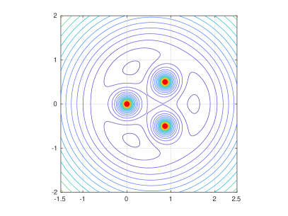
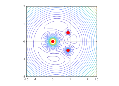
Figure 2: Level curves of the amended potential (1) with the three primaries forming an equilateral triangle. (a) Equal masses: m1=m2=m3=1/3subscript𝑚1subscript𝑚2subscript𝑚313m_{1}=m_{2}=m_{3}=1/3; (b) Different masses: m1=1/16subscript𝑚1116m_{1}=1/16, m2=3/16subscript𝑚2316m_{2}=3/16, m3=12/16subscript𝑚31216m_{3}=12/16 with the heaviest primary located at the origin.

With our approach, there are three difficulties that must be resolved in order to be successful:

  1. 1.

    The potential V𝑉V (and its gradient) is singular at the three primaries.

  2. 2.

    When the mass of a primary tends to zero, several critical points of V𝑉V tend to that primary.

  3. 3.

    As masses (not close to zero) are varied, the number of critical points of V𝑉V may change due to bifurcations taking place.

When all masses are uniformly bounded away from zero, the singularities at the primaries (case 1) can be handled by proving that no critical points can reside in certain small disks centered at the primaries. This is explained further in section 2.2.

For masses approaching zero (case 2), we end up with a multi-restricted111A restricted n𝑛n-body problem is said to be of type m+k𝑚𝑘m+k is there are m𝑚m bodies with positive mass and k𝑘k weightless bodies, and n=m+k𝑛𝑚𝑘n=m+k. problem of type 2+2222+2 (m10subscript𝑚10m_{1}\to 0) or of type 1+3131+3 (m10subscript𝑚10m_{1}\to 0 and m20subscript𝑚20m_{2}\to 0). Both scenarios can be resolved by desingularizing the potential V𝑉V along the circle zp3=1norm𝑧subscript𝑝31\|z-p_{3}\|=1. More about this in sections 4 and  6.3.1.

Out of these difficulties, the bifurcations (case 3) are the easiest to resolve. In principle, this only requires verifying the sign of certain combinations of partial derivatives of the potential V𝑉V. We will address this in section 6.5.

2.1 The mass space {\mathcal{M}}

Without loss of generality, we may assume that the masses of the primaries are normalized m1+m2+m3=1subscript𝑚1subscript𝑚2subscript𝑚31m_{1}+m_{2}+m_{3}=1 and ordered 0<m1m2m30subscript𝑚1subscript𝑚2subscript𝑚30<m_{1}\leq m_{2}\leq m_{3}. Call this set {\mathcal{M}}:

={m3:m1+m2+m3=1 and 0<m1m2m3}.conditional-set𝑚superscript3subscript𝑚1subscript𝑚2subscript𝑚31 and 0subscript𝑚1subscript𝑚2subscript𝑚3{\mathcal{M}}=\{m\in\mathbb{R}^{3}\colon m_{1}+m_{2}+m_{3}=1\textrm{ and }0<m_{1}\leq m_{2}\leq m_{3}\}. (2)

We illustrate the unordered and ordered mass space in Figure 3. Note that the midpoint of the large triangle corresponds to all masses being equal: m=(13,13,13)𝑚131313m=(\tfrac{1}{3},\tfrac{1}{3},\tfrac{1}{3}).

\psfrag{l1}{$m=(1,0,0)$}\psfrag{L2}{$m=(0,\tfrac{1}{2},\tfrac{1}{2})$}\psfrag{L3}{$m=(0,0,1)$}\psfrag{L4}{$m^{\star}$}\psfrag{L5}{$m=(\tfrac{1}{3},\tfrac{1}{3},\tfrac{1}{3})$}\includegraphics[width=173.44534pt]{./pictures/configurations4b.eps}
\psfrag{l1}{$m=(1,0,0)$}\psfrag{L2}{$m=(0,\tfrac{1}{2},\tfrac{1}{2})$}\psfrag{L3}{$m=(0,0,1)$}\psfrag{L4}{$m^{\star}$}\psfrag{L5}{$m=(\tfrac{1}{3},\tfrac{1}{3},\tfrac{1}{3})$}\includegraphics[width=54.2025pt]{./pictures/mass_space_zoom1.eps}
Figure 3: (a) The normalised mass space m1+m2+m3=1subscript𝑚1subscript𝑚2subscript𝑚31m_{1}+m_{2}+m_{3}=1 in barycentric coordinates, with the region of ordered masses (0<m1m2m30subscript𝑚1subscript𝑚2subscript𝑚30<m_{1}\leq m_{2}\leq m_{3}) highlighted in a darker shade. The blue curve illustrates the set on which bifurcations take place. (b) 1/6161/6 of the normalized mass space corresponding to the space {\mathcal{M}}. The mass msuperscript𝑚m^{\star} corresponds to a cubic-type bifurcation.

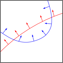
The bifurcations taking place are of two kinds: quadratic and cubic. The latter are rare, and come from the inherent 6-fold symmetry of the normalized mass space, see Figure 3. The quadratic bifucations are of a saddle-node type, in which two unique solutions approach each other, merge at the bifucration, and no longer exists beyond the point of bifurcation, see Figure 4.

Refer to caption
Refer to caption
Refer to caption
Figure 4: The typical quadratic bifurcation (blue dot), in which two solutions merge and vanish, becomes a cubic-type bifurcation at msuperscript𝑚m^{\star} due to symmetry.

In section 6.5 we will present the mathematics needed to resolve the two types of bifurcations taking place.

2.2 The configuration space 𝒞𝒞{\mathcal{C}}

Without loss of generality, we may fix the positions of the three primaries: p1=(32,+12)subscript𝑝13212p_{1}=(\tfrac{\sqrt{3}}{2},+\tfrac{1}{2}), p2=(32,12,)p_{2}=(\tfrac{\sqrt{3}}{2},-\tfrac{1}{2},), and p3=(0,0)subscript𝑝300p_{3}=(0,0), thus forming an equilateral triangle with unit length sides, as in Figure 1 b.

We begin by deriving some basic results that will be used later on. Let zV(z;m)subscript𝑧𝑉𝑧𝑚\nabla_{z}V(z;m) denote the gradient (with respect to z𝑧z) of the potential V𝑉V. A relative equilibria is then simply a solution to the equation zV(z;m)=0subscript𝑧𝑉𝑧𝑚0\nabla_{z}V(z;m)=0, i.e., a critical point of V(z;m)𝑉𝑧𝑚V(z;m).

In what follows, it will be convenient to adopt the following notation:

ri=ri(z)=zpi(i=1,2,3).formulae-sequencesubscript𝑟𝑖subscript𝑟𝑖𝑧norm𝑧subscript𝑝𝑖𝑖123r_{i}=r_{i}(z)=\|z-p_{i}\|\quad\quad(i=1,2,3). (3)

In determining the relevant configuration space, we will use the following two exlusion results (Lemma 3 and Lemma 5, respectively):

  • Assume that m31/3subscript𝑚313m_{3}\geq 1/3. If r3(z)1/3subscript𝑟3𝑧13r_{3}(z)\leq 1/3, then z𝑧z is not a critical point of the potential V𝑉V.

  • If ri(z)2subscript𝑟𝑖𝑧2r_{i}(z)\geq 2 for some i=1,2,3𝑖123i=1,2,3, then z𝑧z is not a critical point of the potential V𝑉V.

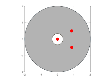
Combining these two results, we see that, for m𝑚m\in{\mathcal{M}}, all relative equilibria must satisfy 1/3r3213subscript𝑟321/3\leq r_{3}\leq 2. We will take this to be our global search region 𝒞𝒞{\mathcal{C}} in configuration space:

𝒞={z2:1/3z2}.𝒞conditional-set𝑧superscript213norm𝑧2{\mathcal{C}}=\{z\in\mathbb{R}^{2}\colon 1/3\leq\|z\|\leq 2\}. (4)

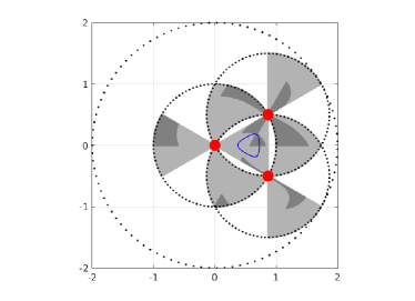
A more detailed analysis reveals that the relative eqililibria all reside in an even smaller subset of 𝒞𝒞{\mathcal{C}}, see Figure 5(a). We will, however, not use this level of detail in our computations.
Refer to caption
Refer to caption
Figure 5: The configuration space with the three primaries p1,p2,p3subscript𝑝1subscript𝑝2subscript𝑝3p_{1},p_{2},p_{3} (red points) spanning an equilateral triange. (a) The seven regions (colored light grey) in phase space where all relative equilibria must reside. When the masses are ordered, all relative equilibria are restricted to a smaller subset (colored dark grey). The blue curve illustrates the set on which bifurcations take place. (b) The global search region 𝒞={z2:1/3z2}𝒞conditional-set𝑧superscript213norm𝑧2{\mathcal{C}}=\{z\in\mathbb{R}^{2}\colon 1/3\leq\|z\|\leq 2\} of the configuration space. Note that the heaviest primary p3=(0,0)subscript𝑝300p_{3}=(0,0) does not belong to 𝒞𝒞{\mathcal{C}}.

We end this section by deriving the two exclusion results used above. The critical equation zV(z;m)=0subscript𝑧𝑉𝑧𝑚0\nabla_{z}V(z;m)=0 can be written as

(zc)+m11r1+m21r2+m31r3=0.𝑧𝑐subscript𝑚11subscript𝑟1subscript𝑚21subscript𝑟2subscript𝑚31subscript𝑟30(z-c)+m_{1}\nabla\frac{1}{r_{1}}+m_{2}\nabla\frac{1}{r_{2}}+m_{3}\nabla\frac{1}{r_{3}}=0. (5)

Note that we have

1ri=1ri2(i=1,2,3).norm1subscript𝑟𝑖1superscriptsubscript𝑟𝑖2𝑖123\left\|\nabla\frac{1}{r_{i}}\right\|=\frac{1}{r_{i}^{2}}\qquad(i=1,2,3). (6)

The following lemma provides an a priori bound on how close a solution of zV(z;m)=0subscript𝑧𝑉𝑧𝑚0\nabla_{z}V(z;m)=0 can be to one of the primaries.

Lemma 2.

Let z2𝑧superscript2z\in\mathbb{R}^{2} and set ri=ri(z)subscript𝑟𝑖subscript𝑟𝑖𝑧r_{i}=r_{i}(z). If for some i=1,2,3𝑖123i=1,2,3 we have

miri2subscript𝑚𝑖superscriptsubscript𝑟𝑖2\displaystyle\frac{m_{i}}{r_{i}^{2}} >\displaystyle> 1mi(1ri)2+ri+1,1subscript𝑚𝑖superscript1subscript𝑟𝑖2subscript𝑟𝑖1\displaystyle\frac{1-m_{i}}{(1-r_{i})^{2}}+r_{i}+1, (7)

then z𝑧z is not a critical point of the potential V𝑉V.

Proof.

First, we note that Equation (5) can be rewritten as

m11r1=m21r2m31r3(zc).subscript𝑚11subscript𝑟1subscript𝑚21subscript𝑟2subscript𝑚31subscript𝑟3𝑧𝑐m_{1}\nabla\frac{1}{r_{1}}=-m_{2}\nabla\frac{1}{r_{2}}-m_{3}\nabla\frac{1}{r_{3}}-(z-c). (8)

We use this formulation, and consider small r1subscript𝑟1r_{1}, so that the norm of the left-hand side is larger than the norms of terms appearing to the right.

Observe that (7) implies that ri<1subscript𝑟𝑖1r_{i}<1, because miri2>1subscript𝑚𝑖superscriptsubscript𝑟𝑖21\frac{m_{i}}{r_{i}^{2}}>1 and mi<1subscript𝑚𝑖1m_{i}<1. Hence, throughout the proof, we assume that r1<1subscript𝑟11r_{1}<1.

From the triangle inequality r1+r21subscript𝑟1subscript𝑟21r_{1}+r_{2}\geq 1, we have

r2subscript𝑟2\displaystyle r_{2} \displaystyle\geq 1r1,1subscript𝑟1\displaystyle 1-r_{1},
r22superscriptsubscript𝑟22\displaystyle r_{2}^{2} \displaystyle\geq (1r1)2,superscript1subscript𝑟12\displaystyle(1-r_{1})^{2},
zcnorm𝑧𝑐\displaystyle\|z-c\| \displaystyle\leq zp1+p1cr1+1.norm𝑧subscript𝑝1normsubscript𝑝1𝑐subscript𝑟11\displaystyle\|z-p_{1}\|+\|p_{1}-c\|\leq r_{1}+1.

Using this together with (7), we obtain

m21r2m31r3(zc)m2r22+m3r32+r1+1normsubscript𝑚21subscript𝑟2subscript𝑚31subscript𝑟3𝑧𝑐subscript𝑚2superscriptsubscript𝑟22subscript𝑚3superscriptsubscript𝑟32subscript𝑟11\displaystyle\left\|-m_{2}\nabla\frac{1}{r_{2}}-m_{3}\nabla\frac{1}{r_{3}}-(z-c)\right\|\leq\frac{m_{2}}{r_{2}^{2}}+\frac{m_{3}}{r_{3}^{2}}+r_{1}+1
m2(1r1)2+m3(1r1)2+r1+1=1m1(1r1)2+r1+1absentsubscript𝑚2superscript1subscript𝑟12subscript𝑚3superscript1subscript𝑟12subscript𝑟111subscript𝑚1superscript1subscript𝑟12subscript𝑟11\displaystyle\leq\frac{m_{2}}{(1-r_{1})^{2}}+\frac{m_{3}}{(1-r_{1})^{2}}+r_{1}+1=\frac{1-m_{1}}{(1-r_{1})^{2}}+r_{1}+1
<m1r12=m11r1,absentsubscript𝑚1superscriptsubscript𝑟12normsubscript𝑚11subscript𝑟1\displaystyle<\frac{m_{1}}{r_{1}^{2}}=\left\|m_{1}\nabla\frac{1}{r_{1}}\right\|,

hence (8) is not satisfied. ∎

Since we are only considering ordered masses, we always have m31/3subscript𝑚313m_{3}\geq 1/3. This fact, combined with Lemma 2, immediately gives us a uniform bound for the primary p3subscript𝑝3p_{3}.

Lemma 3.

Assume that m31/3subscript𝑚313m_{3}\geq 1/3. If r3(z)1/3subscript𝑟3𝑧13r_{3}(z)\leq 1/3, then z𝑧z is not a critical point of the potential V𝑉V.

Proof.

We verify (7) with i=3𝑖3i=3. Estimating each side of the inequality, we find

m3r321/3(1/3)2=3and1m3(1r3)2+r3+12/3(2/3)2+13+1=32+43=176<3.formulae-sequencesubscript𝑚3superscriptsubscript𝑟3213superscript1323and1subscript𝑚3superscript1subscript𝑟32subscript𝑟3123superscript23213132431763\frac{m_{3}}{r_{3}^{2}}\geq\frac{1/3}{(1/3)^{2}}=3\qquad\mathrm{and}\qquad\frac{1-m_{3}}{(1-r_{3})^{2}}+r_{3}+1\leq\frac{2/3}{(2/3)^{2}}+\frac{1}{3}+1=\frac{3}{2}+\frac{4}{3}=\frac{17}{6}<3.

Remark: For m31/3subscript𝑚313m_{3}\geq 1/3, we can exclude the slightly larger region r30.3405784subscript𝑟30.3405784r_{3}\leq 0.3405784.

Note that Lemma 2 can also be used to exclude a small disc centered at pisubscript𝑝𝑖p_{i} (i=1,2𝑖12i=1,2) whenever misubscript𝑚𝑖m_{i} is not too small. As an example, if miε>0subscript𝑚𝑖𝜀0m_{i}\geq\varepsilon>0, then we can exclude the disc ri12εsubscript𝑟𝑖12𝜀r_{i}\leq\tfrac{1}{2}\sqrt{\varepsilon}.

Another exclusion principle is given by the following result.

Lemma 4.

Let z2𝑧superscript2z\in\mathbb{R}^{2} and set ri=ri(z)subscript𝑟𝑖subscript𝑟𝑖𝑧r_{i}=r_{i}(z). If for some i=1,2,3𝑖123i=1,2,3 we have

ri1subscript𝑟𝑖1\displaystyle r_{i}-1 >\displaystyle> 1mi(1ri)2+miri2,1subscript𝑚𝑖superscript1subscript𝑟𝑖2subscript𝑚𝑖superscriptsubscript𝑟𝑖2\displaystyle\frac{1-m_{i}}{(1-r_{i})^{2}}+\frac{m_{i}}{r_{i}^{2}}, (9)

then z𝑧z is not a critical point of the potential V𝑉V.

Proof.

The proof uses the idea that we may rewrite Equation 5 as

m11r1+m21r2+m31r3=(zc).subscript𝑚11subscript𝑟1subscript𝑚21subscript𝑟2subscript𝑚31subscript𝑟3𝑧𝑐m_{1}\nabla\frac{1}{r_{1}}+m_{2}\nabla\frac{1}{r_{2}}+m_{3}\nabla\frac{1}{r_{3}}=-(z-c). (10)

Without any loss of the generality, we may assume that i=3𝑖3i=3 and shift coordinate frame so that p3subscript𝑝3p_{3} is situated at the origin. Then z=zp3=r3norm𝑧norm𝑧subscript𝑝3subscript𝑟3\|z\|=\|z-p_{3}\|=r_{3}, and from (9) (with i=3𝑖3i=3) it follows that r3>1subscript𝑟31r_{3}>1. This, together with the triangle inequality, gives

zczcr31.norm𝑧𝑐norm𝑧norm𝑐subscript𝑟31\displaystyle\|z-c\|\geq\|z\|-\|c\|\geq r_{3}-1. (11)

Here we use the fact that the center of mass c𝑐c is located within the triangle spanned by the three primaries, and therefore c1norm𝑐1\|c\|\leq 1.

Applying the triangle inequality again, we have ri+1r3subscript𝑟𝑖1subscript𝑟3r_{i}+1\geq r_{3} (i=1,2𝑖12i=1,2), from which it follows that

rir31andri2(r31)2(i=1,2).formulae-sequencesubscript𝑟𝑖subscript𝑟31andsuperscriptsubscript𝑟𝑖2superscriptsubscript𝑟312𝑖12r_{i}\geq r_{3}-1\qquad\mathrm{and}\qquad r_{i}^{2}\geq(r_{3}-1)^{2}\qquad\qquad(i=1,2). (12)

Therefore we obtain the following estimate (we use (6,12,11))

m11r1+m21r2+m31r3m1r12+m2r22+m3r32normsubscript𝑚11subscript𝑟1subscript𝑚21subscript𝑟2subscript𝑚31subscript𝑟3subscript𝑚1superscriptsubscript𝑟12subscript𝑚2superscriptsubscript𝑟22subscript𝑚3superscriptsubscript𝑟32\displaystyle\left\|m_{1}\nabla\frac{1}{r_{1}}+m_{2}\nabla\frac{1}{r_{2}}+m_{3}\nabla\frac{1}{r_{3}}\right\|\leq\frac{m_{1}}{r_{1}^{2}}+\frac{m_{2}}{r_{2}^{2}}+\frac{m_{3}}{r_{3}^{2}} \displaystyle\leq
m1(r31)2+m2(r31)2+m3r32=1m3(r31)2+m3r32subscript𝑚1superscriptsubscript𝑟312subscript𝑚2superscriptsubscript𝑟312subscript𝑚3superscriptsubscript𝑟321subscript𝑚3superscriptsubscript𝑟312subscript𝑚3superscriptsubscript𝑟32\displaystyle\frac{m_{1}}{(r_{3}-1)^{2}}+\frac{m_{2}}{(r_{3}-1)^{2}}+\frac{m_{3}}{r_{3}^{2}}=\frac{1-m_{3}}{(r_{3}-1)^{2}}+\frac{m_{3}}{r_{3}^{2}} <\displaystyle< r31zc,subscript𝑟31norm𝑧𝑐\displaystyle r_{3}-1\leq\|z-c\|,

hence (10) is not satisfied. ∎

A direct consequence of Lemma 4 is the following uniform bound.

Lemma 5.

If ri(z)2subscript𝑟𝑖𝑧2r_{i}(z)\geq 2 for some i=1,2,3𝑖123i=1,2,3, then z𝑧z is not a critical point of the potential V𝑉V.

Proof.

Using only ri(z)2subscript𝑟𝑖𝑧2r_{i}(z)\geq 2, we verify (9). Indeed, a straight forward computation gives:

1mi(ri1)2+miri21mi+mi4=13mi4<1ri1.1subscript𝑚𝑖superscriptsubscript𝑟𝑖12subscript𝑚𝑖superscriptsubscript𝑟𝑖21subscript𝑚𝑖subscript𝑚𝑖413subscript𝑚𝑖41subscript𝑟𝑖1\displaystyle\frac{1-m_{i}}{(r_{i}-1)^{2}}+\frac{m_{i}}{r_{i}^{2}}\leq 1-m_{i}+\frac{m_{i}}{4}=1-\frac{3m_{i}}{4}<1\leq r_{i}-1.

3 Reparametrizing the masses

Due to the normalisation m1+m2+m3=1subscript𝑚1subscript𝑚2subscript𝑚31m_{1}+m_{2}+m_{3}=1, the mass space can be viewed as a 2-dimensional set parametrized by m1subscript𝑚1m_{1} and m2subscript𝑚2m_{2}. Instead of working directly with the masses (m1,m2)subscript𝑚1subscript𝑚2(m_{1},m_{2}), we introduce the following non-linear, singular transformation:

s=m1m1+m2andt=m1+m2,formulae-sequence𝑠subscript𝑚1subscript𝑚1subscript𝑚2and𝑡subscript𝑚1subscript𝑚2s=\frac{m_{1}}{m_{1}+m_{2}}\qquad\mathrm{and}\qquad t=m_{1}+m_{2}, (13)

The new parameters (s,t)𝑠𝑡(s,t) can be transformed back to mass space via the inverse transformation:

m1=st,m2=(1s)t,(and m3=1t).formulae-sequencesubscript𝑚1𝑠𝑡subscript𝑚21𝑠𝑡and subscript𝑚31𝑡m_{1}=st,\qquad m_{2}=(1-s)t,\qquad(\textrm{and }m_{3}=1-t). (14)

The reason for working in the mass space using (s,t)𝑠𝑡(s,t)-coordinates is as follows: when m1subscript𝑚1m_{1} and m2subscript𝑚2m_{2} tend to zero, then some relative equilibria may move in a non-continuous way and no limit exists. This makes our kind of study virtually impossible. When seen in (s,t)𝑠𝑡(s,t)-coordinates, however, the movements are regular and amenable to our computer assisted techniques.

In the (m1,m2)subscript𝑚1subscript𝑚2(m_{1},m_{2})-space, the ordered mass space {\mathcal{M}} is a right-angled triangle, see Figure 3(b). Under the transformation (13) it is mapped to a non-linear 2-dimensional region 𝒫~~𝒫\tilde{\mathcal{P}}. Taking 𝒫𝒫{\mathcal{P}} to be the rectangular hull of 𝒫~~𝒫\tilde{\mathcal{P}}, we have our new parameter region, see Figure 6. The three vertices of {\mathcal{M}} are mapped into 𝒫𝒫{\mathcal{P}} according to the following transformations:

(m1,m2)=(1/3,1/3)subscript𝑚1subscript𝑚21313\displaystyle(m_{1},m_{2})=(1/3,1/3) maps-to\displaystyle\mapsto (s,t)=(1/2,2/3)𝑠𝑡1223\displaystyle(s,t)=(1/2,2/3)
(m1,m2)=(0,1/2)subscript𝑚1subscript𝑚2012\displaystyle(m_{1},m_{2})=(0,1/2) maps-to\displaystyle\mapsto (s,t)=(0,1/2)𝑠𝑡012\displaystyle(s,t)=(0,1/2)
(m1,m2)=(0,0)subscript𝑚1subscript𝑚200\displaystyle(m_{1},m_{2})=(0,0) maps-to\displaystyle\mapsto (s,t)=([0,1/2],0).𝑠𝑡0120\displaystyle(s,t)=([0,1/2],0).

Note how the single point (m1,m2)=(0,0)subscript𝑚1subscript𝑚200(m_{1},m_{2})=(0,0) is mapped to the line segment (s,t)=([0,1/2],0)𝑠𝑡0120(s,t)=([0,1/2],0) when taking all possible limits from within {\mathcal{M}}. This desingularization is the main reason for moving to the (s,t)𝑠𝑡(s,t)-space; it gives us a better control when masses are near the multi-restricted cases m1=0subscript𝑚10m_{1}=0 and (m1,m2)=(0,0)subscript𝑚1subscript𝑚200(m_{1},m_{2})=(0,0).

\psfrag{Ptilde}{$\tilde{\mathcal{P}}$}\psfrag{st1}{$(s,t)=(0,0)$}\psfrag{st2}{$(s,t)=(\tfrac{1}{2},0)$}\psfrag{st3}{$(s,t)=(\tfrac{1}{2},\tfrac{2}{3})$}\psfrag{st4}{$(s,t)=(0,\tfrac{1}{2})$}\psfrag{st5}{$(s^{\star},t^{\star})$}\includegraphics[width=108.405pt]{./pictures/parameter_space_zoom1.eps}
\psfrag{Ptilde}{$\tilde{\mathcal{P}}$}\psfrag{st1}{$(s,t)=(0,0)$}\psfrag{st2}{$(s,t)=(\tfrac{1}{2},0)$}\psfrag{st3}{$(s,t)=(\tfrac{1}{2},\tfrac{2}{3})$}\psfrag{st4}{$(s,t)=(0,\tfrac{1}{2})$}\psfrag{st5}{$(s^{\star},t^{\star})$}\psfrag{st1b}{}\psfrag{st2b}{${\mathcal{P}}_{1}$}\psfrag{st3b}{${\mathcal{P}}_{3}$}\psfrag{st4b}{}\psfrag{st5b}{${\mathcal{P}}_{2}$}\includegraphics[width=108.405pt]{./pictures/parameter_space_zoom1b.eps}
Figure 6: (a) The image 𝒫~~𝒫\tilde{\mathcal{P}} (shaded) of the ordered mass space {\mathcal{M}} under the transformation (13). Compare to Figure 3(b). The unshaded part of the rectangle 𝒫𝒫{\mathcal{P}} corresponds to unordered masses. (b) The partition 𝒫=𝒫1𝒫2𝒫3𝒫subscript𝒫1subscript𝒫2subscript𝒫3{\mathcal{P}}={\mathcal{P}}_{1}\cup{\mathcal{P}}_{2}\cup{\mathcal{P}}_{3} we will be using in this parametrization.

Based on this, we will define 𝒫={(s,t):0s12;0t23}𝒫conditional-set𝑠𝑡formulae-sequence0𝑠120𝑡23{\mathcal{P}}=\{(s,t)\colon 0\leq s\leq\frac{1}{2};0\leq t\leq\tfrac{2}{3}\}, and use the partition 𝒫=𝒫1𝒫2𝒫3𝒫subscript𝒫1subscript𝒫2subscript𝒫3{\mathcal{P}}={\mathcal{P}}_{1}\cup{\mathcal{P}}_{2}\cup{\mathcal{P}}_{3} as illustrated in Figure 6. More precisely we use

𝒫1=[0,0.5]×[0,0.55],𝒫2=[0,0.5]×[0.58,0.67],𝒫3=[0,0.5]×[0.55,0.58].formulae-sequencesubscript𝒫100.500.55formulae-sequencesubscript𝒫200.50.580.67subscript𝒫300.50.550.58{\mathcal{P}}_{1}=[0,0.5]\times[0,0.55],\quad{\mathcal{P}}_{2}=[0,0.5]\times[0.58,0.67],\quad{\mathcal{P}}_{3}=[0,0.5]\times[0.55,0.58].

Note that each of the three partition elements contain points from 𝒫𝒫~𝒫~𝒫{\mathcal{P}}\setminus\tilde{\mathcal{P}}. Such points correspond to unordered masses, and we will automatically remove most them from our computations. In the following, when we say that 𝒫isubscript𝒫𝑖{\mathcal{P}}_{i} has some property, we mean that the ordered parameters 𝒫i~=𝒫i𝒫~~subscript𝒫𝑖subscript𝒫𝑖~𝒫\tilde{{\mathcal{P}}_{i}}={\mathcal{P}}_{i}\cap\tilde{{\mathcal{P}}} have that property.

The three partition elements 𝒫1,𝒫2,𝒫3subscript𝒫1subscript𝒫2subscript𝒫3{\mathcal{P}}_{1},{\mathcal{P}}_{2},{\mathcal{P}}_{3} have the following properties:

  • For each (s,t)𝒫1𝑠𝑡subscript𝒫1(s,t)\in{\mathcal{P}}_{1}, there are exactly 8 solutions in 𝒞𝒞{\mathcal{C}}.

  • For each (s,t)𝒫2𝑠𝑡subscript𝒫2(s,t)\in{\mathcal{P}}_{2}, there are exactly 10 solutions in 𝒞𝒞{\mathcal{C}}.

  • For each (s,t)𝒫3𝑠𝑡subscript𝒫3(s,t)\in{\mathcal{P}}_{3}, there are between 8 and 10 solutions in 𝒞𝒞{\mathcal{C}}.

Let us describe these three regions in more detail. In subsequent sections, we will prove that these descriptions are accurate.

For (s,t)𝒫2𝑠𝑡subscript𝒫2(s,t)\in{\mathcal{P}}_{2} no bifurcations take place in 𝒞𝒞{\mathcal{C}}; exactly ten solutions exist but never come close to each other or a primary. This is the easiest region to account for. Also for (s,t)𝒫1𝑠𝑡subscript𝒫1(s,t)\in{\mathcal{P}}_{1} there are no bifurcations in 𝒞𝒞{\mathcal{C}}; exactly eight solutions exist. This region, however, includes parameters corresponding to arbitrarily small masses which presents other complications that must be resolved; more about this in section 6.3.1. The remaining set 𝒫3subscript𝒫3{\mathcal{P}}_{3} contains all parameters for which a bifucation occurs. As discussed in section 2.1, there are two bifurcation types that we must account for; quadratic and cubic. These bifurcations only take place in a small subset 𝒞2subscript𝒞2{\mathcal{C}}_{2} of the full configuration space. For (s,t)𝒫3𝑠𝑡subscript𝒫3(s,t)\in{\mathcal{P}}_{3}, there can be 1, 2 or 3 solutions in 𝒞2subscript𝒞2{\mathcal{C}}_{2}. In the remaining space 𝒞1=𝒞𝒞2subscript𝒞1𝒞subscript𝒞2{\mathcal{C}}_{1}={\mathcal{C}}\setminus{\mathcal{C}}_{2} there are exactly seven solutions, all isolated from each other and the primaries. Summing up, when (s,t)𝒫3𝑠𝑡subscript𝒫3(s,t)\in{\mathcal{P}}_{3} we have 8, 9 or 10 solutions in 𝒞𝒞{\mathcal{C}} .

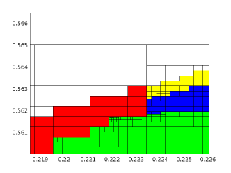
In the ideal setting, 𝒫3subscript𝒫3{\mathcal{P}}_{3} would correspond to the transformed (blue) bifurcation curve illustrated in Figure 6. It would bisect 𝒫~~𝒫\tilde{\mathcal{P}}, acting as a common boundary line separating 𝒫~1subscript~𝒫1\tilde{\mathcal{P}}_{1} from 𝒫~2subscript~𝒫2\tilde{\mathcal{P}}_{2}. Our approach, however, will build upon finite resolution computations, and therefore 𝒫2subscript𝒫2{\mathcal{P}}_{2} will be constructed as a rectangular subset of 𝒫𝒫{\mathcal{P}}, covering the entire bifurcation curve, see Figure 6.

4 Polar coordinates

Given the shape of the configuration space (4), and how the solutions behave when masses become small, it makes sense to work in polar coordinates centered at the heaviest primary p3=(0,0)subscript𝑝300p_{3}=(0,0). In these coordinates the lighter primaries become p1=(1,π/6)subscript𝑝11𝜋6p_{1}=(1,\pi/6) and p2=(1,π/6)subscript𝑝21𝜋6p_{2}=(1,-\pi/6).

For convenience, let us define

α1=π/6,α2=π/6.formulae-sequencesubscript𝛼1𝜋6subscript𝛼2𝜋6\alpha_{1}=\pi/6,\qquad\alpha_{2}=-\pi/6.

Let (z1|z2)conditionalsubscript𝑧1subscript𝑧2(z_{1}|z_{2}) denote the scalar product on 2superscript2\mathbb{R}^{2}. Given z=(rcosϕ,rsinϕ)𝑧𝑟italic-ϕ𝑟italic-ϕz=(r\cos\phi,r\sin\phi), we have

zc2superscriptnorm𝑧𝑐2\displaystyle\|z-c\|^{2} =\displaystyle= (zm1p1m2p2|zm1p1m2p2)=𝑧subscript𝑚1subscript𝑝1conditionalsubscript𝑚2subscript𝑝2𝑧subscript𝑚1subscript𝑝1subscript𝑚2subscript𝑝2absent\displaystyle(z-m_{1}p_{1}-m_{2}p_{2}|z-m_{1}p_{1}-m_{2}p_{2})=
z22m1(p1|z)2m2(p2|z)+2m1m2(p1|p2)+p12+p22,superscript𝑧22subscript𝑚1conditionalsubscript𝑝1𝑧2subscript𝑚2conditionalsubscript𝑝2𝑧2subscript𝑚1subscript𝑚2conditionalsubscript𝑝1subscript𝑝2superscriptsubscript𝑝12superscriptsubscript𝑝22\displaystyle z^{2}-2m_{1}(p_{1}|z)-2m_{2}(p_{2}|z)+2m_{1}m_{2}(p_{1}|p_{2})+p_{1}^{2}+p_{2}^{2},
(pi|z)conditionalsubscript𝑝𝑖𝑧\displaystyle(p_{i}|z) =\displaystyle= rcos(φαi),i=1,2.formulae-sequence𝑟𝜑subscript𝛼𝑖𝑖12\displaystyle r\cos(\varphi-\alpha_{i}),\quad i=1,2.

It follows that

zc2=r22m1rcos(φπ/6)2m2rcos(φ+π/6)+g(m1,m2)superscriptnorm𝑧𝑐2superscript𝑟22subscript𝑚1𝑟𝜑𝜋62subscript𝑚2𝑟𝜑𝜋6𝑔subscript𝑚1subscript𝑚2\|z-c\|^{2}=r^{2}-2m_{1}r\cos(\varphi-\pi/6)-2m_{2}r\cos(\varphi+\pi/6)+g(m_{1},m_{2})

where g(m1,m2)𝑔subscript𝑚1subscript𝑚2g(m_{1},m_{2}) depends only on the masses and not on z𝑧z. Therefore we can ignore g𝑔g when studying spatial derivatives of the potential V𝑉V.

Note that, for i=1,2𝑖12i=1,2, we have

ri2=(zpi)2=z22(pi|z)+pi2=r22rcos(φαi)+1.superscriptsubscript𝑟𝑖2superscript𝑧subscript𝑝𝑖2superscript𝑧22conditionalsubscript𝑝𝑖𝑧superscriptsubscript𝑝𝑖2superscript𝑟22𝑟𝜑subscript𝛼𝑖1\displaystyle r_{i}^{2}=(z-p_{i})^{2}=z^{2}-2(p_{i}|z)+p_{i}^{2}=r^{2}-2r\cos(\varphi-\alpha_{i})+1.

Therefore, if we define

d(r,α)=(r22rcosα+1)1/2,𝑑𝑟𝛼superscriptsuperscript𝑟22𝑟𝛼112d(r,\alpha)=\left(r^{2}-2r\cos\alpha+1\right)^{1/2}, (15)

then for i=1,2𝑖12i=1,2 we have

ri(r,φ)=d(r,φαi).subscript𝑟𝑖𝑟𝜑𝑑𝑟𝜑subscript𝛼𝑖r_{i}(r,\varphi)=d(r,\varphi-\alpha_{i}).

Concluding, in polar coordinates, we obtain the new expression for the amended potential (compare to (1)):

V(r,φ;m)=V0(r)+m1W(r,φα1)+m2W(r,φα2)+g(m1,m2)𝑉𝑟𝜑𝑚subscript𝑉0𝑟subscript𝑚1𝑊𝑟𝜑subscript𝛼1subscript𝑚2𝑊𝑟𝜑subscript𝛼2𝑔subscript𝑚1subscript𝑚2V(r,\varphi;m)=V_{0}(r)+m_{1}W(r,\varphi-\alpha_{1})+m_{2}W(r,\varphi-\alpha_{2})+g(m_{1},m_{2}) (16)

where

V0(r)=r22+m3randW(r,α)=1d(r,α)rcos(α).formulae-sequencesubscript𝑉0𝑟superscript𝑟22subscript𝑚3𝑟and𝑊𝑟𝛼1𝑑𝑟𝛼𝑟𝛼V_{0}(r)=\frac{r^{2}}{2}+\frac{m_{3}}{r}\quad\mathrm{and}\quad W(r,\alpha)=\frac{1}{d(r,\alpha)}-r\cos(\alpha).

Taking partial derivatives, the gradient of the potential (16) is given by

Vr(r,φ;m)𝑉𝑟𝑟𝜑𝑚\displaystyle\frac{\partial V}{\partial r}(r,\varphi;m) =\displaystyle= rm3r2+m1Wr(r,φα1)+m2Wr(r,φα2),𝑟subscript𝑚3superscript𝑟2subscript𝑚1𝑊𝑟𝑟𝜑subscript𝛼1subscript𝑚2𝑊𝑟𝑟𝜑subscript𝛼2\displaystyle r-\frac{m_{3}}{r^{2}}+m_{1}\frac{\partial W}{\partial r}(r,\varphi-\alpha_{1})+m_{2}\frac{\partial W}{\partial r}(r,\varphi-\alpha_{2}), (17)
Vφ(r,φ;m)𝑉𝜑𝑟𝜑𝑚\displaystyle\frac{\partial V}{\partial\varphi}(r,\varphi;m) =\displaystyle= m1Wα(r,φα1)+m2Wα(r,φα2),subscript𝑚1𝑊𝛼𝑟𝜑subscript𝛼1subscript𝑚2𝑊𝛼𝑟𝜑subscript𝛼2\displaystyle m_{1}\frac{\partial W}{\partial\alpha}(r,\varphi-\alpha_{1})+m_{2}\frac{\partial W}{\partial\alpha}(r,\varphi-\alpha_{2}), (18)

where

Wα(r,α)𝑊𝛼𝑟𝛼\displaystyle\frac{\partial W}{\partial\alpha}(r,\alpha) =\displaystyle= rsinα(11d(r,α)3),𝑟𝛼11𝑑superscript𝑟𝛼3\displaystyle r\sin\alpha\left(1-\frac{1}{d(r,\alpha)^{3}}\right),
Wr(r,α)𝑊𝑟𝑟𝛼\displaystyle\frac{\partial W}{\partial r}(r,\alpha) =\displaystyle= rcosαd(r,α)3cosα.𝑟𝛼𝑑superscript𝑟𝛼3𝛼\displaystyle-\frac{r-\cos\alpha}{d(r,\alpha)^{3}}-\cos\alpha.

Note that (18) has a factor r𝑟r in both terms. We rescale this equation by a factor 1/r1𝑟1/r and 1/(m1+m2)1subscript𝑚1subscript𝑚21/(m_{1}+m_{2}). In the (s,t)𝑠𝑡(s,t) parameters this gives us

F1(r,φ;s,t)subscript𝐹1𝑟𝜑𝑠𝑡\displaystyle F_{1}(r,\varphi;s,t) =\displaystyle= r1tr2+stWr(r,φα1)+(1s)tWr(r,φα2),𝑟1𝑡superscript𝑟2𝑠𝑡𝑊𝑟𝑟𝜑subscript𝛼11𝑠𝑡𝑊𝑟𝑟𝜑subscript𝛼2\displaystyle r-\frac{1-t}{r^{2}}+st\frac{\partial W}{\partial r}(r,\varphi-\alpha_{1})+(1-s)t\frac{\partial W}{\partial r}(r,\varphi-\alpha_{2}), (19)
F2(r,φ;s,t)subscript𝐹2𝑟𝜑𝑠𝑡\displaystyle F_{2}(r,\varphi;s,t) =\displaystyle= sWα(r,φα1)+(1s)Wα(r,φα2),𝑠superscript𝑊𝛼𝑟𝜑subscript𝛼11𝑠superscript𝑊𝛼𝑟𝜑subscript𝛼2\displaystyle s\frac{\partial W^{\star}}{\partial\alpha}(r,\varphi-\alpha_{1})+(1-s)\frac{\partial W^{\star}}{\partial\alpha}(r,\varphi-\alpha_{2}), (20)

where

Wα(r,α)=1rWα(r,α)=sinα(11d(r,α)3),superscript𝑊𝛼𝑟𝛼1𝑟𝑊𝛼𝑟𝛼𝛼11𝑑superscript𝑟𝛼3\frac{\partial W^{\star}}{\partial\alpha}(r,\alpha)=\frac{1}{r}\frac{\partial W}{\partial\alpha}(r,\alpha)=\sin\alpha\left(1-\frac{1}{d(r,\alpha)^{3}}\right),

This F(r,φ;s,t)𝐹𝑟𝜑𝑠𝑡F(r,\varphi;s,t) will be used in place of zV(z;m)subscript𝑧𝑉𝑧𝑚\nabla_{z}V(z;m) appearing in the previous sections. Zeros of F𝐹F correspond to critical points of V𝑉V, and these correspond to relative equilibria.

5 General strategy and key results

Recall that we want to determine the number of solutions to zV(z;m)=0subscript𝑧𝑉𝑧𝑚0\nabla_{z}V(z;m)=0, and to understand how these behave within 𝒞𝒞{\mathcal{C}} when the masses vary within {\mathcal{M}} (see Main Problem 1). For this to succeed, we must have a means of locating all solutions to the critical equation, and a way to analyze the various bifurcations that are possible as the masses vary.

As mentioned in section 1 our overall goal is to construct a completely analytic proof of following theorem:

Theorem 6.

For each m𝑚m\in{\mathcal{M}} there are exactly 8,9 or 10 relative equilibria (i.e., solutions to the critical equation zV(z;m)=0subscript𝑧𝑉𝑧𝑚0\nabla_{z}V(z;m)=0) in 𝒞𝒞{\mathcal{C}}.

This result was originally established by Barros and Leandro [3] using algebraic techniques. Developing analytic tools for the proof, we hope to apply these to harder instances of the n𝑛n-body problem that are not within reach using algebraic methods.

In our new setting, using the (s,t)𝑠𝑡(s,t)-coordinates together with polar coordinates (described in Sections 3 and 4), the critical equation is transformed into its equivalent form F(r,φ;s,t)=0𝐹𝑟𝜑𝑠𝑡0F(r,\varphi;s,t)=0. As explained earlier, this form is better suited for our approach, where set-valued numerical computations will play a major role.

Before going into the details of the computations used as part of our computer-assisted framework, we present the following key results. We will use three different techniques: finding the exact number of solutions for given parameters (s,t)𝑠𝑡(s,t); proving that no bifurcations take place for a range of parameters; and controlling the number of solutions when when a bifurcation takes place.

We begin by determining the number of solutions for two different parameters.

Theorem 7.

Consider the critical equation F(r,φ;s,t)=0𝐹𝑟𝜑𝑠𝑡0F(r,\varphi;s,t)=0 for the 3+1313+1 body problem.

  • (a)

    For parameters (s,t)=(1/4,1/4)𝑠𝑡1414(s,t)=(1/4,1/4), there are exactly 8 solutions in 𝒞𝒞{\mathcal{C}}.

  • (b)

    For parameters (s,t)=(9/20,3/5)𝑠𝑡92035(s,t)=(9/20,3/5), there are exactly 10 solutions in 𝒞𝒞{\mathcal{C}}.

Note that (s,t)=(1/4,1/4)𝒫1𝑠𝑡1414subscript𝒫1(s,t)=(1/4,1/4)\in{\mathcal{P}}_{1} and (s,t)=(9/20,3/5)𝒫2𝑠𝑡92035subscript𝒫2(s,t)=(9/20,3/5)\in{\mathcal{P}}_{2}, as discussed in Section 3.

Combining the results of Theorem 7 with a criterion that ensures that no bifurcations are taking place (see Section 6.3), we can extend the two solution counts to the two connected regions 𝒫1subscript𝒫1{\mathcal{P}}_{1} and 𝒫2subscript𝒫2{\mathcal{P}}_{2}, respectively:

Theorem 8.

Consider the critical equation F(r,φ;s,t)=0𝐹𝑟𝜑𝑠𝑡0F(r,\varphi;s,t)=0 for the 3+1313+1 body problem.

  • (a)

    For all parameters (s,t)𝒫1𝑠𝑡subscript𝒫1(s,t)\in{\mathcal{P}}_{1}, no solution in 𝒞𝒞{\mathcal{C}} bifurcates.

  • (b)

    For all parameters (s,t)𝒫2𝑠𝑡subscript𝒫2(s,t)\in{\mathcal{P}}_{2}, no solution in 𝒞𝒞{\mathcal{C}} bifurcates.

It follows that the number of solutions in 𝒫1subscript𝒫1{\mathcal{P}}_{1} and 𝒫2subscript𝒫2{\mathcal{P}}_{2} is constant (8 and 10, respectively).

For the remaining part 𝒫3subscript𝒫3{\mathcal{P}}_{3} of the parameter space, we must be a bit more detailed. As discussed in Section 7, we will split the configuration space into two connected components: 𝒞=𝒞1𝒞2𝒞subscript𝒞1subscript𝒞2{\mathcal{C}}={\mathcal{C}}_{1}\cup{\mathcal{C}}_{2}, thus isolating the region where all bifurcations occur.

Theorem 9.

Consider the critical equation F(r,φ;s,t)=0𝐹𝑟𝜑𝑠𝑡0F(r,\varphi;s,t)=0 for the 3+1313+1 body problem.

  • (a)

    For all parameters (s,t)𝒫3𝑠𝑡subscript𝒫3(s,t)\in{\mathcal{P}}_{3}, there are exactly 7 solutions in 𝒞1subscript𝒞1{\mathcal{C}}_{1}.

  • (b)

    For all parameters (s,t)𝒫3𝑠𝑡subscript𝒫3(s,t)\in{\mathcal{P}}_{3}, there are 1, 2, or 3 solutions in 𝒞2subscript𝒞2{\mathcal{C}}_{2}.

Theorem 6 now follows from the combination of Theorem 7, 8, and 9. In what follows, we will justify each of the three steps described above.

6 Computational techniques

Here we present the computational techniques that we need to employ in order to establish our main theorem. We also discuss the underlying set-valued methods used later on in the computer-assisted proofs.

6.1 Set-valued mathematics

We begin by giving a very brief introduction to set-valued mathematics and rigorous numerics. For more in-depth accounts we refer to e.g. [11, 14].

We will exclusively work with compact boxes x in nsuperscript𝑛{\mathbb{R}}^{n}, represented as vectors whose components are compact intervals: x=(x1,,xn)xsubscriptx1subscriptx𝑛\textbf{{x}}=(\textbf{{x}}_{1},\dots,\textbf{{x}}_{n}), where xi={x:x¯ixx¯i}subscriptx𝑖conditional-set𝑥subscript¯𝑥𝑖𝑥subscript¯𝑥𝑖\textbf{{x}}_{i}=\{x\in{\mathbb{R}}\colon\underline{x}_{i}\leq x\leq\overline{x}_{i}\} for i=1,,n𝑖1𝑛i=1,\dots,n.

Given en explicit formula for a function f:nm:𝑓superscript𝑛superscript𝑚f\colon{\mathbb{R}}^{n}\to{\mathbb{R}}^{m}, we can form its interval extension (which we also denote by f𝑓f), by extending each real operation by its interval counterpart. As long as the resulting interval image f(x)𝑓xf(\textbf{{x}}) is well-defined, we always have the following inclusion property:

range(f;x)={f(x):xx}f(x).range𝑓xconditional-set𝑓𝑥𝑥x𝑓x\mathrm{range}(f;\textbf{{x}})=\{f(x)\colon x\in\textbf{{x}}\}\subseteq f(\textbf{{x}}). (21)

The main benefit of moving from real-valued to interval-valued analysis is the ability to discretize continuous problems while retaining full control of the discretisation errors. Indeed, whilst the exact range of a function range(f;x)range𝑓x\mathrm{range}(f;\textbf{{x}}) is hard to compute, its interval image f(x)𝑓xf(\textbf{{x}}) can be found by a finite computation. In practice, the interval image is computed via a finite sequence of numerical operations. Carefully crafted libraries using directed rounding ensures that the numerical output respects the mathematical incusion propery of (21).

6.2 Equation solving and safe exclusions

We begin by stating what is known as the exclusion principle:

Theorem 10.

If f(x) is well-defined and if 0f(x)0𝑓x0\notin f(\textbf{{x}}), then f𝑓f has no zero in x.

The proof is an immediate consequence of (21). The exclusion principle can be used in an adaptive bisection scheme, gradually discarding subsets of a global search space X. At each stage of the bisection process, a (possibly empty) collection of subsets x1,,xnsubscriptx1subscriptx𝑛\textbf{{x}}_{1},\dots,\textbf{{x}}_{n} remain, whose union must contain all zeros of f𝑓f. Note, however, that this does not imply that f(x)=0𝑓𝑥0f(x)=0 has any solutions; we have only discarded subsets of X where we are certain that no zeros of f𝑓f reside. In order to prove the existence of zeros, we need an addition result.

Let fC1(X,n)𝑓superscript𝐶1Xsuperscript𝑛f\in C^{1}(\textbf{{X}},{\mathbb{R}}^{n}), where Dom(f)=XnDom𝑓Xsuperscript𝑛\mathrm{Dom}(f)=\textbf{{X}}\subseteq{\mathbb{R}}^{n}. Given an interval vector xXxX\textbf{{x}}\subset\textbf{{X}}, a point xˇxˇ𝑥x\check{x}\in\textbf{{x}}, and an invertible n×n𝑛𝑛n\times n matrix C𝐶C, we define the Krawczyk operator [6, 11] as

Kf(x;xˇ;C)=f(xˇ)Cf(xˇ)+(ICDf(x))(xxˇ).subscript𝐾𝑓xˇ𝑥𝐶𝑓ˇ𝑥𝐶𝑓ˇ𝑥𝐼𝐶𝐷𝑓xxˇ𝑥K_{f}(\textbf{{x}};\check{x};C)=f(\check{x})-C\cdot f(\check{x})+\big{(}I-C\cdot Df(\textbf{{x}})\big{)}\cdot(\textbf{{x}}-\check{x}). (22)

Popular choices are xˇ=mid(x)ˇ𝑥midx\check{x}=\mathrm{mid}(\textbf{{x}}) and C=mid([Df(xˇ)])1𝐶midsuperscriptdelimited-[]𝐷𝑓ˇ𝑥1C=\mathrm{mid}([Df(\check{x})])^{-1}, resulting in Newton-like convergence rates near simple zeros.

Theorem 11.

Assume that Kf(x;xˇ;C)subscript𝐾𝑓xˇ𝑥𝐶K_{f}(\textbf{{x}};\check{x};C) is well-defined. Then the following statements hold:

  1. 1.

    If Kf(x;xˇ;C)x=subscript𝐾𝑓xˇ𝑥𝐶xK_{f}(\textbf{{x}};\check{x};C)\cap\textbf{{x}}=\emptyset, then f𝑓f has no zeros in x.

  2. 2.

    If Kf(x;xˇ;C)intxsubscript𝐾𝑓xˇ𝑥𝐶intxK_{f}(\textbf{{x}};\check{x};C)\subset\mathrm{int}\,\textbf{{x}}, then f𝑓f has a unique zero in x.

We will use this theorem together with the interval bisection scheme, were we adaptively bisect the initial search region X into subsets x that are either discarded due to the fact that 0f(x)0𝑓x0\notin f(\textbf{{x}}), kept intact because of Kf(x;xˇ;C)intxsubscript𝐾𝑓xˇ𝑥𝐶intxK_{f}(\textbf{{x}};\check{x};C)\subset\mathrm{int}\,\textbf{{x}}, or bisected for further study. On termination, this will give us an exact count on the number of zeros of f𝑓f within X.

Theorem 11 can be extended to the setting where f𝑓f also depends on some m𝑚m-dimensional parameter: f:n×mn:𝑓superscript𝑛superscript𝑚superscript𝑛f\colon{\mathbb{R}}^{n}\times{\mathbb{R}}^{m}\to{\mathbb{R}}^{n} with (x;p)f(x;p)maps-to𝑥𝑝𝑓𝑥𝑝(x;p)\mapsto f(x;p). This is what we use to establish Theorem 7.

6.3 A set-valued criterion for local uniqueness

Continuing in the set-valued, parameter dependent setting, we will explain in detail the criteria used for detecting when (and when not) a bifurcation occurs for a general system of non-linear equations, depending on some parameters. We will also derive results aimed at extracting more detailed information about some specific bifurcations that may occur.

Let us begin by considering the general problem of solving a system of (non-linear) equations

f(x;p)=0xx,pp,formulae-sequence𝑓𝑥𝑝0formulae-sequence𝑥x𝑝pf(x;p)=0\qquad x\in\textbf{{x}},\quad p\in\textbf{{p}}, (23)

where xnxsuperscript𝑛\textbf{{x}}\subset{\mathbb{R}}^{n} and pmpsuperscript𝑚\textbf{{p}}\subset{\mathbb{R}}^{m} are high-dimensional boxes. For a sufficiently smooth f:n×mn:𝑓superscript𝑛superscript𝑚superscript𝑛f\colon{\mathbb{R}}^{n}\times{\mathbb{R}}^{m}\to{\mathbb{R}}^{n}, we want to know how many solutions (23) can have. We will focus on the bifurcations and develop a criterion which will tell us when the number of solutions of (23) changes.

For now, we will suppress the parameter dependence of f𝑓f for clarity. All results that follow are extendable to the parameter-dependent setting.

An obvious condition for the local uniqueness of solutions to (23) is given by the following theorem.

Theorem 12.

Let f:nn:𝑓superscript𝑛superscript𝑛f:{\mathbb{R}}^{n}\to{\mathbb{R}}^{n} be C1superscript𝐶1C^{1}. Assume that we are given a box xnxsuperscript𝑛\textbf{{x}}\subset{\mathbb{R}}^{n} such that 0detDf(x)0𝐷𝑓x0\notin\det Df(\textbf{{x}}). Then f𝑓f is a bijection from x onto its image.

Note that Df(x)𝐷𝑓xDf(\textbf{{x}}) is a matrix with interval entries; it contains all possible Jacobian matrices Df(x)𝐷𝑓𝑥Df(x), where xx𝑥xx\in\textbf{{x}}.

Proof.

We have for x,yx𝑥𝑦xx,y\in\textbf{{x}}, xy𝑥𝑦x\neq y

f(x)f(y)=01Df(y+t(xy))𝑑t(xy)Df(x)(xy).𝑓𝑥𝑓𝑦superscriptsubscript01𝐷𝑓𝑦𝑡𝑥𝑦differential-d𝑡𝑥𝑦𝐷𝑓x𝑥𝑦f(x)-f(y)=\int_{0}^{1}Df(y+t(x-y))dt\cdot(x-y)\in Df(\textbf{{x}})\cdot(x-y). (24)

Now, since 0detDf(x)0𝐷𝑓x0\notin\det Df(\textbf{{x}}), all (point-valued) matrices in Df(x)𝐷𝑓xDf(\textbf{{x}}) are non-singular. Therefore the right-hand side of (24) cannot contain the zero vector. Hence the left-hand side f(x)f(y)𝑓𝑥𝑓𝑦f(x)-f(y) cannot vanish. ∎

This result constitutes the core of most of our computations. Given two boxes x and p, we can easily compute y=detDf(x;p)y𝐷𝑓xp\textbf{{y}}=\det Df(\textbf{{x}};\textbf{{p}}) using interval arithmetic. If 0y0y0\notin\textbf{{y}}, we know that f(;p)𝑓𝑝f(\cdot;p) is a bijection (between x and its image) for each pp𝑝pp\in\textbf{{p}}. Therefore, the equation (23) can have at most one solution in x, and such a solution cannot undergo any bifurcation when pp𝑝pp\in\textbf{{p}}.

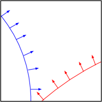
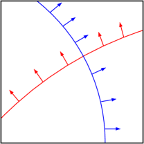
In dimension two, it is easy to illustrate the condition we are checking: the level sets of f1subscript𝑓1f_{1} and f2subscript𝑓2f_{2} must never become parallel, see Figure 7.
Refer to caption
Refer to caption
Refer to caption
Figure 7: Some of the possible configurations of level sets of f1subscript𝑓1f_{1} and f2subscript𝑓2f_{2}. The right-most configuration cannot happen under the assumptions of Theorem 12.

6.3.1 Small masses

In the case when one or two masses are very small, Theorem 12 is not practically applicable. In this situation some solutions to the critical equation are close to the primaries, and a careful analysis combined with rigorous bounds produced with computer-assistance are needed.

The strategy to study this problem is the following: we focus on each primary with small mass, and use (local) polar coordinates (ϱ,φ)italic-ϱ𝜑(\varrho,\varphi) around it to study the problem. In this setting we study the following system of equations (suppressing the dependence on masses) based on the original amended potential (1)

{Vϱ(ϱ,φ)=0,Vφ(ϱ,φ)=0.\left\{\begin{matrix}\frac{\partial V}{\partial\varrho}(\varrho,\varphi)=0,\\ \frac{\partial V}{\partial\varphi}(\varrho,\varphi)=0.\end{matrix}\right. (25)

It turns out that it is relatively easy to control the solutions of the equation Vφ(ϱ,φ)=0𝑉𝜑italic-ϱ𝜑0\frac{\partial V}{\partial\varphi}(\varrho,\varphi)=0 for φ𝜑\varphi, obtaining four curves (ϱ,φ(ϱ))italic-ϱ𝜑italic-ϱ(\varrho,\varphi(\varrho)) on which we have uniform estimates over a whole range of (m1,m2)subscript𝑚1subscript𝑚2(m_{1},m_{2}) including (0,0)00(0,0). Turning to the remaining equation

Vϱ(ϱ,φ(ϱ))=0,𝑉italic-ϱitalic-ϱ𝜑italic-ϱ0\frac{\partial V}{\partial\varrho}(\varrho,\varphi(\varrho))=0,

we study two cases separately: when m1subscript𝑚1m_{1} alone tends to zero, and when m1subscript𝑚1m_{1} and m2subscript𝑚2m_{2} both tend to zero. In both cases we can prove that any solution of (25) is of the form (ϱ,φ(ϱ))italic-ϱ𝜑italic-ϱ(\varrho,\varphi(\varrho)), and satisfies

ddϱ(Vϱ(ϱ,φ(ϱ)))0.𝑑𝑑italic-ϱ𝑉italic-ϱitalic-ϱ𝜑italic-ϱ0\frac{d}{d\varrho}\left(\frac{\partial V}{\partial\varrho}(\varrho,\varphi(\varrho))\right)\neq 0.

This implies that all solutions are regular: there are no bifurcations. We summarise our findings in a quantitative and practically applicable statement:

Theorem 13.

For 0<mi1020subscript𝑚𝑖superscript1020<m_{i}\leq 10^{-2} and R=103𝑅superscript103R=10^{-3}, any relative equilibria z𝑧z of (1) with zpiRnorm𝑧subscript𝑝𝑖𝑅\|z-p_{i}\|\leq R, i=1,2𝑖12i=1,2, is non-degenerate: it does not bifurcate.

The details of all this can be found in the appendix A, with a thorough analysis of the solutions close to the light primaries in question, and with quantitative bounds that are both useful for proving the theorem, and of general interest for further studies.

This concludes what we use to establish Theorem 8.

6.4 Lyapunov-Schmidt reduction in 2superscript2{\mathbb{R}}^{2}

If we cannot invoke Theorem 12 or 13 on a given region x×pxp\textbf{{x}}\times\textbf{{p}}, we must explore the system of equations (23) further.

Assume that the elimination of one variable (the Lyapunov-Schmidt reduction) is possible in the box x for all pp𝑝pp\in\textbf{{p}}. The condition 0fixj(x;p)0subscript𝑓𝑖subscript𝑥𝑗xp0\notin\frac{\partial f_{i}}{\partial x_{j}}(\textbf{{x}};\textbf{{p}}) for some i,j{1,,n}𝑖𝑗1𝑛i,j\in\{1,\dots,n\} is sufficient for this to be possible. It ensures that fisubscript𝑓𝑖f_{i} is strictly monotone in the variable xjsubscript𝑥𝑗x_{j} for all parameters pp𝑝pp\in\textbf{{p}}. This implies that a relation fi(x)=Csubscript𝑓𝑖𝑥𝐶f_{i}(x)=C implicitly defines xjsubscript𝑥𝑗x_{j} in terms of the other independent variables: xj=xj(x1,,xj1,xj+1,,xn)subscript𝑥𝑗subscript𝑥𝑗subscript𝑥1subscript𝑥𝑗1subscript𝑥𝑗1subscript𝑥𝑛x_{j}=x_{j}(x_{1},\dots,x_{j-1},x_{j+1},\dots,x_{n}). The domain of this parameterisation will depend on the constant C𝐶C.

From now on we will work exclusively in the two-dimensional setting, and we will once again suppress the parameter dependency for clarity. As we are interested in solutions to (23), we want to understand how the zero-level sets of f1subscript𝑓1f_{1} and f2subscript𝑓2f_{2} behave for various parameters. Without any loss of generality consider the case (i,j)=(1,1)𝑖𝑗11(i,j)=(1,1), when we have

f1x1(x)0,xx.formulae-sequencesubscript𝑓1subscript𝑥1𝑥0𝑥x\frac{\partial f_{1}}{\partial x_{1}}(x)\neq 0,\quad x\in\textbf{{x}}. (26)

Now assume also that the level set f1(x)=0subscript𝑓1𝑥0f_{1}(x)=0 forms exactly one connected component in x. Then there exists a parametrisation x1=x1(x2)subscript𝑥1subscript𝑥1subscript𝑥2x_{1}=x_{1}(x_{2}) defined on a connected domain [x2,x2+]x2superscriptsubscript𝑥2superscriptsubscript𝑥2subscriptx2[x_{2}^{-},x_{2}^{+}]\subset\textbf{{x}}_{2}, such that

f1(x1,x2)=0if and only ifx1=x1(x2).formulae-sequencesubscript𝑓1subscript𝑥1subscript𝑥20if and only ifsubscript𝑥1subscript𝑥1subscript𝑥2f_{1}(x_{1},x_{2})=0\quad\mbox{if and only if}\quad x_{1}=x_{1}(x_{2}). (27)

We can now define the reduced form of (23) as follows

g(x2)=f2(x1(x2),x2)=0,x2[x2,x2+].formulae-sequence𝑔subscript𝑥2subscript𝑓2subscript𝑥1subscript𝑥2subscript𝑥20subscript𝑥2superscriptsubscript𝑥2superscriptsubscript𝑥2g(x_{2})=f_{2}(x_{1}(x_{2}),x_{2})=0,\qquad x_{2}\in[x_{2}^{-},x_{2}^{+}]. (28)

Thus, the number of zeros of g𝑔g will determine the number of solutions to (23).

For the remaining three cases, the analogous construction would produce

g(x1)𝑔subscript𝑥1\displaystyle g(x_{1}) =\displaystyle= f2(x1,x2(x1))(i,j)=(1,2),subscript𝑓2subscript𝑥1subscript𝑥2subscript𝑥1𝑖𝑗12\displaystyle f_{2}(x_{1},x_{2}(x_{1}))\qquad(i,j)=(1,2),
g(x2)𝑔subscript𝑥2\displaystyle g(x_{2}) =\displaystyle= f1(x1(x2),x2)(i,j)=(2,1),subscript𝑓1subscript𝑥1subscript𝑥2subscript𝑥2𝑖𝑗21\displaystyle f_{1}(x_{1}(x_{2}),x_{2})\qquad(i,j)=(2,1),
g(x1)𝑔subscript𝑥1\displaystyle g(x_{1}) =\displaystyle= f1(x1,x2(x1))(i,j)=(2,2).subscript𝑓1subscript𝑥1subscript𝑥2subscript𝑥1𝑖𝑗22\displaystyle f_{1}(x_{1},x_{2}(x_{1}))\qquad(i,j)=(2,2).

To simplify notation, we will use y𝑦y as the independent variable of g𝑔g, and its domain will be denoted y=[y,y+]ysuperscript𝑦superscript𝑦\textbf{{y}}=[y^{-},y^{+}]. Note that a sufficient condition for the uniqueness of a solution of g(y)=0𝑔𝑦0g(y)=0, and hence also of (23) is

g(y)0,yy.formulae-sequencesuperscript𝑔𝑦0𝑦yg^{\prime}(y)\neq 0,\quad y\in\textbf{{y}}. (29)

It turns out that (29) can be formulated in an invariant way. We will return to the case (i,j)=(1,1)𝑖𝑗11(i,j)=(1,1) for the sake of clarity.

Implicit differentiation of (27) gives

x1(x2)=(f1x1(x1(x2),x2))1f1x2(x1(x2),x2).superscriptsubscript𝑥1subscript𝑥2superscriptsubscript𝑓1subscript𝑥1subscript𝑥1subscript𝑥2subscript𝑥21subscript𝑓1subscript𝑥2subscript𝑥1subscript𝑥2subscript𝑥2x_{1}^{\prime}(x_{2})=-\left(\frac{\partial f_{1}}{\partial x_{1}}(x_{1}(x_{2}),x_{2})\right)^{-1}\frac{\partial f_{1}}{\partial x_{2}}(x_{1}(x_{2}),x_{2}).

Applying the chain rule to (28) gives

g(x2)=f2x1(x1(x2),x2)x1(x2)+f2x2(x1(x2),x2)superscript𝑔subscript𝑥2subscript𝑓2subscript𝑥1subscript𝑥1subscript𝑥2subscript𝑥2superscriptsubscript𝑥1subscript𝑥2subscript𝑓2subscript𝑥2subscript𝑥1subscript𝑥2subscript𝑥2g^{\prime}(x_{2})=\frac{\partial f_{2}}{\partial x_{1}}(x_{1}(x_{2}),x_{2})x_{1}^{\prime}(x_{2})+\frac{\partial f_{2}}{\partial x_{2}}(x_{1}(x_{2}),x_{2})

and substituting the expression for x1(x2)superscriptsubscript𝑥1subscript𝑥2x_{1}^{\prime}(x_{2}) into this produces

g(x2)superscript𝑔subscript𝑥2\displaystyle g^{\prime}(x_{2}) =\displaystyle= (f1x1)1f1x2f2x1+f2x2superscriptsubscript𝑓1subscript𝑥11subscript𝑓1subscript𝑥2subscript𝑓2subscript𝑥1subscript𝑓2subscript𝑥2\displaystyle-\left(\frac{\partial f_{1}}{\partial x_{1}}\right)^{-1}\frac{\partial f_{1}}{\partial x_{2}}\frac{\partial f_{2}}{\partial x_{1}}+\frac{\partial f_{2}}{\partial x_{2}}
=\displaystyle= (f1x1)1(f1x1f2x2f1x2f2x1)=(f1x1)1det(Df).superscriptsubscript𝑓1subscript𝑥11subscript𝑓1subscript𝑥1subscript𝑓2subscript𝑥2subscript𝑓1subscript𝑥2subscript𝑓2subscript𝑥1superscriptsubscript𝑓1subscript𝑥11𝐷𝑓\displaystyle\left(\frac{\partial f_{1}}{\partial x_{1}}\right)^{-1}\left(\frac{\partial f_{1}}{\partial x_{1}}\frac{\partial f_{2}}{\partial x_{2}}-\frac{\partial f_{1}}{\partial x_{2}}\frac{\partial f_{2}}{\partial x_{1}}\right)=\left(\frac{\partial f_{1}}{\partial x_{1}}\right)^{-1}\det(Df).

The importance of the non-vanishing condition (26) is now clear, as is the non-vanishing determinant condition of Theorem 12.

In what follows, we will refer to the constructed function g𝑔g as the bifurcation function.

6.5 Bifurcation analysis

Having seen how to apply the Lyapunov-Schmidt reduction, we now re-introduce the parameters to f𝑓f (and thus g𝑔g). Given a bifurcation function g:y×p:𝑔ypg:\textbf{{y}}\times\textbf{{p}}\to\mathbb{R}, we would like to study the maximal number of solutions g(y;p)=0𝑔𝑦𝑝0g(y;p)=0 can have in y for pp𝑝pp\in\textbf{{p}}.

Instead of fully resolving the details of all possible bifurcations, we will use the following simple observation:

Lemma 14.

Let g𝑔g be the bifurcation function as defined in Section 6.4. Assume that for some k+𝑘superscriptk\in\mathbb{Z}^{+} we have

kgyk(y;p)0,(y,p)y×p.formulae-sequencesuperscript𝑘𝑔superscript𝑦𝑘𝑦𝑝0for-all𝑦𝑝yp\frac{\partial^{k}g}{\partial y^{k}}(y;p)\neq 0,\quad\forall(y,p)\in\textbf{{y}}\times\textbf{{p}}. (30)

Then for each pp𝑝pp\in\textbf{{p}}, the equation g(y;p)=0𝑔𝑦𝑝0g(y;p)=0 has at most k𝑘k solutions in y.

The rightmost part of Figure 7 illustrates the case k=2𝑘2k=2: the bifurcation function g𝑔g then has a quadratic behaviour.

Given a search region x×pxp\textbf{{x}}\times\textbf{{p}} for the original problem (23), we can try to find a positive integer k𝑘k such that 0g(k)(xi;p)0superscript𝑔𝑘subscriptx𝑖p0\notin g^{(k)}(\textbf{{x}}_{i};\textbf{{p}}). Here i𝑖i can be any index for which the Lyapunov-Schmidt reduction works (note that then we have yxiysubscriptx𝑖\textbf{{y}}\subset\textbf{{x}}_{i}). If we succeed, we have an upper bound on the number of solutions to g(y;p)=0𝑔𝑦𝑝0g(y;p)=0 in the region xi×py×pypsubscriptx𝑖p\textbf{{x}}_{i}\times\textbf{{p}}\supset\textbf{{y}}\times\textbf{{p}}. Note that this number translates to the original system of equations (23). By construction, the solutions to g(y;p)=0𝑔𝑦𝑝0g(y;p)=0 are in one-to-one correspondence to those of f(x;p)=0𝑓𝑥𝑝0f(x;p)=0.

For the planar circular restricted 4-body problem it turns out that we only have to consider the cases k=1,2,3𝑘123k=1,2,3. The bifurcation function g𝑔g never behaves worse than a cubic function. The actual evaluation of the increasingly complicated expressions g(k)superscript𝑔𝑘g^{(k)} is achieved by automatic differentiation. Furthermore, the Lyapunov-Schmidt reduction always succeeds in the case (i,j)=(2,2)𝑖𝑗22(i,j)=(2,2), so we always have g=g(x1)=f1(x1,x2(x1))𝑔𝑔subscript𝑥1subscript𝑓1subscript𝑥1subscript𝑥2subscript𝑥1g=g(x_{1})=f_{1}(x_{1},x_{2}(x_{1})).

We end this section by describing how we ensure that the level set f2(x)=0subscript𝑓2𝑥0f_{2}(x)=0 forms exactly one connected component in x. This is an important part of the Lyapunov-Schmidt reduction, and allows us to obtain an upper bound on the number of solutions via Lemma 14. First we verify that (i,j)=(2,2)𝑖𝑗22(i,j)=(2,2) are suitable indices by checking that 0f2x2(x)0subscript𝑓2subscript𝑥2x0\notin\frac{\partial f_{2}}{\partial x_{2}}(\textbf{{x}}). Note that this condition prevents a component of f2(x)=0subscript𝑓2𝑥0f_{2}(x)=0 forming a closed loop inside x; each component must enter and exit x. Writing x=[x1,x1+]×[x2,x2+]xsuperscriptsubscript𝑥1superscriptsubscript𝑥1superscriptsubscript𝑥2superscriptsubscript𝑥2\textbf{{x}}=[x_{1}^{-},x_{1}^{+}]\times[x_{2}^{-},x_{2}^{+}], we next verify that f2(x1,x2)<0<f2(x1+,x2+)subscript𝑓2superscriptsubscript𝑥1superscriptsubscript𝑥20subscript𝑓2superscriptsubscript𝑥1superscriptsubscript𝑥2f_{2}(x_{1}^{-},x_{2}^{-})<0<f_{2}(x_{1}^{+},x_{2}^{+}). This implies that f2subscript𝑓2f_{2} must vanish at least twice on the boundary of x. For each of the four sides sisubscripts𝑖\textbf{{s}}_{i} (i=1,,4)𝑖14(i=1,\dots,4) of the rectangle x, we compute an enclosure of the zero set zi={xsi:f2(x)=0}subscriptz𝑖conditional-set𝑥subscripts𝑖subscript𝑓2𝑥0\textbf{{z}}_{i}=\{x\in\textbf{{s}}_{i}\colon f_{2}(x)=0\}. On each such non-empty zisubscriptz𝑖\textbf{{z}}_{i}, we check that f2subscript𝑓2f_{2} is strictly increasing in its non-constant variable. This implies that i=14zisuperscriptsubscript𝑖14subscriptz𝑖\cup_{i=1}^{4}\textbf{{z}}_{i} must form two connected components w1subscript𝑤1w_{1} and w2subscript𝑤2w_{2}. Each wisubscript𝑤𝑖w_{i} is made up of either one (non-empty) zero set zjsubscriptz𝑗\textbf{{z}}_{j} or two such sets joined at a corner of x. The level set f2(x)=0subscript𝑓2𝑥0f_{2}(x)=0 crosses each of w1subscript𝑤1w_{1} and w2subscript𝑤2w_{2} transversally, and exactly once. Thus we have proved that f2(x)=0subscript𝑓2𝑥0f_{2}(x)=0 forms exactly one connected component in x.

7 Computational results

We will now describe the program used for proving the results of Section 5. Throughout all computations, we use the parameters (s,t)𝒫=[0,12]×[0,23]𝑠𝑡𝒫012023(s,t)\in{\mathcal{P}}=[0,\tfrac{1}{2}]\times[0,\tfrac{2}{3}] in place of the masses (m1,m2,m3)subscript𝑚1subscript𝑚2subscript𝑚3(m_{1},m_{2},m_{3})\in{\mathcal{M}}, as described in Section 3. We also represent the phase space variable z𝒞𝑧𝒞z\in{\mathcal{C}} in polar coordinates (r,θ)[13,2]×[π,π]𝑟𝜃132𝜋𝜋(r,\theta)\in[\tfrac{1}{3},2]\times[-\pi,\pi], and desingularize the equations as described in Section 4. This transforms the original critical equation zV(z;m)=0subscript𝑧𝑉𝑧𝑚0\nabla_{z}V(z;m)=0 into the equivalent problem F(r,φ;s,t)=0𝐹𝑟𝜑𝑠𝑡0F(r,\varphi;s,t)=0, which is more suitable for computations.

The syntax of the program is rather straight-forward:

           ./pcr4bp tol minS maxS minT maxT strategy
  • tol is the stopping tolerance used in the adaptive bisection process (used to discard subsets of the search region proved to have no zeros);

  • We consider parameters ss𝑠ss\in\textbf{{s}} satisfying minS sabsent𝑠absent\leq s\leq maxS.

  • We consider parameters tt𝑡tt\in\textbf{{t}} satisfying minT tabsent𝑡absent\leq t\leq maxT.

  • strategy determines which method we use:

    1. 1.

      Explicitly count all solutions in 𝒞𝒞{\mathcal{C}} – used for s×t𝒫st𝒫\textbf{{s}}\times\textbf{{t}}\subset{\mathcal{P}} of very small width only.

    2. 2.

      Verify that there are no bifurcations taking place in 𝒞𝒞{\mathcal{C}} for (s,t)s×t𝒫𝑠𝑡st𝒫(s,t)\in\textbf{{s}}\times\textbf{{t}}\subset{\mathcal{P}}.

    3. 3.

      Resolve all bifurcations taking place in 𝒞𝒞{\mathcal{C}} for (s,t)s×t𝒫𝑠𝑡st𝒫(s,t)\in\textbf{{s}}\times\textbf{{t}}\subset{\mathcal{P}}.

The three strategies are based on Theorem 11, Theorem 12 together with Theorem 13, and Lemma 14, respectively.

7.1 Proof of Theorem 7

We demonstrate the program by proving Theorem 7, running it on two different point-valued parameters (using strategy 1). The first one is for (s,t)=(1/4,1/4)𝑠𝑡1414(s,t)=(1/4,1/4). This corresponds to the masses m=(1/16,3/16,12/16)𝑚1163161216m=(1/16,3/16,12/16), and produces 8 solutions.

./pcr4bp 1e-6 0.25 0.25 0.25 0.25 1

============================================================
========================== pcr4bp ==========================
Started computations: Fri Mar 18 17:57:37 2022

Stopping tolerance in the search: TOL = +1.000000e-06
Parameter range for s = [+2.500000e-01, +2.500000e-01]
Parameter range for t = [+2.500000e-01, +2.500000e-01]
  This corresponds to
  m1 = [+6.250000e-02, +6.250000e-02]
  m2 = [+1.875000e-01, +1.875000e-01]
  m3 = [+7.500000e-01, +7.500000e-01]
=========================================================
Using strategy #1: Trying to get an exact count valid for
the entire parameter region.
=========================================================
Searching the full configuration space:
  C = {[+3.333333e-01, +2.000000e+00],[-3.141593e+00, +3.141593e+00]}
After bisection/Krawczyk stage:
  |smallList|  : +0
  |noList|     : +185
  |yesList|    : +8
  |tightList|  : +8
  |ndtList|    : +4
=========================================================
SUCCESS: the explicit search was conclusive.
We found exactly +8 solutions.
=========================================================
Ended computations: Fri Mar 18 17:57:37 2022
=========================================================

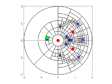
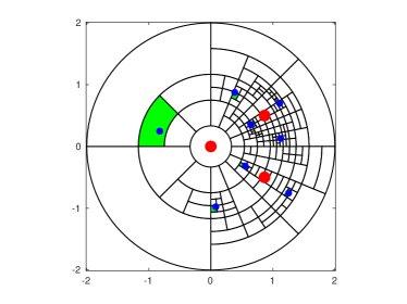
Here 𝚜𝚖𝚊𝚕𝚕𝙻𝚒𝚜𝚝𝚜𝚖𝚊𝚕𝚕𝙻𝚒𝚜𝚝{\bf\tt smallList} is empty, signaling that the bisection stage was successful and had no unresolved subdomains. 𝚗𝚘𝙻𝚒𝚜𝚝𝚗𝚘𝙻𝚒𝚜𝚝{\bf\tt noList} contains all boxes that were excluded using Theorem 10: there were 185 such boxes in this run. The eight elements of 𝚢𝚎𝚜𝙻𝚒𝚜𝚝𝚢𝚎𝚜𝙻𝚒𝚜𝚝{\bf\tt yesList} are certified to contain unique zeros of f𝑓f, according to Theorem 11. The same eight zeros are enclosed in the much smaller boxes stored in 𝚝𝚒𝚐𝚑𝚝𝙻𝚒𝚜𝚝𝚝𝚒𝚐𝚑𝚝𝙻𝚒𝚜𝚝{\bf\tt tightList}. Finally, the four boxes of 𝚗𝚍𝚝𝙻𝚒𝚜𝚝𝚗𝚍𝚝𝙻𝚒𝚜𝚝\bf\tt ndtList are close to the lighter primaries, and are proven not to contain any zeros of f𝑓f according to the exclusion results of Section 2.2. The output of this run is illustrated in Figure 8(a).
Refer to caption
Refer to caption
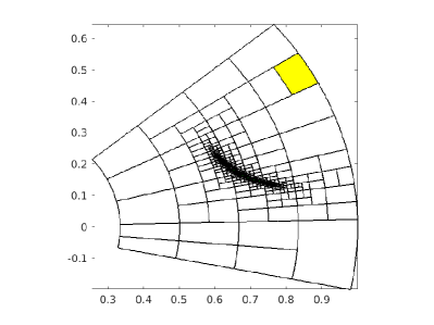
Figure 8: Relative equilibria (blue small disks) for the restricted 444–body problem. The three primaries are red large disks. Green sectors contain unique solutions. White sectors are solution-free. (a) When masses differ substantially, there are eight relative equilibria. (b) Near equal masses yield ten relative equilibria.

The second run is for (s,t)=(9/20,3/5)𝑠𝑡92035(s,t)=(9/20,3/5). This corresponds to m=(27/100,33/100,40/100)𝑚271003310040100m=(27/100,33/100,40/100), and produces 10 solutions. The output of this run is listed below, and is illustrated in Figure 8(b).

./pcr4bp 1e-6 0.45 0.45 0.60 0.60 1

============================================================
========================== pcr4bp ==========================
Started computations: Fri Mar 18 18:42:02 2022

Stopping tolerance in the search: TOL = +1.000000e-06
Parameter range for s = [+4.500000e-01, +4.500000e-01]
Parameter range for t = [+6.000000e-01, +6.000000e-01]
  This corresponds to
  m1 = [+2.700000e-01, +2.700000e-01]
  m2 = [+3.300000e-01, +3.300000e-01]
  m3 = [+4.000000e-01, +4.000000e-01]
=========================================================
Using strategy #1: Trying to get an exact count valid for
the entire parameter region.
=========================================================
Searching the full configuration space:
  C = {[+3.333333e-01, +2.000000e+00],[-3.141593e+00, +3.141593e+00]}
After bisection/Krawczyk stage:
  |smallList|  : +0
  |noList|     : +307
  |yesList|    : +10
  |tightList|  : +10
  |ndtList|    : +3
=========================================================
SUCCESS: the explicit search was conclusive.
We found exactly +10 solutions.
=========================================================
Ended computations: Fri Mar 18 18:42:02 2022
=========================================================

These two runs complete the proof of Theorem 7.

7.2 Proof of Theorem 8

Extending these results to larger domains in the (s,t)𝑠𝑡(s,t)-parameter space, we turn to Theorem 8. In order to improve execution times, we pre-split the parameter domain into smaller subsets as illustrated in Figure 9. This particular splitting is rather ad-hoc, and is based on some heuristic trial runs; other splittings would work fine too.

\psfrag{st2b}{${\mathcal{P}}_{1}$}\psfrag{st3b}{${\mathcal{P}}_{3}$}\psfrag{st5b}{${\mathcal{P}}_{2}$}\includegraphics[width=125.74689pt]{./pictures/parameter_space_zoom1b.eps}
\psfrag{st2b}{${\mathcal{P}}_{1}$}\psfrag{st3b}{${\mathcal{P}}_{3}$}\psfrag{st5b}{${\mathcal{P}}_{2}$}\includegraphics[width=106.23477pt]{./pictures/parameter_space_splitting.eps}
Figure 9: (a) The original partition 𝒫=𝒫1𝒫2𝒫3𝒫subscript𝒫1subscript𝒫2subscript𝒫3{\mathcal{P}}={\mathcal{P}}_{1}\cup{\mathcal{P}}_{2}\cup{\mathcal{P}}_{3} used in the (s,t)𝑠𝑡(s,t)-space. (b) The finer partition of 𝒫𝒫{\mathcal{P}} used in our computations (not to scale). 𝒫3subscript𝒫3{\mathcal{P}}_{3} is pre-split into three subsets, and 𝒫1subscript𝒫1{\mathcal{P}}_{1} is pre-split into four. 𝒫2subscript𝒫2{\mathcal{P}}_{2} remains intact.

We begin with the parameter set 𝒫1=[0,0.5]×[0,0.55]subscript𝒫100.500.55{\mathcal{P}}_{1}=[0,0.5]\times[0,0.55] which is pre-split into four rectangles:

𝒫1=[0,106]×[0,106][106,0.5]×[0,106][0,106]×[106,0.55][106,0.5]×[106,0.55],subscript𝒫10superscript1060superscript106superscript1060.50superscript1060superscript106superscript1060.55superscript1060.5superscript1060.55{\mathcal{P}}_{1}=[0,10^{-6}]\times[0,10^{-6}]\cup[10^{-6},0.5]\times[0,10^{-6}]\cup[0,10^{-6}]\times[10^{-6},0.55]\cup[10^{-6},0.5]\times[10^{-6},0.55],

see Figure 9(b). Note that 𝒫1~=𝒫1𝒫~~subscript𝒫1subscript𝒫1~𝒫\tilde{{\mathcal{P}}_{1}}={\mathcal{P}}_{1}\cap\tilde{\mathcal{P}} corresponds to the mass region above the bifurcation line in Figure 3(b): this region contains all small masses m1subscript𝑚1m_{1} and m2subscript𝑚2m_{2}. Examining each of the four rectangles separately, we now use strategy number 2, which means that we are attempting to verify that no bifurcations take place for these parameter ranges. We begin with (s,t)[0,106]×[0,106]𝑠𝑡0superscript1060superscript106(s,t)\in[0,10^{-6}]\times[0,10^{-6}]:

$ ./pcr4bp 1e-6 0.00 1e-6 0.00 1e-6 2

============================================================
========================== pcr4bp ==========================
Started computations: Tue Mar 22 09:32:37 2022

Stopping tolerance in the search: TOL = +1.000000e-06
Parameter range for s = [+0.000000e+00, +1.000000e-06]
Parameter range for t = [+0.000000e+00, +1.000000e-06]
  This corresponds to
  m1 = [+0.000000e+00, +1.000000e-12]
  m2 = [+0.000000e+00, +1.000000e-06]
  m3 = [+9.999990e-01, +1.000000e+00]
=========================================================
Using strategy #2: Trying to prove that no bifurcations
take place for the entire parameter region.
=========================================================
Searching the full configuration space:
  C = {[+3.333333e-01, +2.000000e+00],[-3.141593e+00, +3.141593e+00]}
After bisection/determinant stage:
  unordered masses: +0
  |smallList|     : +0
  |noList|        : +1972
  |ndgList|       : +1637
  |ndtList|       : +99
=========================================================
SUCCESS: the implicit search was conclusive.
There are no bifurcations occurring for these parameters.
=========================================================
Ended computations: Tue Mar 22 09:32:37 2022
=========================================================

We repeat the computation on the second rectangle (s,t)[106,0.5]×[0,106]𝑠𝑡superscript1060.50superscript106(s,t)\in[10^{-6},0.5]\times[0,10^{-6}]:

$ ./pcr4bp 1e-6 1e-6 0.50 0.00 1e-6 2

============================================================
========================== pcr4bp ==========================
Started computations: Tue Mar 22 09:32:47 2022

Stopping tolerance in the search: TOL = +1.000000e-06
Parameter range for s = [+1.000000e-06, +5.000000e-01]
Parameter range for t = [+0.000000e+00, +1.000000e-06]
  This corresponds to
  m1 = [+0.000000e+00, +5.000000e-07]
  m2 = [+0.000000e+00, +9.999990e-07]
  m3 = [+9.999990e-01, +1.000000e+00]
=========================================================
Using strategy #2: Trying to prove that no bifurcations
take place for the entire parameter region.
=========================================================
Searching the full configuration space:
  C = {[+3.333333e-01, +2.000000e+00],[-3.141593e+00, +3.141593e+00]}
After bisection/determinant stage:
  unordered masses: +0
  |smallList|     : +0
  |noList|        : +1453289
  |ndgList|       : +1268457
  |ndtList|       : +99963
=========================================================
SUCCESS: the implicit search was conclusive.
There are no bifurcations occurring for these parameters.
=========================================================
Ended computations: Tue Mar 22 09:34:13 2022
=========================================================

We repeat the computation on the third rectangle (s,t)[0,106]×[106,0.55]𝑠𝑡0superscript106superscript1060.55(s,t)\in[0,10^{-6}]\times[10^{-6},0.55]:

$ ./pcr4bp 1e-6 0.00 1e-6 1e-6 0.55 2

============================================================
========================== pcr4bp ==========================
Started computations: Tue Mar 22 09:34:42 2022

Stopping tolerance in the search: TOL = +1.000000e-06
Parameter range for s = [+0.000000e+00, +1.000000e-06]
Parameter range for t = [+1.000000e-06, +5.500000e-01]
  This corresponds to
  m1 = [+0.000000e+00, +5.500000e-07]
  m2 = [+9.999990e-07, +5.500000e-01]
  m3 = [+4.500000e-01, +9.999990e-01]
=========================================================
Using strategy #2: Trying to prove that no bifurcations
take place for the entire parameter region.
=========================================================
Searching the full configuration space:
  C = {[+3.333333e-01, +2.000000e+00],[-3.141593e+00, +3.141593e+00]}
After bisection/determinant stage:
  unordered masses: +954
  |smallList|     : +0
  |noList|        : +13330641
  |ndgList|       : +4592794
  |ndtList|       : +336900
NOTE: we encountered regions in parameter space that
correspond to unordered masses. These were not analyzed.
=========================================================
SUCCESS: the implicit search was conclusive.
There are no bifurcations occurring for these parameters.
=========================================================
Ended computations: Tue Mar 22 09:42:22 2022
=========================================================

Finally, we repeat the computation on the fourth rectangle (s,t)[106,0.5]×[106,0.55]𝑠𝑡superscript1060.5superscript1060.55(s,t)\in[10^{-6},0.5]\times[10^{-6},0.55]:

$ ./pcr4bp 1e-6 1e-6 0.50 1e-6 0.55 2

============================================================
========================== pcr4bp ==========================
Started computations: Tue Mar 22 09:30:32 2022

Stopping tolerance in the search: TOL = +1.000000e-06
Parameter range for s = [+1.000000e-06, +5.000000e-01]
Parameter range for t = [+1.000000e-06, +5.500000e-01]
  This corresponds to
  m1 = [+1.000000e-12, +2.750000e-01]
  m2 = [+5.000000e-07, +5.499995e-01]
  m3 = [+4.500000e-01, +9.999990e-01]
=========================================================
Using strategy #2: Trying to prove that no bifurcations
take place for the entire parameter region.
=========================================================
Searching the full configuration space:
  C = {[+3.333333e-01, +2.000000e+00],[-3.141593e+00, +3.141593e+00]}
After bisection/determinant stage:
  unordered masses: +9125
  |smallList|     : +0
  |noList|        : +2294008
  |ndgList|       : +1018710
  |ndtList|       : +160852
NOTE: we encountered regions in parameter space that
correspond to unordered masses. These were not analyzed.
=========================================================
SUCCESS: the implicit search was conclusive.
There are no bifurcations occurring for these parameters.
=========================================================
Ended computations: Tue Mar 22 09:32:10 2022
=========================================================

These four runs prove that 𝒫1subscript𝒫1{\mathcal{P}}_{1} is bifurcation free, which establishes part (a) of Theorem 8. Here we also get a report of several encountered parameter regions that are unordered; they are a consequence of the reparametrization of the mass space, and belong to the set 𝒫𝒫~𝒫~𝒫{\mathcal{P}}\setminus\tilde{\mathcal{P}}, see Figure 6. Such parameters are automatically discarded. Furthermore, ndgList contains all boxes where we have established that no bifurcations are taking place. As we are encountering parameters corresponding to both m1subscript𝑚1m_{1} and m2subscript𝑚2m_{2} becoming (arbitrarily) small, there is a significant partitioning near the lighter primaries, resulting in many boxes in ndtList.

Turning to part (b) of Theorem 8, we continue with the parameter set 𝒫2=[0,0.5]×[0.58,0.67]subscript𝒫200.50.580.67{\mathcal{P}}_{2}=[0,0.5]\times[0.58,0.67]. Note that 𝒫2𝒫~subscript𝒫2~𝒫{\mathcal{P}}_{2}\cap\tilde{\mathcal{P}} corresponds to the mass region below the bifurcation line in Figure 3(b). This region contains the point of equal masses. Again we use strategy number 2.

$ ./pcr4bp 1e-6 0.00 0.50 0.58 0.67 2

============================================================
========================== pcr4bp ==========================
Started computations: Tue Mar 22 09:30:08 2022

Stopping tolerance in the search: TOL = +1.000000e-06
Parameter range for s = [+0.000000e+00, +5.000000e-01]
Parameter range for t = [+5.800000e-01, +6.700000e-01]
  This corresponds to
  m1 = [+0.000000e+00, +3.350000e-01]
  m2 = [+2.900000e-01, +6.700000e-01]
  m3 = [+3.300000e-01, +4.200000e-01]
=========================================================
Using strategy #2: Trying to prove that no bifurcations
take place for the entire parameter region.
=========================================================
Searching the full configuration space:
  C = {[+3.333333e-01, +2.000000e+00],[-3.141593e+00, +3.141593e+00]}
After bisection/determinant stage:
  unordered masses: +3324
  |smallList|     : +0
  |noList|        : +50435
  |ndgList|       : +13145
  |ndtList|       : +13
NOTE: we encountered regions in parameter space that
correspond to unordered masses. These were not analyzed.
=========================================================
SUCCESS: the implicit search was conclusive.
There are no bifurcations occurring for these parameters.
=========================================================
Ended computations: Tue Mar 22 09:30:10 2022
=========================================================

This run proves that 𝒫2subscript𝒫2{\mathcal{P}}_{2} is bifurcation free, as claimed. Note that the computational effort was smaller than that for 𝒫1subscript𝒫1{\mathcal{P}}_{1}. This is due to the fact that we are not considering any parameters corresponding to small masses in this run. We have now completed the proof of Theorem 8.

7.3 Proof of Theorem 9

Turning to Theorem 9, we focus on the only remaining parameter set 𝒫3=[0,0.5]×[0.55,0.58]subscript𝒫300.50.550.58{\mathcal{P}}_{3}=[0,0.5]\times[0.55,0.58], which has been constructed to contain the entire line of bifurcation, see Figure 6(b). We now use strategy number 3, which means that we will locate and resolve all occurring bifurcations.

It turns out that all bifurcations take place within a small subset 𝒞2subscript𝒞2{\mathcal{C}}_{2} of the configuration space. In the complement 𝒞1=𝒞𝒞2subscript𝒞1𝒞subscript𝒞2{\mathcal{C}}_{1}={\mathcal{C}}\setminus{\mathcal{C}}_{2}, the solutions are non-degenerate and persist for all parameter values in 𝒫3subscript𝒫3{\mathcal{P}}_{3}. In light of this, the program splits the configuration space into two parts: 𝒞=𝒞1𝒞2𝒞subscript𝒞1subscript𝒞2{\mathcal{C}}={\mathcal{C}}_{1}\cup{\mathcal{C}}_{2} which are examined separately. For purely technical reasons 𝒞1subscript𝒞1{\mathcal{C}}_{1} is further divided into three subregions (named C11, C12, C13 in the output).

As explained above, 𝒫3subscript𝒫3{\mathcal{P}}_{3} is pre-split into three rectangles:

𝒫3=[0,0.2]×[0.55,0.58][0.2,0.25]×[0.55,0.58][0.25,0.5]×[0.55,0.58],subscript𝒫300.20.550.580.20.250.550.580.250.50.550.58{\mathcal{P}}_{3}=[0,0.2]\times[0.55,0.58]\cup[0.2,0.25]\times[0.55,0.58]\cup[0.25,0.5]\times[0.55,0.58],

see Figure 9(b).

We begin with (s,t)[0,0.2]×[0.55,0.58]𝑠𝑡00.20.550.58(s,t)\in[0,0.2]\times[0.55,0.58]:

$ ./pcr4bp 1e-6 0.00 0.20 0.55 0.58 3

============================================================
========================== pcr4bp ==========================
Started computations: Tue Mar 22 09:45:19 2022

Stopping tolerance in the search: TOL = +1.000000e-06
Parameter range for s = [+0.000000e+00, +2.000000e-01]
Parameter range for t = [+5.500000e-01, +5.800000e-01]
  This corresponds to
  m1 = [+0.000000e+00, +1.160000e-01]
  m2 = [+4.400000e-01, +5.800000e-01]
  m3 = [+4.200000e-01, +4.500000e-01]
=========================================================
Using strategy #3: Doing a full bifurcation analysis for
the entire parameter region.
=========================================================
Searching the following three outer regions of configuration space:
  C1 = {[+3.333333e-01, +2.000000e+00],[+7.000000e-01, +3.141593e+00]}
  C2 = {[+3.333333e-01, +2.000000e+00],[-3.141593e+00, -2.000000e-01]}
  C3 = {[+1.000000e+00, +2.000000e+00],[-2.000000e-01, +7.000000e-01]}
After bisection/determinant stage:
  unordered masses: +160
  |smallList|     : +0
  |noList|        : +368
  |ndgList|       : +95
  |ndtList|       : +3
NOTE: we encountered regions in parameter space that
correspond to unordered masses. These were not analyzed.
=========================================================
SUCCESS: the outer bifurcation analysis was conclusive.
There are no bifurcations occurring for these parameters.
=========================================================
Searching the single, inner region of configuration space:
  C0 = {[+3.333333e-01, +1.000000e+00],[-2.000000e-01, +7.000000e-01]}
Splitting tolerances for parameters: [+1.000000e-08, +5.000000e-02].
After the bisection/bifurcation stage:
  |smallList|: +0
  |s0List|   : +11
  |s1List|   : +12
  |s2List|   : +0
  |s3List|   : +0
  |s111List| : +0
  |s210List| : +0
  |s300List| : +0
There are subregions of C0 with at most one solution.
NOTE: we encountered regions in parameter space that
correspond to unordered masses. These were not analyzed.
=========================================================
SUCCESS: the inner bifurcation analysis was conclusive.
=========================================================
Ended computations: Tue Mar 22 09:45:20 2022
=========================================================

This run is not so interesting: there are no bifurcations taking place in the parameter region. Indeed, most of these parameters are unordered, and are discarded immediately. Apart from these, there are some parameters that are provably bifurcation-free (we are actually using the techniques of strategy 2 as part of the computation). No higher order bifurcations take place at all.

The next two parameter regions are much more challenging. We continue with (s,t)[0.2,0.25]×[0.55,0.58]𝑠𝑡0.20.250.550.58(s,t)\in[0.2,0.25]\times[0.55,0.58]:

./pcr4bp 1e-6 0.25 0.50 0.55 0.58 3

============================================================
========================== pcr4bp ==========================
Started computations: Tue Mar 22 09:46:11 2022

Stopping tolerance in the search: TOL = +1.000000e-06
Parameter range for s = [+2.500000e-01, +5.000000e-01]
Parameter range for t = [+5.500000e-01, +5.800000e-01]
  This corresponds to
  m1 = [+1.375000e-01, +2.900000e-01]
  m2 = [+2.750000e-01, +4.350000e-01]
  m3 = [+4.200000e-01, +4.500000e-01]
=========================================================
Using strategy #3: Doing a full bifurcation analysis for
the entire parameter region.
=========================================================
Searching the following three outer regions of configuration space:
  C1 = {[+3.333333e-01, +2.000000e+00],[+7.000000e-01, +3.141593e+00]}
  C2 = {[+3.333333e-01, +2.000000e+00],[-3.141593e+00, -2.000000e-01]}
  C3 = {[+1.000000e+00, +2.000000e+00],[-2.000000e-01, +7.000000e-01]}
After bisection/determinant stage:
  unordered masses: +0
  |smallList|     : +0
  |noList|        : +1922
  |ndgList|       : +526
  |ndtList|       : +10
=========================================================
SUCCESS: the outer bifurcation analysis was conclusive.
There are no bifurcations occurring for these parameters.
=========================================================
Searching the single, inner region of configuration space:
  C0 = {[+3.333333e-01, +1.000000e+00],[-2.000000e-01, +7.000000e-01]}
Splitting tolerances for parameters: [+1.000000e-08, +5.000000e-02].
After the bisection/bifurcation stage:
  |smallList|: +0
  |s0List|   : +6
  |s1List|   : +149
  |s2List|   : +0
  |s3List|   : +253
  |s111List| : +103
  |s210List| : +150
  |s300List| : +0
There are subregions of C0 with at most three solutions.
There are subregions of C0 with at most one solution.
NOTE: we encountered regions in parameter space that
correspond to unordered masses. These were not analyzed.
=========================================================
SUCCESS: the inner bifurcation analysis was conclusive.
=========================================================
Ended computations: Tue Mar 22 09:46:53 2022
=========================================================

Let us now explain what we can learn from this run.

The first part of the run verifies that no bifurcations take place within 𝒞1subscript𝒞1{\mathcal{C}}_{1} for parameters in 𝒫3subscript𝒫3{\mathcal{P}}_{3}: we use strategy 2 to establish this fact. Figure 10 (a) illustrates the outcome of this part of the computations.
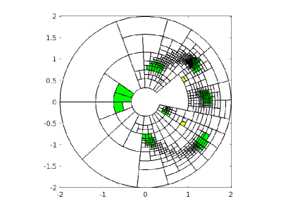
Refer to caption
Refer to caption
Figure 10: (a) There are no bifurcations taking place inside 𝒞1subscript𝒞1{\mathcal{C}}_{1}. For all parameters in 𝒫3subscript𝒫3{\mathcal{P}}_{3}, there exist seven solutions here, each located in one of the green connected regions. (b) Inside 𝒞2subscript𝒞2{\mathcal{C}}_{2} two kinds of bifurcations occur: quadratic and cubic. As before, some exclusion theorems are valid in the yellow sections.

The second part of the run focuses on the remaining portion of the configuration space 𝒞2subscript𝒞2{\mathcal{C}}_{2} (named 𝙲𝟶𝙲𝟶{\bf\tt C0} in the output); in polar coordinates 𝒞2=[13,1]×[210,710]subscript𝒞2131210710{\mathcal{C}}_{2}=[\tfrac{1}{3},1]\times[\tfrac{2}{10},\tfrac{7}{10}]. Throughout these computations, the parameter region 𝒫3subscript𝒫3{\mathcal{P}}_{3} is adaptively bisected into many smaller sets; each one being examined via various test. When successfully classified, a parameter set is stored in one of several lists. Together with each such parameter set, we also store a covering of all possible solutions in 𝒞2subscript𝒞2{\mathcal{C}}_{2}. The lists are organized as follows:

  • 1.

    s0List: the parameters are unordered (we do not consider these).

  • 2.

    s1List: the number of solutions is at most one and fixed (no bifurcations) in 𝒞2subscript𝒞2{\mathcal{C}}_{2}.

  • 3.

    s111List: there are three connected components in 𝒞2subscript𝒞2{\mathcal{C}}_{2}; in each one of them the number of solutions is at most one and fixed (no bifurcations).

  • 4.

    s210List: there are two connected components in 𝒞2subscript𝒞2{\mathcal{C}}_{2} where solutions may reside. For one of these the number of solutions is at most one and fixed (no bifurcations). For the second component there can be 0, 1, or 2 solutions (a quadratic bifurcation).

  • 5.

    s300List: there is one connected component in 𝒞2subscript𝒞2{\mathcal{C}}_{2} where the number of solutions can be 1, 2 or 3 (a cubic bifurcation).

We also mention that s3List is the union of s111List, s210List, and s300List.

Our final computation deals with the region (s,t)[0.25,0.5]×[0.55,0.58]𝑠𝑡0.250.50.550.58(s,t)\in[0.25,0.5]\times[0.55,0.58]:

$ ./pcr4bp 1e-6 0.25 0.50 0.55 0.58 3

============================================================
========================== pcr4bp ==========================
Started computations: Tue Mar 22 09:46:11 2022

Stopping tolerance in the search: TOL = +1.000000e-06
Parameter range for s = [+2.500000e-01, +5.000000e-01]
Parameter range for t = [+5.500000e-01, +5.800000e-01]
  This corresponds to
  m1 = [+1.375000e-01, +2.900000e-01]
  m2 = [+2.750000e-01, +4.350000e-01]
  m3 = [+4.200000e-01, +4.500000e-01]
=========================================================
Using strategy #3: Doing a full bifurcation analysis for
the entire parameter region.
=========================================================
Searching the following three outer regions of configuration space:
  C1 = {[+3.333333e-01, +2.000000e+00],[+7.000000e-01, +3.141593e+00]}
  C2 = {[+3.333333e-01, +2.000000e+00],[-3.141593e+00, -2.000000e-01]}
  C3 = {[+1.000000e+00, +2.000000e+00],[-2.000000e-01, +7.000000e-01]}
After bisection/determinant stage:
  unordered masses: +0
  |smallList|     : +0
  |noList|        : +1922
  |ndgList|       : +526
  |ndtList|       : +10
=========================================================
SUCCESS: the outer bifurcation analysis was conclusive.
There are no bifurcations occurring for these parameters.
=========================================================
Searching the single, inner region of configuration space:
  C0 = {[+3.333333e-01, +1.000000e+00],[-2.000000e-01, +7.000000e-01]}
Splitting tolerances for parameters: [+1.000000e-08, +5.000000e-02].
After the bisection/bifurcation stage:
  |smallList|: +0
  |s0List|   : +6
  |s1List|   : +149
  |s2List|   : +0
  |s3List|   : +253
  |s111List| : +103
  |s210List| : +150
  |s300List| : +0
There are subregions of C0 with at most three solutions.
There are subregions of C0 with at most one solution.
NOTE: we encountered regions in parameter space that
correspond to unordered masses. These were not analyzed.
=========================================================
SUCCESS: the inner bifurcation analysis was conclusive.
=========================================================
Ended computations: Tue Mar 22 09:46:53 2022
=========================================================

The main difference to the previous run, is that there are no cubic bifurcations in this parameter region; only quadratic. Indeed, s300List is empty, but s210List is not.

In summary, the classifications of the parameter sets corresponding to the lists produced by these three runs are illustrated in Figure 11.

Refer to caption
Figure 11: The bifurcations (and non-bifurcations) taking place within the parameter region 𝒫3=[0,0.5]×[0.55,0.58]subscript𝒫300.50.550.58{\mathcal{P}}_{3}=[0,0.5]\times[0.55,0.58]. There are five groups of parameters illustrated here: 1. the white region corresponds to s0List; 2. the green region corresponds to s1List; 3. the yellow region corresponds to s111List; 4. the blue region corresponds to s210List; 5. the red region corresponds to s300List. Each group of parameters forms a simply connected set.

The data presented in Figure 11 (and Figure 12) combined with our previous results provide all information needed to get an accurate count on the number of solutions.

First, note that the parameters in s1List form a connected set having a non-empty intersection with 𝒫1subscript𝒫1{\mathcal{P}}_{1}. We can therefore use part (a) of Theorem 8 to conclude that each parameter in s1List will yield exactly eight solutions in 𝒞𝒞{\mathcal{C}}: seven in 𝒞1subscript𝒞1{\mathcal{C}}_{1} and one in 𝒞2subscript𝒞2{\mathcal{C}}_{2}.

Similarly, we note that the parameters in s111List form a connected set having a non-empty intersection with 𝒫2subscript𝒫2{\mathcal{P}}_{2}. Using part (b) of Theorem 8 we conclude that out of the ten solutions in 𝒞𝒞{\mathcal{C}}, seven reside in 𝒞1subscript𝒞1{\mathcal{C}}_{1} and the remaining three belong to 𝒞2subscript𝒞2{\mathcal{C}}_{2}.

Turning to s210List, these parameters form a connected set having a non-empty intersection with both s1List and s111List. The bifurcation-free connected component of 𝒞2subscript𝒞2{\mathcal{C}}_{2} detected for all parameters in s210List must, by continuity, carry exactly one solution in 𝒞2subscript𝒞2{\mathcal{C}}_{2}. Thus each parameter in s210List yields 1, 2 or 3 solutions in 𝒞2subscript𝒞2{\mathcal{C}}_{2}.

Refer to caption
Refer to caption
Figure 12: Successive zoom-ins toward the region of finest subdivision in Figure 11.

Finally, we discuss the parameters in s300List. Without additional information, the condition used to indicate the presence of a cubic bifurcation does not exclude there being no solutions; it only bounds the number of solutions from above by three. We do, however, guarantee the existence of at least one solution for elements of s300List via an extra topological check performed during the computations.

As mentioned above, each parameter set stored in s300List comes equipped with a cover of the associated solution set {ci}i=1Nsuperscriptsubscriptsubscriptc𝑖𝑖1𝑁\{\textbf{{c}}_{i}\}_{i=1}^{N} making up a connected subset of 𝒞2subscript𝒞2{\mathcal{C}}_{2}. Forming the rectangular hull c of all cisubscriptc𝑖\textbf{{c}}_{i}, i=1,,N𝑖1𝑁i=1,\dots,N we prove that there must be a zero of f𝑓f inside c (and thus inside 𝒞2subscript𝒞2{\mathcal{C}}_{2}) using the following topological theorem.

Theorem 15.

Let f:[x,x+]×[y,y+]2:𝑓superscript𝑥superscript𝑥superscript𝑦superscript𝑦superscript2f\colon[x^{-},x^{+}]\times[y^{-},y^{+}]\to{\mathbb{R}}^{2} be a continuous function, and assume that the following holds:

  • 1.

    Both f1subscript𝑓1f_{1} and f2subscript𝑓2f_{2} are negative on the two sides {x}×[y,y+]superscript𝑥superscript𝑦superscript𝑦\{x^{-}\}\times[y^{-},y^{+}] and [x,x+]×{y}superscript𝑥superscript𝑥superscript𝑦[x^{-},x^{+}]\times\{y^{-}\}.

  • 2.

    Both f1subscript𝑓1f_{1} and f2subscript𝑓2f_{2} are positive at the upper-right corner (x+,y+)superscript𝑥superscript𝑦(x^{+},y^{+}).

  • 3.

    max{x[x,x+]:f1(x,y+)=0}<min{x[x,x+]:f2(x,y+)=0}:𝑥superscript𝑥superscript𝑥subscript𝑓1𝑥superscript𝑦0:𝑥superscript𝑥superscript𝑥subscript𝑓2𝑥superscript𝑦0\max\{x\in[x^{-},x^{+}]\colon f_{1}(x,y^{+})=0\}<\min\{x\in[x^{-},x^{+}]\colon f_{2}(x,y^{+})=0\}.

  • 4.

    max{y[y,y+]:f2(x+,y)=0}<min{y[y,y+]:f1(x+,y)=0}:𝑦superscript𝑦superscript𝑦subscript𝑓2superscript𝑥𝑦0:𝑦superscript𝑦superscript𝑦subscript𝑓1superscript𝑥𝑦0\max\{y\in[y^{-},y^{+}]\colon f_{2}(x^{+},y)=0\}<\min\{y\in[y^{-},y^{+}]\colon f_{1}(x^{+},y)=0\}.

Then f𝑓f has (at least) one zero in [x,x+]×[y,y+]superscript𝑥superscript𝑥superscript𝑦superscript𝑦[x^{-},x^{+}]\times[y^{-},y^{+}].

Of course, the theorem remains true when we reverse all appearing signs, or interchange the function components. We can also relax assumption 1 and simply demand that f1subscript𝑓1f_{1} is negative on [x,x+]×{y}superscript𝑥superscript𝑥superscript𝑦[x^{-},x^{+}]\times\{y^{-}\}, and f2subscript𝑓2f_{2} is negative on {x}×[y,y+]superscript𝑥superscript𝑦superscript𝑦\{x^{-}\}\times[y^{-},y^{+}]. We keep the current (stronger) assumptions as they actually hold for the problem at hand. A typical realization of these are illustrated in Figure 13.
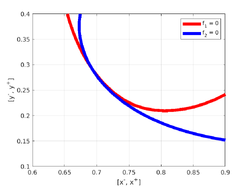
Refer to caption
Figure 13: An illustration of how the (set-valued) zero-sets of f1subscript𝑓1f_{1} and f2subscript𝑓2f_{2} behave for typical parameters in s300List.
Proof.

By the intermediate value theorem, assumptions 1 and 2 imply that both f1subscript𝑓1f_{1} and f2subscript𝑓2f_{2} change sign (and therefore vanish) somewhere along the two sides [x,x+]×{y+}superscript𝑥superscript𝑥superscript𝑦[x^{-},x^{+}]\times\{y^{+}\} and {x+}×[y,y+]superscript𝑥superscript𝑦superscript𝑦\{x^{+}\}\times[y^{-},y^{+}]. Therefore the sets appearing in assumptions 3 and 4 are non-empty, and the inequalities can be checked. Now, let xsuperscript𝑥x^{\star} satisfy max{x[x,x+]:f1(x,y+)=0}<x<min{x[x,x+]:f2(x,y+)=0}:𝑥superscript𝑥superscript𝑥subscript𝑓1𝑥superscript𝑦0superscript𝑥:𝑥superscript𝑥superscript𝑥subscript𝑓2𝑥superscript𝑦0\max\{x\in[x^{-},x^{+}]\colon f_{1}(x,y^{+})=0\}<x^{\star}<\min\{x\in[x^{-},x^{+}]\colon f_{2}(x,y^{+})=0\}. Similarly, let ysuperscript𝑦y^{\star} satisfy max{y[y,y+]:f2(x+,y)=0}<y<min{y[y,y+]:f1(x+,y)=0}:𝑦superscript𝑦superscript𝑦subscript𝑓2superscript𝑥𝑦0superscript𝑦:𝑦superscript𝑦superscript𝑦subscript𝑓1superscript𝑥𝑦0\max\{y\in[y^{-},y^{+}]\colon f_{2}(x^{+},y)=0\}<y^{\star}<\min\{y\in[y^{-},y^{+}]\colon f_{1}(x^{+},y)=0\}. Then, by a continuous deformation, we can form a new rectangle with corners (x,y),(x,y+),(x+,y+)superscript𝑥superscript𝑦superscript𝑥superscript𝑦superscript𝑥superscript𝑦(x^{-},y^{-}),(x^{\star},y^{+}),(x^{+},y^{+}), and (x+,y)superscript𝑥superscript𝑦(x^{+},y^{\star}) on which we can directly apply the Poincaré-Miranda theorem, see [9]. It follows that f𝑓f has a zero in the original rectangle. ∎

As all assumptions of the theorem are open, we can extend it to the case when f𝑓f depends on (set-valued) parameters. This is what we use for the parameters forming 𝚜𝟹𝟶𝟶𝙻𝚒𝚜𝚝𝚜𝟹𝟶𝟶𝙻𝚒𝚜𝚝{\bf\tt s300List}.

7.4 Timings

We end this section by reporting the timings of all computations. These we carried out sequencially on a latop, using a single thread on an Intel Core i7-7500U CPU running at 2.70GHz. The memory requirements are very low, and are not reported. For all computations we used the same splitting tolerance: 𝚝𝚘𝚕=106𝚝𝚘𝚕superscript106{\bf\tt tol}=10^{-6}. The total wall time amounts to 16m:29s. This can of course be massively reduced by a finer pre-splitting in parameter space, combined with a simple script for parallel execution.

sMin sMax tMin tMax strategy time
0.25 0.25 0.25 0.25 1 0m00s
0.45 0.45 0.60 0.60 1 0m00s
0.00 0.50 0.58 0.67 2 0m02s
0.00 1e-6 0.00 1e-6 2 0m01s
1e-6 0.50 0.00 1e-6 2 1m30s
0.00 1e-6 1e-6 0.55 2 7m40s
1e-6 0.50 1e-6 0.55 2 1m38s
0.00 0.20 0.55 0.58 3 0m02s
0.20 0.25 0.55 0.58 3 4m53s
0.25 0.50 0.55 0.58 3 0m43s
Table 1: Wall timings for the computer-assisted part of the proof.

8 Conclusions and future work

We have demonstrated a novel way to account for all relative equilibria in the planar, circular, restricted 4-body problem, and used it to give a new proof of the results by Barros and Leandro (Theorem 6). The novely of our approach is that it does not rely upon any algebraic considerations; it is purely analytic. As such it is completely insensitive to the exact shape of the gravitational potential, and generalizes to a wider range of problems. The main advantage, however, is that our method is amenable to set-valued computations, and as such can use the mature techniques and machinery available to solve non-linear equations with computer-assisted methods. This, in turn, gives us a realistic expectation that our approach is transferable to harder instances of the n𝑛n-body problem, and our next challenge will be to work on the unrestricted 4-body problem, where we expect the number of relative equilibria to range between 32 and 50 (depending on the masses of the four primaries).

9 Acknowledgments

We are very greatful to Professor Carles Simó for bringing this problem to our attention and for fruitful discussions. W. T. has been partially supported by VR grant 2013-4964. P. Z. has been partially supported by the NCN grant 2019/35/B/ST1/00655.

References

  • [1] A. Albouy and V. Kaloshin. Finiteness of central configurations of five bodies in the plane. Annals of Mathematics, 176:535–588, 2012.
  • [2] J. Barros and E. Leandro. The set of degenerate central configurations in the planar restricted four-body problem. SIAM J. Math. Analysis, 43:634–661, 01 2011.
  • [3] J. Barros and E. Leandro. Bifurcations and enumeration of classes of relative equilibria in the planar restricted four-body problem. SIAM Journal on Mathematical Analysis, 46, 03 2014.
  • [4] L. Euler. De motu rectilineo trium corporum se mutuo attrahentium. Novi Comm. Acad. Sci. Imp. Petrop., 11:144–151, 1767.
  • [5] M. Hampton and R. Moeckel. Finiteness of relative equilibria of the four-body problem. Inventiones Mathematicae, 163:289–312, 2006.
  • [6] R. Krawczyk. Newton-algorithmen zur besstimmung von nullstellen mit fehlerschranken. Computing, 4:187–201, 1969.
  • [7] J. Kulevich, G. Roberts, and C. Smith. Finiteness in the planar restricted four-body problem. Qualitative Theory of Dynamical Systems, 8:357–370, 12 2010.
  • [8] J.L. Lagrange. Essai sur le problème des trois corps. Oevres, 6:229–324, 1772.
  • [9] C. Miranda. Un’osservazione su un teorema di Brouwer. Consiglio Nazionale delle Ricerche, 1940.
  • [10] F.R. Moulton. The straight line solutions of the problem of n𝑛n bodies. Annals of Mathematics, 12:1–17, 1910.
  • [11] A. Neumaier. Interval Methods for Systems of Equations. Cambridge University Press, 1990.
  • [12] G.E. Roberts. A continuum of relative equilibria in the five-body problem. Physica D: Nonlinear Phenomena, 127(3:4):141–145, 1999.
  • [13] C. Simó. Relative equilibrium solutions in the four body problem. Celestial Mechanics, 18:165–184, 1978.
  • [14] W. Tucker. Validated Numerics: A Short Introduction to Rigorous Computations. Princeton University Press, 2011.

Appendix A Bounding the number of small masses

The goal of this appendix is to prove Theorem 13.

From the discussion in Section 2.2 (see (4)) we know that that no relative equilibrium exist close to p3subscript𝑝3p_{3}, while for small m1subscript𝑚1m_{1} or m2subscript𝑚2m_{2} the relative equilibria can exists arbitrarily close to p1subscript𝑝1p_{1} and p2subscript𝑝2p_{2} (this is proved in this appendix). If we relax the requirement that m1m2subscript𝑚1subscript𝑚2m_{1}\leq m_{2}, then it is enough to investigate the neighborhood of p1subscript𝑝1p_{1} and the same conclusions will be valid by symmetry close to p2subscript𝑝2p_{2}.

We will investigate the neighborhood of p1subscript𝑝1p_{1} when m1(0,M]subscript𝑚10𝑀m_{1}\in(0,M] and 0<m2<10subscript𝑚210<m_{2}<1 with M=102𝑀superscript102M=10^{-2}. This will be split later in two cases: when the second mass m2subscript𝑚2m_{2} is away from zero (m2M=102subscript𝑚2𝑀superscript102m_{2}\geq M=10^{-2}) and when m2[0,M]subscript𝑚20𝑀m_{2}\in[0,M]. The difference between these two cases is that for the former we can control all (four) the solutions in a neighbourhood of p1subscript𝑝1p_{1}, while in the latter two of the four can escape the neighbourhood (while the other two stay always in it). Technically this is related to the behaviour of the eigenvalues of Hessian of the nonsingular part of V𝑉V at p1subscript𝑝1p_{1}. In the first case both eigenvalues are separated from 00 and the second case the smaller eigenvalue approaches zero when m1,m20subscript𝑚1subscript𝑚20m_{1},m_{2}\to 0.

A.1 The separation of eigenvalues at p1subscript𝑝1p_{1} for non-singular part of V𝑉V

Let

V~(x,y)=V(p1+(x,y))m1zp1=12DV~(p1)((x,y),(x,y))+O((x,y)3).~𝑉𝑥𝑦𝑉subscript𝑝1𝑥𝑦subscript𝑚1norm𝑧subscript𝑝112𝐷~𝑉subscript𝑝1𝑥𝑦𝑥𝑦𝑂superscriptnorm𝑥𝑦3\widetilde{V}(x,y)=V(p_{1}+(x,y))-\frac{m_{1}}{\|z-p_{1}\|}=\frac{1}{2}D\tilde{V}(p_{1})((x,y),(x,y))+O(\|(x,y)\|^{3}). (31)

The following straightforward lemma will be used during the entire discussion.

Lemma 16.

The matrix DV~(p1)𝐷~𝑉subscript𝑝1D\tilde{V}(p_{1}) is positive definite. Moreover, if m11/2subscript𝑚112m_{1}\leq 1/2 (in our case it is true because m3m1subscript𝑚3subscript𝑚1m_{3}\geq m_{1} and m3+m11subscript𝑚3subscript𝑚11m_{3}+m_{1}\leq 1), then its eigenvalues λ1>λ2subscript𝜆1subscript𝜆2\lambda_{1}>\lambda_{2} are given by

λ1,2subscript𝜆12\displaystyle\lambda_{1,2} =\displaystyle= 12(2+m2+m3±3m22m2m3+m32)=12plus-or-minus2subscript𝑚2subscript𝑚33superscriptsubscript𝑚22subscript𝑚2subscript𝑚3superscriptsubscript𝑚32absent\displaystyle\frac{1}{2}\left(2+m_{2}+m_{3}\pm 3\sqrt{m_{2}^{2}-m_{2}m_{3}+m_{3}^{2}}\right)= (32)
=\displaystyle= 12(2+m2+m3±3(m2+m3)23m2m3),12plus-or-minus2subscript𝑚2subscript𝑚33superscriptsubscript𝑚2subscript𝑚323subscript𝑚2subscript𝑚3\displaystyle\frac{1}{2}\left(2+m_{2}+m_{3}\pm 3\sqrt{(m_{2}+m_{3})^{2}-3m_{2}m_{3}}\right),

and satisfy the following inequalities

m1+9m2m32(m2+m3)subscript𝑚19subscript𝑚2subscript𝑚32subscript𝑚2subscript𝑚3\displaystyle m_{1}+\frac{9m_{2}m_{3}}{2(m_{2}+m_{3})} >\displaystyle> λ2>m1+9m2m34(m2+m3),subscript𝜆2subscript𝑚19subscript𝑚2subscript𝑚34subscript𝑚2subscript𝑚3\displaystyle\lambda_{2}>m_{1}+\frac{9m_{2}m_{3}}{4(m_{2}+m_{3})},
λ1subscript𝜆1\displaystyle\lambda_{1} <\displaystyle< 3,3\displaystyle 3,
3434\displaystyle\frac{3}{4} \displaystyle\leq λ1λ2<3.subscript𝜆1subscript𝜆23\displaystyle\lambda_{1}-\lambda_{2}<3.

The proof of this lemma is straightforward. It is important to notice that if m1,m20subscript𝑚1subscript𝑚20m_{1},m_{2}\to 0, then λ20subscript𝜆20\lambda_{2}\to 0, but if m2>ϵsubscript𝑚2italic-ϵm_{2}>\epsilon then λ2subscript𝜆2\lambda_{2} stays away from 00. Also that λ1λ2subscript𝜆1subscript𝜆2\lambda_{1}-\lambda_{2} has a positive lower bound independent of the size of m1subscript𝑚1m_{1} and m2subscript𝑚2m_{2}. Moreover, with the help of the code Bounds_eigenvalues and under the assumption that m2,m3102subscript𝑚2subscript𝑚3superscript102m_{2},m_{3}\geq 10^{-2} we can obtain sharper bounds: λ1λ2<2.95643subscript𝜆1subscript𝜆22.95643\lambda_{1}-\lambda_{2}<2.95643, 1.62287<λ1<2.978431.62287subscript𝜆12.978431.62287<\lambda_{1}<2.97843, 0.02167<λ2<0.876950.02167subscript𝜆20.876950.02167<\lambda_{2}<0.87695. Also, if we allow m2,m3[0,1]subscript𝑚2subscript𝑚301m_{2},m_{3}\in[0,1] then we have λ1[1,3]subscript𝜆113\lambda_{1}\in[1,3] and λ2[0,1]subscript𝜆201\lambda_{2}\in[0,1].

A.2 Estimates for higher order terms in V𝑉V

We shift the coordinate origin to p1subscript𝑝1p_{1}. Then V(x,y)𝑉𝑥𝑦V(x,y) can be written as follows

V(x,y)=m1r+V~(0,0)+DV~(x,y)+h(x,y),𝑉𝑥𝑦subscript𝑚1𝑟~𝑉00𝐷~𝑉𝑥𝑦𝑥𝑦V(x,y)=\frac{m_{1}}{r}+\tilde{V}(0,0)+D\tilde{V}(x,y)+h(x,y), (33)

where r=(x,y)𝑟norm𝑥𝑦r=\|(x,y)\| and hh is analytic with respect to all variables and is O((x,y)3)𝑂superscriptnorm𝑥𝑦3O(\|(x,y)\|^{3}) uniformly with respect to the masses. In fact hh depends linearly on masses m2subscript𝑚2m_{2} and m3subscript𝑚3m_{3}. The term V(0,0)𝑉00V(0,0) will be ignored.

For any R>0𝑅0R>0 there exist C1=C1(m2,m3,x,y)subscript𝐶1subscript𝐶1subscript𝑚2subscript𝑚3𝑥𝑦C_{1}=C_{1}(m_{2},m_{3},x,y) and C2=C2(m2,m3,x,y)subscript𝐶2subscript𝐶2subscript𝑚2subscript𝑚3𝑥𝑦C_{2}=C_{2}(m_{2},m_{3},x,y) such that

(x,y)h(x,y)normsubscript𝑥𝑦𝑥𝑦\displaystyle\left\|\nabla_{(x,y)}h(x,y)\right\| <\displaystyle< C1(x,y)2,subscript𝐶1superscriptnorm𝑥𝑦2\displaystyle C_{1}\|(x,y)\|^{2}, (34)
D(x,y)2h(x,y)normsuperscriptsubscript𝐷𝑥𝑦2𝑥𝑦\displaystyle\left\|D_{(x,y)}^{2}h(x,y)\right\| <\displaystyle< C2(x,y).subscript𝐶2norm𝑥𝑦\displaystyle C_{2}\|(x,y)\|. (35)

for (x,y)Rnorm𝑥𝑦𝑅\|(x,y)\|\leq R.

We obtain quantitative instances of the upper bounds (34) and (35) as follows: we set R=2𝑅2R=2 (from the discussion in Section A.1 it follows that for any i=1,2,3𝑖123i=1,2,3 all relative equilibria are contained in B¯(pi,R)¯𝐵subscript𝑝𝑖𝑅\overline{B}(p_{i},R).) By performing automatic differentiation of the function h(x,y)𝑥𝑦h(x,y) for all (x,y)𝑥𝑦(x,y) with (x,y)104norm𝑥𝑦superscript104\|(x,y)\|\leq 10^{-4}, the first one is three times the sum of all Taylor coefficients of order 3, and the second one is six times the sum of all Taylor coefficients of order 3. Hence, using the code Bounds_h and under the assumption of 0m2,m31formulae-sequence0subscript𝑚2subscript𝑚310\leq m_{2},m_{3}\leq 1, and (x,y)103norm𝑥𝑦superscript103\|(x,y)\|\leq 10^{-3}, we obtain the bounds

C19.68850,C219.3770.formulae-sequencesubscript𝐶19.68850subscript𝐶219.3770C_{1}\leq 9.68850,\qquad C_{2}\leq 19.3770. (36)

A.2.1 Estimates in polar coordinates

Using the polar coordinates we obtain the following expressions for partial derivatives of h(r,φ)𝑟𝜑h(r,\varphi)

hr(r,φ)𝑟𝑟𝜑\displaystyle\frac{\partial h}{\partial r}(r,\varphi) =\displaystyle= hx(rcosφ,rsinφ)cosφ+hy(rcosφ,rsinφ)sinφ,𝑥𝑟𝜑𝑟𝜑𝜑𝑦𝑟𝜑𝑟𝜑𝜑\displaystyle\frac{\partial h}{\partial x}(r\cos\varphi,r\sin\varphi)\cos\varphi+\frac{\partial h}{\partial y}(r\cos\varphi,r\sin\varphi)\sin\varphi,
hφ(r,φ)𝜑𝑟𝜑\displaystyle\frac{\partial h}{\partial\varphi}(r,\varphi) =\displaystyle= r(hxsinφ+hycosφ),𝑟𝑥𝜑𝑦𝜑\displaystyle r\left(-\frac{\partial h}{\partial x}\sin\varphi+\frac{\partial h}{\partial y}\cos\varphi\right),
2hr2(r,φ)superscript2superscript𝑟2𝑟𝜑\displaystyle\frac{\partial^{2}h}{\partial r^{2}}(r,\varphi) =\displaystyle= 2hx2cos2φ+22hxysinφcosφ+2hy2sin2φ,superscript2superscript𝑥2superscript2𝜑2superscript2𝑥𝑦𝜑𝜑superscript2superscript𝑦2superscript2𝜑\displaystyle\frac{\partial^{2}h}{\partial x^{2}}\cos^{2}\varphi+2\frac{\partial^{2}h}{\partial x\partial y}\sin\varphi\cos\varphi+\frac{\partial^{2}h}{\partial y^{2}}\sin^{2}\varphi,
2hrφ(r,φ)superscript2𝑟𝜑𝑟𝜑\displaystyle\frac{\partial^{2}h}{\partial r\partial\varphi}(r,\varphi) =\displaystyle= (hxsinφ+hycosφ)+limit-from𝑥𝜑𝑦𝜑\displaystyle\left(-\frac{\partial h}{\partial x}\sin\varphi+\frac{\partial h}{\partial y}\cos\varphi\right)+
r((2hx2+2hy2)sinφcosφ+2hxy(cos2φsin2φ)),𝑟superscript2superscript𝑥2superscript2superscript𝑦2𝜑𝜑superscript2𝑥𝑦superscript2𝜑superscript2𝜑\displaystyle r\left(\left(-\frac{\partial^{2}h}{\partial x^{2}}+\frac{\partial^{2}h}{\partial y^{2}}\right)\sin\varphi\cos\varphi+\frac{\partial^{2}h}{\partial x\partial y}(\cos^{2}\varphi-\sin^{2}\varphi)\right),
2hφ2(r,φ)superscript2superscript𝜑2𝑟𝜑\displaystyle\frac{\partial^{2}h}{\partial\varphi^{2}}(r,\varphi) =\displaystyle= r(hxcosφ+hysinφ)+limit-from𝑟𝑥𝜑𝑦𝜑\displaystyle-r\left(\frac{\partial h}{\partial x}\cos\varphi+\frac{\partial h}{\partial y}\sin\varphi\right)+
r2(2hx2sin2φ22hxysinφcosφ+2hy2cos2φ).superscript𝑟2superscript2superscript𝑥2superscript2𝜑2superscript2𝑥𝑦𝜑𝜑superscript2superscript𝑦2superscript2𝜑\displaystyle r^{2}\left(\frac{\partial^{2}h}{\partial x^{2}}\sin^{2}\varphi-2\frac{\partial^{2}h}{\partial x\partial y}\sin\varphi\cos\varphi+\frac{\partial^{2}h}{\partial y^{2}}\cos^{2}\varphi\right).

Let

e=(cosφ,sinφ),e=(sinφ,cosφ).formulae-sequence𝑒𝜑𝜑superscript𝑒bottom𝜑𝜑e=(\cos\varphi,\sin\varphi),\quad e^{\bot}=(-\sin\varphi,\cos\varphi).

In a more geometric way we can express the above partial derivatives as follows

hr(r,φ)𝑟𝑟𝜑\displaystyle\frac{\partial h}{\partial r}(r,\varphi) =\displaystyle= (h,e),𝑒\displaystyle(\nabla h,e),
hφ(r,φ)𝜑𝑟𝜑\displaystyle\frac{\partial h}{\partial\varphi}(r,\varphi) =\displaystyle= r(h,e),𝑟superscript𝑒bottom\displaystyle r(\nabla h,e^{\bot}),
2hr2(r,φ)superscript2superscript𝑟2𝑟𝜑\displaystyle\frac{\partial^{2}h}{\partial r^{2}}(r,\varphi) =\displaystyle= D2h(e,e),superscript𝐷2𝑒𝑒\displaystyle D^{2}h(e,e),
2hrφ(r,φ)superscript2𝑟𝜑𝑟𝜑\displaystyle\frac{\partial^{2}h}{\partial r\partial\varphi}(r,\varphi) =\displaystyle= (h,e)+rD2h(e,e),superscript𝑒bottom𝑟superscript𝐷2superscript𝑒bottom𝑒\displaystyle(\nabla h,e^{\bot})+rD^{2}h(e^{\bot},e),
2hφ2(r,φ)superscript2superscript𝜑2𝑟𝜑\displaystyle\frac{\partial^{2}h}{\partial\varphi^{2}}(r,\varphi) =\displaystyle= r(h,e)+r2D2h(e,e).𝑟𝑒superscript𝑟2superscript𝐷2superscript𝑒bottomsuperscript𝑒bottom\displaystyle-r(\nabla h,e)+r^{2}D^{2}h(e^{\bot},e^{\bot}).

Therefore we have the following estimates for the partial derivatives of hh with respect to polar coordinates.

Lemma 17.

Assume that (34,35) hold for rR𝑟𝑅r\leq R. Then the following estimates are satisfied for rR𝑟𝑅r\leq R

|hr(r,φ)|𝑟𝑟𝜑\displaystyle\left|\frac{\partial h}{\partial r}(r,\varphi)\right| <\displaystyle< C1r2,subscript𝐶1superscript𝑟2\displaystyle C_{1}r^{2},
|hφ(r,φ)|𝜑𝑟𝜑\displaystyle\left|\frac{\partial h}{\partial\varphi}(r,\varphi)\right| <\displaystyle< C1r3,subscript𝐶1superscript𝑟3\displaystyle C_{1}r^{3},
|2hr2(r,φ)|superscript2superscript𝑟2𝑟𝜑\displaystyle\left|\frac{\partial^{2}h}{\partial r^{2}}(r,\varphi)\right| <\displaystyle< C2r,subscript𝐶2𝑟\displaystyle C_{2}r,
|2hrφ(r,φ)|superscript2𝑟𝜑𝑟𝜑\displaystyle\left|\frac{\partial^{2}h}{\partial r\partial\varphi}(r,\varphi)\right| <\displaystyle< C1r2+C2r2=(C1+C2)r2,subscript𝐶1superscript𝑟2subscript𝐶2superscript𝑟2subscript𝐶1subscript𝐶2superscript𝑟2\displaystyle C_{1}r^{2}+C_{2}r^{2}=(C_{1}+C_{2})r^{2},
|2hφ2(r,φ)|superscript2superscript𝜑2𝑟𝜑\displaystyle\left|\frac{\partial^{2}h}{\partial\varphi^{2}}(r,\varphi)\right| <\displaystyle< C1r3+C2r3=(C1+C2)r3.subscript𝐶1superscript𝑟3subscript𝐶2superscript𝑟3subscript𝐶1subscript𝐶2superscript𝑟3\displaystyle C_{1}r^{3}+C_{2}r^{3}=(C_{1}+C_{2})r^{3}.
Lemma 18.

The same assumptions as in Lemma 17. Let us set

h~φ(r,φ)subscript~𝜑𝑟𝜑\displaystyle\tilde{h}_{\varphi}(r,\varphi) =\displaystyle= 1r3hφ(r,φ),1superscript𝑟3𝜑𝑟𝜑\displaystyle\frac{1}{r^{3}}\frac{\partial h}{\partial\varphi}(r,\varphi),
h~φφ(r,φ)subscript~𝜑𝜑𝑟𝜑\displaystyle\tilde{h}_{\varphi\varphi}(r,\varphi) =\displaystyle= 1r32hφ2(r,φ),1superscript𝑟3superscript2superscript𝜑2𝑟𝜑\displaystyle\frac{1}{r^{3}}\frac{\partial^{2}h}{\partial\varphi^{2}}(r,\varphi),
h~φr(r,φ)subscript~𝜑𝑟𝑟𝜑\displaystyle\tilde{h}_{\varphi r}(r,\varphi) =\displaystyle= 1r22hφr(r,φ),1superscript𝑟2superscript2𝜑𝑟𝑟𝜑\displaystyle\frac{1}{r^{2}}\frac{\partial^{2}h}{\partial\varphi\partial r}(r,\varphi),
h~r(r,φ)subscript~𝑟𝑟𝜑\displaystyle\tilde{h}_{r}(r,\varphi) =\displaystyle= 1r2hr(r,φ),1superscript𝑟2𝑟𝑟𝜑\displaystyle\frac{1}{r^{2}}\frac{\partial h}{\partial r}(r,\varphi),
h~rr(r,φ)subscript~𝑟𝑟𝑟𝜑\displaystyle\tilde{h}_{rr}(r,\varphi) =\displaystyle= 1r2hr2(r,φ).1𝑟superscript2superscript𝑟2𝑟𝜑\displaystyle\frac{1}{r}\frac{\partial^{2}h}{\partial r^{2}}(r,\varphi).

Then we have for rR𝑟𝑅r\leq R

|h~φ(r,φ)|<C1,|h~φφ(r,φ)|<C1+C2,|h~φr(r,φ)|<C1+C2formulae-sequencesubscript~𝜑𝑟𝜑subscript𝐶1formulae-sequencesubscript~𝜑𝜑𝑟𝜑subscript𝐶1subscript𝐶2subscript~𝜑𝑟𝑟𝜑subscript𝐶1subscript𝐶2\displaystyle|\tilde{h}_{\varphi}(r,\varphi)|<C_{1},\quad|\tilde{h}_{\varphi\varphi}(r,\varphi)|<C_{1}+C_{2},\quad|\tilde{h}_{\varphi r}(r,\varphi)|<C_{1}+C_{2} (37)
|h~r(r,φ)|<C1,|h~rr(r,φ)|<C2formulae-sequencesubscript~𝑟𝑟𝜑subscript𝐶1subscript~𝑟𝑟𝑟𝜑subscript𝐶2\displaystyle|\tilde{h}_{r}(r,\varphi)|<C_{1},\quad|\tilde{h}_{rr}(r,\varphi)|<C_{2} (38)

A.3 Our system in polar coordinates near p1subscript𝑝1p_{1}

By an orthogonal change of variables V𝑉V we can diagonalize DV~(0)𝐷~𝑉0D\widetilde{V}(0), hence V𝑉V can be written as follows (compare (33))

V(x,y)=m1r+λx22+ay22+h(x,y).𝑉𝑥𝑦subscript𝑚1𝑟𝜆superscript𝑥22𝑎superscript𝑦22𝑥𝑦V(x,y)=\frac{m_{1}}{r}+\lambda\frac{x^{2}}{2}+a\frac{y^{2}}{2}+h(x,y). (39)

Observe that λ𝜆\lambda and a𝑎a depend on mass parameters (see Lemma 16) and the same holds for the coordinate change. Bounds on hh and its derivatives uniform with respect to masses have been obtained for r<R𝑟𝑅r<R in previous subsections.

In polar coordinates our potential (39) becomes (we set m=m1𝑚subscript𝑚1m=m_{1})

V(r,φ)=mr+ar22+(λa)r2cos2φ2+h(r,φ)𝑉𝑟𝜑𝑚𝑟𝑎superscript𝑟22𝜆𝑎superscript𝑟2superscript2𝜑2𝑟𝜑V(r,\varphi)=\frac{m}{r}+\frac{ar^{2}}{2}+\frac{(\lambda-a)r^{2}\cos^{2}\varphi}{2}+h(r,\varphi) (40)

and

Vr(r,φ)𝑉𝑟𝑟𝜑\displaystyle\frac{\partial V}{\partial r}(r,\varphi) =\displaystyle= mr2+ar+(λa)rcos2φ+hr(r,φ)=𝑚superscript𝑟2𝑎𝑟𝜆𝑎𝑟superscript2𝜑𝑟𝑟𝜑absent\displaystyle-\frac{m}{r^{2}}+ar+(\lambda-a)r\cos^{2}\varphi+\frac{\partial h}{\partial r}(r,\varphi)= (41)
=\displaystyle= mr2+r(λ+a2+λa2cos(2φ))+r2h~r,𝑚superscript𝑟2𝑟𝜆𝑎2𝜆𝑎22𝜑superscript𝑟2subscript~𝑟\displaystyle-\frac{m}{r^{2}}+r\left(\frac{\lambda+a}{2}+\frac{\lambda-a}{2}\cos(2\varphi)\right)+r^{2}\tilde{h}_{r},
Vφ(r,φ)𝑉𝜑𝑟𝜑\displaystyle\frac{\partial V}{\partial\varphi}(r,\varphi) =\displaystyle= (λa)r2sin(2φ)/2+hφ(r,φ)=𝜆𝑎superscript𝑟22𝜑2𝜑𝑟𝜑absent\displaystyle-(\lambda-a)r^{2}\sin(2\varphi)/2+\frac{\partial h}{\partial\varphi}(r,\varphi)=
=\displaystyle= (λa)r2sin(2φ)/2+r3h~φ(r,φ)=𝜆𝑎superscript𝑟22𝜑2superscript𝑟3subscript~𝜑𝑟𝜑absent\displaystyle-(\lambda-a)r^{2}\sin(2\varphi)/2+r^{3}\tilde{h}_{\varphi}(r,\varphi)=
=\displaystyle= r2((λa)sin(2φ)/2+rh~φ(r,φ)),superscript𝑟2𝜆𝑎2𝜑2𝑟subscript~𝜑𝑟𝜑\displaystyle r^{2}\left(-(\lambda-a)\sin(2\varphi)/2+r\tilde{h}_{\varphi}(r,\varphi)\right),
2Vr2(r,φ)superscript2𝑉superscript𝑟2𝑟𝜑\displaystyle\frac{\partial^{2}V}{\partial r^{2}}(r,\varphi) =\displaystyle= 2mr3+λ+a2+λa2cos(2φ)+2hr2(r,φ)2𝑚superscript𝑟3𝜆𝑎2𝜆𝑎22𝜑superscript2superscript𝑟2𝑟𝜑\displaystyle\frac{2m}{r^{3}}+\frac{\lambda+a}{2}+\frac{\lambda-a}{2}\cos(2\varphi)+\frac{\partial^{2}h}{\partial r^{2}}(r,\varphi) (43)
2Vφ2(r,φ)superscript2𝑉superscript𝜑2𝑟𝜑\displaystyle\frac{\partial^{2}V}{\partial\varphi^{2}}(r,\varphi) =\displaystyle= (λa)r2cos(2φ)+2hφ2(r,φ)=𝜆𝑎superscript𝑟22𝜑superscript2superscript𝜑2𝑟𝜑absent\displaystyle-(\lambda-a)r^{2}\cos(2\varphi)+\frac{\partial^{2}h}{\partial\varphi^{2}}(r,\varphi)= (44)
=\displaystyle= r2((λa)cos(2φ)+rh~φφ(r,φ)),superscript𝑟2𝜆𝑎2𝜑𝑟subscript~𝜑𝜑𝑟𝜑\displaystyle r^{2}\left(-(\lambda-a)\cos(2\varphi)+r\tilde{h}_{\varphi\varphi}(r,\varphi)\right),
2Vφr(r,φ)superscript2𝑉𝜑𝑟𝑟𝜑\displaystyle\frac{\partial^{2}V}{\partial\varphi\partial r}(r,\varphi) =\displaystyle= (λa)rsin(2φ)+2hrφ.𝜆𝑎𝑟2𝜑superscript2𝑟𝜑\displaystyle-(\lambda-a)r\sin(2\varphi)+\frac{\partial^{2}h}{\partial r\partial\varphi}. (45)

We will study the system

Vφ(r,φ)𝑉𝜑𝑟𝜑\displaystyle\frac{\partial V}{\partial\varphi}(r,\varphi) =\displaystyle= 0,0\displaystyle 0, (46)
Vr(r,φ)𝑉𝑟𝑟𝜑\displaystyle\frac{\partial V}{\partial r}(r,\varphi) =\displaystyle= 0.0\displaystyle 0. (47)

It turns out that it is relatively easy to solve (46), i.e. to find four curves φ(r)𝜑𝑟\varphi(r) such that all solutions of (46) are of the form (r,φ(r))𝑟𝜑𝑟(r,\varphi(r)). This is done in the next subsection for 0<m2<10subscript𝑚210<m_{2}<1 and m1subscript𝑚1m_{1} small enough.

Then we study the equation Vr(r,φ(r))=0𝑉𝑟𝑟𝜑𝑟0\frac{\partial V}{\partial r}(r,\varphi(r))=0 on each of these curves. This is the place where we will split our considerations into two cases: m2subscript𝑚2m_{2} bounded from below and both m1,m20subscript𝑚1subscript𝑚20m_{1},m_{2}\to 0. The second case is much more subtle.

A.4 Solving Vφ(r,φ)=0𝑉𝜑𝑟𝜑0\frac{\partial V}{\partial\varphi}(r,\varphi)=0 for φ(r)𝜑𝑟\varphi(r).

Our strategy to study the solutions of Vφ(r,φ(r))=0𝑉𝜑𝑟𝜑𝑟0\frac{\partial V}{\partial\varphi}(r,\varphi(r))=0 in the set {(r,φ):rR,φ[0,2π]}conditional-set𝑟𝜑formulae-sequence𝑟𝑅𝜑02𝜋\{(r,\varphi):r\leq R,\varphi\in[0,2\pi]\} is: we try to find possible large intervals such that the solution is excluded, for this it is enough to have (see (A.3) and Lemma 18)

(λa)|sin(2φ)|/2RC1,𝜆𝑎2𝜑2𝑅subscript𝐶1(\lambda-a)|\sin(2\varphi)|/2\geq RC_{1}, (48)

and then on the complementary intervals we want 2Vφ2superscript2𝑉superscript𝜑2\frac{\partial^{2}V}{\partial\varphi^{2}} to be either positive or negative on the whole interval, this is guaranteed by the following inequality (see (44)) and Lemma 18)

(λa)|cos(2φ)|R(C1+C2).𝜆𝑎2𝜑𝑅subscript𝐶1subscript𝐶2(\lambda-a)|\cos(2\varphi)|\geq R(C_{1}+C_{2}). (49)
Remark 19.

Recall that all this computations must have R2𝑅2R\leq 2 since this is the range where the existence of the constants C1,C2subscript𝐶1subscript𝐶2C_{1},C_{2} have been proved.

To deal with (48) let us set

α=arcsin(2RC1λa)(0,π/2).𝛼2𝑅subscript𝐶1𝜆𝑎0𝜋2\alpha=\arcsin\left(\frac{2RC_{1}}{\lambda-a}\right)\in(0,\pi/2). (50)

For this to make sense we must have that

2RC1λa<1,2𝑅subscript𝐶1𝜆𝑎1\frac{2RC_{1}}{\lambda-a}<1, (51)

which in our case (C1=9.68850subscript𝐶19.68850C_{1}=9.68850, see (36), and λa>34𝜆𝑎34\lambda-a>\frac{3}{4}) it is satisfied when R<0.03952𝑅0.03952R<0.03952.

We define the following sets (intervals) in φ𝜑\varphi

J0+subscriptsuperscript𝐽0\displaystyle J^{+}_{0} =\displaystyle= [α2,α2],J0=[πα2,π+α2],𝛼2𝛼2subscriptsuperscript𝐽0𝜋𝛼2𝜋𝛼2\displaystyle\left[-\frac{\alpha}{2},\frac{\alpha}{2}\right],\quad J^{-}_{0}=\left[\frac{\pi-\alpha}{2},\frac{\pi+\alpha}{2}\right], (52)
J1+subscriptsuperscript𝐽1\displaystyle J^{+}_{1} =\displaystyle= [2πα2,2π+α2],J1=[3π+α2,4πα2],2𝜋𝛼22𝜋𝛼2subscriptsuperscript𝐽13𝜋𝛼24𝜋𝛼2\displaystyle\left[\frac{2\pi-\alpha}{2},\frac{2\pi+\alpha}{2}\right],\quad J^{-}_{1}=\left[\frac{3\pi+\alpha}{2},\frac{4\pi-\alpha}{2}\right], (53)
N0subscript𝑁0\displaystyle N_{0} =\displaystyle= [α2,πα2],N1=[π+α2,2πα2],𝛼2𝜋𝛼2subscript𝑁1𝜋𝛼22𝜋𝛼2\displaystyle\left[\frac{\alpha}{2},\frac{\pi-\alpha}{2}\right],\quad N_{1}=\left[\frac{\pi+\alpha}{2},\frac{2\pi-\alpha}{2}\right], (54)
N2subscript𝑁2\displaystyle N_{2} =\displaystyle= [2π+α2,3πα2],N3=[3π+α2,4πα2].2𝜋𝛼23𝜋𝛼2subscript𝑁33𝜋𝛼24𝜋𝛼2\displaystyle\left[\frac{2\pi+\alpha}{2},\frac{3\pi-\alpha}{2}\right],\quad N_{3}=\left[\frac{3\pi+\alpha}{2},\frac{4\pi-\alpha}{2}\right]. (55)

These sectors are positioned as follows as we move in the direction of increasing φ𝜑\varphi: J0+subscriptsuperscript𝐽0J^{+}_{0}, N0subscript𝑁0N_{0}, J0subscriptsuperscript𝐽0J^{-}_{0}, N1subscript𝑁1N_{1}, J1+subscriptsuperscript𝐽1J^{+}_{1}, N2subscript𝑁2N_{2}, J1subscriptsuperscript𝐽1J^{-}_{1}, N3subscript𝑁3N_{3}, J0+subscriptsuperscript𝐽0J^{+}_{0}, …. The meaning of ±plus-or-minus\pm in J𝐽J symbol is the sign of cos(2φ)2𝜑\cos(2\varphi).

Lemma 20.

Assume that assumptions of Lemma 17 are satisfied. Assume that

R2(4C12+(C1+C2)2)<(λa)2superscript𝑅24superscriptsubscript𝐶12superscriptsubscript𝐶1subscript𝐶22superscript𝜆𝑎2R^{2}\left(4C_{1}^{2}+(C_{1}+C_{2})^{2}\right)<(\lambda-a)^{2} (56)

Then the equation

Vφ(r,φ(r))=0𝑉𝜑𝑟𝜑𝑟0\frac{\partial V}{\partial\varphi}(r,\varphi(r))=0 (57)

has a unique solution for rR𝑟𝑅r\leq R in each of the intervals J0,1±superscriptsubscript𝐽01plus-or-minusJ_{0,1}^{\pm}. These are all solutions of (57) with rR𝑟𝑅r\leq R.

The solutions curves of (57) satisfy

φ(r)={0,π/2,π,3π/2}+δ(r),δ(0)=0.formulae-sequence𝜑𝑟0𝜋2𝜋3𝜋2𝛿𝑟𝛿00\varphi(r)=\{0,\pi/2,\pi,3\pi/2\}+\delta(r),\quad\delta(0)=0. (58)

where δ(r)𝛿𝑟\delta(r) is a different function for each branch and satisfies the following estimate

|δ(r)|arcsin(2rC1λa)2C1rλa+(2C1λa)3r3/6+O(r4).𝛿𝑟2𝑟subscript𝐶1𝜆𝑎2subscript𝐶1𝑟𝜆𝑎superscript2subscript𝐶1𝜆𝑎3superscript𝑟36𝑂superscript𝑟4|\delta(r)|\leq\arcsin\left(\frac{2rC_{1}}{\lambda-a}\right)\leq\frac{2C_{1}r}{\lambda-a}+\left(\frac{2C_{1}}{\lambda-a}\right)^{3}r^{3}/6+O(r^{4}). (59)

In particular, by assuming C1=9.68850subscript𝐶19.68850C_{1}=9.68850, C2=19.3770subscript𝐶219.3770C_{2}=19.3770 (see (36)), m1102subscript𝑚1superscript102m_{1}\leq 10^{-2}, m2[0,1]subscript𝑚201m_{2}\in[0,1] and that λa>34𝜆𝑎34\lambda-a>\frac{3}{4} we obtain that R𝑅R must be less than 0.021930.021930.02193 and that |δ(r)|0.0259𝛿𝑟0.0259|\delta(r)|\leq 0.0259 for all |r|103𝑟superscript103|r|\leq 10^{-3}.

Proof: Observe first that (56) implies condition (51) and hence each of the intervals J0+subscriptsuperscript𝐽0J^{+}_{0}, N0subscript𝑁0N_{0}, J0subscriptsuperscript𝐽0J^{-}_{0}, N1subscript𝑁1N_{1}, J1+subscriptsuperscript𝐽1J^{+}_{1}, N2subscript𝑁2N_{2}, J1subscriptsuperscript𝐽1J^{-}_{1}, N3subscript𝑁3N_{3} is nonempty and we will show that the following conditions are satisfied

Vφ(r,φ)𝑉𝜑𝑟𝜑\displaystyle\frac{\partial V}{\partial\varphi}(r,\varphi) >\displaystyle> 0,for rR,φN1N3,0for rR,φN1N3\displaystyle 0,\quad\mbox{for $r\leq R,\ \varphi\in N_{1}\cup N_{3}$}, (60)
Vφ(r,φ)𝑉𝜑𝑟𝜑\displaystyle\frac{\partial V}{\partial\varphi}(r,\varphi) <\displaystyle< 0,for rR,φN0N2.0for rR,φN0N2\displaystyle 0,\quad\mbox{for $r\leq R,\ \varphi\in N_{0}\cup N_{2}$}. (61)

and

2Vφ2(r,φ)<0,for φJ0+J1+,superscript2𝑉superscript𝜑2𝑟𝜑0for φJ0+J1+\displaystyle\frac{\partial^{2}V}{\partial\varphi^{2}}(r,\varphi)<0,\quad\mbox{for $\varphi\in J^{+}_{0}\cup J^{+}_{1}$}, (62)
2Vφ2(r,φ)>0,for φJ0J1.superscript2𝑉superscript𝜑2𝑟𝜑0for φJ0J1\displaystyle\frac{\partial^{2}V}{\partial\varphi^{2}}(r,\varphi)>0,\quad\mbox{for $\varphi\in J^{-}_{0}\cup J^{-}_{1}$}. (63)

To establish (62,63) we need condition (49) to hold for φJ0+J1+J0J1𝜑subscriptsuperscript𝐽0subscriptsuperscript𝐽1subscriptsuperscript𝐽0subscriptsuperscript𝐽1\varphi\in J^{+}_{0}\cup J^{+}_{1}\cup J^{-}_{0}\cup J^{-}_{1}.

It is easy to see that it will hold iff

(λa)|cos(2φ)|(λa)|cos(α)|R(C1+C2).𝜆𝑎2𝜑𝜆𝑎𝛼𝑅subscript𝐶1subscript𝐶2(\lambda-a)|\cos(2\varphi)|\geq(\lambda-a)|\cos(\alpha)|\geq R(C_{1}+C_{2}). (64)

From (50) we know the value of sin(α)𝛼\sin(\alpha), therefore (64) is equivalent to the following chain of inequalities

cos2(α)superscript2𝛼\displaystyle\cos^{2}(\alpha) \displaystyle\geq R2(C1+C2)2(λa)2superscript𝑅2superscriptsubscript𝐶1subscript𝐶22superscript𝜆𝑎2\displaystyle\frac{R^{2}(C_{1}+C_{2})^{2}}{(\lambda-a)^{2}}
1sin2(α)1superscript2𝛼\displaystyle 1-\sin^{2}(\alpha) \displaystyle\geq R2(C1+C2)2(λa)2superscript𝑅2superscriptsubscript𝐶1subscript𝐶22superscript𝜆𝑎2\displaystyle\frac{R^{2}(C_{1}+C_{2})^{2}}{(\lambda-a)^{2}}
14R2C12(λa)214superscript𝑅2superscriptsubscript𝐶12superscript𝜆𝑎2\displaystyle 1-\frac{4R^{2}C_{1}^{2}}{(\lambda-a)^{2}} \displaystyle\geq R2(C1+C2)2(λa)2superscript𝑅2superscriptsubscript𝐶1subscript𝐶22superscript𝜆𝑎2\displaystyle\frac{R^{2}(C_{1}+C_{2})^{2}}{(\lambda-a)^{2}}
(λa)2superscript𝜆𝑎2\displaystyle(\lambda-a)^{2} \displaystyle\geq 4R2C12+R2(C1+C2)2=R2(4C12+(C1+C2)2).4superscript𝑅2superscriptsubscript𝐶12superscript𝑅2superscriptsubscript𝐶1subscript𝐶22superscript𝑅24superscriptsubscript𝐶12superscriptsubscript𝐶1subscript𝐶22\displaystyle 4R^{2}C_{1}^{2}+R^{2}(C_{1}+C_{2})^{2}=R^{2}\left(4C_{1}^{2}+(C_{1}+C_{2})^{2}\right).

This is condition (56). Monotonicity in J0,1±superscriptsubscript𝐽01plus-or-minusJ_{0,1}^{\pm} and opposite signs on the end points give us the existence of one branch of φ(r)𝜑𝑟\varphi(r) in each sector.

In fact in the above reasoning we can use any rR𝑟𝑅r\leq R to define α=α(r)=arcsin(2rC1λa)𝛼𝛼𝑟2𝑟subscript𝐶1𝜆𝑎\alpha=\alpha(r)=\arcsin\left(\frac{2rC_{1}}{\lambda-a}\right) and define the sectors J0,1±superscriptsubscript𝐽01plus-or-minusJ_{0,1}^{\pm} using this α𝛼\alpha. In this way we obtain that

|δ(r)|arcsin(2rC1λa).𝛿𝑟2𝑟subscript𝐶1𝜆𝑎|\delta(r)|\leq\arcsin\left(\frac{2rC_{1}}{\lambda-a}\right).

From this and the series expansion of arcsinx𝑥\arcsin x we obtain estimates of δ(r)𝛿𝑟\delta(r). ∎

Now we estimate the derivative of φ(r)superscript𝜑𝑟\varphi^{\prime}(r).

Lemma 21.

The same assumptions as in Lemma 20. Then there exists R1=103subscript𝑅1superscript103R_{1}=10^{-3}, such that for all rR1𝑟subscript𝑅1r\leq R_{1} and all branches of φ(r)𝜑𝑟\varphi(r) holds

|φ(r)|3C1+C2(λa)1(2C1rλa)2(C1+C2)r67.2174.superscript𝜑𝑟3subscript𝐶1subscript𝐶2𝜆𝑎1superscript2subscript𝐶1𝑟𝜆𝑎2subscript𝐶1subscript𝐶2𝑟67.2174\displaystyle|\varphi^{\prime}(r)|\leq\frac{3C_{1}+C_{2}}{(\lambda-a)\sqrt{1-\left(\frac{2C_{1}r}{\lambda-a}\right)^{2}}-(C_{1}+C_{2})r}\leq 67.2174. (65)

Proof: From (44), (45) and Lemma 17 it follows that

|φ(r)|superscript𝜑𝑟\displaystyle|\varphi^{\prime}(r)| =\displaystyle= |2Vφr2Vφ2|=|(λa)rsin(2φ)+2hrφ(λa)r2cos(2φ)+2hφ2(r,φ)|superscript2𝑉𝜑𝑟superscript2𝑉superscript𝜑2𝜆𝑎𝑟2𝜑superscript2𝑟𝜑𝜆𝑎superscript𝑟22𝜑superscript2superscript𝜑2𝑟𝜑absent\displaystyle\left|\frac{\frac{\partial^{2}V}{\partial\varphi\partial r}}{\frac{\partial^{2}V}{\partial\varphi^{2}}}\right|=\left|\frac{-(\lambda-a)r\sin(2\varphi)+\frac{\partial^{2}h}{\partial r\partial\varphi}}{-(\lambda-a)r^{2}\cos(2\varphi)+\frac{\partial^{2}h}{\partial\varphi^{2}}(r,\varphi)}\right|\leq
\displaystyle\leq (λa)r|sin(2φ)|+(C1+C2)r2(λa)r2|cos(2φ)|(C1+C2)r3.𝜆𝑎𝑟2𝜑subscript𝐶1subscript𝐶2superscript𝑟2𝜆𝑎superscript𝑟22𝜑subscript𝐶1subscript𝐶2superscript𝑟3\displaystyle\frac{(\lambda-a)r|\sin(2\varphi)|+(C_{1}+C_{2})r^{2}}{(\lambda-a)r^{2}|\cos(2\varphi)|-(C_{1}+C_{2})r^{3}}.

Now, using the fact that |sin(2φ)|2C1R1λa2𝜑2subscript𝐶1subscript𝑅1𝜆𝑎\left|\sin(2\varphi)\right|\leq\frac{2C_{1}R_{1}}{\lambda-a} and |cos(2φ)|=1sin(2φ)2|\cos(2\varphi)|=\sqrt{1-\sin(2\varphi)^{2}} we obtain the desired inequality. Finally, by plugging in the same constants as in Lemma 20 we obtain the numerical upper bound.

A.5 The case of m10subscript𝑚10m_{1}\to 0 with m2subscript𝑚2m_{2} bounded from below.

Here we treat the case 0<m1M0subscript𝑚1𝑀0<m_{1}\leq M and (x,y)B¯(0,R)𝑥𝑦¯𝐵0𝑅(x,y)\in\overline{B}(0,R) (we will see below that it suffices M=102𝑀superscript102M=10^{-2} and R=103𝑅superscript103R=10^{-3}) in the configuration space with the goal to obtain R>0𝑅0R>0 independent of m1(0,M]subscript𝑚10𝑀m_{1}\in(0,M], where we know that there is at most four solutions (central configurations) and all of them are non-degenerate.

We work with the representation of potential V𝑉V given by (40). In that setting

λ=λ1>a=λ2𝜆subscript𝜆1𝑎subscript𝜆2\lambda=\lambda_{1}>a=\lambda_{2}

where λ1subscript𝜆1\lambda_{1}, λ2subscript𝜆2\lambda_{2} are as in Lemma 16 and for m2102subscript𝑚2superscript102m_{2}\geq 10^{-2} we have the bounds

λ>1.62,a>0.02167.formulae-sequence𝜆1.62𝑎0.02167\lambda>1.62,\qquad a>0.02167. (66)

A.5.1 Solving Vr(r,φ(r))=0𝑉𝑟𝑟𝜑𝑟0\frac{\partial V}{\partial r}(r,\varphi(r))=0

On curves φ(r)𝜑𝑟\varphi(r) in J0,1+superscriptsubscript𝐽01J_{0,1}^{+} (i.e. cos(2φ)>02𝜑0\cos(2\varphi)>0) we have from (41) and Lemma 18

Vr(r,φ(r))𝑉𝑟𝑟𝜑𝑟\displaystyle\frac{\partial V}{\partial r}(r,\varphi(r)) =\displaystyle= mr2+r(λ+a2+λa2cos(2φ(0)+2δ(r)))+r2h~r𝑚superscript𝑟2𝑟𝜆𝑎2𝜆𝑎22𝜑02𝛿𝑟superscript𝑟2subscript~𝑟\displaystyle-\frac{m}{r^{2}}+r\left(\frac{\lambda+a}{2}+\frac{\lambda-a}{2}\cos(2\varphi(0)+2\delta(r))\right)+r^{2}\tilde{h}_{r}
=\displaystyle= mr2+λrλa2S(r)r3+r2h~r=mr2+λr+r2L(r),𝑚superscript𝑟2𝜆𝑟𝜆𝑎2𝑆𝑟superscript𝑟3superscript𝑟2subscript~𝑟𝑚superscript𝑟2𝜆𝑟superscript𝑟2𝐿𝑟\displaystyle-\frac{m}{r^{2}}+\lambda r-\frac{\lambda-a}{2}S(r)r^{3}+r^{2}\tilde{h}_{r}=-\frac{m}{r^{2}}+\lambda r+r^{2}L(r),

with S(r)=2A(r)(δ(r))2𝑆𝑟2𝐴𝑟superscript𝛿𝑟2S(r)=2A(r)(\delta(r))^{2}, where A(r)[1,1]𝐴𝑟11A(r)\in[-1,1]. (All these come from expanding cos\cos around φ(0)𝜑0\varphi(0) up to order 2.) Notice that

|L(r)||λa2|2R|arcsin(2rC1λa)|2+C1,𝐿𝑟𝜆𝑎22𝑅superscript2𝑟subscript𝐶1𝜆𝑎2subscript𝐶1|L(r)|\leq\left|\frac{\lambda-a}{2}\right|2R\left|\arcsin\left(\frac{2rC_{1}}{\lambda-a}\right)\right|^{2}+C_{1}, (68)

with rR𝑟𝑅r\leq R.

With the same assumptions and constants as the ones from Lemma 20 we obtain the numerical upper bound |L(r)|9.68851𝐿𝑟9.68851{|L(r)|\leq 9.68851}. So,

Vr(r,φ(r))mr2+λr+[9.68851,9.68851]r2, for R103.formulae-sequence𝑉𝑟𝑟𝜑𝑟𝑚superscript𝑟2𝜆𝑟9.688519.68851superscript𝑟2 for 𝑅superscript103\frac{\partial V}{\partial r}(r,\varphi(r))\in-\frac{m}{r^{2}}+\lambda r+[-9.68851,9.68851]r^{2},\text{ for }R\leq 10^{-3}.

For the derivative we obtain (we use (44),(45), Lemmas 1720 and 21)

ddr(Vr(r,φ(r)))𝑑𝑑𝑟𝑉𝑟𝑟𝜑𝑟\displaystyle\frac{d}{dr}\left(\frac{\partial V}{\partial r}(r,\varphi(r))\right) =\displaystyle= 2Vr2+2Vrφφ(r)=superscript2𝑉superscript𝑟2superscript2𝑉𝑟𝜑superscript𝜑𝑟absent\displaystyle\frac{\partial^{2}V}{\partial r^{2}}+\frac{\partial^{2}V}{\partial r\partial\varphi}\varphi^{\prime}(r)= (69)
=\displaystyle= 2mr3+λ+a2+λa2cos(2φ)+2hr2(r,φ)+2𝑚superscript𝑟3𝜆𝑎2𝜆𝑎22𝜑limit-fromsuperscript2superscript𝑟2𝑟𝜑\displaystyle\frac{2m}{r^{3}}+\frac{\lambda+a}{2}+\frac{\lambda-a}{2}\cos(2\varphi)+\frac{\partial^{2}h}{\partial r^{2}}(r,\varphi)+
+\displaystyle+ ((λa)rsin(2φ)+2hrφ)φ(r)=𝜆𝑎𝑟2𝜑superscript2𝑟𝜑superscript𝜑𝑟absent\displaystyle\left(-(\lambda-a)r\sin(2\varphi)+\frac{\partial^{2}h}{\partial r\partial\varphi}\right)\varphi^{\prime}(r)=
=\displaystyle= 2mr3+λλa2S(r)r2+h~rrr+2𝑚superscript𝑟3𝜆𝜆𝑎2𝑆𝑟superscript𝑟2limit-fromsubscript~𝑟𝑟𝑟\displaystyle\frac{2m}{r^{3}}+\lambda-\frac{\lambda-a}{2}S(r)r^{2}+\tilde{h}_{rr}r+
+\displaystyle+ r2φ(r)(h~φrr(λa)A(r)δ(r))=superscript𝑟2superscript𝜑𝑟subscript~𝜑𝑟𝑟𝜆𝑎𝐴𝑟𝛿𝑟absent\displaystyle r^{2}\varphi^{\prime}(r)(\tilde{h}_{\varphi r}-r(\lambda-a)A(r)\delta(r))=
=\displaystyle= 2mr3+λ+r(λa2S(r)r+h~rr+\displaystyle\frac{2m}{r^{3}}+\lambda+r(-\frac{\lambda-a}{2}S(r)r+\tilde{h}_{rr}+
+\displaystyle+ rφ(r)(h~φrr(λa)A(r)δ(r)))=\displaystyle r\varphi^{\prime}(r)(\tilde{h}_{\varphi r}-r(\lambda-a)A(r)\delta(r)))=
=\displaystyle= 2mr3+λ+rT(r).2𝑚superscript𝑟3𝜆𝑟𝑇𝑟\displaystyle\frac{2m}{r^{3}}+\lambda+rT(r).

with A(r)[1,1]𝐴𝑟11A(r)\in[-1,1]. So we have

|T(r)||λa2|R|δ(r)|+C2+R|φ(r)|(C1+C2+R(λa)|δ(r)|)𝑇𝑟𝜆𝑎2𝑅𝛿𝑟subscript𝐶2𝑅superscript𝜑𝑟subscript𝐶1subscript𝐶2𝑅𝜆𝑎𝛿𝑟\left|T(r)\right|\leq\left|\frac{\lambda-a}{2}\right|R\left|\delta(r)\right|+C_{2}+R\left|\varphi^{\prime}(r)\right|(C_{1}+C_{2}+R(\lambda-a)\left|\delta(r)\right|) (70)

for rR𝑟𝑅r\leq R.

With the same assumptions and constants as the ones from Lemma 20 we obtain the numerical upper bound |T(r)|21.33076𝑇𝑟21.33076{|T(r)|\leq 21.33076}. So,

ddr(Vr(r,φ(r)))2mr3+λ+[21.33076,21.33076]r, for r103.formulae-sequence𝑑𝑑𝑟𝑉𝑟𝑟𝜑𝑟2𝑚superscript𝑟3𝜆21.3307621.33076𝑟 for 𝑟superscript103\frac{d}{dr}\left(\frac{\partial V}{\partial r}(r,\varphi(r))\right)\in\frac{2m}{r^{3}}+\lambda+[-21.33076,21.33076]r,\text{ for }r\leq 10^{-3}.

Notice that this last interval expression is always positive because λ>21.33076103𝜆21.33076superscript103\lambda>21.33076\cdot 10^{-3}.

Similarly as before, on curves in J0,1superscriptsubscript𝐽01J_{0,1}^{-} (i.e. cos(2φ)<02𝜑0\cos(2\varphi)<0) we have from (41) and Lemma 18

Vr(r,φ(r))𝑉𝑟𝑟𝜑𝑟\displaystyle\frac{\partial V}{\partial r}(r,\varphi(r)) =\displaystyle= mr2+r(λ+a2+λa2cos(2φ(0)+2δ(r)))+r2h~r𝑚superscript𝑟2𝑟𝜆𝑎2𝜆𝑎22𝜑02𝛿𝑟superscript𝑟2subscript~𝑟\displaystyle-\frac{m}{r^{2}}+r\left(\frac{\lambda+a}{2}+\frac{\lambda-a}{2}\cos(2\varphi(0)+2\delta(r))\right)+r^{2}\tilde{h}_{r}
=\displaystyle= mr2+ar+λa2S(r)r3+r2h~r=mr2+ar+r2L(r),𝑚superscript𝑟2𝑎𝑟𝜆𝑎2𝑆𝑟superscript𝑟3superscript𝑟2subscript~𝑟𝑚superscript𝑟2𝑎𝑟superscript𝑟2𝐿𝑟\displaystyle-\frac{m}{r^{2}}+ar+\frac{\lambda-a}{2}S(r)r^{3}+r^{2}\tilde{h}_{r}=-\frac{m}{r^{2}}+ar+r^{2}L(r),

with S(r)=2A(r)(δ(r))2𝑆𝑟2𝐴𝑟superscript𝛿𝑟2S(r)=2A(r)(\delta(r))^{2}, where A(r)[1,1]𝐴𝑟11A(r)\in[-1,1]. (All these come from expanding cos\cos around φ(0)𝜑0\varphi(0) up to order 2.) Hence, the bound in 68 is the same as in here.

With the same assumptions and constants as the ones from Lemma 20 we obtain the numerical upper bound |L(r)|9.68851𝐿𝑟9.68851{|L(r)|\leq 9.68851}. So,

Vr(r,φ(r))mr2+ar+[9.68851,9.68851]r2, for r103.formulae-sequence𝑉𝑟𝑟𝜑𝑟𝑚superscript𝑟2𝑎𝑟9.688519.68851superscript𝑟2 for 𝑟superscript103\frac{\partial V}{\partial r}(r,\varphi(r))\in-\frac{m}{r^{2}}+ar+[-9.68851,9.68851]r^{2},\text{ for }r\leq 10^{-3}.

For the derivative we obtain (see the derivation of (69))

ddr(Vr(r,φ(r)))𝑑𝑑𝑟𝑉𝑟𝑟𝜑𝑟\displaystyle\frac{d}{dr}\left(\frac{\partial V}{\partial r}(r,\varphi(r))\right) =\displaystyle= 2Vr2+2Vrφφ(r)=superscript2𝑉superscript𝑟2superscript2𝑉𝑟𝜑superscript𝜑𝑟absent\displaystyle\frac{\partial^{2}V}{\partial r^{2}}+\frac{\partial^{2}V}{\partial r\partial\varphi}\varphi^{\prime}(r)= (72)
=\displaystyle= 2mr3+λ+a2+λa2cos(2φ)+2hr2(r,φ)+2𝑚superscript𝑟3𝜆𝑎2𝜆𝑎22𝜑limit-fromsuperscript2superscript𝑟2𝑟𝜑\displaystyle\frac{2m}{r^{3}}+\frac{\lambda+a}{2}+\frac{\lambda-a}{2}\cos(2\varphi)+\frac{\partial^{2}h}{\partial r^{2}}(r,\varphi)+
+\displaystyle+ ((λa)rsin(2φ)+2hrφ)φ(r)=𝜆𝑎𝑟2𝜑superscript2𝑟𝜑superscript𝜑𝑟absent\displaystyle\left(-(\lambda-a)r\sin(2\varphi)+\frac{\partial^{2}h}{\partial r\partial\varphi}\right)\varphi^{\prime}(r)=
=\displaystyle= 2mr3+a+λa2S(r)r2+h~rrr+2𝑚superscript𝑟3𝑎𝜆𝑎2𝑆𝑟superscript𝑟2limit-fromsubscript~𝑟𝑟𝑟\displaystyle\frac{2m}{r^{3}}+a+\frac{\lambda-a}{2}S(r)r^{2}+\tilde{h}_{rr}r+
+\displaystyle+ r2φ(r)(h~φr+r(λa)A(r)δ(r))=superscript𝑟2superscript𝜑𝑟subscript~𝜑𝑟𝑟𝜆𝑎𝐴𝑟𝛿𝑟absent\displaystyle r^{2}\varphi^{\prime}(r)(\tilde{h}_{\varphi r}+r(\lambda-a)A(r)\delta(r))=
=\displaystyle= 2mr3+a+r(λa2S(r)r+h~rr+\displaystyle\frac{2m}{r^{3}}+a+r(\frac{\lambda-a}{2}S(r)r+\tilde{h}_{rr}+
+\displaystyle+ rφ(r)(h~φr+r(λa)A(r)δ(r)))=\displaystyle r\varphi^{\prime}(r)(\tilde{h}_{\varphi r}+r(\lambda-a)A(r)\delta(r)))=
=\displaystyle= 2mr3+a+rT(r).2𝑚superscript𝑟3𝑎𝑟𝑇𝑟\displaystyle\frac{2m}{r^{3}}+a+rT(r).

with A(r)[1,1]𝐴𝑟11A(r)\in[-1,1]. Hence, the same bound 70 for T𝑇T works here.

With the same assumptions and constants as the ones from Lemma 20 we obtain the numerical upper bound |T(r)|21.33076𝑇𝑟21.33076{|T(r)|\leq 21.33076}. So,

ddr(Vr(r,φ(r)))2mr3+a+[21.33076,21.33076]r, for r103.formulae-sequence𝑑𝑑𝑟𝑉𝑟𝑟𝜑𝑟2𝑚superscript𝑟3𝑎21.3307621.33076𝑟 for 𝑟superscript103\frac{d}{dr}\left(\frac{\partial V}{\partial r}(r,\varphi(r))\right)\in\frac{2m}{r^{3}}+a+[-21.33076,21.33076]r,\text{ for }r\leq 10^{-3}.

In particular, since a>0.02167𝑎0.02167a>0.02167 we obtain that the interval expression above is positive since a>21.33076103𝑎21.33076superscript103{a>21.33076\cdot 10^{-3}}.

A.5.2 The solutions are non-degenerate

We have proven above that

ddr(Vr(r,φ(r)))𝑑𝑑𝑟𝑉𝑟𝑟𝜑𝑟\frac{d}{dr}\left(\frac{\partial V}{\partial r}(r,\varphi(r))\right)

does not vanish in the range m1(0,102]subscript𝑚10superscript102m_{1}\in(0,10^{-2}], m2[102,1)subscript𝑚2superscript1021m_{2}\geq[10^{-2},1) and r103𝑟superscript103r\leq 10^{-3}. This suffices to see that any critical point of V𝑉V is non-degenerate. In fact, this is equivalent to Hessian is full rank, since

0<ddr(Vr(r,φ(r)))=2Vr2+2Vrφφ(r)=(2Vφ2)1detD2V(r,φ(r)).0𝑑𝑑𝑟𝑉𝑟𝑟𝜑𝑟superscript2𝑉superscript𝑟2superscript2𝑉𝑟𝜑superscript𝜑𝑟superscriptsuperscript2𝑉superscript𝜑21superscript𝐷2𝑉𝑟𝜑𝑟0<\frac{d}{dr}\left(\frac{\partial V}{\partial r}(r,\varphi(r))\right)=\frac{\partial^{2}V}{\partial r^{2}}+\frac{\partial^{2}V}{\partial r\partial\varphi}\varphi^{\prime}(r)=\left(\frac{\partial^{2}V}{\partial\varphi^{2}}\right)^{-1}\det D^{2}V(r,\varphi(r)).

Hence detD2V(r,φ(r))0superscript𝐷2𝑉𝑟𝜑𝑟0\det D^{2}V(r,\varphi(r))\neq 0.

A.6 The case of m1,m20subscript𝑚1subscript𝑚20m_{1},m_{2}\to 0.

In this section we are interested in studying the critical points in a neighbourhood of p1subscript𝑝1p_{1} and with masses m1,m2Msubscript𝑚1subscript𝑚2𝑀m_{1},m_{2}\leq M (M𝑀M to be stated below, it is M=102𝑀superscript102M=10^{-2}). For doing so, we will use polar coordinates (r,φ)𝑟𝜑(r,\varphi) centered at p1subscript𝑝1p_{1}. Hence, we will study the system of equations

Vφ(r,φ)=0,𝑉𝜑𝑟𝜑0\displaystyle\frac{\partial V}{\partial\varphi}(r,\varphi)=0, (73)
Vr(r,φ)=0.𝑉𝑟𝑟𝜑0\displaystyle\frac{\partial V}{\partial r}(r,\varphi)=0.

In subsection A.4 the equation Vφ(r,φ)=0𝑉𝜑𝑟𝜑0\frac{\partial V}{\partial\varphi}(r,\varphi)=0 for φ𝜑\varphi was studied obtaining four curves (r,φ(r))𝑟𝜑𝑟(r,\varphi(r)) on which will have uniform estimates over the whole range of (m1,m2)subscript𝑚1subscript𝑚2(m_{1},m_{2}) including (0,0)00(0,0). These bounds were produced in a coordinate system in which D2V~(p1)superscript𝐷2~𝑉subscript𝑝1D^{2}\tilde{V}(p_{1}) is diagonal.

This time we work in another coordinate system (this choice simplifies the computations)

p1=(1,0),p2=(12,32),p3=(0,0).formulae-sequencesubscript𝑝110formulae-sequencesubscript𝑝21232subscript𝑝300\displaystyle p_{1}=\left(1,0\right),\quad p_{2}=\left(\frac{1}{2},\frac{\sqrt{3}}{2}\right),\quad p_{3}=\left(0,0\right). (74)

With this choice of axes we obtain that the Hessian matrix of D2V~(p1)superscript𝐷2~𝑉subscript𝑝1D^{2}\tilde{V}(p_{1}) in (r,φ)𝑟𝜑(r,\varphi)-coordinates has the following form for m1=m2=0subscript𝑚1subscript𝑚20m_{1}=m_{2}=0

D2V~(p1)=[λ>0000]superscript𝐷2~𝑉subscript𝑝1delimited-[]𝜆0000D^{2}\tilde{V}(p_{1})=\left[\begin{array}[]{cc}\lambda>0&0\\ 0&0\end{array}\right] (75)

The second eigenvalue a=λ2=0𝑎subscript𝜆20a=\lambda_{2}=0 is the reason why we cannot apply tools from the previous subsection. This is the cause that while studying the equation Vr(r,φ(r))=0𝑉𝑟𝑟𝜑𝑟0\frac{\partial V}{\partial r}(r,\varphi(r))=0 we will encounter that the number of solutions is more subtle and, in some cases, it will depend on the ratio m1m2subscript𝑚1subscript𝑚2\frac{m_{1}}{m_{2}}.

A.6.1 Some useful formulae

In polar coordinates we have

z𝑧\displaystyle z =\displaystyle= (1+rcosφ,rsinφ),1𝑟𝜑𝑟𝜑\displaystyle(1+r\cos\varphi,r\sin\varphi),
zc2superscriptnorm𝑧𝑐2\displaystyle\|z-c\|^{2} =\displaystyle= ((1(m1+m2/2))2+3m224)+r2+2rcosφ+superscript1subscript𝑚1subscript𝑚2223superscriptsubscript𝑚224superscript𝑟2limit-from2𝑟𝜑\displaystyle\left((1-(m_{1}+m_{2}/2))^{2}+\frac{3m_{2}^{2}}{4}\right)+r^{2}+2r\cos\varphi+
m1(2rcosφ)+m2(rcosφ3rsinφ)subscript𝑚12𝑟𝜑subscript𝑚2𝑟𝜑3𝑟𝜑\displaystyle m_{1}\left(-2r\cos\varphi\right)+m_{2}\left(-r\cos\varphi-\sqrt{3}r\sin\varphi\right)

Since we are interested in the stationary solutions of V(r,φ)𝑉𝑟𝜑\nabla V(r,\varphi), in the following computations we will drop the terms in zc2superscriptnorm𝑧𝑐2\|z-c\|^{2} which do not depend of (r,φ)𝑟𝜑(r,\varphi). Hence, the important part of zc2superscriptnorm𝑧𝑐2\|z-c\|^{2} is

r2+2rcosφ+m1(2rcosφ)+m2(2rcos(φπ/3)).superscript𝑟22𝑟𝜑subscript𝑚12𝑟𝜑subscript𝑚22𝑟𝜑𝜋3\displaystyle r^{2}+2r\cos\varphi+m_{1}\left(-2r\cos\varphi\right)+m_{2}\left(-2r\cos(\varphi-\pi/3)\right).

Let us set

r3subscript𝑟3\displaystyle r_{3} =\displaystyle= zp3=(1+2rcosφ+r2)1/2,norm𝑧subscript𝑝3superscript12𝑟𝜑superscript𝑟212\displaystyle\|z-p_{3}\|=\left(1+2r\cos\varphi+r^{2}\right)^{1/2},
r2subscript𝑟2\displaystyle r_{2} =\displaystyle= zp2=(1+rcosφr3sinφ+r2)1/2norm𝑧subscript𝑝2superscript1𝑟𝜑𝑟3𝜑superscript𝑟212\displaystyle\|z-p_{2}\|=\left(1+r\cos\varphi-r\sqrt{3}\sin\varphi+r^{2}\right)^{1/2}
=\displaystyle= (1+2rcos(φ+π/3)+r2)1/2.superscript12𝑟𝜑𝜋3superscript𝑟212\displaystyle\left(1+2r\cos(\varphi+\pi/3)+r^{2}\right)^{1/2}.

Using m3=1m1m2subscript𝑚31subscript𝑚1subscript𝑚2m_{3}=1-m_{1}-m_{2} we separate the potential V𝑉V into several parts as follows

V(r,φ;m1,m2)=V0(r,φ)+m1V1(r,φ)+m2V2(r,φ)+m1r,𝑉𝑟𝜑subscript𝑚1subscript𝑚2subscript𝑉0𝑟𝜑subscript𝑚1subscript𝑉1𝑟𝜑subscript𝑚2subscript𝑉2𝑟𝜑subscript𝑚1𝑟V(r,\varphi;m_{1},m_{2})=V_{0}(r,\varphi)+m_{1}V_{1}(r,\varphi)+m_{2}V_{2}(r,\varphi)+\frac{m_{1}}{r}, (76)

where

V0(r,φ)subscript𝑉0𝑟𝜑\displaystyle V_{0}(r,\varphi) =\displaystyle= r22+rcosφ+1r3,superscript𝑟22𝑟𝜑1subscript𝑟3\displaystyle\frac{r^{2}}{2}+r\cos\varphi+\frac{1}{r_{3}}, (77)
V1(r,φ)subscript𝑉1𝑟𝜑\displaystyle V_{1}(r,\varphi) =\displaystyle= rcosφ1r3,𝑟𝜑1subscript𝑟3\displaystyle-r\cos\varphi-\frac{1}{r_{3}}, (78)
V2(r,φ)subscript𝑉2𝑟𝜑\displaystyle V_{2}(r,\varphi) =\displaystyle= rcos(φπ/3)+1r21r3𝑟𝜑𝜋31subscript𝑟21subscript𝑟3\displaystyle-r\cos(\varphi-\pi/3)+\frac{1}{r_{2}}-\frac{1}{r_{3}}
=\displaystyle= r2cosφ32rsinφ+1r21r3.𝑟2𝜑32𝑟𝜑1subscript𝑟21subscript𝑟3\displaystyle-\frac{r}{2}\cos\varphi-\frac{\sqrt{3}}{2}r\sin\varphi+\frac{1}{r_{2}}-\frac{1}{r_{3}}.

It turns out that the point p1subscript𝑝1p_{1} is a critical point for the potential

V~(r,φ;m1,m2)=V0(r,φ)+m1V1(r,φ)+m2V2(r,φ)~𝑉𝑟𝜑subscript𝑚1subscript𝑚2subscript𝑉0𝑟𝜑subscript𝑚1subscript𝑉1𝑟𝜑subscript𝑚2subscript𝑉2𝑟𝜑\tilde{V}(r,\varphi;m_{1},m_{2})=V_{0}(r,\varphi)+m_{1}V_{1}(r,\varphi)+m_{2}V_{2}(r,\varphi)

for any m1,m2subscript𝑚1subscript𝑚2m_{1},m_{2}, hence obtaining that (z𝑧z here denotes cartesian coordinates)

Vi(p1+z)=O(|z|),D2Vi(p1+z)=O(1),i=0,1,2.formulae-sequencesubscript𝑉𝑖subscript𝑝1𝑧𝑂𝑧formulae-sequencesuperscript𝐷2subscript𝑉𝑖subscript𝑝1𝑧𝑂1𝑖012\nabla V_{i}(p_{1}+z)=O(|z|),\quad D^{2}V_{i}(p_{1}+z)=O(1),\qquad i=0,1,2. (80)

A.6.2 More useful formulae

r3(r,φ)subscript𝑟3𝑟𝜑\displaystyle r_{3}(r,\varphi) =\displaystyle= 1+rcos(φ)+12r2sin2(φ)12r3(sin2(φ)cos(φ))+O(r4),1𝑟𝜑12superscript𝑟2superscript2𝜑12superscript𝑟3superscript2𝜑𝜑𝑂superscript𝑟4\displaystyle 1+r\cos(\varphi)+\frac{1}{2}r^{2}\sin^{2}(\varphi)-\frac{1}{2}r^{3}\left(\sin^{2}(\varphi)\cos(\varphi)\right)+O\left(r^{4}\right),
11r33(r,φ)11superscriptsubscript𝑟33𝑟𝜑\displaystyle 1-\frac{1}{r_{3}^{3}(r,\varphi)} =\displaystyle= 3rcos(φ)+r2(3sin2(φ)26cos2(φ))+3𝑟𝜑limit-fromsuperscript𝑟23superscript2𝜑26superscript2𝜑\displaystyle 3r\cos(\varphi)+r^{2}\left(\frac{3\sin^{2}(\varphi)}{2}-6\cos^{2}(\varphi)\right)+ (81)
+\displaystyle+ r3(10cos3(φ)152sin2(φ)cos(φ))+O(r4).superscript𝑟310superscript3𝜑152superscript2𝜑𝜑𝑂superscript𝑟4\displaystyle r^{3}\left(10\cos^{3}(\varphi)-\frac{15}{2}\sin^{2}(\varphi)\cos(\varphi)\right)+O\left(r^{4}\right).

To obtain a formula for r2(r,φ)subscript𝑟2𝑟𝜑r_{2}(r,\varphi) or 11r2311superscriptsubscript𝑟231-\frac{1}{r_{2}^{3}} it is enough to do the substitution φφ+π/3𝜑𝜑𝜋3\varphi\to\varphi+\pi/3 in the above expressions.

From (77) we obtain

V0φsubscript𝑉0𝜑\displaystyle\frac{\partial V_{0}}{\partial\varphi} =\displaystyle= rsinφrsinφr33=rsinφ(11r33),𝑟𝜑𝑟𝜑superscriptsubscript𝑟33𝑟𝜑11superscriptsubscript𝑟33\displaystyle-r\sin\varphi-\frac{r\sin\varphi}{r_{3}^{3}}=-r\sin\varphi\left(1-\frac{1}{r_{3}^{3}}\right), (82)
V0rsubscript𝑉0𝑟\displaystyle\frac{\partial V_{0}}{\partial r} =\displaystyle= r+cosφr+cosφr33=(r+cosφ)(11r33),𝑟𝜑𝑟𝜑superscriptsubscript𝑟33𝑟𝜑11superscriptsubscript𝑟33\displaystyle r+\cos\varphi-\frac{r+\cos\varphi}{r_{3}^{3}}=(r+\cos\varphi)\left(1-\frac{1}{r_{3}^{3}}\right), (83)

From (78) we have

V1φsubscript𝑉1𝜑\displaystyle\frac{\partial V_{1}}{\partial\varphi} =\displaystyle= V0φ=rsinφ(11r33),subscript𝑉0𝜑𝑟𝜑11superscriptsubscript𝑟33\displaystyle-\frac{\partial V_{0}}{\partial\varphi}=r\sin\varphi\left(1-\frac{1}{r_{3}^{3}}\right), (84)
V1rsubscript𝑉1𝑟\displaystyle\frac{\partial V_{1}}{\partial r} =\displaystyle= cosφ+r+cosφr33.𝜑𝑟𝜑superscriptsubscript𝑟33\displaystyle-\cos\varphi+\frac{r+\cos\varphi}{r_{3}^{3}}. (85)

From (A.6.1) we have

V2φsubscript𝑉2𝜑\displaystyle\frac{\partial V_{2}}{\partial\varphi} =\displaystyle= r2sinφ32rcosφ+rsinφ+r3cosφ2r23rsinφr33=𝑟2𝜑32𝑟𝜑𝑟𝜑𝑟3𝜑2subscriptsuperscript𝑟32𝑟𝜑subscriptsuperscript𝑟33absent\displaystyle\frac{r}{2}\sin\varphi-\frac{\sqrt{3}}{2}r\cos\varphi+\frac{r\sin\varphi+r\sqrt{3}\cos\varphi}{2r^{3}_{2}}-\frac{r\sin\varphi}{r^{3}_{3}}=
=\displaystyle= rsinφ(11r33)r2sinφ(11r23)3r2cosφ(11r23)=𝑟𝜑11superscriptsubscript𝑟33𝑟2𝜑11superscriptsubscript𝑟233𝑟2𝜑11superscriptsubscript𝑟23absent\displaystyle r\sin\varphi\left(1-\frac{1}{r_{3}^{3}}\right)-\frac{r}{2}\sin\varphi\left(1-\frac{1}{r_{2}^{3}}\right)-\frac{\sqrt{3}r}{2}\cos\varphi\left(1-\frac{1}{r_{2}^{3}}\right)=
=\displaystyle= rsinφ(11r33)rsin(φ+π/3)(11r23),𝑟𝜑11superscriptsubscript𝑟33𝑟𝜑𝜋311superscriptsubscript𝑟23\displaystyle r\sin\varphi\left(1-\frac{1}{r_{3}^{3}}\right)-r\sin(\varphi+\pi/3)\left(1-\frac{1}{r_{2}^{3}}\right),
V2rsubscript𝑉2𝑟\displaystyle\frac{\partial V_{2}}{\partial r} =\displaystyle= 12(3sin(φ)cos(φ))+cos(φ)+rr33123𝜑𝜑𝜑𝑟superscriptsubscript𝑟33\displaystyle\frac{1}{2}\left(-\sqrt{3}\sin(\varphi)-\cos(\varphi)\right)+\frac{\cos(\varphi)+r}{r_{3}^{3}}
+3sin(φ)cos(φ)2r2r23=3𝜑𝜑2𝑟2superscriptsubscript𝑟23absent\displaystyle+\frac{\sqrt{3}\sin(\varphi)-\cos(\varphi)-2r}{2r_{2}^{3}}=
=\displaystyle= 32(11r23)sinφcosφ2(1+1r23)rr23+cos(φ)+rr333211superscriptsubscript𝑟23𝜑𝜑211superscriptsubscript𝑟23𝑟superscriptsubscript𝑟23𝜑𝑟superscriptsubscript𝑟33\displaystyle-\frac{\sqrt{3}}{2}\left(1-\frac{1}{r_{2}^{3}}\right)\sin\varphi-\frac{\cos\varphi}{2}\left(1+\frac{1}{r_{2}^{3}}\right)-\frac{r}{r_{2}^{3}}+\frac{\cos(\varphi)+r}{r_{3}^{3}}

A nicer and better organized expression for V2φsubscript𝑉2𝜑\frac{\partial V_{2}}{\partial\varphi} is

V2φ(r,φ)subscript𝑉2𝜑𝑟𝜑\displaystyle\frac{\partial V_{2}}{\partial\varphi}(r,\varphi) =\displaystyle= V0φ(r,φ)+V0φ(r,φ+π/3).subscript𝑉0𝜑𝑟𝜑subscript𝑉0𝜑𝑟𝜑𝜋3\displaystyle-\frac{\partial V_{0}}{\partial\varphi}(r,\varphi)+\frac{\partial V_{0}}{\partial\varphi}(r,\varphi+\pi/3). (86)

We will also need second derivatives. From (82,83) we obtain

2V0φ2superscript2subscript𝑉0superscript𝜑2\displaystyle\frac{\partial^{2}V_{0}}{\partial\varphi^{2}} =\displaystyle= rcosφ(11r33)+3r2sin2φr35,𝑟𝜑11superscriptsubscript𝑟333superscript𝑟2superscript2𝜑superscriptsubscript𝑟35\displaystyle-r\cos\varphi\left(1-\frac{1}{r_{3}^{3}}\right)+\frac{3r^{2}\sin^{2}\varphi}{r_{3}^{5}}, (87)
2V0rφsuperscript2subscript𝑉0𝑟𝜑\displaystyle\frac{\partial^{2}V_{0}}{\partial r\partial\varphi} =\displaystyle= sinφ(11r33)rsinφcosφ+rr35.𝜑11superscriptsubscript𝑟33𝑟𝜑𝜑𝑟superscriptsubscript𝑟35\displaystyle-\sin\varphi\left(1-\frac{1}{r_{3}^{3}}\right)-r\sin\varphi\frac{\cos\varphi+r}{r_{3}^{5}}. (88)

Third derivatives:

3V0r2φsuperscript3subscript𝑉0𝑟superscript2𝜑\displaystyle\frac{\partial^{3}V_{0}}{\partial r\partial^{2}\varphi} =\displaystyle= cosφ+cosφr33+(3rsin2φrcosφ(cosφ+r)+rsin2φ)r35𝜑𝜑superscriptsubscript𝑟333𝑟superscript2𝜑𝑟𝜑𝜑𝑟𝑟superscript2𝜑superscriptsubscript𝑟35\displaystyle-\cos\varphi+\cos\varphi r_{3}^{-3}+\left(3r\sin^{2}\varphi-r\cos\varphi(\cos\varphi+r)+r\sin^{2}\varphi\right)r_{3}^{-5}
+\displaystyle+ (5r2sin2φ(cosφ+r))r375superscript𝑟2superscript2𝜑𝜑𝑟superscriptsubscript𝑟37\displaystyle\left(5r^{2}\sin^{2}\varphi(\cos\varphi+r)\right)r_{3}^{-7}

For the future use observe that we can factor r2superscript𝑟2r^{2} from V0φsubscript𝑉0𝜑\frac{\partial V_{0}}{\partial\varphi} as follows (see (81))

1r2V0φ1superscript𝑟2subscript𝑉0𝜑\displaystyle-\frac{1}{r^{2}}\frac{\partial V_{0}}{\partial\varphi} =\displaystyle= 3cosφsinφ+(6cos2φsinφ+(3/2)sin3φ)r+sinφO(r2)=3𝜑𝜑6superscript2𝜑𝜑32superscript3𝜑𝑟𝜑𝑂superscript𝑟2absent\displaystyle 3\cos\varphi\sin\varphi+\left(-6\cos^{2}\varphi\sin\varphi+(3/2)\sin^{3}\varphi\right)r+\sin\varphi O(r^{2})= (89)
=\displaystyle= 3cosφsinφ+(152cos2φ+32)rsinφ+sinφO(r2).3𝜑𝜑152superscript2𝜑32𝑟𝜑𝜑𝑂superscript𝑟2\displaystyle 3\cos\varphi\sin\varphi+\left(-\frac{15}{2}\cos^{2}\varphi+\frac{3}{2}\right)r\sin\varphi+\sin\varphi O(r^{2}).

A.6.3 Solving Vφ(r,φ)=0𝑉𝜑𝑟𝜑0\frac{\partial V}{\partial\varphi}(r,\varphi)=0 for φ(r)𝜑𝑟\varphi(r).

As we will see in the next subsections, we can prove the existence of four continuous curves φ(r)𝜑𝑟\varphi(r) to the equation Vφ(r,φ)=0𝑉𝜑𝑟𝜑0\frac{\partial V}{\partial\varphi}(r,\varphi)=0, each of these curves satisfying φ(r)={0,π2,π,3π2}+O(r)𝜑𝑟0𝜋2𝜋3𝜋2𝑂𝑟\varphi(r)=\left\{0,\frac{\pi}{2},\pi,\frac{3\pi}{2}\right\}+O(r). This is very similar to the result in lemma 20. However, as we will see in the next subsections, we get this differently: it is enough to study this problem for V0φ(r,φ)=0subscript𝑉0𝜑𝑟𝜑0\frac{\partial V_{0}}{\partial\varphi}(r,\varphi)=0 since the other terms are perturbative in terms of the two small masses m1,m2subscript𝑚1subscript𝑚2m_{1},m_{2}.

A.6.4 Equation V0φ=0subscript𝑉0𝜑0\frac{\partial V_{0}}{\partial\varphi}=0

From (82) we see that the solution of V0(r,φ)φ=0subscript𝑉0𝑟𝜑𝜑0\frac{\partial V_{0}(r,\varphi)}{\partial\varphi}=0 is given by sinφ=0𝜑0\sin\varphi=0 which is φ=0𝜑0\varphi=0 or φ=π𝜑𝜋\varphi=\pi (these are the solutions ”collinear” with the large body at p3subscript𝑝3p_{3}) or by

11r33=0,11superscriptsubscript𝑟3301-\frac{1}{r_{3}^{3}}=0, (90)

which is equivalent to (we drop the solution r=0𝑟0r=0)

cosφ(r)=r2.𝜑𝑟𝑟2\cos\varphi(r)=-\frac{r}{2}. (91)

There are two branches of solutions of (91) , denoted by φ0±(r)superscriptsubscript𝜑0plus-or-minus𝑟\varphi_{0}^{\pm}(r). The series expansion for the first branch is

φ0+(r)=π2+r2+r348+O(r4)superscriptsubscript𝜑0𝑟𝜋2𝑟2superscript𝑟348𝑂superscript𝑟4\varphi_{0}^{+}(r)=\frac{\pi}{2}+\frac{r}{2}+\frac{r^{3}}{48}+O(r^{4}) (92)

and for the other branch

φ0(r)=3π2r2r348+O(r4).superscriptsubscript𝜑0𝑟3𝜋2𝑟2superscript𝑟348𝑂superscript𝑟4\varphi_{0}^{-}(r)=\frac{3\pi}{2}-\frac{r}{2}-\frac{r^{3}}{48}+O(r^{4}). (93)

Actually, we have the more accurate result.

Lemma 22.

From code Bound_1 we obtain for r[0,R]𝑟0𝑅r\in[0,R], R=101𝑅superscript101R=10^{-1}, that

φ0+(r)π2+r2+r348+[0.,0.0011841572]r4\varphi_{0}^{+}(r)\in\frac{\pi}{2}+\frac{r}{2}+\frac{r^{3}}{48}+[0.,0.0011841572]r^{4} (94)
φ0(r)3π2r2r348[0.,0.0011841572]r4\varphi_{0}^{-}(r)\in\frac{3\pi}{2}-\frac{r}{2}-\frac{r^{3}}{48}-[0.,0.0011841572]r^{4} (95)
φ0+r(r)12+r216+[0.,0.04366287]r3\frac{\partial\varphi_{0}^{+}}{\partial r}(r)\in\frac{1}{2}+\frac{r^{2}}{16}+[0.,0.04366287]r^{3} (96)
φ0r(r)12r216[0.,0.04366287]r3\frac{\partial\varphi_{0}^{-}}{\partial r}(r)\in-\frac{1}{2}-\frac{r^{2}}{16}-[0.,0.04366287]r^{3} (97)

Observe that φ0+(r)φ0+(0)=(φ0(r)φ0(0))superscriptsubscript𝜑0𝑟superscriptsubscript𝜑00superscriptsubscript𝜑0𝑟superscriptsubscript𝜑00\varphi_{0}^{+}(r)-\varphi_{0}^{+}(0)=-(\varphi_{0}^{-}(r)-\varphi_{0}^{-}(0)). This is implied by (r,φ±(r))𝑟superscript𝜑plus-or-minus𝑟(r,\varphi^{\pm}(r)) being just a parametrisation of the circle r3=1subscript𝑟31r_{3}=1.

Since r3=1subscript𝑟31r_{3}=1 on (r,φ0±)𝑟superscriptsubscript𝜑0plus-or-minus(r,\varphi_{0}^{\pm}) from (83) we obtain

V0r(r,φ0±(r))=0.subscript𝑉0𝑟𝑟superscriptsubscript𝜑0plus-or-minus𝑟0\frac{\partial V_{0}}{\partial r}(r,\varphi_{0}^{\pm}(r))=0. (98)

A.6.5 Analysis of Vφ=0𝑉𝜑0\frac{\partial V}{\partial\varphi}=0

In this subsection we study the full problem of Vφ=0𝑉𝜑0\frac{\partial V}{\partial\varphi}=0 treating it as the perturbation of the curves solving equation V0φ=0subscript𝑉0𝜑0\frac{\partial V_{0}}{\partial\varphi}=0 considered in Section A.6.4.

Observe that from (76,84,86) it follows that

Vφ(r,φ)𝑉𝜑𝑟𝜑\displaystyle\frac{\partial V}{\partial\varphi}(r,\varphi) =\displaystyle= V0φ(r,φ)(1m1m2)+m2V0φ(r,φ+π/3)=subscript𝑉0𝜑𝑟𝜑1subscript𝑚1subscript𝑚2subscript𝑚2subscript𝑉0𝜑𝑟𝜑𝜋3absent\displaystyle\frac{\partial V_{0}}{\partial\varphi}(r,\varphi)(1-m_{1}-m_{2})+m_{2}\frac{\partial V_{0}}{\partial\varphi}(r,\varphi+\pi/3)= (99)
m3V0φ(r,φ)+m2V0φ(r,φ+π/3).subscript𝑚3subscript𝑉0𝜑𝑟𝜑subscript𝑚2subscript𝑉0𝜑𝑟𝜑𝜋3\displaystyle m_{3}\frac{\partial V_{0}}{\partial\varphi}(r,\varphi)+m_{2}\frac{\partial V_{0}}{\partial\varphi}(r,\varphi+\pi/3).

Therefore we rewrite equation Vφ=0𝑉𝜑0\frac{\partial V}{\partial\varphi}=0 as

V0φ(r,φ)+m2m3V0φ(r,φ+π/3)=0.subscript𝑉0𝜑𝑟𝜑subscript𝑚2subscript𝑚3subscript𝑉0𝜑𝑟𝜑𝜋30\frac{\partial V_{0}}{\partial\varphi}(r,\varphi)+\frac{m_{2}}{m_{3}}\frac{\partial V_{0}}{\partial\varphi}(r,\varphi+\pi/3)=0.

where m3=1m1m2subscript𝑚31subscript𝑚1subscript𝑚2m_{3}=1-m_{1}-m_{2}.

The implicit function theorem implies that

φ(r)=φ0(r)+m2δ(r,m1,m2),𝜑𝑟subscript𝜑0𝑟subscript𝑚2𝛿𝑟subscript𝑚1subscript𝑚2\varphi(r)=\varphi_{0}(r)+m_{2}\delta(r,m_{1},m_{2}),

where δ(r,m1,m2)𝛿𝑟subscript𝑚1subscript𝑚2\delta(r,m_{1},m_{2}) is analytic and φ0(r)subscript𝜑0𝑟\varphi_{0}(r) is any of the four curves satisfying

V0φ(r,φ0(r))=0.subscript𝑉0𝜑𝑟subscript𝜑0𝑟0\frac{\partial V_{0}}{\partial\varphi}(r,\varphi_{0}(r))=0.

Below we develop constructive estimates.

A.6.6 Bounds for δ(r,m1,m2)𝛿𝑟subscript𝑚1subscript𝑚2\delta(r,m_{1},m_{2})

We want to solve Equation (73) for φ(r,m1,m2)=φ0(r)+Δ(r,m1,m2)𝜑𝑟subscript𝑚1subscript𝑚2subscript𝜑0𝑟Δ𝑟subscript𝑚1subscript𝑚2\varphi(r,m_{1},m_{2})=\varphi_{0}(r)+\Delta(r,m_{1},m_{2}), where φ0(r)subscript𝜑0𝑟\varphi_{0}(r) is any of the four branches of solutions of V0φ(r,φ0(r))=0subscript𝑉0𝜑𝑟subscript𝜑0𝑟0\frac{\partial V_{0}}{\partial\varphi}(r,\varphi_{0}(r))=0.

Let us set (compare (89))

f0(r,φ):=1r2V0φ(r,φ)assignsubscript𝑓0𝑟𝜑1superscript𝑟2subscript𝑉0𝜑𝑟𝜑f_{0}(r,\varphi):=\frac{1}{r^{2}}\frac{\partial V_{0}}{\partial\varphi}(r,\varphi) (100)

and then

f(r,φ)𝑓𝑟𝜑\displaystyle f(r,\varphi) =\displaystyle= 1r2(V0φ(r,φ)+m2m3V0φ(r,φ+π/3))=1superscript𝑟2subscript𝑉0𝜑𝑟𝜑subscript𝑚2subscript𝑚3subscript𝑉0𝜑𝑟𝜑𝜋3absent\displaystyle\frac{1}{r^{2}}\left(\frac{\partial V_{0}}{\partial\varphi}(r,\varphi)+\frac{m_{2}}{m_{3}}\frac{\partial V_{0}}{\partial\varphi}(r,\varphi+\pi/3)\right)=
=\displaystyle= f0(r,φ)+m2m3f0(r,φ+π/3)subscript𝑓0𝑟𝜑subscript𝑚2subscript𝑚3subscript𝑓0𝑟𝜑𝜋3\displaystyle f_{0}(r,\varphi)+\frac{m_{2}}{m_{3}}f_{0}(r,\varphi+\pi/3)

Equation (73) becomes

f(r,φ)=0.𝑓𝑟𝜑0f(r,\varphi)=0. (102)

From Expansion (81) we obtain the following result.

Lemma 23.

Let R0<1subscript𝑅01R_{0}<1. Then

1r(11r33(r,φ))=3cosφ+r(3sin2(φ)26cos2(φ))+r2g(r,φ),1𝑟11superscriptsubscript𝑟33𝑟𝜑3𝜑𝑟3superscript2𝜑26superscript2𝜑superscript𝑟2𝑔𝑟𝜑\frac{1}{r}\left(1-\frac{1}{r_{3}^{3}(r,\varphi)}\right)=3\cos\varphi+r\left(\frac{3\sin^{2}(\varphi)}{2}-6\cos^{2}(\varphi)\right)+r^{2}g(r,\varphi), (103)

where for rR0𝑟subscript𝑅0r\leq R_{0} it holds that

|g(r,φ)|<D1,|gφ(r,φ)|<D2,|2gφ2(r,φ)|<D3,|gr(r,φ)|<D4,formulae-sequence𝑔𝑟𝜑subscript𝐷1formulae-sequence𝑔𝜑𝑟𝜑subscript𝐷2formulae-sequencesuperscript2𝑔superscript𝜑2𝑟𝜑subscript𝐷3𝑔𝑟𝑟𝜑subscript𝐷4\displaystyle|g(r,\varphi)|<D_{1},\qquad\left|\frac{\partial g}{\partial\varphi}(r,\varphi)\right|<D_{2},\quad\qquad\left|\frac{\partial^{2}g}{\partial\varphi^{2}}(r,\varphi)\right|<D_{3},\qquad\left|\frac{\partial g}{\partial r}(r,\varphi)\right|<D_{4},
|2grφ(r,φ)|<D5,superscript2𝑔𝑟𝜑𝑟𝜑subscript𝐷5\displaystyle\qquad\left|\frac{\partial^{2}g}{\partial r\partial\varphi}(r,\varphi)\right|<D_{5},

for some positive constants D1subscript𝐷1D_{1}, D2subscript𝐷2D_{2}, D3subscript𝐷3D_{3}, D4subscript𝐷4D_{4} and D5subscript𝐷5D_{5}.

In particular, for R0=103subscript𝑅0superscript103R_{0}=10^{-3} we have constants
D1=10.0662,D2=16.665,D3=45.4482formulae-sequencesubscript𝐷110.0662formulae-sequencesubscript𝐷216.665subscript𝐷345.4482D_{1}=10.0662,D_{2}=16.665,D_{3}=45.4482,
D4=98.4105,D5=173.801formulae-sequencesubscript𝐷498.4105subscript𝐷5173.801D_{4}=98.4105,D_{5}=173.801. The code with its proof is named LEMMA_gs.

Proof.

The idea of the proof is that with the help of Automatic Differentiation and Interval arithmetics we can compute the Taylor expansion of the left hand side of (103) in any interval, call it f(r,φ)𝑓𝑟𝜑f(r,\varphi). Then, since f(r,φ)=r3g(r,ϕ)𝑓𝑟𝜑superscript𝑟3𝑔𝑟italic-ϕf(r,\varphi)=r^{3}g(r,\phi), g(r,ϕ)f3,0([0,R0]×[0,2π])𝑔𝑟italic-ϕsubscript𝑓300subscript𝑅002𝜋g(r,\phi)\in f_{3,0}([0,R_{0}]\times[0,2\pi]) (f3,0subscript𝑓30f_{3,0} is the coefficient (3,0)30(3,0) of f𝑓f). Also, φgf3,1subscript𝜑𝑔subscript𝑓31\partial_{\varphi}g\in f_{3,1} and φ,φg2f3,2subscript𝜑𝜑𝑔2subscript𝑓32\partial_{\varphi,\varphi}g\in 2f_{3,2}. For the partial derivatives of g𝑔g with respect to r𝑟r, one uses rrf3f=r4rg𝑟subscript𝑟𝑓3𝑓superscript𝑟4subscript𝑟𝑔r\partial_{r}f-3f=r^{4}\partial_{r}g and proceed as before replacing the computations on f𝑓f with rrf3f𝑟subscript𝑟𝑓3𝑓r\partial_{r}f-3f. ∎

We will need some expressions for the derivatives of f0subscript𝑓0f_{0}. From (100,82) it follows that

f0(r,φ)=1rsinφ(11r33).subscript𝑓0𝑟𝜑1𝑟𝜑11superscriptsubscript𝑟33f_{0}(r,\varphi)=-\frac{1}{r}\sin\varphi\left(1-\frac{1}{r_{3}^{3}}\right). (104)

From (104) and (103) in Lemma 23 we obtain

f0(r,φ)subscript𝑓0𝑟𝜑\displaystyle f_{0}(r,\varphi) =\displaystyle= sinφ(3cosφ+r(3sin2(φ)26cos2(φ))+r2g(r,φ))𝜑3𝜑𝑟3superscript2𝜑26superscript2𝜑superscript𝑟2𝑔𝑟𝜑\displaystyle-\sin\varphi\left(3\cos\varphi+r\left(\frac{3\sin^{2}(\varphi)}{2}-6\cos^{2}(\varphi)\right)+r^{2}g(r,\varphi)\right)
=\displaystyle= 32sin(2φ)+rsinφ(152sin2φ6)r2sinφg(r,φ)322𝜑𝑟𝜑152superscript2𝜑6superscript𝑟2𝜑𝑔𝑟𝜑\displaystyle-\frac{3}{2}\sin(2\varphi)+r\sin\varphi\left(\frac{15}{2}\sin^{2}\varphi-6\right)-r^{2}\sin\varphi g(r,\varphi)
f0φ(r,φ)subscript𝑓0𝜑𝑟𝜑\displaystyle\frac{\partial f_{0}}{\partial\varphi}(r,\varphi) =\displaystyle= 3cos(2φ)+limit-from32𝜑\displaystyle-3\cos(2\varphi)+
+\displaystyle+ rcosφ(452sin2φ6)r2(cosφg(r,φ)+sinφgφ(r,φ)),𝑟𝜑452superscript2𝜑6superscript𝑟2𝜑𝑔𝑟𝜑𝜑𝑔𝜑𝑟𝜑\displaystyle r\cos\varphi\left(\frac{45}{2}\sin^{2}\varphi-6\right)-r^{2}\left(\cos\varphi g(r,\varphi)+\sin\varphi\frac{\partial g}{\partial\varphi}(r,\varphi)\right),
2f0φ2(r,φ)superscript2subscript𝑓0superscript𝜑2𝑟𝜑\displaystyle\frac{\partial^{2}f_{0}}{\partial\varphi^{2}}(r,\varphi) =\displaystyle= 6sin(2φ)+r(sinφ(45sinφcosφ452sin2φ+6))+62𝜑limit-from𝑟𝜑45𝜑𝜑452superscript2𝜑6\displaystyle 6\sin(2\varphi)+r\left(\sin\varphi\left(45\sin\varphi\cos\varphi-\frac{45}{2}\sin^{2}\varphi+6\right)\right)+
\displaystyle- r2(sinφg(r,φ)+2cosφgφ+sinφ2gφ2),superscript𝑟2𝜑𝑔𝑟𝜑2𝜑𝑔𝜑𝜑superscript2𝑔superscript𝜑2\displaystyle r^{2}\left(-\sin\varphi g(r,\varphi)+2\cos\varphi\frac{\partial g}{\partial\varphi}+\sin\varphi\frac{\partial^{2}g}{\partial\varphi^{2}}\right),
f0r(r,φ)subscript𝑓0𝑟𝑟𝜑\displaystyle\frac{\partial f_{0}}{\partial r}(r,\varphi) =\displaystyle= sinφ(152sin2φ6)2rsinφg(r,φ)r2sinφgr(r,φ),𝜑152superscript2𝜑62𝑟𝜑𝑔𝑟𝜑superscript𝑟2𝜑𝑔𝑟𝑟𝜑\displaystyle\sin\varphi\left(\frac{15}{2}\sin^{2}\varphi-6\right)-2r\sin\varphi g(r,\varphi)-r^{2}\sin\varphi\frac{\partial g}{\partial r}(r,\varphi), (108)
2f0rφ(r,φ)superscript2subscript𝑓0𝑟𝜑𝑟𝜑\displaystyle\frac{\partial^{2}f_{0}}{\partial r\partial\varphi}(r,\varphi) =\displaystyle= cosφ(452sin2φ6)2rcosφg(r,φ)+𝜑452superscript2𝜑6limit-from2𝑟𝜑𝑔𝑟𝜑\displaystyle\cos\varphi\left(\frac{45}{2}\sin^{2}\varphi-6\right)-2r\cos\varphi g(r,\varphi)+
\displaystyle- 2rsinφgφ(r,φ)r2cosφgr(r,φ)r2sinφ2grφ(r,φ).2𝑟𝜑𝑔𝜑𝑟𝜑superscript𝑟2𝜑𝑔𝑟𝑟𝜑superscript𝑟2𝜑superscript2𝑔𝑟𝜑𝑟𝜑\displaystyle 2r\sin\varphi\frac{\partial g}{\partial\varphi}(r,\varphi)-r^{2}\cos\varphi\frac{\partial g}{\partial r}(r,\varphi)-r^{2}\sin\varphi\frac{\partial^{2}g}{\partial r\partial\varphi}(r,\varphi).

A.6.7 Estimates on δ𝛿\delta

Here we establish the following theorem, bounding the solution curves φ(r)𝜑𝑟\varphi(r) of the following equation Vφ(r,φ0(r))=0𝑉𝜑𝑟subscript𝜑0𝑟0{\frac{\partial V}{\partial\varphi}(r,\varphi_{0}(r))=0}.

Theorem 24.

Consider equation (102). Let φ0(r)subscript𝜑0𝑟\varphi_{0}(r) be any of the four corresponding branch of solutions of V0φ=0subscript𝑉0𝜑0\frac{\partial V_{0}}{\partial\varphi}=0, let α𝛼\alpha be a positive number and let J𝐽J be any of the intervals centered at {0,π2,π,3π2}0𝜋2𝜋3𝜋2\left\{0,\frac{\pi}{2},\pi,\frac{3\pi}{2}\right\} with width α2𝛼2\frac{\alpha}{2}.

With R0subscript𝑅0R_{0}, m1,m2subscript𝑚1subscript𝑚2m_{1},m_{2}, and D1subscript𝐷1D_{1}, D2subscript𝐷2D_{2}, D3subscript𝐷3D_{3} be as in Lemma 23 we obtain the bounds

Z0(f0,r)subscript𝑍0subscript𝑓0𝑟\displaystyle Z_{0}(f_{0},r) =\displaystyle= supφ|f0(r,φ)|32+52r+r2D1,subscriptsupremum𝜑subscript𝑓0𝑟𝜑3252𝑟superscript𝑟2subscript𝐷1\displaystyle\sup_{\varphi\in\mathbb{R}}|f_{0}(r,\varphi)|\leq\frac{3}{2}+\frac{5}{2}r+r^{2}D_{1}, (110)
d0(α,r)subscript𝑑0𝛼𝑟\displaystyle d_{0}(\alpha,r) =\displaystyle= infφJ|f0φ(r,φ)|3cos(α)6rr2D12+D22,subscriptinfimum𝜑𝐽subscript𝑓0𝜑𝑟𝜑3𝛼6𝑟superscript𝑟2superscriptsubscript𝐷12superscriptsubscript𝐷22\displaystyle\inf_{\varphi\in J}\left|\frac{\partial f_{0}}{\partial\varphi}(r,\varphi)\right|\geq 3\cos(\alpha)-6r-r^{2}\sqrt{D_{1}^{2}+D_{2}^{2}}, (111)
df(r)subscript𝑑𝑓𝑟\displaystyle d_{f}(r) =\displaystyle= supφ|f0φ(r,φ)|3+6r+r2(D1+D2).subscriptsupremum𝜑subscript𝑓0𝜑𝑟𝜑36𝑟superscript𝑟2subscript𝐷1subscript𝐷2\displaystyle\sup_{\varphi\in\mathbb{R}}\left|\frac{\partial f_{0}}{\partial\varphi}(r,\varphi)\right|\leq 3+6r+r^{2}(D_{1}+D_{2}). (112)

Assume that 0<R1R00subscript𝑅1subscript𝑅00<R_{1}\leq R_{0} is such that

d0(α,R1)subscript𝑑0𝛼subscript𝑅1\displaystyle d_{0}(\alpha,R_{1}) >\displaystyle> m2m3df(R1)subscript𝑚2subscript𝑚3subscript𝑑𝑓subscript𝑅1\displaystyle\frac{m_{2}}{m_{3}}d_{f}(R_{1}) (113)
|φ0(0)φ0(R1)|+m2m3Z0(f0,R1)d0(α,R1)subscript𝜑00subscript𝜑0subscript𝑅1subscript𝑚2subscript𝑚3subscript𝑍0subscript𝑓0subscript𝑅1subscript𝑑0𝛼subscript𝑅1\displaystyle|\varphi_{0}(0)-\varphi_{0}(R_{1})|+\frac{m_{2}}{m_{3}}\frac{Z_{0}(f_{0},R_{1})}{d_{0}(\alpha,R_{1})} \displaystyle\leq α/2.𝛼2\displaystyle\alpha/2. (114)

Then any solution φ(r)𝜑𝑟\varphi(r) of (102) is defined for 0<rR10𝑟subscript𝑅10<r\leq R_{1} and satisfies

φ(r)=φ0(r)+m2δ(r,m),|δ(r,m)|Z0(f0,r)m3d0(α,r).formulae-sequence𝜑𝑟subscript𝜑0𝑟subscript𝑚2𝛿𝑟𝑚𝛿𝑟𝑚subscript𝑍0subscript𝑓0𝑟subscript𝑚3subscript𝑑0𝛼𝑟\varphi(r)=\varphi_{0}(r)+m_{2}\delta(r,m),\qquad|\delta(r,m)|\leq\frac{Z_{0}(f_{0},r)}{m_{3}d_{0}(\alpha,r)}. (115)

In particular, this Theorem is true for m1,m2[0,102]subscript𝑚1subscript𝑚20superscript102m_{1},m_{2}\in[0,10^{-2}], R103𝑅superscript103R\leq 10^{-3}, α=π4𝛼𝜋4\alpha=\frac{\pi}{4} and constants D1,D2subscript𝐷1subscript𝐷2D_{1},D_{2} and D3subscript𝐷3D_{3} as in Lemma 23. The proof is in the code Theorem_phis and we obtain

|δ(r,m1,m2)|=|δ([0,103],[0,102]2)|0.724802.𝛿𝑟subscript𝑚1subscript𝑚2𝛿0superscript103superscript0superscript10220.724802|\delta(r,m_{1},m_{2})|=|\delta([0,10^{-3}],[0,10^{-2}]^{2})|\leq 0.724802.

Proof:

The basic idea of the proof is to find ΔΔ\Delta, such that f(r,φ0(r)±Δ)𝑓𝑟plus-or-minussubscript𝜑0𝑟Δf(r,\varphi_{0}(r)\pm\Delta) have opposite signs and fφ(r,φ0(r)+[Δ,Δ])𝑓𝜑𝑟subscript𝜑0𝑟ΔΔ\frac{\partial f}{\partial\varphi}(r,\varphi_{0}(r)+[-\Delta,\Delta]) is positive or negative. We should also obtain that Δ=O(m2)Δ𝑂subscript𝑚2\Delta=O(m_{2}).

By combining assumptions (111,112) we obtain that for φJ𝜑𝐽\varphi\in J, and rR0𝑟subscript𝑅0r\leq R_{0} holds

|fφ(r,φ)|d0(α,r)m2m3df(r).𝑓𝜑𝑟𝜑subscript𝑑0𝛼𝑟subscript𝑚2subscript𝑚3subscript𝑑𝑓𝑟\left|\frac{\partial f}{\partial\varphi}(r,\varphi)\right|\geq d_{0}(\alpha,r)-\frac{m_{2}}{m_{3}}d_{f}(r). (116)

From assumption (113) it follows that for a fixed r(0,R1]𝑟0subscript𝑅1r\in(0,R_{1}] equation (102) has at most one solution. This is in fact already contained in Lemma 20, but here it is made explicit.

Let us fix 0<Δα/20Δ𝛼20<\Delta\leq\alpha/2. From assumptions (114) and (111) we see that f0(r,φ0(r)Δ)subscript𝑓0𝑟subscript𝜑0𝑟Δf_{0}(r,\varphi_{0}(r)-\Delta) and f0(r,φ0(r)+Δ)subscript𝑓0𝑟subscript𝜑0𝑟Δf_{0}(r,\varphi_{0}(r)+\Delta) have opposite signs and

|f0(r,φ0(r)±Δ)|Δd0(α,r).subscript𝑓0𝑟plus-or-minussubscript𝜑0𝑟ΔΔsubscript𝑑0𝛼𝑟\displaystyle|f_{0}(r,\varphi_{0}(r)\pm\Delta)|\geq\Delta d_{0}(\alpha,r). (117)

To prove that f(r,φ0(r)Δ)𝑓𝑟subscript𝜑0𝑟Δf(r,\varphi_{0}(r)-\Delta) and f(r,φ0(r)+Δ)𝑓𝑟subscript𝜑0𝑟Δf(r,\varphi_{0}(r)+\Delta) have opposite signs we require that (we use (117) and (110) )

Δd0(α,r)m2m3Z0(f0,r).Δsubscript𝑑0𝛼𝑟subscript𝑚2subscript𝑚3subscript𝑍0subscript𝑓0𝑟\Delta d_{0}(\alpha,r)\geq\frac{m_{2}}{m_{3}}Z_{0}(f_{0},r). (118)

Therefore we have proved that

φ(r)=φ0(r)+m2δ(r,m),|δ(r,m)|Z0(f0,r)m3d0(α,r)formulae-sequence𝜑𝑟subscript𝜑0𝑟subscript𝑚2𝛿𝑟𝑚𝛿𝑟𝑚subscript𝑍0subscript𝑓0𝑟subscript𝑚3subscript𝑑0𝛼𝑟\varphi(r)=\varphi_{0}(r)+m_{2}\delta(r,m),\qquad|\delta(r,m)|\leq\frac{Z_{0}(f_{0},r)}{m_{3}d_{0}(\alpha,r)} (119)

provided that it holds

φ0(r)±m2m3Z0(f0,r)d0(α,r)J.plus-or-minussubscript𝜑0𝑟subscript𝑚2subscript𝑚3subscript𝑍0subscript𝑓0𝑟subscript𝑑0𝛼𝑟𝐽\varphi_{0}(r)\pm\frac{m_{2}}{m_{3}}\frac{Z_{0}(f_{0},r)}{d_{0}(\alpha,r)}\subset J. (120)

A.6.8 Estimates on rδ(r,m)𝑟𝛿𝑟𝑚\frac{\partial}{\partial r}\delta(r,m)

We would like to find explicit bounds on δr(r,m)𝛿𝑟𝑟𝑚\frac{\partial\delta}{\partial r}(r,m), which will be O(1)𝑂1O(1) for m20subscript𝑚20m_{2}\to 0.

We will work under assumptions of Theorem 24.

Let Δ(r;m)=m2δ(r;m)Δ𝑟𝑚subscript𝑚2𝛿𝑟𝑚\Delta(r;m)=m_{2}\delta(r;m). We will use the notation δ(r)=δr(r,m)superscript𝛿𝑟𝛿𝑟𝑟𝑚\delta^{\prime}(r)=\frac{\partial\delta}{\partial r}(r,m) and Δ(r)=Δr(r,m)superscriptΔ𝑟Δ𝑟𝑟𝑚\Delta^{\prime}(r)=\frac{\partial\Delta}{\partial r}(r,m)

Differentiating Equation (102) with respect to r𝑟r we obtain (we write φ(r)=φ0(r)+Δ(r)𝜑𝑟subscript𝜑0𝑟Δ𝑟\varphi(r)=\varphi_{0}(r)+\Delta(r))

0=f0r(r,φ(r))+m2m3f0r(r,π/3+φ(r))+0subscript𝑓0𝑟𝑟𝜑𝑟limit-fromsubscript𝑚2subscript𝑚3subscript𝑓0𝑟𝑟𝜋3𝜑𝑟\displaystyle 0=\frac{\partial f_{0}}{\partial r}(r,\varphi(r))+\frac{m_{2}}{m_{3}}\frac{\partial f_{0}}{\partial r}(r,\pi/3+\varphi(r))+
(f0φ(r,φ(r))+m2m3f0φ(r,π/3+φ(r)))(φ0(r)+Δ(r))subscript𝑓0𝜑𝑟𝜑𝑟subscript𝑚2subscript𝑚3subscript𝑓0𝜑𝑟𝜋3𝜑𝑟superscriptsubscript𝜑0𝑟superscriptΔ𝑟\displaystyle\left(\frac{\partial f_{0}}{\partial\varphi}(r,\varphi(r))+\frac{m_{2}}{m_{3}}\frac{\partial f_{0}}{\partial\varphi}(r,\pi/3+\varphi(r))\right)\left(\varphi_{0}^{\prime}(r)+\Delta^{\prime}(r)\right)

Hence

Δ(r)superscriptΔ𝑟\displaystyle\Delta^{\prime}(r) =\displaystyle= (f0φ(r,φ(r))+m2m3f0φ(r,π/3+φ(r)))1\displaystyle-\left(\frac{\partial f_{0}}{\partial\varphi}(r,\varphi(r))+\frac{m_{2}}{m_{3}}\frac{\partial f_{0}}{\partial\varphi}(r,\pi/3+\varphi(r))\right)^{-1}\cdot
(f0r(r,φ(r))+m2m3f0r(r,π/3+φ(r)))φ0(r).subscript𝑓0𝑟𝑟𝜑𝑟subscript𝑚2subscript𝑚3subscript𝑓0𝑟𝑟𝜋3𝜑𝑟superscriptsubscript𝜑0𝑟\displaystyle\left(\frac{\partial f_{0}}{\partial r}(r,\varphi(r))+\frac{m_{2}}{m_{3}}\frac{\partial f_{0}}{\partial r}(r,\pi/3+\varphi(r))\right)-\varphi_{0}^{\prime}(r).

We will now estimate various terms in (A.6.8) in order to show that it is O(m2)𝑂subscript𝑚2O(m_{2}) times a bounded function.

Since by the definition of curves φ0(r)subscript𝜑0𝑟\varphi_{0}(r) it holds that

f0(r,φ0(r))=0,subscript𝑓0𝑟subscript𝜑0𝑟0\displaystyle f_{0}(r,\varphi_{0}(r))=0,

we obtain that

00\displaystyle 0 =\displaystyle= f0r(r,φ0(r))+f0φ(r,φ0(r))φ0(r),subscript𝑓0𝑟𝑟subscript𝜑0𝑟subscript𝑓0𝜑𝑟subscript𝜑0𝑟subscriptsuperscript𝜑0𝑟\displaystyle\frac{\partial f_{0}}{\partial r}(r,\varphi_{0}(r))+\frac{\partial f_{0}}{\partial\varphi}(r,\varphi_{0}(r))\varphi^{\prime}_{0}(r),
φ0(r)subscriptsuperscript𝜑0𝑟\displaystyle\varphi^{\prime}_{0}(r) =\displaystyle= (f0φ(r,φ0(r)))1f0r(r,φ0(r)).superscriptsubscript𝑓0𝜑𝑟subscript𝜑0𝑟1subscript𝑓0𝑟𝑟subscript𝜑0𝑟\displaystyle-\left(\frac{\partial f_{0}}{\partial\varphi}(r,\varphi_{0}(r))\right)^{-1}\frac{\partial f_{0}}{\partial r}(r,\varphi_{0}(r)).

With the help of the Taylor theorem we obtain that there exists θ1(r)(0,1)subscript𝜃1𝑟01\theta_{1}(r)\in(0,1) such that

f0φ(r,φ(r))=f0φ(r,φ0(r))+m22f0φ2(r,φ0(r)+θ1(r)Δ(r))δ(r),subscript𝑓0𝜑𝑟𝜑𝑟subscript𝑓0𝜑𝑟subscript𝜑0𝑟subscript𝑚2superscript2subscript𝑓0superscript𝜑2𝑟subscript𝜑0𝑟subscript𝜃1𝑟Δ𝑟𝛿𝑟\displaystyle\frac{\partial f_{0}}{\partial\varphi}(r,\varphi(r))=\frac{\partial f_{0}}{\partial\varphi}(r,\varphi_{0}(r))+m_{2}\frac{\partial^{2}f_{0}}{\partial\varphi^{2}}(r,\varphi_{0}(r)+\theta_{1}(r)\Delta(r))\delta(r),

implying that

f0φ(r,φ(r))+m2m3f0φ(r,π/3+φ(r))=f0φ(r,φ0(r))(1+m2h(r)),subscript𝑓0𝜑𝑟𝜑𝑟subscript𝑚2subscript𝑚3subscript𝑓0𝜑𝑟𝜋3𝜑𝑟subscript𝑓0𝜑𝑟subscript𝜑0𝑟1subscript𝑚2𝑟\displaystyle\frac{\partial f_{0}}{\partial\varphi}(r,\varphi(r))+\frac{m_{2}}{m_{3}}\frac{\partial f_{0}}{\partial\varphi}(r,\pi/3+\varphi(r))=\frac{\partial f_{0}}{\partial\varphi}(r,\varphi_{0}(r))\left(1+m_{2}h(r)\right), (122)

where

h(r)𝑟\displaystyle h(r) =\displaystyle= (2f0φ2(r,φ0(r)+θ1(r)Δ(r))δ(r)+1m3f0φ(r,π/3+φ(r)))\displaystyle\left(\frac{\partial^{2}f_{0}}{\partial\varphi^{2}}(r,\varphi_{0}(r)+\theta_{1}(r)\Delta(r))\delta(r)+\frac{1}{m_{3}}\frac{\partial f_{0}}{\partial\varphi}(r,\pi/3+\varphi(r))\right)\cdot
\displaystyle\cdot (f0φ(r,φ0(r)))1.superscriptsubscript𝑓0𝜑𝑟subscript𝜑0𝑟1\displaystyle\left(\frac{\partial f_{0}}{\partial\varphi}(r,\varphi_{0}(r))\right)^{-1}.

Observe that h(r)=O(1)𝑟𝑂1h(r)=O(1). Indeed from (110,111) we have

|f0φ(r,π/3+φ0(r)+Δ(r))|subscript𝑓0𝜑𝑟𝜋3subscript𝜑0𝑟Δ𝑟\displaystyle\left|\frac{\partial f_{0}}{\partial\varphi}(r,\pi/3+\varphi_{0}(r)+\Delta(r))\right| \displaystyle\leq df(r),0<rR0,subscript𝑑𝑓𝑟0𝑟subscript𝑅0\displaystyle d_{f}(r),\quad 0<r\leq R_{0}, (123)
|f0φ(r,φ0(r))|1superscriptsubscript𝑓0𝜑𝑟subscript𝜑0𝑟1\displaystyle\left|\frac{\partial f_{0}}{\partial\varphi}(r,\varphi_{0}(r))\right|^{-1} \displaystyle\leq 1d0(α,r).1subscript𝑑0𝛼𝑟\displaystyle\frac{1}{d_{0}(\alpha,r)}. (124)

From (A.6.6) we have for rR1𝑟subscript𝑅1r\leq R_{1} and φ𝜑\varphi\in\mathbb{R}

d2(r):=|2f0φ2(r,φ)|<6+27r+r2(C1+2C2+C3).assignsubscript𝑑2𝑟superscript2subscript𝑓0superscript𝜑2𝑟𝜑627𝑟superscript𝑟2subscript𝐶12subscript𝐶2subscript𝐶3\displaystyle d_{2}(r):=\left|\frac{\partial^{2}f_{0}}{\partial\varphi^{2}}(r,\varphi)\right|<6+27r+r^{2}(C_{1}+2C_{2}+C_{3}).

From this and the estimate (115) for δ(r)𝛿𝑟\delta(r) we obtain

|2f0φ2(r,φ0(r)+θ1(r)Δ(r))δ(r)|<d2(r)Z0(f0,r)m3d0(α,r).superscript2subscript𝑓0superscript𝜑2𝑟subscript𝜑0𝑟subscript𝜃1𝑟Δ𝑟𝛿𝑟subscript𝑑2𝑟subscript𝑍0subscript𝑓0𝑟subscript𝑚3subscript𝑑0𝛼𝑟\displaystyle\left|\frac{\partial^{2}f_{0}}{\partial\varphi^{2}}(r,\varphi_{0}(r)+\theta_{1}(r)\Delta(r))\delta(r)\right|<\frac{d_{2}(r)Z_{0}(f_{0},r)}{m_{3}d_{0}(\alpha,r)}. (125)

Combining (125,123,124) we obtain

|h(r)|<(d2(r)Z0(f0,r)m3d0(α,r)+df(r)m3)1d0(α,r).𝑟subscript𝑑2𝑟subscript𝑍0subscript𝑓0𝑟subscript𝑚3subscript𝑑0𝛼𝑟subscript𝑑𝑓𝑟subscript𝑚31subscript𝑑0𝛼𝑟\displaystyle|h(r)|<\left(\frac{d_{2}(r)Z_{0}(f_{0},r)}{m_{3}d_{0}(\alpha,r)}+\frac{d_{f}(r)}{m_{3}}\right)\frac{1}{d_{0}(\alpha,r)}. (126)

Therefore from (122) and the above estimates we infer that

(f0φ(r,φ(r))+m2m3f0φ(r,π/3+φ(r)))1=superscriptsubscript𝑓0𝜑𝑟𝜑𝑟subscript𝑚2subscript𝑚3subscript𝑓0𝜑𝑟𝜋3𝜑𝑟1absent\displaystyle\left(\frac{\partial f_{0}}{\partial\varphi}(r,\varphi(r))+\frac{m_{2}}{m_{3}}\frac{\partial f_{0}}{\partial\varphi}(r,\pi/3+\varphi(r))\right)^{-1}=
(f0φ(r,φ0(r)))1+m2h2(r),superscriptsubscript𝑓0𝜑𝑟subscript𝜑0𝑟1subscript𝑚2subscript2𝑟\displaystyle\left(\frac{\partial f_{0}}{\partial\varphi}(r,\varphi_{0}(r))\right)^{-1}+m_{2}h_{2}(r),

where

h2(r)=(f0φ(r,φ0(r)))1(1+m2h(r))11m2subscript2𝑟superscriptsubscript𝑓0𝜑𝑟subscript𝜑0𝑟1superscript1subscript𝑚2𝑟11subscript𝑚2h_{2}(r)=\left(\frac{\partial f_{0}}{\partial\varphi}(r,\varphi_{0}(r))\right)^{-1}\frac{(1+m_{2}h(r))^{-1}-1}{m_{2}} (127)

Observe that

(1+m2h(r))11=k=1(1)k(m2h(r))k=m2h(r)1+m2h(r)superscript1subscript𝑚2𝑟11superscriptsubscript𝑘1superscript1𝑘superscriptsubscript𝑚2𝑟𝑘subscript𝑚2𝑟1subscript𝑚2𝑟(1+m_{2}h(r))^{-1}-1=\sum_{k=1}^{\infty}(-1)^{k}(m_{2}h(r))^{k}=\frac{-m_{2}h(r)}{1+m_{2}h(r)}

hence h2(r)=O(1)subscript2𝑟𝑂1h_{2}(r)=O(1) and, more explicitly,

|h2(r)|1d0(α,r)|h(r)|1m2|h(r)|.subscript2𝑟1subscript𝑑0𝛼𝑟𝑟1subscript𝑚2𝑟|h_{2}(r)|\leq\frac{1}{d_{0}(\alpha,r)}\frac{|h(r)|}{1-m_{2}|h(r)|}.

We have for some θ2(r)(0,1)subscript𝜃2𝑟01\theta_{2}(r)\in(0,1)

f0r(r,φ(r))=f0r(r,φ0(r))+m22f0rφ(r,φ0(r)+θ2(r)Δ(r))δ(r).subscript𝑓0𝑟𝑟𝜑𝑟subscript𝑓0𝑟𝑟subscript𝜑0𝑟subscript𝑚2superscript2subscript𝑓0𝑟𝜑𝑟subscript𝜑0𝑟subscript𝜃2𝑟Δ𝑟𝛿𝑟\displaystyle\frac{\partial f_{0}}{\partial r}(r,\varphi(r))=\frac{\partial f_{0}}{\partial r}(r,\varphi_{0}(r))+m_{2}\frac{\partial^{2}f_{0}}{\partial r\partial\varphi}(r,\varphi_{0}(r)+\theta_{2}(r)\Delta(r))\delta(r). (128)

We have

Δ(r)superscriptΔ𝑟\displaystyle\Delta^{\prime}(r) =\displaystyle= (f0φ(r,φ0(r)))1f0r(r,φ0(r))+limit-fromsuperscriptsubscript𝑓0𝜑𝑟subscript𝜑0𝑟1subscript𝑓0𝑟𝑟subscript𝜑0𝑟\displaystyle\left(\frac{\partial f_{0}}{\partial\varphi}(r,\varphi_{0}(r))\right)^{-1}\frac{\partial f_{0}}{\partial r}(r,\varphi_{0}(r))+
\displaystyle- ((f0φ(r,φ0(r)))1+m2h2(r))\displaystyle\left(\left(\frac{\partial f_{0}}{\partial\varphi}(r,\varphi_{0}(r))\right)^{-1}+m_{2}h_{2}(r)\right)\cdot
\displaystyle\cdot (f0r(r,φ0(r))+m22f0rφ(r,φ0(r)+θ2(r)Δ(r))δ(r)\displaystyle\left(\frac{\partial f_{0}}{\partial r}(r,\varphi_{0}(r))+m_{2}\frac{\partial^{2}f_{0}}{\partial r\partial\varphi}(r,\varphi_{0}(r)+\theta_{2}(r)\Delta(r))\delta(r)\right.
+m2m3f0r(r,π/3+φ0(r)+Δ(r)))=\displaystyle+\left.\frac{m_{2}}{m_{3}}\frac{\partial f_{0}}{\partial r}(r,\pi/3+\varphi_{0}(r)+\Delta(r))\right)=
=\displaystyle= ((f0φ(r,φ0(r)))1+m2h2(r))\displaystyle-\left(\left(\frac{\partial f_{0}}{\partial\varphi}(r,\varphi_{0}(r))\right)^{-1}+m_{2}h_{2}(r)\right)\cdot
\displaystyle\cdot (m22f0rφ(r,φ0(r)+θ2(r)Δ(r))δ(r)+m2m3f0r(r,π/3+φ(r)))+limit-fromsubscript𝑚2superscript2subscript𝑓0𝑟𝜑𝑟subscript𝜑0𝑟subscript𝜃2𝑟Δ𝑟𝛿𝑟subscript𝑚2subscript𝑚3subscript𝑓0𝑟𝑟𝜋3𝜑𝑟\displaystyle\left(m_{2}\frac{\partial^{2}f_{0}}{\partial r\partial\varphi}(r,\varphi_{0}(r)+\theta_{2}(r)\Delta(r))\delta(r)+\frac{m_{2}}{m_{3}}\frac{\partial f_{0}}{\partial r}(r,\pi/3+\varphi(r))\right)+
\displaystyle- m2h2(r)f0r(r,φ0(r))subscript𝑚2subscript2𝑟subscript𝑓0𝑟𝑟subscript𝜑0𝑟\displaystyle m_{2}h_{2}(r)\frac{\partial f_{0}}{\partial r}(r,\varphi_{0}(r))

It is clear that Δ(r)=m2O(1)superscriptΔ𝑟subscript𝑚2𝑂1\Delta^{\prime}(r)=m_{2}O(1). More explicitly,

|Δ(r)|1d0(α,r)(1+m2|h(r)|1m2|h(r)|)(m2d4(r)+m2m3d3(r))+m2d3(r)d0(α,r)|h(r)|1m2|h(r)|,superscriptΔ𝑟1subscript𝑑0𝛼𝑟1subscript𝑚2𝑟1subscript𝑚2𝑟subscript𝑚2subscript𝑑4𝑟subscript𝑚2subscript𝑚3subscript𝑑3𝑟subscript𝑚2subscript𝑑3𝑟subscript𝑑0𝛼𝑟𝑟1subscript𝑚2𝑟|\Delta^{\prime}(r)|\leq\frac{1}{d_{0}(\alpha,r)}\left(1+m_{2}\frac{|h(r)|}{1-m_{2}|h(r)|}\right)\left(m_{2}d_{4}(r)+\frac{m_{2}}{m_{3}}d_{3}(r)\right)+m_{2}\frac{d_{3}(r)}{d_{0}(\alpha,r)}\frac{|h(r)|}{1-m_{2}|h(r)|},

where

d3(r):=supφ|f0r(r,φ)|52+2rC1+r2C4assignsubscript𝑑3𝑟subscriptsupremum𝜑subscript𝑓0𝑟𝑟𝜑522𝑟subscript𝐶1superscript𝑟2subscript𝐶4d_{3}(r):=\sup_{\varphi\in\mathbb{R}}\left|\frac{\partial f_{0}}{\partial r}(r,\varphi)\right|\leq\frac{5}{2}+2rC_{1}+r^{2}C_{4}

and

d4(r):=supφ|2f0rφ(r,φ)|6+2r(C1+C2)+r2(C4+C5).assignsubscript𝑑4𝑟subscriptsupremum𝜑superscript2subscript𝑓0𝑟𝜑𝑟𝜑62𝑟subscript𝐶1subscript𝐶2superscript𝑟2subscript𝐶4subscript𝐶5d_{4}(r):=\sup_{\varphi\in\mathbb{R}}\left|\frac{\partial^{2}f_{0}}{\partial r\partial\varphi}(r,\varphi)\right|\leq 6+2r(C_{1}+C_{2})+r^{2}(C_{4}+C_{5}).

Hence, we have that

|δ(r;m1,m2)|=|δ([0,103];[0,102]2)|8.56695superscript𝛿𝑟𝑚1𝑚2superscript𝛿0superscript103superscript0superscript10228.56695|\delta^{\prime}(r;m1,m2)|=|\delta^{\prime}([0,10^{-3}];[0,10^{-2}]^{2})|\leq 8.56695
|Δ(r;m1,m2)|=|Δ([0,103];[0,102]2)|0.0856695superscriptΔ𝑟𝑚1𝑚2superscriptΔ0superscript103superscript0superscript10220.0856695|\Delta^{\prime}(r;m1,m2)|=|\Delta^{\prime}([0,10^{-3}];[0,10^{-2}]^{2})|\leq 0.0856695

A.6.9 Non-degeneracy of the solutions for m1,m2102subscript𝑚1subscript𝑚2superscript102m_{1},m_{2}\leq 10^{-2} and R103𝑅superscript103R\leq 10^{-3}.

The following theorem summarizes all the expansions for the four solutions, proving in particular the non-degeneracy (ddr(Vr(r,φ(r)))0𝑑𝑑𝑟𝑉𝑟𝑟𝜑𝑟0\frac{d}{dr}\left(\frac{\partial V}{\partial r}(r,\varphi(r))\right)\neq 0).

Moreover, all solutions are nondegenerate.

Theorem 25.

From the codes Existence_results and Existence_results_derivative, and for masses m1,m2[0,102]subscript𝑚1subscript𝑚20superscript102m_{1},m_{2}\in[0,10^{-2}] and r103𝑟superscript103r\leq 10^{-3} we have that

  • φ(r)𝜑𝑟\displaystyle\varphi(r) \displaystyle\in π2+r2+r348+[0,0.00119]r4+m2δ(r),𝜋2𝑟2superscript𝑟34800.00119superscript𝑟4subscript𝑚2𝛿𝑟\displaystyle\frac{\pi}{2}+\frac{r}{2}+\frac{r^{3}}{48}+[0,0.00119]r^{4}+m_{2}\delta(r),
    Vr(r,φ(r))𝑉𝑟𝑟𝜑𝑟\displaystyle\frac{\partial V}{\partial r}(r,\varphi(r)) \displaystyle\in m1r+m2(94r+[1.8369662715,2.7184275039]r2)subscript𝑚1𝑟subscript𝑚294𝑟1.83696627152.7184275039superscript𝑟2\displaystyle m_{1}r+m_{2}(\frac{9}{4}r+[1.8369662715,2.7184275039]r^{2})
    +\displaystyle+ m22([1.3099756791,2.3608417928]r)superscriptsubscript𝑚221.30997567912.3608417928𝑟\displaystyle m_{2}^{2}([-1.3099756791,2.3608417928]r)
    +\displaystyle+ m1m2([0.0242767833,0.0242767833]r)m1r2subscript𝑚1subscript𝑚20.02427678330.0242767833𝑟subscript𝑚1superscript𝑟2absent\displaystyle m_{1}m_{2}([-0.0242767833,0.0242767833]r)-\frac{m_{1}}{r^{2}}\in
    m1r+[2.2366574753,2.2765696133]m2rm1r2,subscript𝑚1𝑟2.23665747532.2765696133subscript𝑚2𝑟subscript𝑚1superscript𝑟2\displaystyle m_{1}r+[2.2366574753,2.2765696133]m_{2}r-\frac{m_{1}}{r^{2}},
    ddr(Vr(r,φ(r)))𝑑𝑑𝑟𝑉𝑟𝑟𝜑𝑟\displaystyle\frac{d}{dr}\left(\frac{\partial V}{\partial r}(r,\varphi(r))\right) \displaystyle\in [0.9997275169,1.0000428593]m1+limit-from0.99972751691.0000428593subscript𝑚1\displaystyle[0.9997275169,1.0000428593]m_{1}+
    [2.1720852328,2.3307223616]m2+2m1/r32.17208523282.3307223616subscript𝑚22subscript𝑚1superscript𝑟3\displaystyle[2.1720852328,2.3307223616]m_{2}+2m_{1}/r^{3}
  • φ(r)𝜑𝑟\displaystyle\varphi(r) \displaystyle\in 3π2r2r348[0,0.0001171998]r4+m2δ(r),3𝜋2𝑟2superscript𝑟34800.0001171998superscript𝑟4subscript𝑚2𝛿𝑟\displaystyle\frac{3\pi}{2}-\frac{r}{2}-\frac{r^{3}}{48}-[0,0.0001171998]r^{4}+m_{2}\delta(r),
    Vr(r,φ(r))𝑉𝑟𝑟𝜑𝑟\displaystyle\frac{\partial V}{\partial r}(r,\varphi(r)) \displaystyle\in m1r+m2(94r+[2.7094865798,1.8290229479]r2)subscript𝑚1𝑟subscript𝑚294𝑟2.70948657981.8290229479superscript𝑟2\displaystyle m_{1}r+m_{2}(\frac{9}{4}r+[-2.7094865798,-1.8290229479]r^{2})
    m22([1.3055557029,2.3564218165]r)superscriptsubscript𝑚221.30555570292.3564218165𝑟\displaystyle m_{2}^{2}([-1.3055557029,2.3564218165]r)
    m1m2([0.0242767833,0.0242767833]r)m1r2subscript𝑚1subscript𝑚20.02427678330.0242767833𝑟subscript𝑚1superscript𝑟2absent\displaystyle m_{1}m_{2}([-0.0242767833,0.0242767833]r)-\frac{m_{1}}{r^{2}}\in
    m1r+[2.2339921885,2.2738069860]m2rm1r2,subscript𝑚1𝑟2.23399218852.2738069860subscript𝑚2𝑟subscript𝑚1superscript𝑟2\displaystyle m_{1}r+[2.2339921885,2.2738069860]m_{2}r-\frac{m_{1}}{r^{2}},
    ddr(Vr(r,φ(r)))𝑑𝑑𝑟𝑉𝑟𝑟𝜑𝑟\displaystyle\frac{d}{dr}\left(\frac{\partial V}{\partial r}(r,\varphi(r))\right) \displaystyle\in [0.9997275169,1.0000428593]m1+limit-from0.99972751691.0000428593subscript𝑚1\displaystyle[0.9997275169,1.0000428593]m_{1}+
    [2.1720852328,2.3307223616]m2+2m1/r32.17208523282.3307223616subscript𝑚22subscript𝑚1superscript𝑟3\displaystyle[2.1720852328,2.3307223616]m_{2}+2m_{1}/r^{3}
  • φ(r)𝜑𝑟\displaystyle\varphi(r) =\displaystyle= 0+m2δ(r)0subscript𝑚2𝛿𝑟\displaystyle 0+m_{2}\delta(r)
    Vr(r,φ(r))𝑉𝑟𝑟𝜑𝑟\displaystyle\frac{\partial V}{\partial r}(r,\varphi(r)) =\displaystyle= 3r+[3.0990751276,2.8895899185]r23𝑟3.09907512762.8895899185superscript𝑟2\displaystyle 3r+[-3.0990751276,-2.8895899185]r^{2}
    +\displaystyle+ m1[2.0120180121,1.9819212587]rsubscript𝑚12.01201801211.9819212587𝑟\displaystyle m_{1}[-2.0120180121,-1.9819212587]r
    +\displaystyle+ m2[2.3047529557,2.1865555824]rm1r2subscript𝑚22.30475295572.1865555824𝑟subscript𝑚1superscript𝑟2\displaystyle m_{2}[-2.3047529557,-2.1865555824]r-\frac{m_{1}}{r^{2}}
    \displaystyle\in [2.9969009248,3.0000000000]r2.99690092483.0000000000𝑟\displaystyle[2.9969009248,3.0000000000]r
    +[2.0120180121,1.9819212587]m1r2.01201801211.9819212587subscript𝑚1𝑟\displaystyle+[-2.0120180121,-1.9819212587]m_{1}r
    +[2.3047529557,2.1865555824]m2rm1r22.30475295572.1865555824subscript𝑚2𝑟subscript𝑚1superscript𝑟2\displaystyle+[-2.3047529557,-2.1865555824]m_{2}r-\frac{m_{1}}{r^{2}}
    ddr(Vr(r,φ(r)))𝑑𝑑𝑟𝑉𝑟𝑟𝜑𝑟\displaystyle\frac{d}{dr}\left(\frac{\partial V}{\partial r}(r,\varphi(r))\right) \displaystyle\in [2.9419980924,3.0090010494]+2m1/r32.94199809243.00900104942subscript𝑚1superscript𝑟3\displaystyle[2.9419980924,3.0090010494]+2m_{1}/r^{3}
  • φ(r)𝜑𝑟\displaystyle\varphi(r) =\displaystyle= π+m2δ(r)𝜋subscript𝑚2𝛿𝑟\displaystyle\pi+m_{2}\delta(r)
    Vr(r,φ(r))𝑉𝑟𝑟𝜑𝑟\displaystyle\frac{\partial V}{\partial r}(r,\varphi(r)) =\displaystyle= 3r+[2.9009801393,3.1116899497]r3𝑟2.90098013933.1116899497𝑟\displaystyle 3r+[2.9009801393,3.1116899497]r
    +\displaystyle+ m1[2.0180903512,1.9878489103]rsubscript𝑚12.01809035121.9878489103𝑟\displaystyle m_{1}[-2.0180903512,-1.9878489103]r
    +\displaystyle+ m2[2.3135901858,2.1950040940]rm1r2subscript𝑚22.31359018582.1950040940𝑟subscript𝑚1superscript𝑟2\displaystyle m_{2}[-2.3135901858,-2.1950040940]r-\frac{m_{1}}{r^{2}}
    \displaystyle\in [3.0000000000,3.0031116900]r+limit-from3.00000000003.0031116900𝑟\displaystyle[3.0000000000,3.0031116900]r+
    +[2.0180903512,1.9878489103]m1r+limit-from2.01809035121.9878489103subscript𝑚1𝑟\displaystyle+[-2.0180903512,-1.9878489103]m_{1}r+
    +[2.3135901858,2.1950040940]m2rm1r22.31359018582.1950040940subscript𝑚2𝑟subscript𝑚1superscript𝑟2\displaystyle+[-2.3135901858,-2.1950040940]m_{2}r-\frac{m_{1}}{r^{2}}
    ddr(Vr(r,φ(r)))𝑑𝑑𝑟𝑉𝑟𝑟𝜑𝑟\displaystyle\frac{d}{dr}\left(\frac{\partial V}{\partial r}(r,\varphi(r))\right) \displaystyle\in [2.9477930888,3.0150582104]+2m1/r32.94779308883.01505821042subscript𝑚1superscript𝑟3\displaystyle[2.9477930888,3.0150582104]+2m_{1}/r^{3}