A Stackelberg game for incentive-based
demand response in energy markets

Abstract

In modern buildings renewable energy generators and storage devices are spreading, and consequently the role of the users in the power grid is shifting from passive to active. We design a demand response scheme that exploits the prosumers’ flexibility to provide ancillary services to the main grid. We propose a hierarchical scheme to coordinate the interactions between the distribution system operator and a community of smart prosumers. The framework inherits characteristics from price-based and incentive-based schemes and it retains the advantages of both. We cast the problem as a Stackelberg game with the prosumers as followers and the distribution system operator as leader. We solve the resulting bilevel optimization program via a KKT reformulation, proving the existence and the convergence to a local Stackelberg equilibrium.

I Introduction

The increase in the share of renewable generation and electric storage devices, together with the deployment of smart buildings capable of purchasing and selling energy to the main grid, has lead to an increasing active role of end users, turning them from consumers to prosumers. This shift has been acknowledged also by the latest European directives [1] that highlight the need for a holistic scheme that integrates local markets, wholesale markets and the provision of ancillary services. In this context, the concept of Demand Response (DR) is becoming popular as a way of harnessing prosumers flexibility to provide ancillary services to the main grid. DR encompasses changes in the electric usage by end users induced, for example, by changes in the price of electricity over time (price-based schemes) or monetary incentives (incentive-based schemes) [2]. Price-based schemes are extensively studied in literature (see [3], [4] and the references therein), but incentive-based ones are gaining traction thanks to the greater freedom provided to the end users who may or may not accept the incentive [5].

As entities involved in the DR scheme, we consider the Transmission System Operator (TSO), the Distribution System Operator (DSO) and a collection of prosumers. This gives rise to a hierarchical structure that can be cast as a bilevel optimization problem (see [2] for a complete survey) resulting from a Stackelberg game between one (or multiple) leader (the DSO) and multiple followers (the prosumers) [6]. Different specialized DR schemes have been proposed in the literature, dealing with either the wholesale market for pricing purposes, or with the local one for congestion management. To the best of our knowledge, an integrated market design coupling the two markets as envisioned by the European directives in [1] is still missing.

We propose a novel Stackelberg-based DR model that unifies a time-of-use formulation for pricing and a emergency DR scheme with the goal of maintaining the stability of the grid by satisfying a given flexibility request, both in terms of (upward) response and (downward) rebound. This is achieved via a multi-objective formulation where the pricing scheme serves a peak shaving objective, while the incentive scheme serves the ancillary service provision objective. In particular, we envision the case where the monetary incentive is governed by a contract between DSO and prosumers ensuring fairness by distributing the incentive proportionally to the effort sustained by the prosumers.

Our contribution can be summarized as follows.

• We design an integrated DR scheme coupling the pricing map selection problem (wholesale market) with the flexibility provision problem (ancillary service). Unlike [7] and [8], we design soft reward functions capable of describing saturation to avoid infeasibility and provide a broader action space for the prosumers.

• We cast the DR scheme as Stackelberg game, which we turn into a Mathematical Program with Equilibrium Constraints (MPEC) by embedding the equivalent KKT conditions of the followers into the leader optimization problem to compute a variational Generalized Nash Equilibrium (v-GNE) of the followers’ game.

• We prove the existence of at least one local Stackelberg equilibrium ($\ell$-SE) for the game and that the strategies of the leader and the followers converge to it.

The notation adopted is borrowed from [9].

II Market design

We consider a single DSO purchasing flexibility services from a community $\mathcal{N}\coloneqq\{1,\ldots,N\}$ of prosumers. The structure of the problem is inherently hierarchical [6]. We consider a day-ahead scheduling problem where trading takes place over $T$ intervals of equal length $\Delta\tau>0$, i.e., the scheduling period runs over $\tau\in\{1,\dots,T\}$. At the beginning of the scheduling period, the TSO sends to the DSO a flexibility request signal $r\coloneqq\text{col}((r_{\tau})_{\tau\in\{1,\dots,T\}})\in\mathbb{R}^{T}$ for the upcoming $T$ time intervals. Additionally, the TSO communicates the associated reward function $\pi(\cdot|{r}):\mathbb{R}^{T}\rightarrow\mathbb{R}_{\geq 0}^{T}$ over the entire scheduling period. The latter defines the monetary incentive received by the DSO for the flexibility provided, given the request $r$.

The DSO’s goal is assumed to be to maximize its revenue. In this direction, the role of the DSO is twofold. First, it designs the function $h:\mathbb{R}^{T}\rightarrow\mathbb{R}^{T}_{\geq 0}$ that defines the price of the energy purchased by the prosumers during each time interval $\tau$. Additionally, the DSO redistributes part of the revenues $\pi(\cdot|r)$ to those prosumers actively offering flexibility according to a predefined agreement.

Given the pricing map and the redistribution share, the prosumers compute the optimal amount of purchased power and flexibility provided in order to minimize their individual economic cost. Additionally, each follower $i\in\mathcal{N}$ has a set of local and coupling constraints; the former rules the energy management of the $i$-th agent, while the latter limits the aggregated power demand to be within the grid capacity. The choice of each $i\in\mathcal{N}$ influences that of the others, thus the arising decision-making process is a noncooperative constrained game.

This hierarchical setup can be efficiently modeled by means of a single-leader (the DSO) multi-follower (the prosumers) Stackleberg game, as done also in [6] and [10], resulting in a bilevel problem of the form,

$$\begin{split}&\operatorname*{argmin}_{z_{0}\in\mathcal{Z},\,\boldsymbol{x}}J^{\textup{{DSO}}}(z_{0},\boldsymbol{x}|r)\\ &\>{\text{s.t.}}\quad x_{i}\coloneqq\operatorname*{argmin}_{x_{i}\in\mathcal{X}_{i}(\boldsymbol{x}_{-i})}J^{i}(x_{i},\boldsymbol{x}_{-i}|z_{0}),\>\forall i\in\mathcal{N},\end{split}$$ (1)

where $z_{0}\in\mathbb{R}^{n_{0}}$ groups the decision variables controlled by the DSO and $x_{i}\in\mathbb{R}^{n_{i}}$ those of prosumer $i\in\mathcal{N}$, $J^{\textup{{DSO}}}$ and $J^{i}$ are the cost of the DSO and of each prosumer $i$, and the sets $\mathcal{Z}$ and $\mathcal{X}_{i}$ are the feasible sets for the decision variables $z_{0}$ and $x_{i}$, respectively.

II-A Reward function $\pi$ and revenue redistribution

The scheduling period’s intervals are classified into three mutually exclusive classes (see [11]): intervals with $r_{\tau}=0$ (no ancillary service required by the TSO), $r_{\tau}>0$ (response blocks, where the TSO requests reduction in energy consumption), and those with $r_{\tau}<0$ (rebound blocks, where the TSO requests an increase in energy consumption). We assume that any load reduction or increase causes a deviation from the optimal operation of the connected devices, leading to additional costs. To compensate, if the DSO manages to provide the flexibility to the TSO, it receives an economic reward that it partly shares with the prosumers.

Let us divide the cases of response and rebound by means of two variables $y_{i}\in\mathbb{R}_{\geq 0}^{T}$ and $k_{i}\in\mathbb{R}_{\leq 0}^{T}$, denoting the amount of flexibility provided in the two cases respectively by follower $i\in\mathcal{N}$. During response blocks, the DSO receives a monetary incentive $\pi^{\textup{R}}(\cdot|r):\mathbb{R}^{T}_{\geq 0}\rightarrow\mathbb{R}^{T}$ dependent on the aggregate response flexibility $\sum_{i=1}^{N}{y_{i}}$ provided. $\pi^{\textup{R}}(\sum_{i=1}^{N}{y_{i}}|{r})$ is defined component wise for each $\tau\in\{1,\ldots,T\}$ as

$$\begin{cases}0,\hskip 34.14322pt\>\quad&\text{if}\>r_{\tau}\leq 0\\ \overline{p}\sum_{i=1}^{N}{y_{i,\tau}},\quad&\text{if}\>\sum_{i=1}^{N}{y_{i,\tau}}\leq{r_{\tau}}\\ (\overline{p}-N\beta)\sum_{i=1}^{N}{y_{i,\tau}}+N\beta r_{\tau},\quad&\text{otherwise}\end{cases}$$ (2)

where $\overline{p}>0$ is the price paid by the TSO to the DSO for each unit of response provided. The saturation coefficient $\beta\geq\overline{p}/N$ decreases the monetary incentive rate after reaching the required amount, effectively discouraging the DSO from offering more flexibility to the TSO. Notice that when $\beta=\overline{p}/N$ we retrieve a simple saturation.

To persuade the followers to change their consumption pattern and provide the flexibility $\sum_{i=1}^{N}{y_{i}}$, the DSO shares with them part of the total reward $\pi^{\textup{R}}$. We assume a dynamic revenue share composed of two parts: a coefficient $\alpha\in[0,1]^{T}$ that modulates the incentive distributed to the followers, and a function $\phi^{\textup{R}}_{i}\left(\cdot|{r}\right):\mathbb{R}^{NT}\rightarrow\mathbb{R}^{T}$ modeling the agreement between DSO and prosumers on how such an incentive is designed. Therefore, the incentive received by each prosumer $i\in\mathcal{N}$ from the DSO is given by $\Lambda\phi^{\textup{R}}_{i}\left(\left.y_{i},\boldsymbol{y}_{-i}\right|{r}\right)$, where $\Lambda\coloneqq\text{diag}(\alpha)\in\mathbb{R}^{T\times T}$ and $\phi^{\textup{R}}_{i}$ is defined component-wise for each $\tau\in\{1,\ldots,T\}$ as

$$\begin{dcases}0,\hskip 34.14322pt\qquad\text{if}\>r_{\tau}\leq 0\\ \overline{p}y_{i,\tau},\qquad\qquad\text{if}\>y_{i,\tau}\leq{r_{\tau}}-\textstyle\sum_{j\in\mathcal{N}\setminus\{i\}}y_{j,\tau}&\\ (\overline{p}-\beta)y_{i,\tau}+\beta\left({r_{\tau}}-\textstyle\sum_{j\in\mathcal{N}\setminus\{i\}}y_{j,\tau}\right),\>\text{oth.}&\end{dcases}$$ (3)

Notice that this choice ensures a fair share of the revenue redistribution among prosumers proportional to the flexibility provided, and that satisfies $\pi^{\textup{R }}\left(\left.\sum_{i=1}^{N}{y_{i}}\right|{r}\right)=\sum_{i=1}^{N}\phi^{\textup{R}}_{i}\left(\left.y_{i},\boldsymbol{y}_{-i}\right|{r}\right)$. During a response block, the net reward collected by the DSO for the DR provision is then a piece-wise linear function of $\sum_{i=1}^{N}{y_{i}}$, i.e.,

$$\pi^{\textup{{net,R}}}\left(\left.\sum_{i=1}^{N}{y_{i}}\right|{r}\right)=(I_{T}-\Lambda)\sum_{i=1}^{N}\phi^{\textup{R}}_{i}\left(\left.y_{i},\boldsymbol{y}_{-i}\right|{r}\right).$$ (4)

A qualitative representation of $\pi^{\textup{{net,R}}}$ and $\phi^{\textup{{R}}}$ is depicted in Figure 1 for different values of $\alpha$ and $\beta$. The formulation (3) reflects the saturation condition in (2). This allows a more responsive energy management for the end users and it prevents infeasibility in the optimization problem.

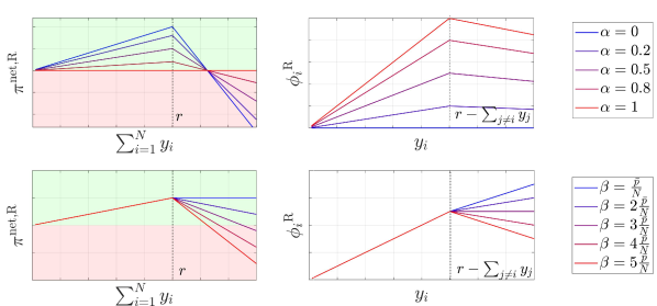
Figure 1: Qualitative behaviour of the reward functions for the DSO (left) and the followers (right) for different $\alpha$ (top) and $\beta$ (bottom). Red areas correspond to a cost, while green ones correspond to a reward.

Similarly, during rebound blocks, the DSO receives an economic incentive $\pi^{\textup{B}}(\cdot|{r}):\mathbb{R}^{T}_{\leq 0}\rightarrow\mathbb{R}^{T}$ proportional to the aggregate rebound flexibility $\sum_{i=1}^{N}{k_{i}}$ provided:

$$\pi^{\textup{B}}\left(\left.\sum_{i=1}^{N}{k_{i}}\right|{r}\right)\coloneqq\begin{dcases}0,\quad\hskip 45.52458pt\>\text{if}\>r\geq 0\\ -\tilde{p}\textstyle\sum_{i=1}^{N}{k_{i}},\quad\>\text{otherwise},\end{dcases}$$ (5)

where $\tilde{p}$ is the price provided by the TSO to the DSO for unit of rebound. From the prosumers point of view, during rebound blocks the prosumers are asked to absorb extra power from the main grid to maintain its stability. In this case, we assume that the prosumers can access the $|k_{i}|$ unit of power from the main grid at zero cost. Since they will save to purchase this additional power from the grid paying $h$, the DSO does not need to share part of the revenues with the prosumers to make them contribute to the rebound. Consequently, the reward is entirely kept by the DSO for its intermediary service. The current mathematical description of the rebound does not guarantee an increment in the amount of power taken from the grid with respect to a baseline case. Nevertheless, we notice from simulations that prosumers do take advantage of rebound blocks to absorb more energy. This is a behaviour akin to the one encountered in peak-shaving schemes [4].

II-B DSO constraints and cost function

The DSO aims solely at maximizing its revenues [2]. These derive both from selling energy and from providing flexibility to the TSO. The pricing map $h$ is assumed to be affine with respect to the total energy purchased by the prosumers, as it is shown in [4],[12] that this map induces a peak-shaving behaviour.

Assumption 1 (Affine pricing map)

For an aggregate purchased power $\sum_{i=1}^{N}p_{i}$, the pricing map $h:\mathbb{R}^{T}_{\geq 0}\rightarrow\mathbb{R}^{T}$ is

$$h\left(\sum_{i=1}^{N}p_{i}\right)=C_{1}\sum_{i=1}^{N}p_{i}+c_{0},$$ (6)

where $C_{1}=\text{diag}(c_{1})$ with $c_{1},c_{0}\in\mathbb{R}^{T}_{\geq 0}$. ∎

While $c_{0}$ is a parameter that is optimized by the DSO, $c_{1}$ is assumed to be fixed and used to model the peak price throughout the prediction horizon. This assumption prevents the presence of tri-linear terms in the cost function that would highly complicate the analysis.

A second stream of revenues for the DSO comes from the reward for the provision of DR services that is not redistributed to the agents, viz. $\mathds{1}_{T}^{\top}\pi^{\text{net,R}}\left(\left.\sum_{i=1}^{N}{y_{i}}\right|r\right)$ and $\mathds{1}_{T}^{\top}\pi^{\textup{B}}\left(\left.\sum_{i=1}^{N}{k_{i}}\right|r\right)$ . Therefore, the resulting cost function for the DSO reads as

$${J}^{\textup{DSO}}\coloneqq-\left(C_{1}\sum_{i=1}^{N}p_{i}+c_{0}\right)^{\top}\sum_{i=1}^{N}p_{i}-\mathds{1}_{T}^{\top}(\pi^{\textup{net,R}}+\pi^{\textup{B}}),$$ (7)

where we dropped the arguments of the rewards for the sake of a lighter notation.

Note that in (7) we omit the cost that the DSO has to incur to purchase power from the main grid. Alternatively, if one considers the electricity selling price $s$ from the main grid to the DSO to be proportional (or affine) to the aggregate power $\sum_{i=1}^{N}p_{i}$, then it is possible to incorporate it into the first term of (7), without changing the problem formulation.

The variables $c_{0},\alpha\in\mathbb{R}^{T}$ are subject to the following box constraints, $\underline{c_{0}}\leq c_{0}\leq\overline{c_{0}}$ and $0\leq\alpha\leq 1$. Here, the constraints on $c_{0}$ are used to prevent the DSO from raising the price coefficients unrealistically, since we are modeling a monopoly. The constraints over $\alpha$ ensure that the term is indeed a fraction.

II-C Prosumer constraints and cost function

We assume that each prosumer aims to meet its power demand at the minimum cost. Therefore, the cost function of each prosumer is the sum of four contributions

$$J^{i}\coloneqq \underbrace{\left(C_{1}\sum_{i=1}^{N}p_{i}+c_{0}\right)^{\top}p_{i}}_{\text{power purchasing cost}}-\underbrace{\vphantom{\left(C_{1}\sum_{i=1}^{N}p_{i}+c_{0}\right)^{\top}}\mathds{1}_{T}^{\top}\bigg{(}(I_{T}-\Delta)\phi_{i}^{\textup{R}}\bigg{)}}_{\text{response reward}}$$ (8)

$$+\underbrace{\vphantom{\left(C_{1}\sum_{i=1}^{N}p_{i}+c_{0}\right)^{\top}}\delta\left(p_{i}^{\textup{C}}+p_{i}^{\textup{DC}}\right)}_{\text{storage degradation cost}}+\underbrace{\vphantom{\left(C_{1}\sum_{i=1}^{N}p_{i}+c_{0}\right)^{\top}}\mu y_{i}}_{\text{discomfort cost}},$$

where $\delta>0$ is a degradation weight and $0\leq\mu<<\bar{p}$ is a (small) discomfort weight. For each time interval $\tau\in\{1,\ldots,T\}$, the $i$-th prosumer must schedule its electric storage and define the flexibility to provide when requested. The affine local set of constraints describing the dynamic evolution of the state of charge of the storage device reads as

$$e_{i,\tau}=e_{i,\tau-1}+\Delta\tau\big{(}\eta^{\textup{C}}p^{\textup{C}}_{i,\tau}-\eta^{\textup{DC}}p^{\textup{DC}}_{i,\tau}\big{)},$$ (9a)

$$0\leq p^{\textup{C}}_{i,\tau}\leq p^{\max}_{i},$$ (9b)

$$0\leq p^{\textup{DC}}_{i,\tau}\leq p^{\max}_{i},$$ (9c)

$$0\leq e_{i,\tau}\leq e^{\max}_{i},$$ (9d)

$$p_{i,\tau}-k_{i,\tau}\geq d_{i,\tau}-s_{i,\tau}+p^{\textup{C}}_{i,\tau}-p^{\textup{DC}}_{i,\tau},$$ (9e)

where $e_{i}$ is the state of charge of the electric storage device and $e_{i,0}$ its initial state, while $\eta^{C}$ and $\eta^{DC}$ are the charging and discharging efficiency of the storage device, respectively. The prosumer’s fixed load is denoted by $d_{i}$, while $s_{i}$ stands for the produced renewable power. We assume that the local demand of each prosumer is higher or equal than the local renewable power generated. Thus, we do not model sell-back programs and/or curtailment. As a consequence, $d_{i}-s_{i}+p_{i}^{\textup{C}}-p_{i}^{\textup{DC}}\geq 0$, thus $p_{i}\geq 0$.

II-D Coupling constraint

Finally, the last set of constraint couples the energy consumption of prosumers:

$$\sum_{i=1}^{N}p_{i}+\sum_{i=1}^{N}y_{i}-\sum_{i=1}^{N}k_{i}\leq\max(g,g-r)$$ (10a)

$$\sum_{i=1}^{N}|k_{i}|\leq|r|,$$ (10b)

where $g\in\mathbb{R}_{\geq 0}^{T}$ is the resource vector representing the grid capacity. Loosely speaking, in (10a) the grid capacity $g$ is artificially reduced during the DR response blocks of a quantity $\sum_{i=1}^{N}y_{i}$. On the other hand, during rebound blocks $g$ is physically enlarged. We stress the difference between response which results in a virtual restriction of the resource vector and rebound which implies a physical enlargement of it. Finally, (10b) prevents prosumers from taking more units of energy for free than the ones requested by the TSO rebound signal.

II-E Discussion of alternative design choices

Throughout Section I, we have introduced several design choices. We briefly motivate them here, comparing them with possible alternatives. Alternative market designs are:

• The DSO sells power at a discounted price during rebound blocks instead of for free. This would increase the symmetry between the response and rebound blocks.

• Some users are still allowed to absorb extra amount of power during response blocks, as long as on a global scale there is still a reduction (and viceversa for rebound blocks). This would increase the action space of the prosumers, leading to possibly lower costs.

• The DSO dynamically adjusts the coefficients in the $h$ function to encourage prosumers to offer flexibility without the need of a separate incentive scheme.

While the first two choices provide similar formulations to the proposed one in terms of theoretical properties and market operations, the third choice would lead to a different market structure where the benefits of providing flexibility are global (i.e., via the pricing map $h$) instead of proportional to the individual effort sustained by each prosumer as proposed. This might lead to unfair situations with the presence of free-riders.

III Stackelberg game

III-A Reformulation as bilevel optimization program

We are now ready to recast the DR scheme as a Stackelberg game with one leader and $N$ followers as in (1).

The affine reward functions for the response, $\pi^{\textup{R}}(\sum_{i=1}^{N}y_{i},|r)$ and $\phi^{\textup{R}}_{i}(y_{i},\boldsymbol{y}_{-i}|r)$, introduce nonlinearities. To proceed with the analysis, we implement an epigraph reformulation and replace them with auxiliary variables. As an illustrative example, let us consider the term $\min_{y_{i}}-\phi^{\textup{R}}_{i}(y_{i},\boldsymbol{y}_{-i}|r)$ in (8) for a fixed time step $\tau$. It can be shown [13, Sec. 4.1] that it is equivalent to the following epigraph reformulation

$$\begin{array}[]{l}\underset{y_{i,\tau},t_{i,\tau}}{\min}\hskip 5.69046ptt_{i,\tau}\\ \text{s.t.}\hskip 11.38092ptt_{i,\tau}\leq 0\\ \hskip 22.76228ptt_{i,\tau}\geq-\bar{p}y_{i,\tau}\\ \hskip 22.76228ptt_{i,\tau}\geq-\left((\bar{p}-\beta)y_{i,\tau}+\beta\left({r}-\textstyle\sum_{j\in\mathcal{N}\setminus\{i\}}y_{j,\tau}\right)\right),\end{array}$$ (11)

where $t_{i,\tau}\in\mathbb{R}$ is an auxiliary variable. From the point of view of the leader, this reformulation simply amounts to replacing (4) by $-(I_{N}-\Lambda)\textstyle\sum_{i=1}^{N}t_{i}$. The rebound case, on the other hand, does not present any nonlinearity in the domain where $k_{i}$ is defined, see (5). Note that the epigraph reformulation above introduces a series of additional local and coupling constraint inequalities.

Next, we define the feasible decision sets for both the leader and the followers. Starting from the DSO, the collective leader strategy $z_{0}\coloneqq\text{col}(c_{0},\alpha)$ has to satisfy box constraints (cfr. Subsection II-B); thus we can write the DSO feasible set compactly as

$${\Gamma}\coloneqq\left\{z_{0}\in\mathbb{R}_{\geq 0}^{2T}\>:\>F^{\textup{DSO}}z_{0}\leq g^{\textup{DSO}}\right\}.$$ (12)

Note that $\Gamma$ is nonempty if $\overline{c_{0}}\geq\underline{c_{0}}\geq 0$ and it is compact. The local feasible decision of the $i$-th prosumer is denoted by ${x}_{i}\coloneqq\text{col}(p_{i},y_{i},e_{i},p_{i}^{\textup{C}},p_{i}^{\textup{DC}},k_{i},t_{i})\in\mathbb{R}^{7T}$. Prosumer $i$ has to satisfy (9), (11) and the non-negativity (respectively, non-positivity) bounds on $y_{i}$ (respectively, $k_{i}$) represented in compact form as as $F_{i}x_{i}\leq f_{i}$. Therefore the local feasible decision set is $\Omega_{i}\coloneqq\left\{x_{i}\in\mathbb{R}^{7T}:F_{i}x_{i}\leq f_{i}\right\}$, where $\Omega_{i}$ is a compact set as all variables are bounded (see (9), (10) and recall the no sell-back programs assumption). Additionally, the coupling constraints in (10) can be compactly written as ${A}_{i}{x}_{i}+\sum_{j\in\mathcal{N}}{A}_{j}{x}_{j}\leq{b}$. Therefore, the followers feasible decision set becomes

$${\mathcal{X}}_{i}(\boldsymbol{x}_{-i})\coloneqq\left\{x_{i}\in\Omega_{i}:{A}_{i}{x}_{i}+\sum_{j\in\mathcal{N}\setminus\{i\}}{A}_{j}{x}_{j}\leq{b}\right\}.$$ (13)

We introduce some blanket assumptions on this set of feasible strategy, standard in the literature [9].

Assumption 2

For each player $i\in\mathcal{N}$, the set $\Omega_{i}$ is nonempty. The collective feasible set $\boldsymbol{\mathcal{X}}\coloneqq\prod_{i\in\mathcal{N}}\mathcal{X}_{i}(\boldsymbol{x}_{-i})$ satisfies Slater’s constraint qualification.

Note that, Slater’s constraint qualification can be easily met by choosing a resource vector $g$ large enough.

We reorganize the cost functions (7) and (8) in a compact matrix form as

$$J^{\textup{DSO}}({z}_{0},\boldsymbol{{x}})={f_{0}({z}_{0})}+{f_{x}(\boldsymbol{{x}})}+{\left(\sum_{i\in\mathcal{N}}f_{0,i}({x}_{i})\right)^{\top}{z}_{0}},$$ (14)

$$J^{i}\left({x}_{i},\boldsymbol{{x}}_{-i}|{z}_{0}\right)= {x}_{i}^{T}Q{x}_{i}+\left(\sum_{j\in\mathcal{N}\setminus\{i\}}Q{x}_{j}+C_{i,0}{z}_{0}\right)^{\top}{x}_{i},$$ (15)

for an appropriate choice of $f_{0}$, $f_{x}$, $f_{0,i}$, and $C_{i,0}$. For all $j,k\in\{1,\cdots,7T\}$, $Q$ is defined component wise as

$$[Q]_{jk}\coloneqq\begin{cases}1&\text{if }j=k\text{ and }j\leq T\\ 0&\text{oth.}\end{cases}.$$ (16)

At this point, we have recast the Stackelberg game between the DSO and the $N$ prosumers as a bilevel optimization problem as anticipated in (1).

III-B Stackelberg equilibrium

Next, we discuss the equilibrium concept associated to the Stackelberg game in (1). For a fixed strategy of the leader, $z_{0}$, the followers take part in a Generalized Nash Equilibrium Problem (GNEP). In general, solving a GNEP is a difficult task and does not allow for a nice formulation of the set of all solutions that can be exploited by the leader during the optimization. For this reason, we focus on the subset of v-GNE. This set of equilibria represent a “fair” competition among followers, since they equally share the cost of satisfying the coupling constraints, see [14]. The set of v-GNE can be characterized as the solution set of variational inequalities $\mathrm{VI}(\boldsymbol{\mathcal{X}},H(z_{0},\cdot))$, where $H(z_{0},\boldsymbol{x})\coloneqq\text{col}((\nabla_{x_{i}}J^{i}(z_{0},\boldsymbol{x}))_{i\in\mathcal{N}})$ is the pseudo-gradient mapping of the followers game [14]. For any given $z_{0}$, this set of v-GNE reads as,

$$\mathcal{S}(z_{0})\coloneqq\{\boldsymbol{x}\in\boldsymbol{\mathcal{X}}{\color[rgb]{0,0,1}:}(\boldsymbol{w}-\boldsymbol{x})^{\top}H(z_{0},\boldsymbol{x})\geq 0,\forall\boldsymbol{w}\in\boldsymbol{\mathcal{X}}\}.$$ (17)

Next, we show that this solution set is nonempty and compact.

Lemma 1 (Existence of v-GNE)

The set of v-GNE $\mathcal{S}(z_{0})$ in (17) is nonempty and compact for all $z_{0}\in\Gamma$.

Proof:

From [15, Th. 6] it follows that the continuity of $H(z_{0},\cdot)$ and the compactness of $\boldsymbol{\mathcal{X}}$ entails the existence of a solution to VI($H(z_{0},\cdot),\boldsymbol{\mathcal{X}}$), i.e., $\mathcal{S}(z_{0})\neq\emptyset$. Additionally [16, Th. 2.2.5] ensures the compactness of $\mathcal{S}(z_{0})$. ∎

We can rewrite the complete DR problem as

$$\left\{\begin{aligned} \min_{z_{0},\boldsymbol{x}}&\quad J^{\textup{DSO}}\left(z_{0},\boldsymbol{x}\right)\\ \text{ s.t. }&\quad\left(z_{0},\boldsymbol{x}\right)\in{\operatorname*{gph}(\mathcal{S})\cap(\Gamma\times\mathbb{R}^{n})},\end{aligned}\right.$$ (18)

that is a MPEC. This class of problems is inherently non-convex and typically hard to solve. In general, there is no guarantee that feasible solutions strictly lie in the interior of the feasible set, which may even be disconnected. As a consequence, constraint qualifications may be violated at every feasible point. For this reason we focus on seeking local solutions of (18).

We consider the following definition of local generalized Stackelberg equilibrium from [9].

Definition 1 (Local generalized Stackelberg equilibrium)

A pair $(z_{0}^{\star},\boldsymbol{x}^{\star})\in\operatorname*{gph}(\mathcal{S})\cap(\Gamma\times\mathbb{R}^{n})$, with $\mathcal{S}$ as in (17), is a $\ell$-SE of the game in (18) (and thus of (1)) if there exist open neighborhoods $\mathcal{O}_{z_{0}^{\star}}$ and $\mathcal{O}_{\boldsymbol{x}^{\star}}$ of $z_{0}^{\star}$ and $\boldsymbol{x}^{\star}$ respectively, such that

$$J^{\textup{DSO}}\left(z_{0}^{\star},\boldsymbol{x}^{\star}\right)\leq\inf_{(z_{0},\boldsymbol{x})\in\operatorname*{gph}(\mathcal{S})\cap(\Gamma\times\mathbb{R}^{n})\cap\mathcal{O}}J^{\textup{DSO}}\left(z_{0},\boldsymbol{x}\right)$$ (19)

where $\mathcal{O}\coloneqq\left(\mathcal{O}_{z_{0}^{\star}}\times\mathcal{O}_{\boldsymbol{x}^{\star}}\right)$.

Roughly speaking, at an $\ell$-SE, the DSO and the prosumers locally fulfill the set of mutually coupling constraints and none of them can achieve a lower cost by unilaterally deviating from their current strategy.

Theorem 1 (Existence of $\ell$-SE)

Under Assumption 2, there exists at least one $\ell$-SE of the MPEC in (18).

Proof:

From Lemma 1, for all $\bar{z}_{0}\in\Gamma$ there exists an $\bar{\boldsymbol{x}}$ such that $(\bar{z}_{0},\bar{\boldsymbol{x}})\in\operatorname*{gph}(\mathcal{S})$, therefore $\operatorname*{gph}(\mathcal{S})\cap(\Gamma\times\mathbb{R}^{n})\neq\emptyset$ and it is compact since it is an intersection of compact sets.

From [17, Th. 1.3.4] and the continuity of the cost function $J^{\textup{DSO}}$ with respect to $z_{0}$, we conclude the existence of a solution to the MPEC in (18), that in turns satisfies the definition in (19).

∎

III-C Solution method

To solve the VI in (18), we exploit the strong relation between v-GNEs and KKT of the followers’ game. The KKT conditions of the follower level read in a compact form as

$$\left\{\begin{array}[]{l}\boldsymbol{Q}\boldsymbol{x}+Cz_{0}+A^{\top}\lambda+F^{\top}\boldsymbol{\lambda}=0\\ 0\leq\lambda\perp-(A\boldsymbol{x}-b)\geq 0\\ {0\leq\boldsymbol{\lambda}\perp-\left(F\boldsymbol{x}-f\right)\geq 0,}\end{array}\right.$$ (20)

where $\lambda$ is the dual variable associated with the coupling constraints $A\boldsymbol{x}\leq b$. The (local) dual variable $\lambda_{i}$ is associated with the (local) constraints of each follower $i\in\mathcal{N}$ and $\boldsymbol{\lambda}\coloneqq\text{col}((\lambda_{i})_{i\in\mathcal{N}})$, while $F\coloneqq\text{diag}((F_{i})_{i\in\mathcal{N}})$, and $f\coloneqq\text{col}((f_{i})_{i\in\mathcal{N}})$. The matrices in the costs are $\boldsymbol{Q}\coloneqq(I_{N}+\mathbb{1}_{N\times N})\otimes Q$ and $C\coloneqq\left[\begin{array}[]{ccc}C_{1,0}^{\top}&\ldots&C_{N,0}^{\top}\end{array}\right]^{\top}$. The following lemma ensures that if a collective strategy satisfies the KKT conditions, then it is also a v-GNE.

Lemma 2 (KKT reformulation [17, Th. 1.3.5])

Given any $z_{0}\in\Gamma$, the strategy $\boldsymbol{x^{\star}}\in\mathcal{S}(z_{0})$ if and only if there exists a triplet $(\boldsymbol{x^{\star}},\boldsymbol{\lambda}^{\star},\lambda^{\star})$ satisfying the KKT conditions in (20).

Substituting (20) back into (18), we obtain a single-level optimization problem

$$\begin{cases}\min_{y_{0},\boldsymbol{x},\lambda,\boldsymbol{\lambda}}&J^{\textup{DSO}}\left(z_{0},\boldsymbol{x}\right)\\ \text{ s.t. }&\boldsymbol{Q}\boldsymbol{x}+Cz_{0}+A^{\top}\lambda+F^{\top}\boldsymbol{\lambda}=0\\ &0\leq{\boldsymbol{\lambda}}\perp-\left({F\boldsymbol{x}-f}\right)\geq 0,\\ &0\leq\lambda\perp-(A\boldsymbol{x}-b)\geq 0\\ &z_{0}\in\Gamma,\end{cases}$$ (21)

that can be solved with one of the methods for MPEC proposed in [18].

IV Simulations

We apply our hierarchical DR scheme to a community of residential buildings equipped with an array of photovoltaic panels and a battery for electric storage. We consider a small-scale community of $N=5$ residential buildings during the heating season. Building loads are simulated in EnergyPlus via the Cesar-p interface [19] using building characteristic input files corresponding to different prototypical Swiss residential buildings. Weather data are from MeteoSwiss, while electricity prices are from EPEX spot market. We simulate the demand response scheme throughout one day with hourly resolution, i.e., $\tau\in\{1,\ldots,24\}$, with a random flexibility request ${r}$ signal encompassing both response and rebound blocks. For small-scale instances, (21) can be solved in a centralized manner relying on a big-M reformulation with empirically tuned $M$-constants [20], returning a MIQP. In Figure 2, we report the behaviour of prosumer $1$. Results for the remaining agents are similar and omitted in the interest of space. As expected, the agents tend to charge their battery during rebound periods (see, for instance, interval $[1-3]$ h in Figure 2) and discharge it during response periods (see, for instance, interval $[3-6]$ in Figure 2). As reported in Figure 3 (top plot), the community of buildings is able to contribute to the flexibility provision task, with each building contributing proportionally to its battery size. The inability to provide the full upward flexibility request during some time steps, for instance in the interval $[8-9]$ h is due to a limited resource vector $g$ that forces the buildings to first satisfy their internal demand. On the contrary, the inability to meet the downward flexibility request (see, for instance, interval $[1-2]$ h) is a consequence of physical constraints on the size/ramping of the battery. Additionally, Figure 3 (bottom plot) suggests that the affine pricing map $h$ implicitly promotes peak shaving [4]. During rebound blocks, the overall power taken from the grid, i.e., $\sum_{i=1}^{N}p_{i}-k_{i}$, is higher than the baseline case, akin to a “valley-filling" behaviour. Finally, we report the distribution share and the pricing map $h$ decided by the DSO in Figure 4. Interestingly, a pattern seems to emerge between $\alpha$ and $h$ with electricity prices lowering considerably during response blocks. This anti-phase behaviour can be explained by considering that a competition between the DSO’s objectives might arise: while the flexibility provision objective tends to reduce the amount of power to be purchased, the first term in (7) would indeed benefit from an increase in it, thus the DSO tends to offer “reduced" prices to encourage more buying.

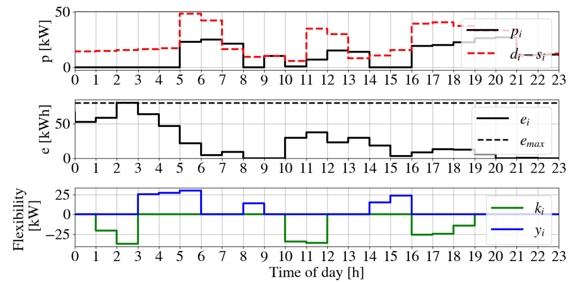
Figure 2: Behaviour of prosumer $i=1$ during the DR day-ahead scheduling.

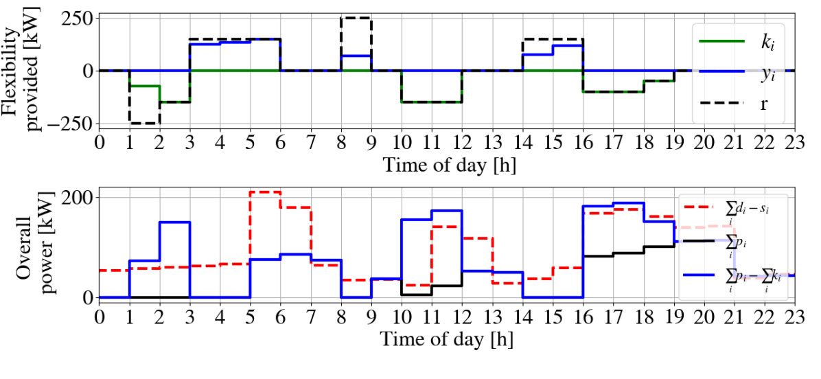
Figure 3: Top plot represents the aggregated power purchased from the grid. Bottom plot represents the aggregated flexibility provision offered by the buildings community.

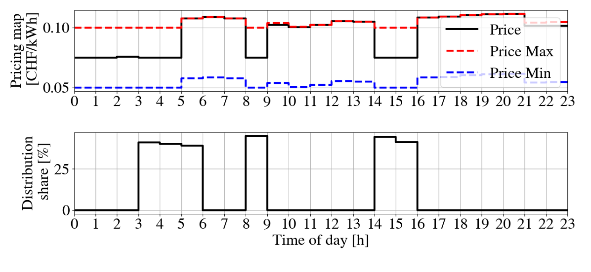
Figure 4: Top plot represents the pricing map $h$. Bottom plot represents the distribution share $\alpha$.

V Conclusion

We present a novel demand response scheme modelled as a Stackelberg game between a DSO and a community of prosumers. The scheme is able to couple the local electricity market with ancillary service provision ensuring at the same time fairness. Additionally, it allows a broader action space to both the DSO (thanks to the two different revenue streams in place) and the prosumers (thanks to the usage of saturated reward function). We prove the existence and convergence to local Stackelberg equilibria for the underlying game.

References

- [1] C. E. r. European Commission. [Online]. Available: https://cordis.europa.eu
- [2] A. Henggeler, M. J. Carlos Alves, and B. Ecer, “Bilevel optimization to deal with demand response in power grids: models, methods and challenges,” Springer, vol. 28, p. 814–842, 2020.
- [3] A. Kovacs, “Bilevel programming approach to demand response management with day-ahead tariff,” Journal of Modern Power Systems and Clean Energy, vol. 7, p. 1632–1643, 2019.
- [4] M. Zugno, J. M. Morales, P. Pinson, and H. Madsen, “A bilevel model for electricity retailers’ participation in a demand response market environment,” Energy Economics, vol. 36, pp. 182–197, 2013.
- [5] J. S. Vardakas, N. Zorba, and C. V. Verikoukis, “A survey on demand response programs in smart grids: Pricing methods and optimization algorithms,” IEEE Communications Surveys and Tutorials, vol. 17, no. 1, pp. 152–178, 2015.
- [6] S. Dempe, V. Kalashnikov, G. A., Pérez-Valdés, and N. Kalashnykova, Bilevel Programming Problems: Theory, Algorithms and Applications to Energy Networks, 2015.
- [7] N. Qi, L. Cheng, F. Liu, X. Zhou, and F. You, “Optimal Mechanism Design for Incentive-Based Demand Response Based on Stackelberg Game,” pp. 2089–2096, 2020.
- [8] K. Alshehri, J. Liu, X. Chen, and T. Başar, “A Stackelberg Game for Multi-Period Demand Response Management in the Smart Grid,” pp. 5889–5894, 2015.
- [9] F. Fabiani, M. A. Tajeddini, H. Kebriaei, and S. Grammatico, “Local Stackelberg Equilibrium Seeking in Generalized Aggregative Games,” IEEE Transactions on Automatic Control, vol. 67, no. 2, pp. 965–970, 2022.
- [10] S. Dempe, Foundations of Bilevel Programming, 2002.
- [11] C. Kok, J. Kazempour, and P. Pinson, “A DSO-Level Contract Market for Conditional Demand Response,” pp. 1–6, 2019.
- [12] C. Cenedese, F. Fabiani, M. Cucuzzella, J. M. Scherpen, M. Cao, and S. Grammatico, “Charging plug-in electric vehicles as a mixed-integer aggregative game,” in 2019 IEEE 58th Conference on Decision and Control (CDC). IEEE, 2019, pp. 4904–4909.
- [13] S. Boyd and L. Vandenberghe, Convex Optimization, 2004.
- [14] F. Facchinei and J.-S. Pang, Finite-Dimensional Variational Inequalities and Complementarity Problems. Springer Science and Business Media, 2007.
- [15] F. Facchinei and C. Kanzow, Eds., Generalized Nash Equilibrium Problems. New York NY: Springer New York, 2017.
- [16] F. Facchinei and J.-S. Pang, Eds., Methods for Monotone Problems. New York, NY: Springer New York, 2003.
- [17] Z.-Q. Luo, J.-S. Pang, and D. Ralph, Mathematical Programs with Equilibrium Constraints. Cambridge University Press, 1996.
- [18] ——, Mathematical Programs with Equilibrium Constraints. Cambridge University Press, 1996.
- [19] L. Fierz. [Online]. Available: https://doi.org/10.5281/zenodo.5148531
- [20] J. Fortuny-Amat and B. McCarl, “A Representation and Economic Interpretation of a Two-Level Programming Problem,” Journal of Operations Reserach Society, vol. 32, p. 783–792, 1981.