Particle Creation and Entanglement in Dispersive Model with Step Velocity Profile

Abstract

We investigate particle creation and entanglement structure in a dispersive model with subluminal dispersion relation. Assuming the step function spatial velocity profile of the background flow, mode functions for a massless scalar field is exactly obtained by the matching method. Power spectrums of created particles are calculated for the subsonic and the transsonic flow cases. For the transsonic case, the sonic horizon exists and created particles show the Planckian distribution for low frequency region but the thermal property disappears for high frequency region near the cutoff frequency introduced by the non-linear dispersion. For the subsonic case, although the sonic horizon does not exist, the effective group velocity horizon appears due to the non-linear dispersion for high frequency region and approximate thermal property of the power spectrum arises. Relation between particle creation and entanglement between each mode is also discussed.

I Introduction

Quantum field theory in black hole spacetimes predicts emission of thermal Hawking radiation from black holes, of which temperature is given by the surface gravity at their event horizons [1, 2] . This property of Hawking radiation from black holes suggests that black holes behave as a kind of thermodynamical objects and the theory of black hole thermodynamics is formulated [3]. Thermal property of Hawking radiation leads to a problem called the information loss paradox, and for deeper understanding of this issue, analysis of entanglement between Hawking mode (Hawking radiation) and its partner mode has been done to investigate the quantum informational aspect of the black hole evaporation [4]. Investigations of entanglement for analog models of black holes also have been done recently [5, 6, 7, 8].

The original Hawking’s scenario implies that low energy radiations are originated from high energy region above the Planckian scale, at which quantum gravitational physics will become important. Thus it is crucial to clarify effect of the Planckian scale cutoff on the thermal property of Hawking radiation (the trans-Planckian problem) [9, 10]. To resolve this problem, it is necessary to consider the origin of the particle radiated from the black hole. If we consider time reversed evolution of emission of Hawking radiation, frequencies of emitted radiations increases exponentially as they approach the black hole horizon and exceeds the Planckian frequency, beyond that frequency, quantum effect of gravity may become important. To investigate such a situation, Unruh proposed sonic analog of black holes [11, 12]; he found that the equation of sonic waves in moving fluid has the same form as a massless scalar field in curved spacetimes, of which metric has the similar structure as black hole spacetimes. The acoustic metric corresponds to the black hole spacetime with Painlevé coordinates

$$ds^{2}=-c^{2}dt^{2}+(dx-v(x)dt)^{2},\quad v(x)=-c\sqrt{x_{s}/x}$$ (1)

where $x_{s}$ is the Schwarzschild radius and $c$ is the light velocity. The cutoff wave number $k_{0}$ is introduced as the distance between atoms constituting fluid. He numerically calculated the power spectrum of the radiation for the analog black hole with the high frequency cutoff and has shown that this cutoff does not affect the spectrum of Hawking radiation in a low frequency region.

Owing to introduction of the frequency cutoff, the Lorentz invariance of the system is broken and additional wave modes associated with the cutoff appear. Owing to these modes, Hawking radiation in analog black holes is emitted by a process that the Planckian modes transformed into the low energy modes (mode conversion). If the velocity profile $v(x)$ is a slowly changing function of the spatial coordinate, a lot of analyses have been done so far based on the WKB method. These studies show that for $\omega,\kappa\ll k_{0}$ where $\kappa$ is the first derivative of the velocity profile at the sonic horizon, the temperature of the radiation is given by $\kappa/(2\pi)$ and it coincides with Hawking’s results [10, 13, 14, 16, 17].

If the velocity profile is not slowly changing function of the spatial coordinate and expected temperature of analog black holes is high, several studies of particle creations in analog models [18, 19, 15, 16, 20] show that the spectrum of the radiation is determined not only by the first derivative of the fluid velocity at the sonic horizon, but it also depends on other parameters including the frequency cutoff. Although mechanism of radiation from analog black holes with high temperature does differs from the original Hawking radiation, it is important to study entanglement of involved modes for such a case to understand effect of the frequency cutoff on emission mechanism of radiation. In this paper, we consider an analog model with a step function velocity profile of the background flow, and apply the step discontinuous method introduced by [15, 19, 16] to evaluate Bogoliubov coefficients. Then we calculate number density of created particles and entanglement negativity between involved modes. The present study may have overlaps with the analysis by X. Busch and R. Parentani [5], in which entanglement structure for high temperature analog black hole was studied. Our analysis differs from their work in several points; first, we calculated the multipartite entanglement between modes. Second, we consider two different types of analog spacetimes; the one with a sonic horizon, and the other without a sonic horizon.

The paper is organized as follows. In Section II, we shortly review particle creation in analog system with the dispersive media. In Section III, we determine the Bogoliubov coefficients for the step function velocity profile. In Section IV, we investigate entanglement structure of the in-vacuum state. In Section V, we show results of our numerical calculation. Section VI is devoted to summary and conclusion. We used the unit $c=\hbar=G=1$ throughout this paper.

II Wave modes for steep velocity profile

We consider wave modes of an analog model with dispersive media. We adopt the following wave equation of a massless real scalar field

$$(\partial_{t}+\partial_{x}v(x))(\partial_{t}+v(x)\partial_{x})\phi(x,t)=c_{s}^{2}(-i\partial_{x})\,\partial_{x}^{2}\phi(x,t).$$ (2)

This is the equation for sonic waves in a moving fluid with a position dependent velocity profile $v(x)$ and the sound velocity $c_{s}(k)$ with the wave number $k=-i\partial_{x}$. In the following, we assume that the velocity of the fluid has the step function profile

$$v(x)=V_{-}+(V_{+}-V_{-})\,\theta(x),\quad V_{\pm}<0,$$ (3)

and the flow velocity in $x>0$ region is subsonic $V_{+}>-1$. We assume subluminal dispersion $c_{s}^{2}(k)=1-k^{2}/k_{0}^{2}$ with the cutoff of wave number $k_{0}$. The sonic horizon exists at $x=0$ if $v(0)=(V_{+}+V_{-})/2<-1$ and in such a case, the region $x<0$ becomes supersonic (inside of the sonic horizon). We will see in the next subsection A, even when whole region is subsonic and there is no sonic horizon, owing to dispersive property of the fluid for high frequency, there exists an effective horizon (group velocity horizon) which has the similar property as the sonic horizon.

II.1 Mode Functions

For the wave equation Eq. (2) with the subluminal dispersion and the velocity profile Eq. (3), by assuming $\phi\propto e^{-i\omega t+ikx}~{}(x\neq 0)$, the dispersion relation is obtained as

$$\omega-kV_{\pm}=\pm|k|\sqrt{1-\left(\frac{k}{k_{0}}\right)^{2}},\quad\omega>0.\quad\text{(signs in no particular order)}$$ (4)

We denote $k^{\pm}_{i}(\omega)$ as solutions of the dispersion relation corresponding to $V_{\pm}$, where the index $i$ denotes a label to distinguish modes. Since the spacetime is static and the wave equation does not contain explicit time dependence, a plane wave with a frequency $\omega$ does not couple to other plane waves with different $\omega$. We call $\omega$ as the laboratory frequency and $\Omega:=\omega-kV_{\pm}$ as the comoving frequency. Note that the comoving frequency is not conserved and changes its value depending on $x$. Solutions of the dispersion relation and corresponding modes in our setup are shown in Fig. 1 using a dispersion diagram; the vertical axis is the comoving frequency and the horizontal axis is the wave number. The curve in the diagram represents the right hand side of the dispersion relation $\pm|k|\sqrt{1-(k/k_{0})^{2}}$, and the straight line represents the left hand side of the dispersion relation $\omega-kV_{\pm}$.

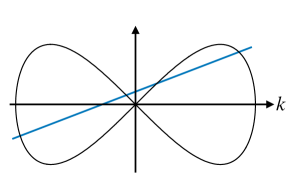
Figure 1: Dispersion diagram with the subluminal dispersion for the subsonic case. A straight line represents $\Omega=\omega-V_{\pm}\,k$. The dispersion relation has four roots which define modes. We name them as $\bar{u},v,u_{1},u_{2}$ modes in the increasing order of $k$.

From this diagram, we can identify modes as four real roots $k_{\bar{u}}$, $k_{v}$, $k_{u_{1}},k_{u_{2}}$ in the increasing order of $k$. For larger values of $\omega$ or $|V_{\pm}|$, we will have only two real solutions $k_{\bar{u}},k_{v}$ with $k<0$ and two pure imaginary solutions. One of the imaginary solutions corresponds to the decaying mode and the other imaginary solution corresponds to the growing mode. For the velocity profile with the step function (3), mode functions $\phi^{\pm}_{i}$ are plane waves

$$\phi^{\pm}_{\omega,i}(t,x)=e^{-i\omega t}\,C_{\omega,i}^{\pm}\exp\left(ik^{\pm}_{i}(\omega)x\right),\quad i=\bar{u},v,u_{1},u_{2},$$ (5)

where $C_{\omega,i}^{\pm}$ are normalization constants. We call $u_{2}^{+},\bar{u}$ as Planckian modes and $u_{1}^{+},v$ as non-Planckian modes. The Planckian modes appears due to non-linearity of the dispersion relation. On the other hand, the non-Planckian modes exist even for linear dispersion without the cutoff effect. The naming of modes depends on values of $\omega$ and $V_{\pm}$. With the increase of $\omega$, the non-Planckian mode $u_{1}$ approaches the Planckian $u_{2}$ mode. In such a situation, we call $u_{1}$ as the sub-Planckian mode. The group velocity of each mode is given by

$$v_{g}=\left(\frac{dk(\omega)}{d\omega}\right)^{-1}.$$ (6)

We present behavior of modes for the subsonic case (Fig. 2) and the transsonic case (Fig. 3). The in-modes are defined as modes with negative group velocity for $x>0$ and positive group velocity for $x<0$ (incoming to $x=0$ from $x=\pm\infty$). The out-modes are defined as modes with positive group velocity for $x>0$ and negative group velocity for $x<0$ (outgoing from $x=0$ towards $x=\pm\infty$).

For the subsonic case (Fig. 2), we assume $-1<V_{-}<V_{+}<0$. For sufficiently small $\omega$, there are four in and out modes (left panel in Fig. 2). If we increase $\omega$, the mode $u_{1}$ and the mode $u_{2}$ in $x<0$ coalesce at the critical frequency $\omega_{\text{GVH}}$, and above this frequency, we have only two out-modes in $x<0$ (right panel in Fig. 2). For $\omega_{\text{GVH}}<\omega$, $x=0$ behaves as a sonic horizon because there exists no right moving modes in $x<0$ and this region effectively becomes the supersonic region. We call this effective horizon as the group velocity horizon (GVH) [16]. There are three in-modes in $x>0$ ($u_{2},\bar{u},v$), and one out-modes in $x>0$ ($u_{1}$) and two out-modes in $x<0$ ($\bar{u},v$).

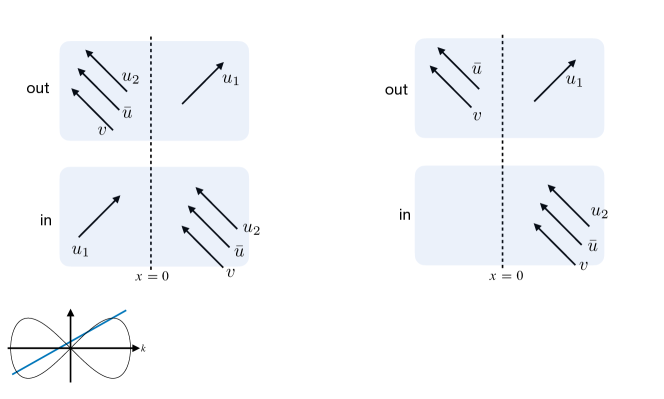
Figure 2: Dispersion diagrams and modes for the subsonic case. For $\omega<\omega_{\text{GVH}}$, the in-state and the out-state contain independent four modes. For $\omega_{\text{GVH}}<\omega$, there in no right moving modes in $x<0$ and the in-state and the out-state contain independent three modes.

For the transsonic case $V_{-}<-1<V_{+}<0$ (Fig. 3), $x=0$ is the sonic horizon. There are three in-modes in $x>0$ ($u_{2},\bar{u},v$), and two out-modes in $x<0$ ($\bar{u},v$) and one out-mode in $x>0$ ($u_{1}$). There exists no right-moving modes in the supersonic region $x<0$.

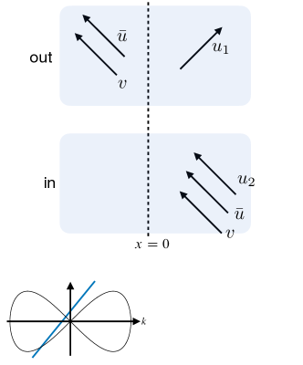
Figure 3: Dispersion diagrams and modes for the transsonic case. There is no right moving modes in $x<0$.

The incoming Planckian mode $u_{2}^{+}$ is reflected at the sonic horizon or the GVH. And it is transformed to the outgoing sub-Planckian mode $u_{1}^{+}$. This process is called the mode conversion [17]. At the same time, the Planckian mode $\bar{u}^{+}$ is transformed to the sub-Planckian mode $\bar{u}^{-}$ for the transsonic case. More detailed discussion on modes for the slowly varying velocity profile can be found in [13, 14, 16].

II.2 Quantization and vacuum state

We quantize a classical field obeying the field equation Eq. (2). The action for the field is given by

$$S=\int dt\,dx\Bigl{[}\left|(\partial_{t}+v\,\partial_{x})\phi\right|^{2}-\left|c_{s}(i\partial_{x})\,\partial_{x}\phi\right|^{2}\Bigr{]},$$ (7)

and the conjugate momentum $\pi(t,x)$ for $\phi(t,x)$ is given by

$$\pi(t,x)=(\partial_{t}+v\,\partial_{x})\phi(t,x).$$ (8)

The canonical commutation relation between quantized fields is imposed as

$$\left[\hat{\phi}(t,x),\hat{\pi}(t,y)\right]=i\,\delta(x-y).$$ (9)

The Klein-Gordon inner product on $t=\text{const.}$ surface for solutions $\phi_{1},\phi_{2}$ of the field equation is defined by

$$(\phi_{1},\phi_{2}):=-i\int dx\,\left(\phi_{1}D\phi_{2}^{*}-\phi_{2}^{*}D\phi_{1}\right)=-i\int_{\Sigma}dx~{}\left(\phi_{1}\pi_{2}^{*}-\phi_{2}^{*}\pi_{1}\right),$$ (10)

where $D=\partial_{t}+v\,\partial_{x}$ and the inner product is conserved

$$\frac{d(\phi_{1},\phi_{2})}{dt}=0.$$ (11)

With the Klein-Gordon inner product, we can define creation and annihilation operators associated with the positive norm solution $\{\phi_{i}\}$ of the wave equation by

$$\hat{a}(\phi_{i})=(\phi_{i},\hat{\phi}),\quad\hat{a}^{\dagger}(\phi_{i})=-(\phi_{i}^{*},\hat{\phi}).$$ (12)

This set of creation and annihilation operators satisfies the following commutation relations:

$$[\hat{a}(\phi_{i}),\hat{a}^{\dagger}(\phi_{j})]=(\phi_{i},\phi_{j}),\quad[\hat{a}(\phi_{i}),\hat{a}(\phi_{j})]=-(\phi_{i},\phi_{j}^{*}),\quad[\hat{a}^{\dagger}(\phi_{i}),\hat{a}^{\dagger}(\phi_{j})]=-(\phi_{i}^{*},\phi_{j}).$$ (13)

Thus if we choose a basis with ortho-normal condition, our creation and annihilation operators satisfy the standard commutation relation for the creation and annihilation operators. In general, it is not easy to construct exactly the ortho-normal basis with respect to the Klein-Gordon inner product. However, for the step function velocity profile, as all modes are represented by plane waves, it is easy to identify positive frequency modes which define a vacuum state. We note that the mode functions for $\bar{u}^{\pm}$ have negative norms and other modes have positive norms. From a vacuum state, multi-particle states are constructed by acting the creation operator on the vacuum state. We have two kinds of vacuum states. The in-vacuum state $|0_{\text{in}}\rangle$ is the state with no particle at $t\rightarrow-\infty,x\rightarrow\pm\infty$

$$\hat{a}(\phi_{i}^{\text{in}})|0_{\text{in}}\rangle=0,$$ (14)

where $\phi_{i}^{\text{in}}$ is the positive frequency mode function of the in-state for $i=u_{1}^{-},\bar{u}^{+},v^{+},u_{2}^{+}$ (sub-sonic case with $\omega<\omega_{\text{int}}$), and $i=u_{2}^{+},\bar{u}^{+},v^{+}$ (sub-sonic case with $\omega_{\text{int}}<\omega$ or trans-sonic case). The out-vacuum state $|0_{\text{out}}\rangle$ is the state with no particle at $t\rightarrow+\infty,x\rightarrow\pm\infty$,

$$\hat{a}(\phi_{i}^{\text{out}})|0_{\text{out}}\rangle=0,$$ (15)

where $\phi_{i}^{\text{out}}$ is the positive frequency mode function of the out-state for $i=\bar{u}^{-},v^{-},u_{2}^{-},u_{1}^{+}$ (sub-sonic case with $\omega<\omega_{\text{int}}$), and $i=\bar{u}^{-},v^{-},u_{1}^{+}$ (sub-sonic case with $\omega_{\text{int}}<\omega$ or trans-sonic case). In general, these two vacuum state are not equal and the number of the out-state particles in the in-state vacuum is

$$\langle 0_{\text{in}}|\hat{a}^{{\dagger}}(\phi_{i}^{\text{out}})\,\hat{a}(\phi_{i}^{\text{out}})|0_{\text{in}}\rangle\neq 0.$$ (16)

This implies particle creation occurs at $x=0$.

The filed operator is expanded as

$$\hat{\phi}(t,x)=\sum_{i}\left(\hat{a}(\phi_{i}^{\text{in}})\phi_{i}^{\text{in}}+\text{(h.c.)}\right)=\sum_{i}\left(\hat{a}(\phi_{i}^{\text{out}})\phi_{i}^{\text{out}}+\text{(h.c.)}\right),$$ (17)

and creation and annihilation operators are represented as

$$\hat{a}(\phi_{i}^{\text{in,out}})=(\phi_{i}^{\text{in,out}},\hat{\phi}),\quad\hat{a}^{\dagger}(\phi_{i}^{\text{in,out}})=-(\phi_{i}^{\text{in,out}}{}^{*},\hat{\phi}).$$ (18)

III Bogoliubov coefficients

We can analytically determine a relation between the in-mode state and the out-mode state for the wave equation with the step function velocity profile.

III.1 Matching method

By separating time dependence of the wave function as $\propto e^{-i\omega t}$ in Eq. (2), the wave equation becomes the following ordinary differential equation

$$(-i\omega+\partial_{x}v(x))(-i\omega+v(x)\,\partial_{x})\phi(x)=\left(1+\frac{1}{k_{0}^{2}}\partial_{x}^{2}\right)\partial_{x}^{2}\,\phi(x)$$ (19)

with the velocity profile given by Eq. (3). For $x\neq 0$, the solution of this equation is superposition of plane waves $\exp(ik_{i}^{+}x)$ for $x>0$ and $\exp(ik_{i}^{-}x)$ for $x<0$. Coefficients of superposition are determined by matching conditions at $x=0$. Let us denote $\phi_{\pm}$ as the solution of Eq. (19) for $x\gtrless 0$. We impose matching conditions between $\phi_{+}$ and $\phi_{-}$ at $x=0$ as follows. We require continuity condition of $\phi$ at $x=0$ up to the second spatial derivative to ensure the well-behaved wave function. Additional condition is obtained by integrating both sides of the wave equation in the range $-\varepsilon<x<\varepsilon$, and taking $\varepsilon\to 0$:

$$-i\omega(V_{+}-V_{-})\phi(0)+(V_{+}^{2}-V_{-}^{2})\,\partial_{x}\phi(0)=\frac{1}{k_{0}^{2}}\left[\partial^{3}_{x}\,\phi^{+}(0)-\partial^{3}_{x}\,\phi^{-}(0)\right].$$ (20)

After all, we require the following four matching conditions

$$\phi^{+}(0)=\phi^{-}(0),\quad\partial_{x}\phi^{+}(0)=\partial_{x}\phi^{-}(0),\quad\partial^{2}_{x}\phi^{+}(0)=\partial^{2}_{x}\phi^{-}(0),$$

$$\partial^{3}_{x}\phi^{+}(0)=\partial^{3}_{x}\phi^{-}(0)-{k_{0}^{2}}(V_{+}-V_{-})\left\{i\omega\phi(0)-(V_{+}+V_{-})\partial_{x}\phi(0)\right\}.$$ (21)

Then the wave function $\phi(x)=\phi_{+}(x)\theta(x)+\phi_{-}(x)\theta(-x)$ is the global solution of the wave equation (19).

III.2 Bogoliubov coefficients

By using the matching formula Eq. (21), we can construct $\phi^{+}_{i}(x)$ defined for $x>0$ connected to the plane wave $e^{ik_{i}^{-}x}$ for $x<0$. $\phi^{+}_{i}(x)$ can be expressed as

$$\phi^{+}_{i}(x)=\sum_{j=1}^{4}\alpha_{ij}\exp(ik^{+}_{j}x)$$ (22)

with superposition coefficients $\{\alpha_{ij}\}$. Wave numbers $\{k^{+}_{j}(\omega)\}$ are determined by Eq. (4). The matching formula Eq. (21) yields the following equations for $\{\alpha_{ij}\}$:

$$\sum_{j}\alpha_{ij}=1,\quad\sum_{j}\alpha_{ij}\,k^{+}_{j}=k^{-}_{i},\quad\sum_{j}\alpha_{ij}\left(k^{+}_{j}\right)^{2}=\left(k^{-}_{i}\right)^{2},$$ (23)

$$\sum_{j}\alpha_{ij}\left(k^{+}_{j}\right)^{3}=\left(k^{-}_{i}\right)^{3}+{k_{0}^{2}}\,(V_{+}-V_{-})\left\{\omega-(V_{+}+V_{-})\,k^{-}_{i}\right\}.$$ (24)

By solving these relation for $\alpha_{il}$, we obtain

$$\begin{pmatrix}\alpha_{i1}\\ \alpha_{i2}\\ \alpha_{i3}\\ \alpha_{i4}\end{pmatrix}=\begin{pmatrix}-{B_{1}}/{A_{1}}&{C_{1}}/{A_{1}}&-{D_{1}}/{A_{1}}&{1}/{A_{1}}\\ -{B_{2}}/{A_{2}}&{C_{2}}/{A_{2}}&-{D_{2}}/{A_{2}}&{1}/{A_{2}}\\ -{B_{3}}/{A_{3}}&{C_{3}}/{A_{3}}&-{D_{3}}/{A_{3}}&{1}/{A_{3}}\\ -{B_{4}}/{A_{4}}&{C_{4}}/{A_{4}}&-{D_{4}}/{A_{4}}&{1}/{A_{4}}\end{pmatrix}\begin{pmatrix}1\\ k^{-}_{i}\\ (k^{-}_{i})^{2}\\ (k^{-}_{i})^{3}+{k_{0}^{2}}\,(V_{+}-V_{-})\left\{\omega-(V_{+}+V_{-})k^{-}_{i}\right\}\end{pmatrix}$$ (25)

with

$$A_{i}=(k^{+}_{i}-k^{+}_{j})(k^{+}_{i}-k^{+}_{k})(k^{+}_{i}-k^{+}_{l}),\quad B_{i}=k^{+}_{j}\,k^{+}_{k}\,k^{+}_{l},$$ (26)

$$C_{i}=k^{+}_{j}\,k^{+}_{k}+k^{+}_{k}\,k^{+}_{l}+k^{+}_{l}\,k^{+}_{j},\quad D_{i}=k^{+}_{j}+k^{+}_{k}+k^{+}_{l}.$$ (27)

$$(\text{indices }i,j,k,l\text{ are different each other}).$$

By specifying a mode in $x<0$, it is possible to obtain a wave function which satisfies a given boundary condition in $x<0$. Schematic diagrams describing possible four different boundary conditions in $x<0$ region are shown in Fig. 4.

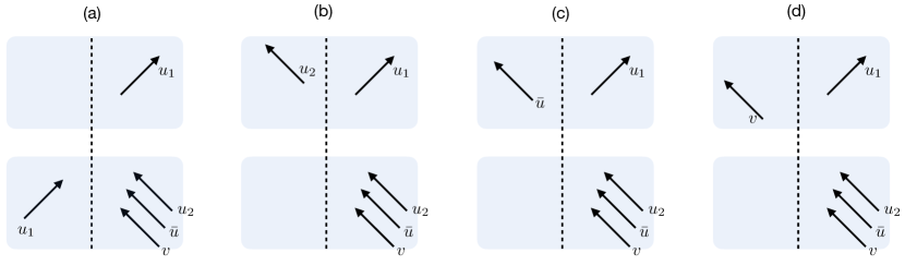
Figure 4: Four different boundary conditions in $x<0$ for the wave equation (19) to determine the Bogoliubov coefficients. (a) Boundary condition with $\phi^{-}(x)=\phi_{u_{1}}^{\text{in}}$. For the subsonic case with $\omega_{\text{GVH}}<\omega$ or the transsonic case, the mode $u_{1}$ becomes decaying mode. (b) Boundary condition with $\phi^{-}(x)=\phi_{u_{2}}^{\text{out}}$. (c) Boundary condition with $\phi^{-}(x)=\phi_{\bar{u}}^{\text{out}}$. (d) Boundary condition with $\phi^{-}(x)=\phi_{v}^{\text{out}}$.

For the plane wave $\exp(ik_{i}^{-}x)$ in $x<0$ with a real wave number $k_{i}^{-}$, we can define the normalized mode function $\phi^{\text{in/out}}_{i}(x)=\exp(i\,k_{i}^{\text{in/out}}\,x)/N^{\pm}_{i}$ with

$$N^{\pm}_{i}=\sqrt{4\pi c_{s}(k_{i}^{\pm})\,k_{i}^{\pm}\,v_{g}(k_{i}^{\pm})},\quad v_{g}=\left(\frac{dk}{d\omega}\right)^{-1}.$$ (28)

We put labels “$\pm$” and “in/out” depending on asymptotic regions and the sign of the group velocity. If all modes are normalizable (i.e. all solutions of the dispersion relation are real), plane wave solutions with specified boundary conditions are given as follows:

$$(\text{a})\quad\phi(x)=\begin{cases}N^{-}_{u_{1}}\,\phi^{\text{in}}_{u_{1}}&(x<0)\\ N^{+}_{u_{1}}\,\alpha_{u_{1}u_{1}}\,\phi^{\text{out}}_{u_{1}}+N^{+}_{u_{2}}\,\alpha_{u_{1}u_{2}}\,\phi^{\text{in}}_{u_{2}}+N^{+}_{\bar{u}}\,\alpha_{u_{1}\bar{u}}\,\phi^{\text{in}}_{\bar{u}}+N^{+}_{v}\,\alpha_{u_{1}v}\,\phi^{\text{in}}_{v}&(x>0)\end{cases}$$ (29)

$$(\text{b})\quad\phi(x)=\begin{cases}N^{-}_{u_{2}}\,\phi^{\text{out}}_{u_{2}}&(x<0)\\ N^{+}_{u_{1}}\,\alpha_{u_{2}u_{1}}\,\phi^{\text{out}}_{u_{1}}+N^{+}_{u_{2}}\,\alpha_{u_{2}u_{2}}\,\phi^{\text{in}}_{u_{2}}+N^{+}_{\bar{u}}\,\alpha_{u_{2}\bar{u}}\,\phi^{\text{in}}_{\bar{u}}+N^{+}_{v}\,\alpha_{u_{2}v}\,\phi^{\text{in}}_{v}&(x>0)\\ \end{cases}$$ (30)

$$(\text{c})\quad\phi(x)=\begin{cases}N^{-}_{\bar{u}}\,\phi^{\text{out}}_{\bar{u}}&(x<0)\\ N^{+}_{u_{1}}\,\alpha_{\bar{u}u_{1}}\,\phi^{\text{out}}_{u_{1}}+N^{+}_{u_{2}}\,\alpha_{\bar{u}u_{2}}\,\phi^{\text{in}}_{u_{2}}+N^{+}_{\bar{u}}\,\alpha_{\bar{u}\bar{u}}\,\phi^{\text{in}}_{\bar{u}}+N^{+}_{v}\,\alpha_{u_{1}v}\,\phi^{\text{in}}_{v}&(x>0)\\ \end{cases}$$ (31)

$$(\text{d})\quad\phi(x)=\begin{cases}N^{-}_{u_{1}}\,\phi^{\text{out}}_{u_{1}}&(x<0)\\ N^{+}_{u_{1}}\,\alpha_{vu_{1}}\,\phi^{\text{out}}_{u_{1}}+N^{+}_{u_{2}}\,\alpha_{vu_{2}}\,\phi^{\text{in}}_{u_{2}}+N^{+}_{\bar{u}}\,\alpha_{v\bar{u}}\,\phi^{\text{in}}_{\bar{u}}+N^{+}_{v}\,\alpha_{vv}\,\phi^{\text{in}}_{v}&(x>0)\\ \end{cases}.$$ (32)

Even if there exists unnormalizable modes, the logic is essentially same, but we have to treat the norm of modes more carefully. From Eqs. (29)-(32), we can read off relations between the in-mode functions and the out-mode functions. For example, let us consider Eq. (29). In the asymptotic out region, the wave function is expressed as $\phi(x)=N^{+}_{u_{1}}\alpha_{u_{1}u_{1}}\phi^{\text{out}}_{u_{1}}$, thus this mode defines the out-vacuum state. In the asymptotic in region, the wave function is expressed as superposition of plane waves

$$\phi(x)=N^{-}_{u_{1}}\,\phi^{\text{in}}_{u_{1}}+N^{+}_{u_{2}}\,\alpha_{u_{1}u_{2}}\,\phi^{\text{in}}_{u_{2}}+N^{+}_{\bar{u}}\,\alpha_{u_{1}\bar{u}}\,\phi^{\text{in}}_{\bar{u}}+N^{+}_{v}\,\alpha_{u_{1}v}\,\phi^{\text{in}}_{v}.$$ (33)

Therefore, we obtain the following in-out relation

$$N^{+}_{u_{1}}\,\alpha_{u_{1}u_{1}}\,\phi^{\text{out}}_{u_{1}}=N^{-}_{u_{1}}\,\phi^{\text{in}}_{u_{1}}+N^{+}_{u_{2}}\,\alpha_{u_{1}u_{2}}\,\phi^{\text{in}}_{u_{2}}+N^{+}_{\bar{u}}\,\alpha_{u_{1}\bar{u}}\,\phi^{\text{in}}_{\bar{u}}+N^{+}_{v}\,\alpha_{u_{1}v}\,\phi^{\text{in}}_{v}.$$ (34)

Repeating the same procedure for other three boundary conditions, we obtain other three in-out relations:

$$N_{u_{2}}^{-}\,\phi_{u_{2}}^{\text{out}}+N_{u_{1}}^{+}\,\alpha_{u_{2}u_{2}}\,\phi_{u_{1}}^{\text{out}}=N_{u_{2}}^{+}\,\alpha_{u_{2}u_{2}}\,\phi_{u_{2}}^{\text{in}}+N_{\bar{u}}^{+}\,\alpha_{u_{2}\bar{u}}\,\phi_{\bar{u}}^{\text{in}}+N_{v}^{+}\,\alpha_{u_{2}v}\,\phi_{v}^{\text{in}},$$ (35)

$$N_{\bar{u}}^{-}\,\phi_{\bar{u}}^{\text{out}}+N_{u_{1}}^{+}\,\alpha_{\bar{u}u_{1}}\,\phi_{u_{1}}^{\text{out}}=N_{u_{2}}^{+}\,\alpha_{\bar{u}u_{2}}\,\phi_{u_{2}}^{\text{in}}+N_{\bar{u}}^{+}\,\alpha_{\bar{u}\bar{u}}\,\phi_{\bar{u}}^{\text{in}}+N_{v}^{+}\,\alpha_{u_{1}v}\,\phi_{v}^{\text{in}},$$ (36)

$$N_{u_{1}}^{-}\,\phi_{u_{1}}^{\text{out}}+N_{u_{1}}^{+}\,\alpha_{vu_{1}}\,\phi_{u_{1}}^{\text{out}}=N_{u_{2}}\,\alpha_{vu_{2}}\,\phi_{u_{2}}^{\text{in}}+N_{\bar{u}}^{+}\,\alpha_{v\bar{u}}\,\phi_{\bar{u}}^{\text{in}}+N_{v}^{+}\,\alpha_{vv}\,\phi_{v}^{\text{in}}.$$ (37)

By taking the Klein-Gordon inner product with the field operator $\hat{\phi}$ both sides, from Eq. (18), we obtain the transformation between the in-mode operators and the out-mode operators. This transformation is the Bogoliubov transformation, and the transformation is determined by $4\times 4$ Bogoliubov coefficients. We obtain the following form of Bogoliubov transformation

$$\begin{pmatrix}-\left(\hat{a}_{\bar{u}}^{\text{out}}\right)^{\dagger}\\ \hat{a}_{v}^{\text{out}}\\ \hat{a}_{u_{1}}^{\text{out}}\\ \hat{a}_{u_{2}}^{\text{out}}\end{pmatrix}=\begin{pmatrix}\tilde{\beta}_{\bar{u}\bar{u}}&\tilde{\beta}_{\bar{u}v}&\tilde{\beta}_{\bar{u}u_{1}}&\tilde{\beta}_{\bar{u}u_{2}}\\ \tilde{\beta}_{v\bar{u}}&\tilde{\beta}_{uv}&\tilde{\beta}_{vu_{1}}&\tilde{\beta}_{vu_{2}}\\ \tilde{\beta}_{u_{1}\bar{u}}&\tilde{\beta}_{u,v}&\tilde{\beta}_{u,u_{1}}&\tilde{\beta}_{u_{1}u_{2}}\\ \tilde{\beta}_{u_{2}\bar{u}}&\tilde{\beta}_{u_{2}v}&\tilde{\beta}_{u_{2}u_{1}}&\tilde{\beta}_{u_{2}u_{2}}\end{pmatrix}\begin{pmatrix}-\left(\hat{a}_{\bar{u}}^{\text{in}}\right)^{\dagger}\\ \hat{a}_{v}^{\text{in}}\\ \hat{a}_{u_{1}}^{\text{in}}\\ \hat{a}_{u_{2}}^{\text{in}}\end{pmatrix},$$ (38)

where coefficients are given by

$$\widetilde{\beta}_{u_{1}i}=\begin{cases}\dfrac{N_{i}^{+}\,\alpha_{u_{1}i}}{N_{u_{1}}^{+}\,\alpha_{u_{1}u_{1}}}&\quad\left(i\neq u_{1}\right)\\ \dfrac{N^{-}_{u_{1}}}{N_{u_{1}}^{+}\,\alpha_{u_{1}u_{1}}}&\quad\left(i=u_{1}\right)\end{cases}$$ (39)

and

$$\widetilde{\beta}_{ij}=\begin{cases}\dfrac{N_{j}^{+}\,\alpha_{ij}-N_{u_{1}}^{+}\,\alpha_{iu_{1}}\,\tilde{\beta}_{u_{1}j}}{N_{i}^{-}}&\quad\left(j\neq u_{1}\right)\\[10.0pt] -\dfrac{N_{u_{1}}^{+}\,\alpha_{iu_{1}}\,\tilde{\beta}_{u_{1}u_{1}}}{N_{i}}&\quad\left(j=u_{1}\right)\end{cases}.$$ (40)

We obtain the Bogoliubov transformation which transforms the out-mode operators to the in-mode operators:

$$\begin{pmatrix}\left(\hat{a}_{\bar{u}}^{\text{in}}\right)^{\dagger}\\ \hat{a}_{v}^{\text{in}}\\ \hat{a}_{u_{1}}^{\text{in}}\\ \hat{a}_{u_{2}}^{\text{in}}\end{pmatrix}=\begin{pmatrix}\beta_{\bar{u}\bar{u}}&\beta_{\bar{u}v}&\beta_{\bar{u}u_{1}}&\beta_{\bar{u}u_{2}}\\ \beta_{v\bar{u}}&\beta_{uv}&\beta_{vu_{1}}&\beta_{vu_{2}}\\ \beta_{u_{1}\bar{u}}&\beta_{u_{1}v}&\beta_{u_{1}u_{1}}&\beta_{u_{1}u_{2}}\\ \beta_{u_{2}\bar{u}}&\beta_{u_{2}v}&\beta_{u_{2}u_{1}}&\beta_{u_{2}u_{2}}\end{pmatrix}\begin{pmatrix}\left(\hat{a}_{\bar{u}}^{\text{out}}\right)^{\dagger}\\ \hat{a}_{v}^{\text{out}}\\ \hat{a}_{u_{1}}^{\text{out}}\\ \hat{a}_{u_{2}}^{\text{out}}\end{pmatrix}.$$ (41)

where $\beta_{ij}$ satisfies the relation $\sum_{k}\tilde{\beta}_{ik}\beta_{kj}=\delta_{ij}$.

IV Vacuum state and covariance matrix

The Bogoliubov transformation related to the $\bar{u}$-mode is given by

$$\hat{a}_{\bar{u}}^{\text{in}}=\beta^{*}_{\bar{u}\bar{u}}\,\hat{a}_{\bar{u}}^{\text{out}}+\beta^{*}_{\bar{u}v}(\hat{a}_{v}^{\text{out}})^{\dagger}+\beta^{*}_{\bar{u}u_{1}}(\hat{a}_{u_{1}}^{\text{out}})^{\dagger}+\beta^{*}_{\bar{u}u_{2}}(\hat{a}_{u_{2}}^{\text{out}})^{\dagger},$$ (42)

where $|\beta_{\bar{u}\bar{u}}|^{2}-|\beta_{\bar{u}v}|^{2}-|\beta_{\bar{u}u_{1}}|^{2}-|\beta_{\bar{u}u_{2}}|^{2}=1$ holds. The equality $\beta_{\bar{u}u_{2}}=0$ holds for the subsonic case with the GVH and the transsonic case because there exist no $u_{2}$-mode in the out-state. The Bogoliubov coefficients related to $\bar{u}$-mode can be parameterized as

$$\beta_{\bar{u}\bar{u}}=e^{i\phi_{1}}\cosh r,\quad\beta_{\bar{u}v}=e^{i\phi_{2}}\sinh r\sin\theta,$$

$$\beta_{\bar{u}u_{1}}=e^{i\phi_{3}}\sinh r\cos\theta\sin\phi,\quad\beta_{\bar{u}u_{2}}=e^{i\phi_{4}}\sinh r\cos\theta\cos\phi,$$ (43)

where $r,\theta,\phi,\phi_{1},\phi_{2},\phi_{3},\phi_{4}$ are real parameters. $r$ is the squeezing parameter and as $r\to 0$, the number of created particles decreases. $\theta$ represents ratio of the $u$-mode and the $v$-mode; as $\theta\to 0$, mixing of $u$-mode and $v$-mode becomes small. The parameter $\phi$ represents ratio of $u_{1}$-mode and $u_{2}$-mode.

With these parameters, we can characterize the out-vacuum state. Let us define new annihilation operators ${\hat{A}_{1},\hat{A}_{2},\hat{A}_{3},\hat{A}_{4}}$ from the in-mode annihilation operators by

$$\hat{A}_{1} =\hat{a}^{\text{out}}_{\bar{u}},$$ (44)

$$\hat{A}_{2} =e^{i(\phi_{3}-\phi_{1})}\sin\theta\cos\phi\ \hat{a}^{\text{out}}_{u_{1}}+e^{i(\phi_{4}-\phi_{1})}\sin\theta\sin\phi\ \hat{a}^{\text{out}}_{u_{2}}+e^{i(\phi_{2}-\phi_{1})}\cos\theta\ \hat{a}^{\text{out}}_{v},$$ (45)

$$\hat{A}_{3} =-e^{i(\phi_{3}-\phi_{1})}\cos\theta\cos\phi\ \hat{a}^{\text{out}}_{u_{1}}-e^{i(\phi_{4}-\phi_{1})}\cos\theta\sin\phi\ \hat{a}^{\text{out}}_{u_{2}}+e^{i(\phi_{2}-\phi_{1})}\sin\theta\ \hat{a}^{\text{out}}_{v},$$ (46)

$$\hat{A}_{4} =-e^{i(\phi_{3}-\phi_{1})}\sin\phi\ \hat{a}^{\text{out}}_{u_{1}}+e^{i(\phi_{4}-\phi_{1})}\cos\phi\ \hat{a}^{\text{out}}_{u_{2}}.$$ (47)

These new operators satisfy $[\hat{A}_{i},\hat{A}_{j}]=0$ and $[\hat{A}_{i},\hat{A}_{j}^{\dagger}]=\delta_{ij}$. With these new operators, from Eq. (41), annihilation operators of the in-mode can be written as

$$\hat{a}^{\text{in}}_{\bar{u}}=e^{i\phi_{1}}(\cosh r\,\hat{A}_{1}+\sinh r\,\hat{A}_{2}^{\dagger}),$$ (48)

$$\hat{a}^{\text{in}}_{v}=e^{i\phi_{1}^{\prime}}\left[\frac{\rho}{\cosh r}(\sinh r\,\hat{A}_{1}^{\dagger}+\cosh r\,\hat{A}_{2})+\sqrt{1-\frac{|\rho|^{2}}{\cosh^{2}r}}\,(\cos\phi^{\prime}\,\hat{A}_{3}+\sin\phi^{\prime}\,\hat{A}_{4})\right],$$ (49)

$$\hat{a}^{\text{in}}_{u_{1}}=e^{i\phi_{2}^{\prime}}\left[\frac{\rho^{\prime}}{\cosh r}(\sinh r\,\hat{A}_{1}^{\dagger}+\cosh r\,\hat{A}_{2})+\sqrt{1-\frac{|\rho^{\prime}|^{2}}{\cosh^{2}r}}\,(\cos\phi^{\prime\prime}\,\hat{A}_{3}+\sin\phi^{\prime\prime}\,\hat{A}_{4})\right],$$ (50)

$$\hat{a}^{\text{in}}_{u_{2}}=e^{i\phi_{3}^{\prime}}\left[\frac{\rho^{\prime\prime}}{\cosh r}(\sinh r\,\hat{A}_{1}^{\dagger}+\cosh r\,\hat{A}_{2})+\sqrt{1-\frac{|\rho^{\prime\prime}|^{2}}{\cosh^{2}r}}\,(\cos\phi^{\prime\prime\prime}\,\hat{A}_{3}+\sin\phi^{\prime\prime\prime}\,\hat{A}_{4})\right],$$ (51)

where we introduced new constants $\phi^{\prime}_{1},\phi^{\prime}_{2},\phi^{\prime}_{3},\phi^{\prime\prime},\phi^{\prime\prime\prime},\rho,\rho^{\prime},\rho^{\prime\prime}$ which are related to original parameters $\phi_{1},\phi_{2},\phi_{3},\phi_{4},\beta_{ij}$. From these relations, the vacuum condition for the in-state yields

$$(\cosh r\,\hat{A}_{1}+\sinh r\,\hat{A}_{2}^{\dagger})\ket{0_{\text{in}}}=0,\quad(\sinh r\,\hat{A}_{1}^{\dagger}+\cosh r\,\hat{A}_{2})\ket{0_{\text{in}}}=0,$$ (52)

$$\hat{A}_{3}\ket{0_{\text{in}}}=0,\quad\hat{A}_{4}\ket{0_{\text{in}}}=0,$$ (53)

and the in-vacuum state is written as

$$|0_{\text{in}}\rangle=\frac{1}{\cosh r}\sum_{n=0}^{\infty}(-\tanh r)^{n}|n_{A_{1}}\rangle|n_{A_{2}}\rangle|0_{A_{3}}\rangle|0_{A_{4}}\rangle.$$ (54)

Thus the in-vacuum state is the two mode squeezed state of $A_{1}$-mode and $A_{2}$-mode.

To quantify entanglement between each mode using the negativity, we introduce canonical variables ${\hat{X}_{i},\hat{P}_{i}}$ by

$$\hat{X}_{i}=\frac{\hat{a}_{i}^{\text{in}}+(\hat{a}_{i}^{\text{in}})^{\dagger}}{\sqrt{2}},\quad\hat{P}_{i}=\frac{\hat{a}_{i}^{\text{in}}-(\hat{a}_{i}^{\text{in}})^{\dagger}}{i\sqrt{2}},\quad[\hat{X}_{i},\hat{P}_{j}]=i\,\delta_{ij}.$$ (55)

Then the wave function of the in-vacuum state is given as

$$\psi_{0}(X_{1},X_{2},X_{3},X_{4}) =\langle X_{1},X_{2},X_{3},X_{4}|0_{\text{in}}\rangle$$

$$=\frac{1}{\pi}\exp\left(-\frac{X_{1}^{2}+X_{2}^{2}+X_{3}^{2}+X_{4}^{2}}{2}\right).$$ (56)

The Wigner function of this wave function is defined by

$$W(\bm{X},\bm{P}) :=\frac{1}{(2\pi)^{4}}\int d^{4}\bm{Y}~{}e^{i\bm{P}\cdot\bm{Y}}\psi_{0}\left(\bm{X}-\frac{\bm{Y}}{2}\right)\psi_{0}^{*}\left(\bm{X}+\frac{\bm{Y}}{2}\right)$$

$$=\frac{1}{\pi^{3}}\exp(-\bm{X}^{2}-\bm{P}^{2}).$$ (57)

Introducing a vector with canonical variables $\hat{\bm{\xi}}=(\hat{X}_{1},\hat{P}_{1},\hat{X}_{2},\hat{P}_{2},\hat{X}_{3},\hat{P}_{3},\hat{X}_{4},\hat{P}_{4})^{T}$, the covariance matrix is defined by

$$V_{ij}:=\left\langle\frac{\hat{\xi}_{i}\,\hat{\xi}_{j}+\hat{\xi}_{j}\,\hat{\xi}_{i}}{2}\right\rangle=\int d^{8}\bm{\xi}~{}\xi_{i}\,\xi_{j}\,W(\bm{\xi}),$$ (58)

and for the wave function Eq. (56), $V_{ij}=\delta_{ij}/2$. Since the Bogoliubov transformation preserves commutation relations of creation and annihilation operators, it also keeps commutation relations between canonical variables defined in terms of creation and annihilation operators.

Now we introduce canonical variables for the out-modes as

$$\hat{x}_{i}=\frac{\hat{a}_{i}^{\text{out}}+(\hat{a}_{i}^{\text{out}})^{\dagger}}{\sqrt{2}},\quad\hat{p}_{i}=\frac{\hat{a}_{i}^{\text{out}}-(\hat{a}_{i}^{\text{out}})^{\dagger}}{i\sqrt{2}},$$

and introduce a vector with canonical variables for the in-mode as $\hat{\bm{\xi}}^{\prime}=(\hat{x}_{1},\hat{p}_{1},\hat{x}_{2},\hat{p}_{2},\hat{x}_{3},\hat{p}_{3},\hat{x}_{4},\hat{p}_{4})^{T}$. The relation between in and out canonical variables is given by

$$\hat{\xi}_{i}=\sum_{j}S_{i}^{~{}j}\,\hat{\xi}^{\prime}_{j}$$ (59)

where

$$S=\begin{pmatrix}~{}\real[\beta_{11}]&~{}\imaginary[\beta_{11}]&~{}\real[\beta_{12}]&-\imaginary[\beta_{12}]&~{}\real[\beta_{13}]&-\imaginary[\beta_{13}]&~{}\real[\beta_{14}]&-\imaginary[\beta_{14}]\\ ~{}\imaginary[\beta_{11}]&~{}\real[\beta_{11}]&~{}\imaginary[\beta_{12}]&-\real[\beta_{12}]&~{}\imaginary[\beta_{13}]&-\real[\beta_{13}]&\imaginary[\beta_{14}]&-\real[\beta_{14}]\\ ~{}\real[\beta_{21}]&~{}\imaginary[\beta_{21}]&~{}\real[\beta_{22}]&-\imaginary[\beta_{22}]&~{}\real[\beta_{23}]&-\imaginary[\beta_{23}]&~{}\real[\beta_{24}]&-\imaginary[\beta_{24}]\\ ~{}\imaginary[\beta_{21}]&~{}\real[\beta_{21}]&~{}\imaginary[\beta_{22}]&~{}\real[\beta_{22}]&~{}\imaginary[\beta_{23}]&~{}\real[\beta_{23}]&~{}\imaginary[\beta_{24}]&~{}\real[\beta_{24}]\\ ~{}\real[\beta_{31}]&~{}\imaginary[\beta_{31}]&~{}\real[\beta_{32}]&-\imaginary[\beta_{32}]&~{}\real[\beta_{33}]&-\imaginary[\beta_{33}]&~{}\real[\beta_{34}]&-\imaginary[\beta_{34}]\\ ~{}\imaginary[\beta_{31}]&-\real[\beta_{31}]&~{}\imaginary[\beta_{32}]&~{}\real[\beta_{32}]&~{}\imaginary[\beta_{33}]&~{}\real[\beta_{33}]&~{}\imaginary[\beta_{34}]&~{}\real[\beta_{34}]\\ ~{}\real[\beta_{41}]&~{}\imaginary[\beta_{41}]&~{}\real[\beta_{42}]&-\imaginary[\beta_{42}]&~{}\real[\beta_{43}]&-\imaginary[\beta_{43}]&~{}\real[\beta_{44}]&-\imaginary[\beta_{44}]\\ ~{}\imaginary[\beta_{41}]&-\real[\beta_{41}]&~{}\imaginary[\beta_{42}]&~{}\real[\beta_{42}]&~{}\imaginary[\beta_{43}]&~{}\real[\beta_{43}]&~{}\imaginary[\beta_{44}]&~{}\real[\beta_{44}]\end{pmatrix}$$ (60)

with the subscript of $\beta_{ij}$ represents $1,2,3,4=\bar{u},v,u_{1},u_{2}$. Since this transformation keeps canonical commutation relations, the matrix $S$ satisfies

$$S\,\Omega\,S^{T}=\Omega,\quad\Omega=\bigoplus_{i=1}^{4}\begin{pmatrix}0&1\\ -1&0\\ \end{pmatrix}.$$

From $|\det S|=1$, the relation between the in-mode covariance matrix $V$ and the out-mode covariance matrix $V^{\prime}$ is derived as

$$V_{ij} =\int d^{8}\bm{\xi}~{}\xi_{i}\xi_{j}\,W(\xi)=\sum_{k,l}\int d^{8}\bm{\xi}^{\prime}\,S_{i}^{~{}k}S_{j}^{~{}l}\,\xi^{\prime}_{k}\,\xi^{\prime}_{l}\,W(S(\bm{\xi}^{\prime}))$$

$$=\left(S\,V^{\prime}\,S^{T}\right)_{ij},$$ (61)

where $W(S(\bm{\xi}^{\prime}))=W^{\prime}(\bm{\xi}^{\prime})$ is the Wigner function for $\bm{\xi}^{\prime}$. Thus the covariance matrix for the out-mode can be written as

$$V^{\prime}=S^{-1}V(S^{T})^{-1} =\begin{pmatrix}V_{1}&V_{2}&V_{3}&V_{4}\\ *&V_{5}&V_{6}&V_{7}\\ *&*&V_{8}&V_{9}\\ *&*&*&V_{10}\\ \end{pmatrix},$$ (62)

where $V_{j},j=1,\cdots,10$ denotes 2$\times$2 submatrices of 8$\times$8 covariance matrix $V^{\prime}$. For the Gaussian state considering here, it is easy to obtain the covariance matrix for the reduced three mode state by simply integrating out one mode:

$$\widetilde{V}_{ij} =\int d^{6}\bm{\xi}~{}\xi_{i}\,\xi_{j}\,\widetilde{W}(\bm{\xi})=\int d^{6}\bm{\xi}~{}\xi_{i}\,\xi_{j}\left(\int d^{2}\bm{\xi}\,{W}(\bm{\xi})\right)={V}_{ij},$$

where $\widetilde{W}(\bm{\xi})$ is the Wigner function for reduced state, and $\tilde{V}_{ij}$ is the covariance matrix of the reduced state. Similar argument can be applied to the covariance matrix of a two modes state.

Using the covariance matrix, it is possible to evaluate entanglement negativity which quantifies bipartite entanglement for a given bipartition of the total system (see Appendix A for its definition).

V Results

Our analysis is performed for the subsonic case and the transsonic case. For the subsonic case, there is right-moving modes with low frequency $\omega$ in $x<0$, however, there exists a critical frequency $\omega_{\text{GVH}}$ such that there is no right-moving modes with frequencies $\omega>\omega_{\text{GVH}}$ in $x<0$. This means that modes with sufficiently high frequency can feel the effective sonic horizon (GVH) at $x=0$ even for the subsonic case. For the transsonic case, there is no right-moving mode in the super sonic region $x<0$, and the point $x=0$ is the sonic horizon.

In our analysis, we adopt two sets of parameters $\{k_{0}=100,V_{+}=-0.4,V_{-}=-0.6\}$ (subsonic case) and $\{k_{0}=100,V_{+}=-0.75,V_{-}=-1.25\}$ (transsonic case). Corresponding to the cutoff wave number $k_{0}$, the cutoff frequency $\omega_{c}$ is determined by $V_{+}$ and $k_{0}$. The value of $\omega_{\text{GVH}}$ is given by a point at which the line $\Omega=c_{s}(k)\,k$ is tangent to $\Omega=\omega-V_{-}\,k$ in the dispersion diagram:

$$\omega_{\text{GVH}}=\frac{k_{0}}{16}\left(3V_{-}+\sqrt{V_{-}^{2}+8}\right)\sqrt{8-2V_{-}^{2}+2V_{-}\sqrt{V_{-}^{2}+8}}.$$ (63)

The value of $\omega_{c}$ is given by a point at which the line $\Omega=c(k)\,k$ is tangent to $\Omega=\omega-V_{+}\,k$ in the dispersion diagram:

$$\omega_{c}=\frac{k_{0}}{16}\left(3V_{+}+\sqrt{V_{+}^{2}+8}\right)\sqrt{8-2V_{+}^{2}+2V_{+}\sqrt{V_{+}^{2}+8}}.$$ (64)

For the subsonic case, $\omega_{c}/k_{0}=0.240,~{}\omega_{\text{GVH}}/k_{0}=0.133$ and $\omega_{\text{GVH}}/\omega_{c}=0.554$. For the transsonic case, $\omega_{c}/k_{0}=0.0666$.

V.1 Power spectrum of created particles

We define the power spectrum of out-going particles (radiations) as

$$f_{u_{1}}(\omega)=|\beta_{u_{1}\bar{u}}|^{2},\quad f_{u_{2}}(\omega)=|\beta_{u_{2}\bar{u}}|^{2},\quad f_{v}(\omega)=|\beta_{v\bar{u}}|^{2},\quad f_{\bar{u}}(\omega)=1-|\beta_{\bar{u}\bar{u}}|^{2}.$$ (65)

For the power spectrum $f_{i}(\omega)$ of radiations, we introduce the effective temperature $T_{i}(\omega)$ by the relation

$$f_{i}(\omega)=\frac{1}{c_{i}\,e^{\omega/T_{i}(\omega)}-1},$$ (66)

where $c_{i}$ is a constant to be determined to fit the spectrum with Eq. (66). If the effective temperature is constant with respect to $\omega$ in some frequency range, the power spectrum has Planckian distribution in that frequency range and radiation cannot be distinguished from the thermal one.

V.1.1 Subsonic case

We obtain the analytical formula of the power spectrum for $\omega/k_{0}\ll 1$. For the subsonic case, the power spectrum is

$$|\beta_{u_{1}\bar{u}}|^{2}\sim\frac{\sqrt{1-V_{+}}\,(V_{+}-V_{-})^{2}}{4(V_{+}+1)^{3/2}(V_{-}+1)^{2}}\,\frac{\omega}{k_{0}},\quad\omega/k_{0}\ll 1.$$ (67)

Particle creation in low frequency region occurs due to the Planckian mode associated with the non-linear dispersion. Actually for $k_{0}\rightarrow\infty$ with fixed $\omega$, the created particle number becomes zero. For high frequency region over $\omega_{\text{GVH}}$, particle creation occurs due to the mode conversion associated to the GVH, which is also related with the Planckian mode.

We plot our result of power spectrums in Fig. 5, where frequency is normalized so as the cutoff frequency becomes equal to 1. From $\omega$ dependence of the effective temperature Fig. 6, the thermality of the spectrum is not observed for $\omega<\omega_{\text{GVH}}$. In the $\omega\rightarrow 0$ limit, the number of $u_{1}$-particle becomes zero, but finite numbers of $\bar{u}$-particle and $u_{2}$-particle are created, and the numbers of these particles are almost same. However, the behavior of power spectrums for these particles in the higher frequency region is quite different. The number of $\bar{u}$-particle increases with the increase of frequency until frequency reaches $\omega_{\text{GVH}}$, at which the GVH appears. After the GVH is formed, the number of $u_{1},\bar{u}$- particles decreases as frequency increases. The number of $u_{2}$-particles decreases with the increase of frequency, and becomes zero after the GVH is formed. The number of $v$-particle increases smoothly across $\omega=\omega_{\text{GVH}}$ as frequency increases.

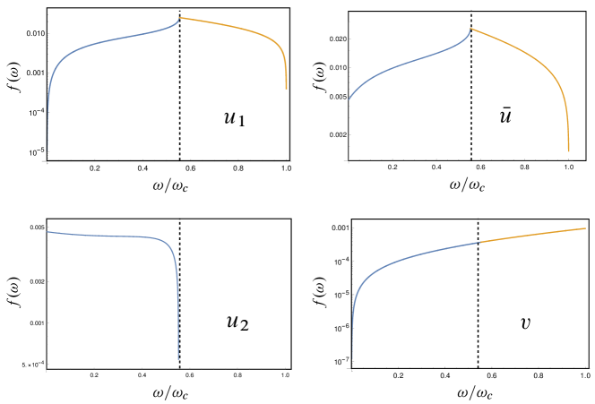
Figure 5: Power spectrums of created particles for the subsonic case. $\omega_{\text{GVH}}/\omega_{c}=0.554$ for the present parameters. Across $\omega=\omega_{\text{GVH}}$, the number of modes changes from four to three and the spectrums of $u_{1},\bar{u},u_{2}$ are not smooth at $\omega_{\text{GVH}}$.

Although there is no sonic horizon in this case, the effective temperature becomes constant above $\omega_{\text{GVH}}$ and indicates thermal property related to the GVH of emitted radiation around this frequency region (Fig. 6).

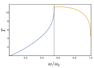
Figure 6: Effective temperature of $u_{1}$-particle for the subsonic case. Around $\omega\sim\omega_{\text{GVH}}$, the effective temperature becomes constant which indicates approximate thermal property of the radiation related to the GVH. In this plot, we adopt $c_{i}=12.57$ in Eq. (66).

V.1.2 Transsonic case

In this case, the power spectrum in the low frequency region is

$$|\beta_{u_{1}\bar{u}}|^{2}\sim\frac{(V_{+}+1)^{3/2}(V_{-}+1)(V_{+}+V_{-})}{\sqrt{1-V_{+}}\,(-V_{-}+1)(V_{+}-V_{-})}\frac{k_{0}}{\omega},\quad\omega/k_{0}\ll 1.$$ (68)

Figure 7 shows power spectrums of emitted radiations in this case. In the low frequency region, spectrums of $u_{1},\bar{u}$-particles are thermal and they decrease rapidly near the cutoff frequency $\omega_{c}$. The number of the $v$-particle shows the similar behavior as that for the subsonic case.

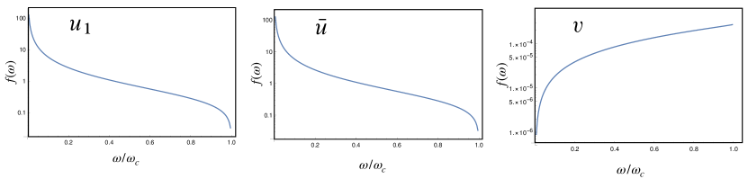
Figure 7: Power spectrums for the transsonic case.

Figure 8 shows behavior of the effective temperature for $u_{1}$-particle. Around $\omega\sim 0$, it becomes constant which reflects the thermal property of emitted radiation.

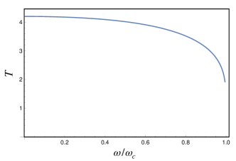
Figure 8: Effective temperature of $u_{1}$-particle for the transsonic case. Around $\omega\sim 0$, the effective temperature becomes constant. In this plot, we adopt $c_{i}=1$ in Eq. (66).

For the transsonic case with $\omega\sim 0$, neglecting contribution of $v$-mode, the Bogoliubov coefficients satisfy $|\beta_{u_{1}u_{2}}|^{2}-|\beta_{u_{1}\bar{u}}|^{2}\approx 1$. These coefficients diverge as $1/\omega$. Using this relation, the power spectrum of $u_{1}$-particle is

$$|\beta_{u_{1}\bar{u}}|^{2}\approx\left(\left|\frac{\beta_{u_{1}u_{2}}}{\beta_{u_{1}\bar{u}}}\right|^{2}-1\right)^{-1}.$$ (69)

The ratio $|\beta_{u_{1}u_{2}}/\beta_{u_{1}\bar{u}}|$ determines the power spectrum of $u_{1}$-particle. As $\omega\to 0$ the ratio $|\beta_{u_{1}u_{2}}/\beta_{u_{1}\bar{u}}|$ goes to 1 for the trans-sonic case, this behavior of the the Bogoliubov coefficients is originated from the boundary condition for the decaying wave function in $x<0$ (see Appendix B for details). The ratio can be approximated as

$$\left|\frac{\beta_{u_{1}u_{2}}}{\beta_{u_{1}\bar{u}}}\right|\simeq 1+\gamma\,\omega\approx e^{\gamma\omega},$$ (70)

where $\gamma$ is a factor determined by $V_{\pm}$. This approximation indicates that the power spectrum of $u_{1}$-particle shows thermal distribution with effective temperature $T=1/(2\gamma)$ in the low frequency range. Using (68), the temperature is given by

$$T(\omega=0)=\frac{(V_{+}+1)^{3/2}(V_{-}+1)(V_{+}+V_{-})}{\sqrt{1-V_{+}}\,(-V_{-}+1)(V_{+}-V_{-})}\,k_{0}.$$ (71)

This formula provides a numerical value of the temperature as $T(\omega=0)=4.20$ for present parameters and is consistent with the numerical result (Fig. 8). However, this temperature seems to be nothing to do with the surface gravity of the horizon because it diverges for the step velocity profile, and the thermal property appears due to non-linear dispersion relation (the Planckian mode). Indeed, the temperature (71) can be regarded as corresponding to the effective surface gravity which is defined by velocity difference divided by the effective thickness of the sonic horizon determined by the cutoff wave number $k_{0}$.

V.2 Entanglement Structure

V.2.1 Subsonic case

To analyze entanglement between each particle mode, we calculated parameters $r,\theta,\phi$ introduced in the previous section. These parameters determine components of the covariance matrix for the vacuum state. Figure 9 shows behavior of these parameters for the sub-sonic case. The squeezing parameter $r$ increases with the increase of frequency until $\omega_{\text{GVH}}$, and then decreases with the increase of $\omega$. The mixing parameters $\theta$ and $\phi$ go to zero as $\omega\to 0$, and increase with the increase of $\omega$. Thus from the definition of parameters (43), $u_{2}$-particle (Plankian mode) is mainly created for $\omega\to 0$. As $\omega$ increases, the number of $u_{1}$-particle increases until $\omega_{\text{GVH}}$. For $\omega_{\text{GVH}}<\omega$, as the GVH is formed, creation of $u_{2}$-particle is shut down and $u_{1}$-particle and $\bar{u}$-particle mainly contribute as created particles.

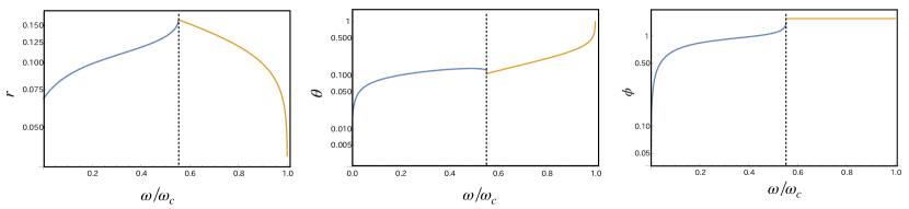
Figure 9: Behavior of parameters $r,\theta,\phi$ for the subsonic case.

Behavior of the entanglement negativity for the subsonic case is shown in Fig. 10, Fig. 11 and Fig. 12. Figure 10 is the negativity for bi-partitioning of the total pure system (four modes for $\omega<\omega_{\text{GVH}}$ (left panel) and three modes for $\omega_{\text{GVH}}<\omega$ (right panel)). For $\omega<\omega_{\text{GVH}}$, entanglement between $u_{1},v$-particles and other particles goes to zero as $\omega\to 0$. This decrease of entanglement corresponds to the decrease of the created number of $u_{1}$-particle and $v$-particle. Entanglement between $\bar{u},v,u_{1}$-particles and other particles increases with the increase of $\omega$, whereas entanglement between $u_{2}$-particle and other particles decreases. For $\omega_{\text{GVH}}<\omega$ where the GVH exists, $u_{2}$-particle disappears and the total number of modes becomes three. Entanglement between $\bar{u},u_{1}$-particles and other particles decreases and entanglement between $v$-particle and other particles increases with the increase of $\omega$.

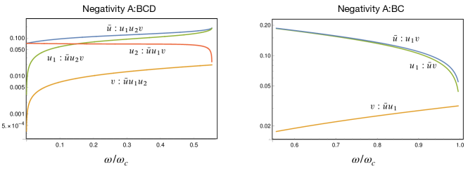
Figure 10: Negativity for the subsonic case. For low frequency $\omega<\omega_{\text{GVH}}$ (left panel), the number of particle modes is four. For high frequency $\omega_{\text{GVH}}<\omega$ (right panel), the number of particle modes is three.

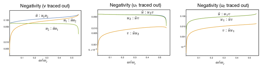
Figure 11: Negativity of reduced state for the subsonic case in the low frequency region $0<\omega<\omega_{\text{GVH}}$.

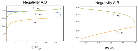
Figure 12: Negativity of reduced two mode state for the subsonic case.

In the limit of $\omega\rightarrow 0$, $u_{1}$ and $v$ modes are separable from other three modes, and $u_{2}$ and $\bar{u}$ mode forms an entangled pair. With the increase of frequency, entanglement between $u_{1}$ and $\bar{u}$ modes, and entanglement between $v$ and $\bar{u}$ modes become larger. And near the frequency $\omega_{\text{GVH}}$, entanglement between $u_{1}$ and $\bar{u}$ modes becomes the main contribution to entanglement of the four modes system. For $\omega>\omega_{\text{GVH}}$, entanglement between $u_{1}$ and $\bar{u}$ modes starts to decrease, whereas entanglement between $v$ and $\bar{u}$ modes keeps increase and their amount become comparable near the cutoff frequency $\omega_{c}$. We present schematic pictures of the entanglement structure in Fig. 13.

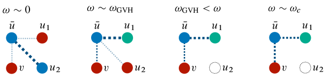
Figure 13: Schematic pictures of entanglement structure for the subsonic case. Red disks represent non-Planckian modes, blue disks represent Planckian mode, and green disks represent sub-Planckian modes. For low frequency, entanglement of the system is shared mainly by $\bar{u}$-$u_{2}$ pair. For $\omega\sim\omega_{\text{GVH}}$, entanglement of the system is shared mainly by $\bar{u}$-$u_{1}$ pair.

For $\omega\sim 0$, non-Planckian modes $u_{1},v$ can not entangle with Planckian modes $u_{2},\bar{u}$. With the increase of frequency, the non-Planckian mode $u_{1}$ becomes the sub-Planckian mode, and $\bar{u}$ and $u_{1}$ are entangled. This is the reason why entanglement between $u_{1}$ and other modes gets larger with the increase of frequency in the low frequency region.

Now let us comment on the thermal property of radiation for $\omega_{\text{GVH}}<\omega$ where the GVH exists. For models with slowly varying velocity profiles, in the vicinity of the GVH, the wave number corresponding to emitted particles is expressed as

$$k(x)=\frac{\omega-2\{c_{s}(k(x_{0}))+v(x_{0})\}}{k(x_{0})\,\kappa(x-x_{0})-\{v(x_{0})+c_{s}(k(x_{0}))\}}k(x_{0}),$$ (72)

where $x_{0}$ is the location of the GVH, $\kappa$ is the first derivative of the velocity profile at the GVH, $k(x_{0})$ is the wave number at the GVH. This $x$-dependent wave number leads to the logarithmic behavior of the phase factor $S(x,t)=\int^{x}dx^{\prime}k(x^{\prime})-\omega\,t$ with a branch point $x^{\prime}_{0}=x_{0}+(v(x_{0})+c_{s}(k(x_{0})))/k(x_{0})\kappa$. Let us introduce the WKB mode function $\psi_{\pm}=\exp(iS(x,t))$ for $x\neq x^{\prime}_{0}$. Then we obtain the positive norm in-mode function $\psi_{\text{in}}(x,t)$ as

$$\psi_{\text{in}}(x,t)\sim\psi_{+}(x,t)+\exp\left(\frac{-\pi\{\omega-2(c_{s}(k(x_{0}))+v(x_{0}))\}}{\kappa}\right)\psi_{-}(x,t),$$ (73)

which is obtained by requiring that $\psi_{\text{in}}(x,t)$ is analytic in the upper half complex $x$-plane. Equation (73) implies that the wave function includes the thermal-like factor but it deviates from the Planckian distribution owing to the existence of $c_{s}(k(x_{0}))+v(x_{0})$ terms, which also have frequency dependence. The bipartite entanglement for $\omega_{\text{GVH}}<\omega$ decreases with the increase of $\omega$, which is the same behavior for the transsonic case and related to the thermal property of radiations. These considerations suggest that the similar effect appears for the steep velocity profile case and results in approximate thermal behavior for $\omega_{\text{GVH}}<\omega$.

V.2.2 Transsonic case

Figure 14 shows $\omega$ dependence of parameters $r,\theta,\phi$, and Fig. 15 shows negativity for the transsonic case. Entanglement between $\bar{u},u_{1}$ modes and other modes decreases with the increase of $\omega$, and entanglement between $v$-mode and other modes also increase with the increase of $\omega$. This behavior is consistent with that of the power spectrum; with the increase of entanglement, the number of created particles increases.

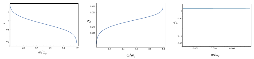
Figure 14: Frequency dependence of parameters $r,\theta,\phi$ for the transsonic case.

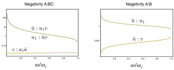
Figure 15: Behavior of negativity for the transsonic case.

For $\omega\rightarrow 0$ limit, the $v$-mode becomes approximately separable from other modes, $u_{1}$ and $\bar{u}$ are entangled. With the increase of $\omega$, entanglement between $u_{1}$ and $\bar{u}$ modes decreases and entanglement between $v$ and $\bar{u}$ modes increases. And the amount of these entanglement becomes comparable near the cutoff frequency $\omega_{c}$. This behavior is same as that observed in our previous study for the transsonic flow with finite surface gravity at the sonic horizon [8]. Schematic structure of entanglement for the transsonic case is shown in Fig. 16.

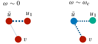
Figure 16: Schematic pictures of entanglement structure for the transsonic case. Red disks represent non-Planckian modes, blue disks represents Planckian modes, and green disks represents sub-Planckian modes. For low frequency, entanglement of the system is shared maily by $\bar{u}$-$u_{1}$ pair.

VI Conclusion

We have calculated the power spectrum and entanglement of the scalar field modes in the dispersive media with a step velocity profile. For the transsonic case, we have obtained the similar result as [8], but the temperature of the radiation is given by Eq. (71), which is not equal to derivative of the fluid velocity at the sonic horizon. For the subsonic case, the situation is completely different. Entanglement between $u_{1}$-mode and $\bar{u}$-mode, and the power spectrum of created $u_{1}$-particle increases with frequency $\omega$ until the frequency reaches $\omega_{\text{GVH}}$ where the GVH appears. The power spectrum becomes a decreasing function of frequency for $\omega_{\text{GVH}}<\omega$. For the dispersive model investigated in this paper, the power spectrum of $u_{1}$-mode for the subsonic case and for the transsonic case have the similar behavior in the high frequency region; it is not possible to distinguish them if we only measure the power spectrum for high energy particles emitted from the step. Concerning entanglement structure, we found that Planckian modes can not entangle with non-Planckian modes (see Fig. 13 and Fig. 16); For the subsonic case, in the low frequency limit, $u_{1}$-mode and $v$-mode are non-Planckian modes, and $\bar{u}$-mode and $u_{2}$-mode are Planckian modes. Entanglement of the system is shared only between $u_{2}$-mode and $\bar{u}$-mode, and the $u_{1}$-particle is not created. With the increase of frequency, $u_{1}$-mode becomes sub-Planckian mode and $u_{1}$-particle can be created. For the transsonic case, all of the modes are sub-Planckian modes in the low frequency limit, and $u_{1}$-mode and $\bar{u}$-mode can entangle.

Although we did not treat in this paper, we are interested in the following issues; the first one is how the cutoff scale affects the total energy and the total entanglement of modes. We do not understand how the total energy of modes and entanglement shared between modes with non-linear dispersions. The second one is behavior of two point correlation functions. Two point correlation functions for analog black holes are investigated in [21, 22]. It may be interesting to evaluate them for the subsonic case without a sonic horizon. The third one is dependence of dispersion relation on particle creations and entanglement. We considered the subluminal dispersion in this paper, but for the superluminal dispersion, the number of the negative norm modes is different and we expect different entanglement structure. These problems are left for our future research.

Appendix A Entanglement negativity

Entanglement of the in-vacuum state is evaluated using the positive partial transpose (PPT) criterion for continuous variable [23, 24, 25]. The PPT criterion states that if a partially transposed density matrix has negative eigen values, the bipartite state is entangled. For bosonic systems, we can rewrite the PPT criterion in terms of a covariance matrix. From positive definiteness of the density matrix and the uncertainty relation, the covariance matrix which represents a physical state should satisfy

$$V+\frac{i}{2}\,\Omega\geq 0,$$ (74)

where the inequality of the matrix stands for positive definiteness of the matrix [26]. With this property of a physical density matrix, the PPT criterion is equivalent to the following statement: If the state is separable, the covariance matrix $\widetilde{V}$ with the partially transposed density matrix satisfies

$$\widetilde{V}+\frac{i}{2}\,\Omega\geq 0.$$ (75)

The covariance matrix $\widetilde{V}$ is easily calculated by inverting the sign of the momentum $p_{i}\to-p_{i}$, which corresponds to partially transposition of a mode [25]. By diagonalization of $\widetilde{V}$ using a symplectic matrix $S_{d}$,

$$\widetilde{V}+\frac{i}{2}\,\Omega=S_{d}^{T}\left(\bigoplus_{i}\begin{pmatrix}\kappa_{i}&i/2\\ -i/2&\kappa_{i}\end{pmatrix}\right)S_{d},$$ (76)

where $\{\kappa_{i}\}$ are symplectic eigenvalues of $\widetilde{V}$. If all of the symplectic eigenvalues are greater than $1/2$, $\widetilde{V}+(i/2)\Omega$ is positive definite. To quantify entanglement, the negativity is defined by

$$N=\frac{1}{2}\,\text{max}\left[\left(\prod_{\kappa_{i}<1/2}\dfrac{1}{2\kappa_{i}}\right)-1,0\right]$$ (77)

and the logarithmic negativity $L_{N}:=\log(2N+1)$. If $N>0$ or $L_{N}>0$, the bipartite state is entangled. Logarithmic negativity is entanglement monotone (does not increase under the LOCC) and additive, thus logarithmic negativity can be used as a entanglement measure [27, 28].

Appendix B power spectrum in low frequency region

For the trans-sonic case, we expand the Bogoliubov coefficients as a power series of $\omega$ by comparing the same order terms in the both sides of the matching formula. For simplicity, we neglect the $uv$-mixing. The linear combination of the $u_{1}$-mode, $u_{2}$-mode, and $\bar{u}$-mode is chosen so that it decays exponentially as $x\rightarrow-\infty$. We consider wave functions $A\exp{ik^{-}_{\text{decay}}\,x}$ for $x<0$ and $\exp{ik^{+}_{u_{1}}\,x}+B\exp{ik^{+}_{u_{2}}\,x}+C\exp{ik^{+}_{\bar{u}}\,x}$ for $x>0$, and match them at $x=0$. The matching formula corresponding to Eq. (21) is written as

$$A=1+B+C,\quad A\,k^{-}_{\text{decay}}=k^{+}_{u_{1}}+B\,k^{+}_{u_{2}}+C\,k^{+}_{\bar{u}},\quad A(k^{-}_{\text{decay}})^{2}=(k^{+}_{u_{1}})^{2}+B(k^{+}_{u_{2}})^{2}+C(k^{+}_{\bar{u}})^{2}.$$ (78)

We expand $A,B,C$ in the power of $\omega$ as

$$A=A^{(0)}+A^{(1)}\omega+\cdots,\quad B=B^{(0)}+B^{(1)}\omega+\cdots,\quad C=C^{(0)}+C^{(1)}\omega+\cdots.$$ (79)

We substitute Eq. (79) into Eq. (78), and equate terms with the same powers of $\omega$. Wave numbers $k^{-}_{\text{decay}},k^{+}_{u_{1}},k^{+}_{u_{2}},k^{+}_{\bar{u}}$ are determined as solutions of the dispersion relation Eq. (4) as

$$k^{-}_{\text{decay}} =ik_{0}\sqrt{V_{-}^{2}-1}+\left(\frac{d\Omega}{dk}\right)^{-1}\omega+\cdots,\quad k^{+}_{u_{2}}=k_{0}\sqrt{1-V_{+}^{2}}+\left(\frac{d\Omega}{dk}\right)^{-1}\omega+\cdots,$$

$$k^{+}_{\bar{u}} =k_{0}\sqrt{1-V_{+}^{2}}+\left(\frac{d\Omega}{dk}\right)^{-1}\omega\cdots,\quad\quad k^{+}_{u_{1}}=\frac{\omega}{1-V_{+}}.$$

By substituting these expressions into Eq. (78), we obtain coefficients of the wave function in the lowest order of $\omega$ as

$$A^{(0)} =1-\frac{V_{-}^{2}-1}{V_{-}^{2}-V_{+}^{2}},$$ (80)

$$B^{(0)} =-\frac{1}{2}\left(\frac{V_{-}^{2}-1}{V_{-}^{2}-V_{+}^{2}}-i\sqrt{\frac{V_{-}^{2}-1}{1-V_{+}^{2}}}\left(1+\frac{V_{-}^{2}-1}{V_{-}^{2}-V_{+}^{2}}\right)\right),$$ (81)

$$C^{(0)} =-\frac{1}{2}\left(\frac{V_{-}^{2}-1}{V_{-}^{2}-V_{+}^{2}}+i\sqrt{\frac{V_{-}^{2}-1}{1-V_{+}^{2}}}\left(1+\frac{V_{-}^{2}-1}{V_{-}^{2}-V_{+}^{2}}\right)\right).$$ (82)

In the zeroth order of $\omega$, $N^{+}_{u_{2}}=N^{+}_{\bar{u}},~{}|\alpha_{u_{1}u_{2}}/\alpha_{u_{1}\bar{u}}|=|\beta_{u_{1}u_{2}}/\beta_{u_{1}\bar{u}}|=|B^{(0)}/C^{(0)}|=1$ holds.

References

- Hawking [1975] S. W. Hawking, Particle Creation by Black Holes, Commun. Math. Phys. 43, 199 (1975), [Erratum: Commun.Math.Phys. 46, 206 (1976)].
- Hawking [1974] S. W. Hawking, Black hole explosions, Nature 248, 30 (1974).
- Bekenstein [1973] J. D. Bekenstein, Black holes and entropy, Phys. Rev. D 7, 2333 (1973).
- Page [1993] D. N. Page, Information in black hole radiation, Phys. Rev. Lett. 71, 3743 (1993).
- Busch and Parentani [2014] X. Busch and R. Parentani, Quantum entanglement in analogue Hawking radiation: When is the final state nonseparable?, Phys. Rev. D 89, 105024 (2014).
- Bruschi et al. [2013] D. E. Bruschi, N. Friis, I. Fuentes, and S. Weinfurtner, On the robustness of entanglement in analogue gravity systems, New Journal of Physics 15, 113016 (2013).
- Isoard et al. [2021] M. Isoard, N. Milazzo, N. Pavloff, and O. Giraud, Bipartite and tripartite entanglement in a bose-einstein acoustic black hole, Phys. Rev. A 104, 063302 (2021).
- Nambu and Osawa [2021] Y. Nambu and Y. Osawa, Tripartite entanglement of Hawking radiation in dispersive model, Phys. Rev. D 103, 125007 (2021).
- Jacobson [1991] T. Jacobson, Black-hole evaporation and ultrashort distances, Phys. Rev. D 44, 1731 (1991).
- Brout et al. [1995] R. Brout, S. Massar, R. Parentani, and P. Spindel, Hawking radiation without trans-planckian frequencies, Phys. Rev. D 52, 4559 (1995).
- Unruh [1981] W. G. Unruh, Experimental black-hole evaporation?, Phys. Rev. Lett. 46, 1351 (1981).
- Unruh [1995] W. G. Unruh, Sonic analogue of black holes and the effects of high frequencies on black hole evaporation, Phys. Rev. D 51, 2827 (1995).
- Unruh and Schützhold [2005] W. G. Unruh and R. Schützhold, Universality of the Hawking effect, Phys. Rev. D 71, 024028 (2005).
- Leonhardt and Robertson [2012] U. Leonhardt and S. Robertson, Analytical theory of Hawking radiation in dispersive media, New Journal of Physics 14, 053003 (2012).
- Mayoral et al. [2011] C. Mayoral, A. Fabbri, and M. Rinaldi, Steplike discontinuities in Bose-Einstein condensates and Hawking radiation: Dispersion effects, Phys. Rev. D 83, 124047 (2011).
- Robertson [2012] S. J. Robertson, The theory of Hawking radiation in laboratory analogues, Journal of Physics B: Atomic, Molecular and Optical Physics 45, 163001 (2012).
- Corley and Jacobson [1996] S. Corley and T. Jacobson, Hawking spectrum and high frequency dispersion, Phys. Rev. D 54, 1568 (1996).
- Corley [1997] S. Corley, Particle creation via high frequency dispersion, Phys. Rev. D 55, 6155 (1997).
- Finazzi and Parentani [2012] S. Finazzi and R. Parentani, Hawking radiation in dispersive theories, the two regimes, Phys. Rev. D 85, 124027 (2012).
- Coutant et al. [2012] A. Coutant, R. Parentani, and S. Finazzi, Black hole radiation with short distance dispersion, an analytical -matrix approach, Phys. Rev. D 85, 024021 (2012).
- Schützhold and Unruh [2010] R. Schützhold and W. G. Unruh, Quantum correlations across the black hole horizon, Phys. Rev. D 81, 124033 (2010).
- Steinhauer [2015] J. Steinhauer, Measuring the entanglement of analogue Hawking radiation by the density-density correlation function, Phys. Rev. D 92, 024043 (2015).
- Peres [1996] A. Peres, Separability criterion for density matrices, Phys. Rev. Lett. 77, 1413 (1996).
- Horodecki [1997] P. Horodecki, Separability criterion and inseparable mixed states with positive partial transposition, Phys. Lett. A 232, 333 (1997).
- Simon [2000] R. Simon, Peres-horodecki separability criterion for continuous variable systems, Phys. Rev. Lett. 84, 2726 (2000).
- Simon et al. [1994] R. Simon, N. Mukunda, and B. Dutta, Quantum-noise matrix for multimode systems: U(n) invariance, squeezing, and normal forms, Phys. Rev. A 49, 1567 (1994).
- Vidal and Werner [2002] G. Vidal and R. F. Werner, Computable measure of entanglement, Phys. Rev. A 65, 032314 (2002).
- Plenio and Virmani [2005] M. B. Plenio and S. Virmani, An introduction to entanglement measures, arXiv: quant-ph/0504163 (2005).