Consensus of networked double integrator systems under sensor bias

Abstract

A novel distributed control law for consensus of networked double integrator systems with biased measurements is developed in this article. The agents measure relative positions over a time-varying, undirected graph with an unknown and constant sensor bias corrupting the measurements. An adaptive control law is derived using Lyapunov methods to estimate the individual sensor biases accurately. The proposed algorithm ensures that position consensus is achieved exponentially in addition to bias estimation. The results leverage recent advances in collective initial excitation based results in adaptive estimation. Conditions connecting bipartite graphs and collective initial excitation are also developed. The algorithms are illustrated via simulation studies on a network of double integrators with local communication and biased measurements.

I Introduction

Consensus of networked double integrators has been studied extensively in control literature and several globally convergent controllers have been proposed [1, 2, 3, 4, 5]. This degree of interest is because the double integrator is one of the most fundamental block in any control system. Applications of double integrators include feedback linearizable nonlinear mechanical and aerospace systems such as free-rigid body motion, manipulator motion and spacecraft rotation. The consensus algorithms thus obtained can be further extended to complex nonlinear systems. Multi-agent systems with double integrator dynamics have been extensively studied in literature. See for example [6] and references therein. A comprehensive survey of the several consensus results in literature can be found in [7]. The preceding references, however, assume perfect measurements or extraneous disturbances only.

The motivation for the problem of consensus under sensor bias originates from mechanical systems that have only relative position and absolute velocity measurements available for feedback. However, relative position sensors suffer from errors such as bias in measurements. Unknown biases can appear during the functioning of various sensors such as rate gyros, accelerometers, magnetometers, altimeters, range sensors etc. These biases can be an outcome of inaccurate sensor calibration, environmental conditions, etc. The presence of bias deteriorates the performance of control laws on the network, and may result in stability issues [8, 9, 10]. Specifically, bias in relative position feedback could drive the agents to infinity, if not compensated. It is, therefore, of interest to estimate the biases and possibly nullify their effect on the network. In the context of the continuous system, bias uncertainties in measurements are in general, sparsely studied. In the context of a single rigid-body system, ‘gyro bias’ is the most commonly addressed bias uncertainty and has been studied in detail in several references, including [11, 12, 13]. However, the literature on adaptive estimation and compensation of ‘position’ sensor bias is somewhat limited and the only relevant contributions known to the authors are by [14, 15]. There have of course been parallel approaches using non-smooth control laws, where disturbance rejection is possible for both single and networked second-order systems subject to knowledge of bounds on the bias uncertainty which is then modeled as a bounded disturbance. Such non smooth laws for disturbance rejection in double integrator systems have been explored in [16, 17, 18, 19]. An approach to estimating measurement inconsistencies using an output regulation-based technique is presented in [20]. Accurate estimation in [20], however requires a unique constant, graph structure.

For uncertain networked double integrators (sensor bias being one such uncertainty), conventional adaptive control laws (including [21, 22, 23, 24, 25]) require the regressor function to be persistently exciting (PE) or collectively persistently exciting(C-PE) for parameter convergence. Recently, several methods have been proposed to get rid of the PE condition for parameter convergence. [26] proposes an adaptive algorithm that uses both instantaneous state data and past measurements for the adaptation process. This scheme ensures parameter estimation errors converge to zero exponentially, subject to the satisfaction of a finite-time excitation condition. In the same spirit, [27] proposes a PI-like (Proportional-Integral controllers) parameter update law that guarantees parameter convergence with a relaxation of the PE condition, namely initial excitation (IE) on the regressor. [28] is an extension of [27], where the authors develop a distributed composite adaptive synchronization algorithm for multiple uncertain Euler-Lagrange (EL) systems to ensure parameter convergence using the collective-IE (C-IE) condition. The method proposed in [27] obviates the need for data-storage and memory allocation required in concurrent learning-based adaptive control [29] methods.

There have been several strides in consensus under bounded disturbance and zero-mean noise. In [30], a leader-follower consensus control for a network of double integrators is proposed for follower measurements corrupted by (zero-mean) noise. This control law ensures that consensus tracking is achieved in the mean square sense for both fixed and switching communication networks. However, no bias errors are accounted for in this work. [31] shows a Kalman filter inspired technique for consensus which is input to state stable. As would be expected, the accuracy of the cooperation objective is directly related to the power level of the communication noise. [32] analyzes the asymptotic properties of linear consensus algorithms in the presence of bounded measurement errors. Here, consensus is not guaranteed with respect to all possible noise realizations. In [33], a novel self-triggering co-ordination scheme for finite time consensus is proposed in the presence of unknown but bounded noise affecting the communication channels. Bias errors with unknown bounds are not the subject of study in any of the above articles.

We now summarize some of the results that lead up to the current work on consensus under measurement bias with unknown bounds. [34] proposes an adaptive control law in the presence of unknown constant bias for a double integrator network. This controller ensures bounded closed-loop signals in the presence of sensor bias which would not be the case in the absence of adaptation. However, convergence only to a neighborhood of consensus can be shown. [34] is based on the results in [14] which addresses the problem of accommodating unknown sensor bias in a direct MRAC setting for a single agent. In [35], the authors present a consensus algorithm for synchronization of double integrators over directed graphs in the presence of constant bias with unknown bounds. Here, the authors assume the existence of a bias error on each communication channel. Similar to [34], here too convergence ‘near’ a common equilibrium point is guaranteed. [36] shows an extension of [34, 35] to develop a distributed consensus tracking algorithm for spacecraft in formation modeled as an Euler-Lagrange network with similar bounded performance results. For a fixed communication graph, exact constant estimation of a constant bias and consensus in single integrator agents are demonstrated in [37]. An undirected, connected, and non-bipartite graph network is shown to be necessary and sufficient for estimation of the full bias vector.

In comparison with existing literature, the novel contributions of this article are as below.

• Adaptive control laws for exact bias estimation and consensus are developed over [34, 36, 35]. One sensor attached to each node is considered and all relative measurements from a node are assumed to be affected by the same bias in contrast to [35].

• A time-varying communication network topology is considered over [37, 34, 35, 36]. The analysis is based on jointly connected and jointly non-bipartite graphs.

• A non-bipartite property of the communication graph for a finite initial-time only is shown to be necessary in contrast to [37], where a constant non-bipartite graph is assumed for all time.

• A collective initial excitation based adaptive controller is employed for the first time in bias estimation problems over networks.

This paper is organized as follows. Section II introduces mathematical notation, necessary lemmas and in brief, graph theory. In section III, we formulate the consensus problem over a network of double integrator systems. We develop an adaptive control law for achieving consensus and bias estimation in section IV. A discussion on the choice of control gains and the collective initial excitation condition on the regressor matrix are presented in section V. Section VI presents numerical simulations validating our algorithm. Conclusions are presented in section VII.

II Preliminaries

In this section, we present several mathematical notations, lemmas, assumptions, and a concise introduction of graph theory that forms the basis of the problem formulation.

II-A Notation

$\mathbb{R}^{+}$ denotes non-negative reals. Kronecker product is denoted by $\otimes$. The Euclidean norm of a vector $x$ is denoted by $\left\lVert x\right\rVert$ and the corresponding induced matrix Euclidean norm by $\|A\|$ for a matrix $A$. A diagonal matrix with elements $d_{1},d_{2},...,d_{n}$ on the diagonal is represented by $\textrm{diag}(d_{1},...,d_{n})$. The $n\times n$ identity matrix and zero matrix are denoted by $I_{n}$ and $0_{n}$ respectively; a $n$-dimensional vector of ones is denoted $\mathbf{1}_{n}$. For a matrix $A$, the maximum and minimum eigenvalues are respectively denoted by $\lambda_{max}(A)$ and $\lambda_{min}(A)$. For a symmetric matrix $\Gamma$, the notation $\Gamma>0$ ($\Gamma<0$) is used to denote a positive-definite (negative-definite) matrix. For a matrix signal, $A(\cdot):\mathbb{R}^{+}\rightarrow\mathbb{R}^{p_{1}\times p_{2}}$, we define $\|A\|_{\infty}\triangleq\sup_{t\geq 0}\|A(t)\|$, the signal infinity norm. Time and initial condition arguments for all state variables (variables with dynamics) are uniformly omitted for notational simplicity. Similarly, function arguments for the control variables are suppressed, and they are made clear through explicit expressions proposed later in the manuscript.

II-B Graph Theory

Consider a network of $n$ agents interacting with each other over a time-varying graph. We define the interaction graph as a function of time ($t\geq 0$) through the tuple, $\mathcal{G}(t)\triangleq(\mathcal{V},\mathcal{E}(t))$, where $\mathcal{V}\triangleq{1,...,n}$ is a node set and $\mathcal{E}(t)\subseteq\mathcal{V}\times\mathcal{V}$ is an edge set signifying interaction between nodes [6] at time instant ‘$t$’. If an edge $(i,j)\in\mathcal{E}(t)$, then node $i$ is called a neighbor of node $j$ with $j$ being the head node and $i$ being the tail node indicating information flow from $i\rightarrow j$. The set of neighbors of a node $i$ at time $t$, is denoted by $\mathcal{N}_{i}(t)$. In an undirected graph, $(j,i)\in\mathcal{E}(t)\Leftrightarrow(i,j)\in\mathcal{E}(t)$ for all $i,j\in\mathcal{V}$. An undirected graph $\mathcal{G}(t)$ is instantaneously connected if there is an undirected path between every pair of distinct nodes. The adjacency matrix, $\mathbb{R}^{n\times n}\ni\mathcal{A}(t)=[a_{ij}(t)]$, is defined such that $a_{ij}(t)>0$ if $(j,i)\in\mathcal{E}(t)$ and $a_{ij}(t)=0$ if $(j,i)\notin\mathcal{E}(t)$. We assume no self edges are present and hence, $a_{ii}(t)=0$ for all $t$. For an undirected graph, $\mathcal{A}$ is symmetric. The degree matrix of the graph $\mathcal{G}$ is, $\mathcal{D}(t)\triangleq\textrm{diag}(\sum\limits_{j=1}^{n}a_{1j}(t),...,\sum\limits_{j=1}^{n}a_{nj}(t))\in\mathbb{R}^{n\times n}$ and the Laplacian matrix, $\mathcal{L}(t)\triangleq[l_{ij}(t)]\in\mathbb{R}^{n\times n}$ is computed as:

$$\mathcal{L}(t) =\mathcal{D}(t)-\mathcal{A}(t)$$

$$l_{ii}(t) =\sum\limits_{j=1,j\neq i}^{n}a_{ij}(t),\quad\quad l_{ij}(t)=-a_{ij}(t),i\neq j$$

As evident from above, $\mathcal{L}(t)$ is symmetric for undirected graphs. Further, $\mathcal{L}(t)$ has both row and column sums zero indicating that $0$ is an eigenvalue with a corresponding eigenvector being $\mathbf{1}_{n}$ (vector of ones), i.e. $\mathcal{L}(t)\mathbf{1}_{n}=\mathbf{1}_{n}^{\top}\mathcal{L}(t)=0$. Another symmetric matrix of interest is the signless Laplacian defined as $\mathcal{Q}(t)\triangleq\mathcal{D}(t)+\mathcal{A}(t)\triangleq[Q_{ij}(t)]\in\mathbb{R}^{n\times n}$ where,

$$Q_{ii}(t) =\sum\limits_{j=1,j\neq i}^{n}a_{ij}(t),\quad\quad Q_{ij}(t)=a_{ij}(t),i\neq j.$$

For an undirected graph $\mathcal{G}(t)$, both $\mathcal{L}(t)$ and $\mathcal{Q}(t)$ are positive semi-definite matrices. A union graph denoted $\cup_{\tau\in[t,t+T]}\mathcal{G}(\tau)$ is the graph formed by Adjacency matrix elements, $\bar{a}_{ij}(t)\triangleq\int_{t}^{t+T}a_{ij}(\tau)\;\textrm{d}\tau$. The union graph, as defined, is the graph obtained by collecting all the edges in the sub-graphs appearing over a time-interval $[t,t+T]$.

Definition 1.

[38] For a time-varying graph $\mathcal{G}(t)$ with adjacency matrix elements $a_{ij}(t)$, the weighted incidence matrix $\mathcal{H}:\mathbb{R}^{+}\rightarrow\mathbb{R}^{n\times\frac{n(n-1)}{2}}$ is defined as,

$$\mathcal{H}(t)\triangleq h_{ij}(t)\triangleq\begin{cases}\sqrt{a_{ij}(t)},&\text{if }e_{j}=(i,j)\\ -\sqrt{a_{ij}(t)},&\text{if }e_{j}=(j,i)\\ 0,&\quad\textrm{otherwise}\end{cases}$$

‘

Remark II.1.

In the aforementioned definition, for undirected graphs, it is standard practice to choose an arbitrary orientation (information flow direction). This has no effect on the graph Laplacian and can always be computed as, $\mathcal{L}(t)=\mathcal{H}(t)\mathcal{H}^{T}(t)$.

Definition 2.

[39] At any given time ‘$t$’, an undirected graph $\mathcal{G}(t)$ is called bipartite if there exists a disjoint partition of the node set denoted as $\mathcal{V}=\mathcal{V}_{+}(t)\cup\mathcal{V}_{-}(t)$ such that all edges in $\mathcal{G}(t)$ are between the node sets, and there are no edges within the node set. Mathematically, for all $(i,j)\in\mathcal{E}(t)$, $i\in\mathcal{V}_{k}(t)\implies j\in\mathcal{V}\setminus\mathcal{V}_{k}(t)$ for $k\in\{+,-\}$. A graph is called jointly (non-)bipartite over $[t,t+T]$ if the corresponding union graph $\cup_{\tau\in[t,t+T]}\mathcal{G}(\tau)$ is (non-)bipartite.

Remark II.2.

The above definition implies that the graph need not necessarily be (non-)bipartite for all time instants between $[t,t+T]$, but the graph obtained by collecting all the edges in the sub-graphs appearing over the time interval is (non-)bipartite.

Definition 3.

[38] The time-varying graph $\mathcal{G}(t)$ is termed jointly $(\delta,T)$-connected if there are two real numbers $\delta>0$ and $T>0$ such that the edges $(j,i)$ satisfying,

$$\int_{t}^{t+T}a_{ij}(s)\;\textrm{d}s\geq\delta,\quad i,j\in\mathcal{V}$$

form a connected graph over $\mathcal{V}$ for all $t\geqslant 0$.

Definition 4.

(Persistence of Excitation) A locally integrable function $\phi:\mathbb{R}^{+}\rightarrow\mathbb{R}^{n\times m}$ is said to be persistently exciting if there exist positive constants $\mu_{1},\mu_{2}$, and $T$ such that,

$$\mu_{1}I_{n}\leqslant\int_{t}^{t+T}\phi(\tau)\phi^{\top}(\tau)\;\textrm{d}\tau\leqslant\mu_{2}I_{n},\quad\forall t\geq 0$$

Definition 5.

[27] (Initial Excitation) A locally integrable function $\phi:\mathbb{R}^{+}\rightarrow\mathbb{R}^{p\times q}$ is said to be initially exciting if there exist constants $\bar{T}$, $\eta$ $>0$ such that,

$$\int_{t_{0}}^{t_{0}+\bar{T}}\phi^{\top}(\tau)\phi(\tau)\;\textrm{d}\tau\geqslant\eta I_{q},\quad\text{some }t_{0}\geq 0$$

The extension of persistence and initial excitation conditions to multi-agent systems are termed collective persistence of excitation (C-PE) and collective initial excitation (C-IE) respectively [28]. These are defined below.

Definition 6.

A set of bounded, locally integrable signals $\phi_{i}:\mathbb{R}^{+}\rightarrow\mathbb{R}^{r\times s}$, $\forall i=\{1,...,n\}$, are C-PE, if there exist constants $T>0$ and $\gamma>0$ such that,

$$\int_{t}^{t+T}\sum_{i=1}^{n}\phi_{i}(\tau)\phi_{i}(\tau)^{\top}d\tau\geq\gamma I_{r},\quad\forall t\geq t_{0}\geq 0$$

Definition 7.

A set of bounded, locally integrable signals $\phi_{i}:\mathbb{R}^{+}\rightarrow\mathbb{R}^{u\times v}$, $\forall i=\{1,...,n\}$, are C-IE, if there exist constants $\bar{T}>0$ and $\gamma>0$ such that,

$$\int_{t_{0}}^{t_{0}+\bar{T}}\sum_{i=1}^{n}\phi_{i}^{\top}(\tau)\phi_{i}(\tau)d\tau\geq\gamma I_{v},\quad\text{some }t_{0}\geq 0$$

The following assumption is intrinsic to the subsequent results.

Assumption 1.

The network graph, $\mathcal{G}(t)$, is undirected and jointly $(\delta,T)$-connected for some $\delta,\,T>0$. We assume the same graph $\mathcal{G}(t)$ for both relative measurements as well as information exchange. Further, we assume existence of an $a_{M}>0$ such that $a_{ij}(t)\leqslant a_{M}$ for all $i,j\in\{1,2,\ldots,n\}$ and for all $t\geqslant 0$.

II-C Fundamental Results

We state a few results from graph theory and consensus analysis to be used subsequently.

Proposition II.1.

[39] A graph $\mathcal{G}$ is bipartite if and only if $\mathcal{G}$ has no cycle of odd length.

Proposition II.2.

[40] The smallest eigenvalue of the signless Laplacian matrix $\mathcal{Q}=\mathcal{D}+\mathcal{A}$ of an undirected and connected graph is equal to zero if and only if the graph is bipartite. In case the graph is bipartite, zero is a simple eigenvalue

The following is a re-wording of [41, Theorem 3.4].

Proposition II.3.

Consider the time-varying dynamics,

$$\dot{x}=-\sigma N(t)N^{\top}(t)x,\quad x(0)=x_{0}$$ (1)

with $N:\mathbb{R}^{+}\rightarrow\mathbb{R}^{k\times p}$ being a piecewise continuous matrix function. If $N(\cdot)$ is persistently exciting (4), then the above dynamics admits a Lyapunov function

$$V(t,x)=\frac{1}{2}x^{\top}[\pi I_{k}+S(t)]x$$

where,

$$S(t)=2\delta_{T}I_{k}-\frac{2}{T}\int_{t}^{t+T}\int_{t}^{r}N(\tau)N^{\top}(\tau)\;\textrm{d}\tau\;\textrm{d}r$$

and the positive constants $\pi,\delta_{T}$ are defined as,

$$\delta_{T}\triangleq T|N(\cdot)N^{\top}(\cdot)|_{\infty},$$

$$\pi\triangleq 1+\frac{2\sigma^{2}\delta_{T}^{3}}{\mu_{1}}.$$

Further, the states of the dynamical system (1) are uniformly exponentially stable at the origin.

The following result was established as part of the proof in [38, section IIA].

Proposition II.4.

The following hold for an undirected graph $\mathcal{G}(t)$ over $n$- nodes, with Laplacian $\mathcal{L}(t)$ and weighted incidence matrix $\mathcal{H}(t)$ (1).

• $\Big{(}\mathcal{L}(t)+\frac{\mathbf{1}_{n}\mathbf{1}_{n}^{\top}}{n}\Big{)}=\Big{(}\mathcal{H}(t)+\frac{\mathbf{1}_{n}h^{\top}(t)}{\sqrt{n}}\Big{)}\Big{(}\mathcal{H}(t)+\frac{\mathbf{1}_{n}h^{\top}(t)}{\sqrt{n}}\Big{)}^{\top}$, where $h(t)$ is unit vector in the kernel of $\mathcal{H}(t)$.

• The graph $\mathcal{G}(t)$ is jointly $(\delta,T)$-connected (3) for some $\delta,T>0$ if and only if $\Big{(}\mathcal{H}(t)+\frac{\mathbf{1}_{n}h^{\top}(t)}{\sqrt{n}}\Big{)}$ is persistently exciting (4).

III Bias Estimated Consensus

The objective of this article is to develop a distributed consensus algorithm for a network of double integrator systems in the presence of a constant unknown bias corrupting the relative measurements of position while ensuring estimation of all biases by each agent. The interaction between the agents is modeled by an undirected and jointly $(\delta,T)$-connected graph, $\mathcal{G}(t)$, with an associated Laplacian $\mathcal{L}(t)$. The input-output model for each agent representing a node in $\mathcal{G}(t)$ is expressed as the following double integrator equation,

$$\ddot{q}_{i}=u_{i},$$

$$q_{i}(0)=q_{i0};\,\dot{q}_{i}(0)=\dot{q}_{i0};\,i=1,2,\ldots,n$$

$$y_{i}=[z_{ij},\;\dot{q}_{i}]^{\top},\quad i=1,2,\ldots,n,\,j\in\mathcal{N}_{i}(t)$$ (2)

where state $q_{i}\,\in\,\mathbb{R}^{m}$ is the vector of generalized coordinates (called ‘positions’ in general with their derivatives being ‘velocities’), $u_{i}(\cdot)\in\mathbb{R}^{m}$ is a distributed, time-varying feedback, $y_{i}=[z_{ij},\;\dot{q}_{i}]\,\in\,\mathbb{R}^{2m}$ is the information state available to each agent with $\mathbb{R}^{m}\ni z_{ij}\triangleq(q_{i}-q_{j}+b_{i})$ and $b_{i}\,\in\,\mathbb{R}^{m}$ is the constant, unknown sensor bias. The estimate of sensor bias ($b_{i}$) for each agent $k$ will be denoted $\hat{b}_{i}^{k}$ in the sequel. Each agent $k$ has an estimate of all sensor biases ($\hat{b}^{k}=[\hat{b}_{1}^{k},\hat{b}_{2}^{k},\ldots,\hat{b}_{n}^{k}]^{\top})$ and a dynamic update law is designed for the same.

The control objective in this article is to design a distributed feedback $u_{i}$ so that the closed-loop solutions of (III) satisfy,

$$\lim_{t\to\infty}(q_{i}-q_{j})=0,\quad\forall i,j\in\{1,2,\ldots,n\}$$

$$\lim_{t\to\infty}\dot{q}_{i}=0\quad\forall i\in\{1,2,\ldots,n\}$$

$$\lim_{t\to\infty}(b_{i}-\hat{b}_{i}^{k})=0\quad\forall i,k\in\{1,2,\ldots,n\}$$ (Bias Estimated Consensus)

The following assumption delineates the information available for the design of the feedback law $u_{i}$.

Assumption 2.

Agents can measure their own velocities ($\dot{q}_{i}$); neighbors measure relative velocities ($\dot{q}_{i}-\dot{q}_{j}$) and relative position corrupted by a constant unknown bias ($z_{ij}=q_{i}-q_{j}+b_{i}$). Further, neighbors exchange their measurement of relative positions ($z_{ji}=q_{j}-q_{i}+b_{j}$) and their estimate of biases ($\hat{b}^{j}$) with each other.

IV Control Law Design

We prescribe a controller $u_{i}$ for (III) to satisfy our control objective (Bias Estimated Consensus) where $b_{i},\,i=1,2,\ldots,n$ are assumed to be unknown, constant measurement biases.

In this article, we consider the following distributed control algorithm,

$$u_{i}=k(t)\Big{(}-\dot{q}_{i}-\frac{1}{2}\sum_{j\in\mathcal{N}_{i}}a_{ij}(t)[z_{ij}+z_{ji}]\Big{)}+w_{i}$$

where, $k:\mathbb{R}^{+}\rightarrow\mathbb{R}^{+}$ is a positive valued uniformly bounded function (there exists $k_{M}>0$ such that $k(t)\leqslant k_{M}$ for all $t\geqslant 0$) to be prescribed later, $q=[q_{1},\ldots,q_{n}]^{\top}$ and $w_{i}(\cdot)\in\mathbb{R}^{m}$ is an auxiliary control term. The implementation of the term $z_{ji}$ in the control law requires that all neighbors’ relative position measurements (corrupted by bias) be communicated to each agent. This is guaranteed by 2. The individual control expressions above can now be collected to specify the feedback for the entire double integrator network as follows:

$$u=-k(t)\dot{q}+\frac{k(t)}{2}[\mathcal{L}(t)\otimes I_{m}]b-k(t)[\mathcal{D}(t)\otimes I_{m}]b+w$$ (3)

where, $u,\;b\;\textrm{and}\;w$ are the column stacked vectors of $[u_{1},\ldots,u_{n}]^{\top}$, $[b_{1},\ldots,b_{n}]^{\top}$ and $[w_{1},\ldots,w_{n}]^{\top}$ respectively. Let $\bar{\mathcal{L}}(t)\triangleq\mathcal{L}(t)\otimes I_{m}\;\textrm{and}\;\bar{\mathcal{D}}(t):=\mathcal{D}(t)\otimes I_{m}$, then (3) can be simplified as,

$$u =-k(t)\bar{\mathcal{D}}(t)b-k(t)\dot{q}+\frac{k(t)}{2}\bar{\mathcal{L}}(t)b+w$$ (4)

We also obtain the network dynamics from (III) as,

$$\ddot{q} =u.$$ (5)

Substituting the control law (4) in (5), we obtain the following closed-loop network dynamics,

$$\ddot{q} +k(t)\dot{q}+k(t)\bigg{(}\bar{\mathcal{D}}(t)-\frac{1}{2}\bar{\mathcal{L}}(t)\bigg{)}b=w.$$ (6)

It is worth noting that $\bar{\mathcal{D}}(t)-\bar{\mathcal{L}}(t)/2=\mathcal{Q}(t)/2\otimes I_{m}\triangleq\bar{\mathcal{Q}}(t)/2$. (6) can be written in a standard regressor-parameter form as,

$$\underbrace{\Big{[}\ddot{q},\;\;k(t)\dot{q},\;\;\frac{1}{2}k(t)\bar{\mathcal{Q}}(t)\Big{]}}_{Y\in\mathbb{R}^{mn\times(mn+2)}}\underbrace{\Big{[}1\;1\;b\Big{]}^{T}}_{\theta\in\mathbb{R}^{mn+2}}=w$$

with $Y:\mathbb{R}^{m}\times\mathbb{R}^{m}\times\mathbb{R}\rightarrow\mathbb{R}^{mn\times(mn+2)}$ denoting the regressor and $\theta\in\mathbb{R}^{mn+2}$ being the constant, unknown parameter. We can also write, corresponding to each agent:

$$\small{Y_{i}=\Big{[}\ddot{q}_{i},\;\;k(t)\dot{q}_{i},\;\;\frac{1}{2}k(t)[Q_{i1}(t)I_{m},\;Q_{i2}(t)I_{m},...,\;Q_{in}(t)I_{m}]\Big{]}}.$$ (7)

$Y_{i}$ and $w_{i}$ are available for each agent, i.e., $Y_{i}\in\mathbb{R}^{m\times(mn+2)}$ corresponds to each $m$ rows of $Y$, $w_{i}\in\mathbb{R}^{m}$ corresponds to each $m$ rows of $w$. Additionally, we have corresponding to each agent, $Y_{i}\theta=w_{i}$. Each agent has an adaptive estimate of the unknown parameter vector $\theta$ for all $i=1,..,n$ (which is an over-parametrization of $b$) denoted $\hat{\theta}^{i}\in\mathbb{R}^{mn+2}$. $\hat{\theta}^{i}=[p^{i}\;l^{i}\;\hat{b}^{i}]^{\top}$ where $\hat{b}^{i}=[\hat{b}^{i}_{1},\hat{b}^{i}_{2},...,\hat{b}^{i}_{n}]^{\top}$. $p^{i}$, $l^{i}$ are the estimates of the constants in $\theta$ by agent $i$. We define the agent parameter error as, $\tilde{\theta}^{i}\triangleq[1-p^{i}\;1-l^{i}\;\tilde{b}^{i}]^{\top}$, where $\tilde{b}^{i}\triangleq[b_{1}-\hat{b}_{1}^{i},...,b_{n}-\hat{b}_{n}^{i}]^{\top}=[\tilde{b}_{1}^{i},...,\tilde{b}_{n}^{i}]^{\top}$. We now define,

$$s_{i}\triangleq\dot{q}_{i}+\lambda\bigg{(}q_{i}+\frac{\tilde{b}_{i}^{i}}{2}\bigg{)},\quad\quad\lambda>0,\,i=1,2,\ldots n$$ (8)

where $\tilde{b}_{i}^{i}\triangleq b_{i}-\hat{b}_{i}^{i}$. Further we assign, $s\triangleq[s_{1},\,\ldots,\,s_{n}]^{\top}$, $\tilde{b}_{new}\triangleq[\tilde{b}_{1}^{1},\,\ldots,\,\tilde{b}_{n}^{n}]^{\top}$ and obtain $s=\dot{q}+\lambda(q+\tilde{b}_{new}/2)$.

Note - $\tilde{b}_{i}^{i}$ has been used in eq. 8, and not $\tilde{b}_{i}^{k}$ as $\tilde{b}_{i}^{k}=b_{i}-\hat{b}_{i}^{k}$ will require bias estimate information of $b_{i}$ computed by agent $k\not\in\mathcal{N}_{i}$, which may not be available with agent $i$.
Taking the derivative of $s$ and substituting from (6),

$$\dot{s}=\ddot{q}+\lambda\bigg{(}\dot{q}+\frac{\dot{\tilde{b}}_{new}}{2}\bigg{)}$$

$$=-k(t)\dot{q}-\frac{1}{2}k(t)\bar{\mathcal{Q}}(t)b+w+\lambda\bigg{(}\dot{q}+\frac{\dot{\tilde{b}}_{new}}{2}\bigg{)}$$

$$=\underbrace{\begin{bmatrix}0_{mn\times 1}&0_{mn\times 1}&-\frac{1}{2}k(t)\bar{\mathcal{Q}}(t)\end{bmatrix}}_{Z\in\mathbb{R}^{mn\times(mn+2)}}\begin{bmatrix}1&1&b\end{bmatrix}^{\top}$$

$$-k(t)\dot{q}+w+\lambda\bigg{(}\dot{q}+\frac{\dot{\tilde{b}}_{new}}{2}\bigg{)}.$$ (9)

The corresponding dynamics for each agent $s_{i}\in\mathbb{R}^{m}$, is given by

$$\dot{s}_{i}=Z_{i}\theta-k(t)\dot{q}_{i}+w_{i}+\lambda\Big{(}\dot{q}_{i}+\frac{\dot{\tilde{b}}_{i}^{i}}{2}\Big{)}$$

where $Z_{i}\in\mathbb{R}^{m\times(mn+2)}$ is defined similar to $Y_{i}$. We now define the second part of the control, $w$ at each agent node as,

$$w_{i}=k(t)\dot{q}_{i}-Z_{i}\hat{\theta}^{i}-\lambda(\dot{q}_{i}+\frac{\dot{\tilde{b}}^{i}_{i}}{2})-\sum_{j\in\mathcal{N}_{i}}a_{ij}(t)(s_{i}-s_{j}),$$ (10)

which can be written in an implementable form as,

$$w_{i}=k(t)\dot{q}_{i}-\lambda\dot{q}_{i}-\frac{\lambda\dot{\tilde{b}}_{i}^{i}}{2}+k(t)\sum\limits_{j\in\mathcal{N}_{i}}a_{ij}(t)\hat{b}_{i}^{i}$$

$$-\sigma\sum\limits_{j\in\mathcal{N}_{i}}a_{ij}(t)(s_{i}-s_{j})-\frac{k(t)}{2}\sum\limits_{j\in\mathcal{N}_{i}}a_{ij}(t)(\hat{b}_{i}^{i}-\hat{b}_{j}^{i}),\,\sigma>0.$$ (11)

The above yields for the entire network the following,

$$w =k(t)\dot{q}-\lambda(\dot{q}+\frac{\dot{\tilde{b}}_{new}}{2})-\sigma\bar{\mathcal{L}}(t)s-Z_{new}\hat{\theta}$$ (12)

where $\hat{\theta}:=[\hat{\theta}^{1},..,\hat{\theta}^{n}]^{\top}$ and $Z_{new}(\dot{q},t)\in\mathbb{R}^{mn\times n(mn+2)}$ is defined as

$$Z_{new}(\dot{q},t)\triangleq\textrm{diag}(Z_{1}(\dot{q}_{1},t),Z_{2}(\dot{q}_{2},t),..,Z_{n}(\dot{q}_{n},t)).$$

Since the bias, $b$, is constant we have, $\dot{\tilde{b}}^{i}_{i}=-\dot{\hat{b}}_{i}^{i}$ and hence is implementable in (IV). Further, though $s_{i}$ is not implementable (due to the $(q_{i}+\tilde{b}_{i}^{i}/2)$ term in $s_{i}$), $(s_{i}-s_{j})=\dot{q}_{i}-\dot{q}_{j}+\frac{1}{2}\lambda(z_{ij}-z_{ji}-(\hat{b}_{i}^{i}-\hat{b}_{j}^{j}))$ is, and that is what appears in the control law (IV). Further, the implementation of the term $(\hat{b}_{i}^{i}-\hat{b}_{j}^{j})$ requires neighbors to exchange their bias estimates (Assumption 2).

The control law $u_{i}$ after substituting for $w_{i}$ from (IV) is given by:-

$$u_{i} =\frac{k(t)}{2}\sum_{j\in\mathcal{N}_{i}}a_{ij}(t)(\tilde{b}_{i}^{i}-\tilde{b}_{j}^{i})-\lambda\dot{q}_{i}-\frac{\lambda\dot{\tilde{b}}_{i}^{i}}{2}$$

$$-\sigma\sum_{j\in\mathcal{N}_{i}}a_{ij}(t)(s_{i}-s_{j})-k(t)\sum_{j\in\mathcal{N}_{i}}a_{ij}(t)(\tilde{b}_{i}^{i})$$

Substituting (10) in (IV),

$$\dot{s} =Z_{new}\tilde{\theta}-\sigma\bar{\mathcal{L}}(t)s$$ (13)

where $\tilde{\theta}:=[\tilde{\theta}^{1},...,\tilde{\theta}^{n}]^{\top}$, $\tilde{\theta}^{i}=\theta-\hat{\theta}^{i}$.

IV-A Bias Estimation

The matrix $Y_{i}(\dot{q}_{i},\ddot{q}_{i},t)$ in (7) is dependent on the acceleration term $\ddot{q}_{i}$ and so cannot be used in our adaptation law for bias estimation. In order to facilitate relaxation of the persistence of excitation condition, a filter is designed for each agent as proposed in [28],

$$\dot{Y}_{F_{i}} =-\beta Y_{F_{i}}+Y_{i}(\dot{q_{i}},\ddot{q_{i}},t),\quad\quad Y_{F_{i}}(0)=0$$ (14)

$$\dot{w}_{F_{i}} =-\beta w_{F_{i}}+w_{i},\quad\quad w_{F_{i}}(0)=0$$

where $\beta>0$ is the scalar filter gain, $Y_{F_{i}}\in\mathbb{R}^{m\times(mn+2)}$ and $w_{F_{i}}\in\mathbb{R}^{m}$. Solving the above equations explicitly we obtain,

$$Y_{F_{i}}(t) =e^{-\beta t}\int_{0}^{t}e^{\beta r}Y_{i}(\dot{q_{i}},\ddot{q_{i}},r)\;\textrm{d}r$$ (15)

$$w_{F_{i}}(t) =e^{-\beta t}\int_{0}^{t}e^{\beta r}w_{i}\;\textrm{d}r.$$ (16)

Utilizing the relation $Y_{i}(\dot{q}_{i},\ddot{q}_{i},t)\theta=w_{i}$ we get $Y_{F_{i}}\theta=w_{F_{i}}$ from (15) and (16). $Y_{F_{i}}$ in (14) cannot be solved explicitly as $Y_{i}(\dot{q}_{i},\ddot{q}_{i},t)$ is not measured. Therefore, we split $Y_{i}(\dot{q}_{i},\ddot{q}_{i},t)$ into measured and non-measured parts as,

$$Y_{i}(\dot{q}_{i},\ddot{q}_{i},t) =Y_{1_{i}}(\ddot{q}_{i})+Y_{2_{i}}(\dot{q}_{i},t)$$

where

$$Y_{1_{i}}(\ddot{q}_{i})=\Big{[}\ddot{q}_{i},\;\;0_{m\times 1},\;\;0_{m\times mn}\Big{]}$$

$$Y_{2_{i}}(\dot{q}_{i},t)=$$

$$\Big{[}0_{m\times 1},\;\;k(t)\dot{q}_{i},\;\;\frac{1}{2}k(t)[Q_{i1}(t)I_{m},\;Q_{i2}(t)I_{m},...,\;Q_{in}(t)I_{m}]\Big{]}$$

This implies that $Y_{F_{i}}=Y_{F_{1_{i}}}+Y_{F_{2_{i}}}$, where,

$$\dot{Y}_{F_{1_{i}}} =-\beta Y_{F_{1_{i}}}+Y_{1_{i}},\quad\quad Y_{F_{1_{i}}}(0)=0$$ (17)

$$\dot{Y}_{F_{2_{i}}} =-\beta Y_{F_{2_{i}}}+Y_{2_{i}},\quad\quad Y_{F{2_{i}}}(0)=0$$

Since $Y_{2_{i}}(\dot{q}_{i},t)$ is known, $Y_{F_{2_{i}}}$ can be solved online using (17) by employing a numerical integration scheme. We solve $Y_{F_{1_{i}}}$ analytically as follows,

$$Y_{F_{1_{i}}}(t) =e^{-\beta t}\int_{0}^{t}e^{\beta r}{Y_{1_{i}}}(\ddot{q}(r))dr$$

$$=\begin{bmatrix}e^{-\beta t}\int_{0}^{t}e^{\beta r}\ddot{q}_{i}(r)dr&0&0\end{bmatrix}$$

The elements of $Y_{F_{1_{i}}}$ can be evaluated using integration by parts as follows,

$$Y_{F_{1_{i}}}(t) =\scriptstyle{\begin{bmatrix}e^{-\beta t}[e^{\beta t}\dot{q}_{i}(t)-\dot{q}_{i}(0)]-e^{-\beta t}\int_{0}^{t}\beta e^{\beta r}\dot{q}_{i}(r)dr&0&0\\ \end{bmatrix}}$$

$$=\begin{bmatrix}\dot{q}_{i}(t)-e^{-\beta t}\dot{q}_{i}(0)-h_{i}(t)&0&0\end{bmatrix}$$

$\forall\;i=1,\cdots n$ and

$$\dot{h}_{i} =\beta\dot{q}_{i}-\beta h_{i},\quad\quad h_{i}(0)=0$$

$Y_{F_{i}}$, $w_{F_{i}}$ are filtered regressor and filtered control for each agent $i$ respectively. $Y_{F_{i}}$ can now be used in our adaptation law. Additionally, for bias estimation, we will make use of the double filtered regressor and control law introduced in [27], [28]

$$\dot{Y}_{{IF}_{i}} =Y_{F_{i}}^{\top}Y_{F_{i}},\quad\quad Y_{{IF}_{i}}(0)=0$$ (18)

$$\dot{w}_{{IF}_{i}} =Y_{F_{i}}^{T}w_{F_{i}},\quad\quad w_{{IF}_{i}}(0)=0$$ (19)

where $Y_{{IF}_{i}}\in\mathbb{R}^{(mn+2)\times(mn+2)}$, $w_{{IF}_{i}}\in\mathbb{R}^{(mn+2)}$.

Fact IV.1.

[27] Integrating (18) and (19) and using the relation $Y_{F_{i}}\theta=w_{F_{i}}$ it can be verified that,

$$Y_{{IF}_{i}}\theta=w_{{IF}_{i}},\quad\quad\forall t\geqslant 0$$ (20)

Fact IV.2.

[27] The solution $Y_{{IF}_{i}}(t)$ of (18) is a non-negative and non-decreasing function of time.

The adaptive control law for bias estimation is now chosen as,

$$\dot{\hat{\theta}}^{i} =\mu_{F}Y_{F_{i}}^{\top}(w_{F_{i}}-Y_{F_{i}}\hat{\theta}^{i})+\mu_{IF}(w_{{IF}_{i}}-Y_{{IF}_{i}}\hat{\theta}^{i})$$

$$+\sum_{j\in\mathcal{N}_{i}}a_{ij}(\hat{\theta}^{i}-\hat{\theta}^{j}),\forall i=1,..,n$$ (21)

which using IV.1 can be written as,

$$\dot{\tilde{\theta}} =-\mu_{F}\phi_{F}\tilde{\theta}-\mu_{IF}\phi_{IF}\tilde{\theta}-\mathcal{L}\otimes I_{(mn+2)}\tilde{\theta}$$ (22)

$$\dot{\hat{b}}^{i} =[\dot{\hat{\theta}}^{i}_{(3)}\,\,\dot{\hat{\theta}}^{i}_{(4)}\,\,\cdots\,\,\dot{\hat{\theta}}^{i}_{({mn+2})}]^{T}$$

for constant $\mu_{F},\;\mu_{IF}>0$ and arbitrary initial conditions. $\dot{\hat{\theta}}^{i}_{(k)}$ denotes the $k^{th}$-element of $\dot{\hat{\theta}}^{i}$ and so on. $\phi_{F},\phi_{IF}\in\mathbb{R}^{n(mn+2)\times n(mn+2)}$ are block diagonal matrices and are defined as,

$$\phi_{F} \triangleq\textrm{diag}(Y_{F_{1}}^{\top}Y_{F_{1}},...,Y_{F_{n}}^{\top}Y_{F_{n}})$$

$$\phi_{IF} \triangleq\textrm{diag}(\int_{0}^{t}Y_{F_{1}}^{\top}Y_{F_{1}},..,\int_{0}^{t}Y_{F_{n}}^{\top}Y_{F_{n}}).$$

Further, we consider the following assumption and a corresponding proposition.

Assumption 3.

The set of filtered regressors $Y_{F_{i}}$ are C-IE as per 7.

Remark IV.1.

It is worth noting that the solution $Y_{F_{i}}$ in the assumption above depends on the initial conditions of the closed-loop state $\dot{q}_{i}(0)$. The collective initial excitation condition is therefore not necessarily uniform with respect to initial data.

Proposition IV.1.

[28] Provided 3 holds, the matrix $M(t)=\mathcal{L}\otimes I_{(mn+2)}+\mu_{IF}\phi_{IF}$ appearing in (22) is uniformly strictly positive definite over the time window $[\bar{T},\infty)$ i.e.,

$$\xi^{\top}M(t)\xi>0,,\quad\quad\forall t\geq\bar{T}$$

$\forall\xi\in\mathbb{R}^{n(mn+2)}.$

We are now ready to state the primary result of this article.

Theorem IV.1.

Consider the multi-agent network with the agent dynamics given by (III) interacting over an undirected graph $\mathcal{G}(t)$. If Assumptions 1-3 hold, then the control law given by,

$$u =Z_{new}{\tilde{\theta}}-\sigma\bar{\mathcal{L}}(t)s-\lambda\dot{q}-\lambda\frac{\dot{\tilde{b}}_{new}}{2}$$

with bias adaptation law (IV-A), guarantees that $\lim\limits_{t\to\infty}(q_{i}-q_{j})=0$ (for all $i,j\in\{1,2,\ldots,n\}$), $\lim\limits_{t\to\infty}\dot{q}=0$ and $\lim_{t\to\infty}(b_{i}-\hat{b}_{i}^{k})=0$ (for all $i,k\in\{1,2,\ldots,n\}$) exponentially (beyond the collective initial excitation window, i.e. $t\geqslant\bar{T}$) for sufficiently large $\mu_{IF}>0$, while ensuring that the trajectories of the closed-loop system given by (IV), (12), and (22) are uniformly bounded.

Remark IV.2.

While the result stated in IV.1 pertains to the consensus problem, the same idea extends to the trajectory tracking problems for a known bounded, smooth trajectory $r(t)$ known to the agents. The error variable $e\triangleq(q-r)$ is used in the results and control design instead of $q$.

Proof.

The closed-loop system using (13), (22), and (20) can be written in the following matrix structure,

$$\small{\frac{\;\textrm{d}}{\;\textrm{d}t}\begin{pmatrix}s\\ \tilde{\theta}\end{pmatrix}} =\small{\begin{pmatrix}-\sigma I_{mn}&Z_{new}(\dot{q},t)\\ 0&-\mu_{F}\phi_{F}-\mu_{IF}\phi_{IF}-\mathcal{L}\otimes I_{(mn+2)}\end{pmatrix}}$$

$$\times\small{\begin{pmatrix}\bar{\mathcal{L}}(t)s\\ \tilde{\theta}\end{pmatrix}}$$

We now define a new consensus error variable $\epsilon\triangleq(I_{mn}-\frac{\mathbf{1}_{n}\mathbf{1}_{n}^{\top}}{n}\otimes I_{m})s=(s-\sum_{i=1}^{n}s_{i}/n)$. The dynamics in the new error state variables are,

$$\dot{\epsilon}=-\sigma\Big{(}\bar{\mathcal{L}}(t)+\frac{\mathbf{1}_{n}\mathbf{1}_{n}^{\top}}{n}\otimes I_{m}\Big{)}\epsilon$$

$$+\Big{(}I_{mn}-\frac{\mathbf{1}_{n}\mathbf{1}_{n}^{\top}}{n}\otimes I_{m}\Big{)}Z_{new}(\dot{q},t)\tilde{\theta}$$

$$\dot{\tilde{\theta}}=-(\mu_{F}\phi_{F}+\mu_{IF}\phi_{IF}+\mathcal{L}\otimes I_{(mn+2)})\tilde{\theta}$$ (23)

Arriving at the first equation is a straightforward application of the definition of $\epsilon$, computing its derivative according to the preceding dynamics and noting the fact that $\sigma\bar{\mathcal{L}}(t)s=\sigma\bar{\mathcal{L}}(t)(\epsilon+\frac{\mathbf{1}_{n}\mathbf{1}_{n}^{\top}}{n}\otimes I_{m}s)$; $(\frac{\mathbf{1}_{n}\mathbf{1}_{n}^{\top}}{n}\otimes I_{m})(I_{mn}-\frac{\mathbf{1}_{n}\mathbf{1}_{n}^{\top}}{n}\otimes I_{m})=0$. Similar transformation equations appear in consensus analysis in [38, section IIA].

By applying II.4 we have,

$$\Big{(}\bar{\mathcal{L}}(t)+\frac{\mathbf{1}_{n}\mathbf{1}_{n}^{\top}}{n}\otimes I_{m}\Big{)}=(N(t)\otimes I_{m})(N(t)\otimes I_{m})^{\top}$$

where $N(t)\triangleq\Big{(}\mathcal{H}(t)+\frac{\mathbf{1}_{n}h^{\top}(t)}{\sqrt{n}}\Big{)}$. It is also evident from II.4 that $N(t)$ is persistently exciting since $\mathcal{G}(t)$ is jointly $(\delta,T)$-connected. For the error dynamics (IV-A) we choose the following candidate Lyapunov function motivated by II.3,

$$V(t,\epsilon,\tilde{\theta})=\frac{1}{2}\epsilon^{\top}[\pi I_{mn}+S(t)]\epsilon+\frac{1}{2}\tilde{\theta}^{\top}\tilde{\theta}$$

where $S(t)$ and constants $\pi,\delta_{T}$ are as defined in II.3 with $N(t)$ defined above. It is immediately evident from the definition of $S(t)$ and $\delta_{T}$ that,

$$0\leqslant S(t)\leqslant 2\delta_{T}I_{mn}$$

and the derivative of $S(t)$ can be computed as,

$$\dot{S}(t)=2N(t)N^{\top}(t)-\frac{2}{T}\int_{t}^{t+T}N(\tau)N^{\top}(\tau)\;\textrm{d}\tau.$$

It is therefore obvious that $V(t,\epsilon,\tilde{\theta})\geqslant 0.5(\pi\|\epsilon\|^{2}+\|\tilde{\theta}\|^{2})$ and therefore is a positive definite function. The directional derivative of $V(t,\epsilon,\tilde{\theta})$ along the dynamics (IV-A) can now be computed as,

$$\dot{V}(t,\epsilon,\tilde{\theta})=-(\pi\sigma-1)\epsilon^{\top}N(t)N^{\top}(t)\epsilon-\sigma\epsilon^{\top}S(t)N(t)N^{\top}(t)\epsilon$$

$$-\frac{1}{T}\epsilon^{\top}\int_{t}^{t+T}N(\tau)N^{\top}(\tau)\;\textrm{d}\tau\epsilon$$

$$+\epsilon^{\top}[\pi I_{mn}+S(t)]\bar{I}_{mn}Z_{new}(\dot{q},t)\tilde{\theta}$$

$$-\tilde{\theta}^{\top}(\mu_{F}\phi_{F}+\mu_{IF}\phi_{IF}+\mathcal{L}\otimes I_{(mn+2)})\tilde{\theta}$$

where $\bar{I}_{mn}\triangleq\Big{(}I_{mn}-\frac{\mathbf{1}_{n}\mathbf{1}_{n}^{\top}}{n}\otimes I_{m}\Big{)}$ is used as a placeholder. We now compute an upper bound for $\dot{V}(t,\epsilon,\tilde{\theta})$ as below. Keeping in mind that $\phi_{F}\geqslant 0$, $\phi_{IF}\geqslant 0$ and Proposition IV.1 we obtain,

$$\dot{V}(t,\epsilon,\tilde{\theta})\leqslant-(\pi\sigma-1)\|N^{\top}(t)\epsilon\|^{2}-\frac{\mu_{1}}{T}\|\epsilon\|^{2}+\frac{\sigma\gamma}{2}\|N^{\top}(t)\epsilon\|^{2}$$

$$+\frac{\sigma}{2\gamma}\|S(t)N(t)\|^{2}\|\epsilon\|^{2}-\mu_{IF}\lambda_{min}(M(t))\|\tilde{\theta}\|^{2}$$

$$+\|[\pi I_{mn}+S(t)]\|\|\bar{I}_{mn}\|\|Z_{new}(\dot{q},t)\|\|\epsilon\|\|\tilde{\theta}\|$$

$$\leqslant-(\pi\sigma-1-\frac{\sigma\gamma}{2})\|N^{\top}(t)\epsilon\|^{2}-\big{(}\frac{\mu_{1}}{T}-\frac{\sigma}{2\gamma}\|N\|_{\infty}^{2}\|S\|_{\infty}^{2}\big{)}\|\epsilon\|^{2}$$

$$+z_{M}(\pi+\|S\|_{\infty})\|\bar{I}_{mn}\|\|\epsilon\|\|\tilde{\theta}\|-\mu_{IF}\lambda_{min}(M(t))\|\tilde{\theta}\|^{2}$$

where the first inequality is based on norm upper bounding, utilizing the persistence condition on $N(t)$ (4) and applying the Young’s inequality to bound mixed terms in $\epsilon$ using a constant $\gamma>0$. We now note that $\|S\|_{\infty}\leqslant 2\delta_{T}$ and make the following choice of constants in the above inequality,

$$\gamma=\frac{4\sigma T\delta_{T}^{2}}{\mu_{1}}\|N\|_{\infty}^{2};\quad\pi=\frac{1}{\sigma}+\frac{2\sigma T\delta_{T}^{2}}{\mu_{1}}\|N\|_{\infty}^{2}$$

which leads to,

$$\dot{V}(t,\epsilon,\tilde{\theta}) \leqslant-\frac{\mu_{1}}{2T}\|\epsilon\|^{2}+z_{M}(\pi+2\delta_{T})\|\bar{I}_{mn}\|\|\epsilon\|\|\tilde{\theta}\|$$

$$-\mu_{IF}\lambda_{min}(M(t))\|\tilde{\theta}\|^{2}$$

$$\leqslant-\big{(}\frac{\mu_{1}}{2T}-\frac{\beta}{2\gamma^{o}}\big{)}\|\epsilon\|^{2}$$

$$-\big{(}\mu_{IF}\lambda_{min}(M(t))-\frac{\beta\gamma^{o}}{2}\big{)}\|\tilde{\theta}\|^{2}$$

where the final inequality is an application of the Young’s inequality with some $\gamma^{o}>0$ and $\beta\triangleq z_{M}(\pi+2\delta_{T})\|\bar{I}_{mn}\|$. We note that $M(t)\geq M(t_{0}+\bar{T})>0$ $\forall$ $t\geq t_{0}+\bar{T}$, which implies $\exists$ $c>0$ such that $\lambda_{min}(M(t))\geq c>0$ using the argument as in IV.2. Therefore, the following choice of constants guarantees exponential convergence of the $(\epsilon,\tilde{\theta})$ dynamics to the origin.

$$\gamma^{o}>\frac{\beta T}{\mu_{1}};\quad\mu_{IF}>\frac{\beta^{2}T}{2\mu_{1}\lambda_{min}(M(t))}$$

We can now argue from the convergence of $\epsilon$ that $\bar{\mathcal{L}}(t)s\rightarrow 0$ exponentially. Now employing the definition of $s_{i}$ in (8) and accounting for the fact that $s_{i}-s_{j}\rightarrow 0$ for all $i,j\in\{1,2,\ldots,n\}$ and $\tilde{b}^{i}\rightarrow 0$ exponentially, we are left with,

$$\frac{\;\textrm{d}}{\;\textrm{d}t}(q_{i}-q_{j})=-\lambda(q_{i}-q_{j})+\Upsilon(t)$$

where $\Upsilon:\mathbb{R}^{+}\rightarrow\mathbb{R}^{m}$ denotes an exponentially decaying function. This immediately shows that $\lim_{t\rightarrow\infty}(q_{i}-q_{j})=0$ and the convergence is exponential. This implies that $(\bar{\mathcal{L}}(t)q,\;\bar{\mathcal{L}}(t)\dot{q})\rightarrow(0,0)$ exponentially, from the above equation. We use these facts to carry out an asymptotic analysis of the closed-loop by substituting $w$ from (12) in (6). Since, $\tilde{b},\dot{\tilde{b}}\rightarrow 0$, we have the dynamics, in the limit, as $\ddot{q}=-\lambda\dot{q}$, which immediately proves that $\lim_{t\rightarrow\infty}\dot{q}=0$ exponentially using similar arguments as before.
For proof of boundedness, we note that in the $\tilde{\theta}$ dynamics of (IV-A), $\mu_{F},\mu_{IF}>0$ and $\phi_{F}$, $\phi_{IF}$, $\mathcal{L}\otimes I_{(mn+2)}$ are symmetric positive semidefinite matrices at each $t\geqslant 0$. Therefore we immediately have $\|\tilde{\theta}\|\leqslant\|\tilde{\theta}(0)\|$. It is already known that the unforced ($\tilde{\theta}=0$) dynamics of $\epsilon$ is exponentially stable ([41, 38]) and from the fact that the forcing term is bounded, we can conclude boundedness of $\|\epsilon\|$ irrespective of the collective initial excitation on $Y_{F_{i}}$. Therefore $\|\bar{\mathcal{L}}(t)s\|=\|\bar{\mathcal{L}}(t)\epsilon\|$ is also uniformly bounded. Therefore, employing the definition of $s_{i}$ in (8) we obtain,

$$s_{i}-s_{j}=\dot{q}_{i}-\dot{q}_{j}+\lambda(q_{i}-q_{j})=\psi(t)$$

where $\psi:\mathbb{R}^{+}\rightarrow R^{mn}$ is a uniformly bounded function ($\|\psi(t)\|\leqslant\psi_{M}$). We have used the boundedness of $\tilde{b}$ to arrive at the above. Solving the above equation allows us to conclude that $\|(q_{i}-q_{j})\|$ and $\|(\dot{q}_{i}-\dot{q}_{j})\|$ are uniformly bounded. ∎

Remark IV.3.

We note that the first equation in the system (IV-A) is identical to the consensus dynamics studied in [41] and similar in structure to [38, section IIA] if the forcing term due to $\tilde{\theta}$ vanishes. The $\tilde{\theta}$ term is a result of the unknown sensor bias being studied in this article and evolves according to network properties embedded in $\phi_{F}$, $\phi_{IF}$, and $Z_{new}(\dot{q},t)$.

V Choosing gains and C-IE condition on regressors

A central condition for exponential convergence of the bias estimation error to zero is 3. We have, $Y_{F_{i}}(t)=e^{-\beta t}\int_{0}^{t}e^{\beta s}Y_{i}(\dot{q}_{i}(\tau),\ddot{q}_{i}(\tau),\tau)\;\textrm{d}\tau$, where from (7), $Y_{i}(\dot{q}_{i},\ddot{q}_{i},t)$ = $\Big{[}\ddot{q}_{i},\,\,k(t)\dot{q}_{i},\,\,\frac{1}{2}k(t)[Q_{i1}(t)I_{m},Q_{i2}(t)I_{m},...,Q_{in}(t)I_{m}]\Big{]}$. For 3 to be satisfied, it is required that the integral of $\sum_{i=1}^{n}Y_{F_{i}}^{\top}Y_{F_{i}}$ over the initial finite time window spans the $mn+2$ dimensional space. We will now prove that, if the set of regressors $Y_{i}$’s are C-IE then the set of filtered regressors, $Y_{F_{i}}$’s, are also C-IE which further implies that $Y_{{IF}_{i}}$’s are C-IE.

Proposition V.1.

The sufficient condition for the set of $Y_{F_{i}}$’s ($i\in\{1,2,\ldots,n\}$) to be C-IE is that the set of $Y_{i}$’s are C-IE.

Proof.

We proceed along the line of proof given in [42, Proposition 4.1]. Consider an arbitrary unit vector $v\in\mathbb{R}^{(mn+2)}$ and define the following variables:-

$$K_{i}\triangleq Y_{i}v$$

$$K_{F_{i}}\triangleq Y_{F_{i}}v$$

Let us assume that the set of regressors $Y_{i}$’s are C-IE. The above proposition can now be proved by contradiction. Suppose that $Y_{F_{i}}$’s are not C-IE. Then, $\exists$ $v\in\mathbb{R}^{(mn+2)}$ such that

$$\int_{t_{0}}^{t_{0}+T}\sum_{i=1}^{n}(K_{F_{i}}^{\top}({\tau})K_{F_{i}}(\tau))d\tau=0$$

which implies that, $K_{F_{i}}(t)=0$, $\forall i$, $\forall t\in[t_{0},t_{0}+T]$. Therefore, $\dot{K}_{F_{i}}(t)=0$ $\forall i$ and $t\in(t_{0},t_{0}+T)$. By definition, we have,

$$\dot{K}_{F_{i}}=-\beta K_{F_{i}}+K_{i}$$

which indicates that $K_{i}(t)$ is zero for all $i$, $\forall t\in(t_{0},t_{0}+T)$. This contradicts the fact that $Y_{i}$’s are C-IE. Hence, the set of $Y_{i}$’s being C-IE implies that the set of $Y_{F_{i}}$’s are C-IE. ∎

We now derive a necessary condition to be able to conclude collective Initial Excitation (C-IE) on the set of regressors, $Y_{i}(\dot{q},\ddot{q},t)$. Since, $Y=[Y_{1},Y_{2},..,Y_{n}]^{\top}$ we can write,

$$\sum_{i=1}^{n}Y_{i}^{\top}Y_{i}(\dot{q}_{i},\ddot{q}_{i},t)= Y^{\top}Y(\dot{q},\ddot{q},t)=\begin{pmatrix}A(\dot{q},\ddot{q},t)&B(\dot{q},\ddot{q},t)\\ B^{\top}(\dot{q},\ddot{q},t)&C(\dot{q},t)\end{pmatrix},$$

where, $$A(\dot{q},\ddot{q},t)=\begin{pmatrix}\ddot{q}^{\top}\ddot{q}&k(t)\ddot{q}^{\top}\dot{q}\\ k(t)\dot{q}^{\top}\ddot{q}&k^{2}(t)\|\dot{q}\|^{2}\end{pmatrix},$$

$$B(\dot{q},\ddot{q},t)=\begin{pmatrix}\frac{k(t)}{2}\ddot{q}^{\top}\bar{\mathcal{Q}}(t)\\ \frac{k^{2}(t)}{2}\dot{q}^{\top}\bar{\mathcal{Q}}(t)\end{pmatrix},$$

$$C(t)=\frac{k^{2}(t)}{4}\bar{\mathcal{Q}}(t)^{\top}\bar{\mathcal{Q}}(t).$$

All arguments in the preceding equation have been deliberately removed for the sake of brevity and clarity. The functions $A(\dot{q},\ddot{q},t)$ and $C(t)$ as defined above, map into positive semidefinite matrices by definition. We now state the result pertinent to this section.

Lemma V.1.

If $Y_{i}(\dot{q}_{i},\ddot{q}_{i},t)$’s are collectively initially exciting as per 7, then the matrix functions, $\int_{0}^{\bar{T}}A(\dot{q},\ddot{q},t)\;\textrm{d}t$ and $\int_{0}^{\bar{T}}C(t)\;\textrm{d}t$ are positive definite. Further, if the graph, $\mathcal{G}(t)$ is jointly $(\delta,T)$-connected for some $\delta>0$, then it is also jointly non-bipartite over $[0,\max\{T,\bar{T}\}]$.

Proof.

Let us assume for contradiction that $0\in\text{spec}\{\int_{0}^{\bar{T}}C(t)\;\textrm{d}t\}$. Let the eigenvalues be ordered as $0\leqslant\beta_{2}\leqslant\cdots\leqslant\beta_{mn}$. We already know that $\int_{0}^{\bar{T}}\sum_{i=1}^{n}Y_{i}^{\top}Y_{i}(\dot{q}_{i},\ddot{q}_{i},\tau)\;\textrm{d}\tau\geqslant 0$ which indicates that all eigenvalues are non-negative. Let us assume these are ordered as $\lambda_{1}\leqslant\lambda_{2}\leqslant\cdots\leqslant\lambda_{(mn+2)}$. Since $\int_{0}^{\bar{T}}C(t)\;\textrm{d}t$ is a principal submatrix of $\int_{0}^{\bar{T}}\sum_{i=1}^{n}Y_{i}^{\top}Y_{i}(\dot{q}_{i},\ddot{q}_{i},\tau)\;\textrm{d}\tau$, we can use the Cauchy’s interlacing and inclusion theorem ([43, Theorem 8.4.5]) to conclude that, $\lambda_{1}\leqslant 0\leqslant\lambda_{3}$. Since $\int_{0}^{\bar{T}}\sum_{i=1}^{n}Y_{i}^{\top}Y_{i}(\dot{q}_{i},\ddot{q}_{i},\tau)\;\textrm{d}\tau\geqslant 0$, the only possibility is $\lambda_{1}=0$. This immediately implies that the set of $Y_{i}(\dot{q}_{i},\ddot{q}_{i},t)$’s are not collectively initially exciting, thus contradicting our premise. Similar arguments can be used to claim that $\int_{0}^{\bar{T}}A(\dot{q},\ddot{q},t)\;\textrm{d}t>0$.
From $\int_{0}^{\bar{T}}C(t)\;\textrm{d}t>0$ along with the facts that $k(t)>0$, we can immediately conclude $\int_{0}^{\bar{T}}\bar{\mathcal{Q}}^{2}(t)\;\textrm{d}t\geqslant\lambda_{c}I_{mn}$ for some $\lambda_{c}>0$. This immediately implies that $\int_{0}^{\max\{T,\bar{T}\}}\bar{\mathcal{Q}}(t)\;\textrm{d}t>0$. The union graph of $\mathcal{G}(t)$, denoted $\cup_{t\in[0,\max\{T,\bar{T}\}]}\mathcal{G}(t)$, is connected by the joint $(\delta,T)$-connectedness assumption. The positive definiteness of the signless Laplacian for the union graph ($\int_{0}^{\max\{T,\bar{T}\}}\bar{\mathcal{Q}}(t)\;\textrm{d}t$) and the joint connectivity of the union graph allows us to invoke II.2 and conclude that the union graph $\cup_{t\in[0,\max\{T,\bar{T}\}]}\mathcal{G}(t)$ is non-bipartite, i.e. $\mathcal{G}(t)$ is jointly non-bipartite over $[0,\max\{T,\bar{T}\}]$. ∎

Remark V.1.

We note here that [37] utilizes the non-bipartite graph structure to propose exponential bias estimators. The graph is, however, assumed to be constant. The necessary condition above allows the use of time-varying graphs that are only jointly non-bipartite (as opposed to at each time instant) and persists only for a finite time $[0,\max\{T,\bar{T}\}]$.

Based on V.1, assuming that we have a jointly non-bipartite union graph over $[0,\max\{T,\bar{T}\}]$, the primary purpose of $k(t)$ is to ensure that $\int_{0}^{\bar{T}}A(\dot{q},\ddot{q},t)\;\textrm{d}t$ becomes positive definite. While there is no direct way to prescribe such a function for all possible initial conditions and system parameters, we introduce multiple frequency components through the time dependence in $k(t)$ to make the columns of $A(\dot{q},\ddot{q},t)$ linearly independent over sub-intervals.

VI Simulation Results

We now present simulation studies to verify IV.1 for a network of double integrators interacting via an undirected graph $\mathcal{G}(t)$ and bias corrupted measurements. We consider the translational dynamics of $n$ identical quadrotors given by

$$\ddot{q}_{i}=\begin{bmatrix}0\\ 0\\ -9.8\end{bmatrix}+\textbf{R}_{i}e_{3}\frac{\tau_{1_{i}}}{M},\quad\forall i=1,2,..,n$$ (24)

where the position vector is denoted by $q_{i}=(x_{i},y_{i},z_{i})^{\top}\in\mathbb{R}^{3}$, $e_{3}=(0,0,1)^{\top}$, $M\in\mathbb{R}^{+}$ is the mass of the quadrotor. $\textbf{R}_{i}\in SO(3)$ is the $3\times 3$ orthogonal rotation matrix from the quadrotor body frame to the inertial frame. The feedback $\tau_{1_{i}}(\cdot)\in\mathbb{R}$ is the sum of thrust forces from the individual motors in each quadrotor. Typical tracking control of the quadrotor consists of an inner loop attitude control [44] which modulates $\textbf{R}_{i}$ while the outer loop translation control is designed assuming full linear actuation in (24). Therefore, (24) can be treated as a double integrator model for our purposes by assuming a new control $u_{i}:=\textbf{R}_{i}e_{3}\frac{\tau_{1_{i}}}{M}$. For these simulations we have considered $n=5.$

Two adjacency matrices are used, one corresponding to a non-bipartite, connected graph($\mathcal{A}_{b}$) and another corresponding to a bipartite, connected graph($\mathcal{A}_{c}$).

$$\mathcal{A}_{b}=\begin{bmatrix}0&1&1&0&1\\ 1&0&1&0&1\\ 1&1&0&1&0\\ 0&0&1&0&0\\ 1&1&0&0&0\\ \end{bmatrix},\quad\mathcal{A}_{c}=\begin{bmatrix}0&1&0&0&1\\ 1&0&1&0&0\\ 0&1&0&1&0\\ 0&0&1&0&0\\ 1&0&0&0&0\\ \end{bmatrix}.$$

The graphs corresponding to $\mathcal{A}_{b}$ and $\mathcal{A}_{c}$ are shown in Figure 2 and Figure 2, respectively.

Figure 1: Connected non-Bipartite graph

Figure 2: Connected Bipartite graph

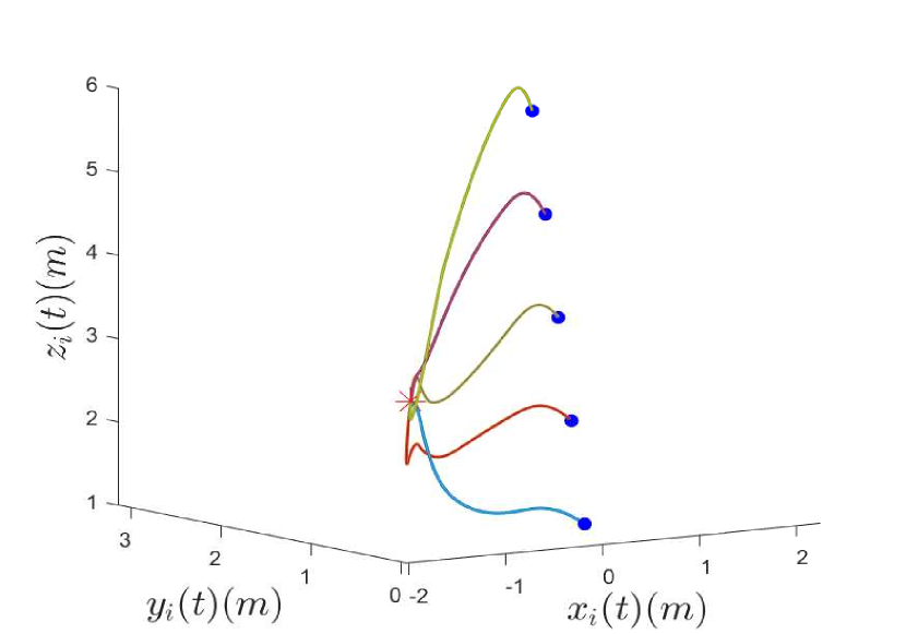
Figure 3: $x_{i}(t)(m)$ vs $y_{i}(t)(m)$ vs $z_{i}(t)(m)$. The blue dots indicate start locations, and the red asterisk the terminal locations.

The actual adjacency matrix is obtained by cycling periodically (period $T=8s$) between sub graphs of $\mathcal{A}_{b}$ for the first $t=8$ seconds and then between sub graphs of $\mathcal{A}_{c}$ for the rest of the time. This allows for a jointly non-bipartite and connected graph in the initial phase of the simulations and a jointly bipartite, connected graph beyond.

The initial position, velocity, and the bias in relative measurement of the position for the $i^{th}$ quadrotor are given by [$\frac{i\pi}{7}$; $\frac{i\pi}{5}$; $\frac{i\pi}{3}$], [$0.1i-0.7$; $-0.1i+0.6$; $0.1i+0.7$ ], [$\frac{i\pi}{12}$; $\frac{i\pi}{12}$; $\frac{i\pi}{12}$] respectively for $i=1,2,..,5$. $\hat{\theta}^{i}$ is initialized to the zero vector for $i=1,2,..,5$. The gain constants $\sigma$, $\mu_{F}$, $\mu_{IF}$, $\lambda$, and $\beta$ are chosen to be 0.2, 0.020, 15, 0.5, 0.5 respectively and $k(t)=1+0.5cos^{2}(t)+0.5sin^{2}(2t)$. The gain chosen helps introduce multiple frequency components through the time dependence in $k(t)$. The chosen $k(t)$ ensures that $\int_{0}^{\bar{T}}A(\dot{q},\ddot{q},t)\;\textrm{d}t$ becomes positive definite, which guarantees collective initial excitation on the regressor $Y_{i}$’s.

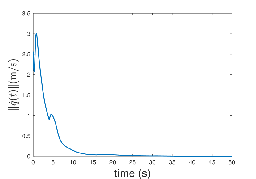
Figure 4: $\|\dot{q}(t)\|(m/s)$ vs time ($s$).

Figure 3 is the phase-plane evolution of the three positions. As is evident, starting from different initial conditions, they converge to consensus. Similarly, all the three velocities in Figure 4 and the bias estimation errors given by $\tilde{b}=[\tilde{b}^{1},\tilde{b}^{2},\tilde{b}^{3},\tilde{b}^{4},\tilde{b}^{5}]^{\top}$ in Figure 5 converge to zero during the simulation horizon. The final plot, Figure 6 is for the verification of V.1, wherein we claim that the collective initial excitation of the regressors necessitates a jointly non-bipartite graph. Figure 6 plots the determinant of $\int_{t}^{t+T}\mathcal{Q}(\tau)\;\textrm{d}\tau$ for all $t$, keeping $T=4s$ as the cycling period. We see that the $\int_{t}^{t+T}\mathcal{Q}(\tau)\;\textrm{d}\tau$ is positive definite over an initial period of time and beyond this is singular. This verifies, by II.2 that $\mathcal{G}(t)$ determined by $\mathcal{A}(t)$ is jointly non-Bipartite over a finite initial window.

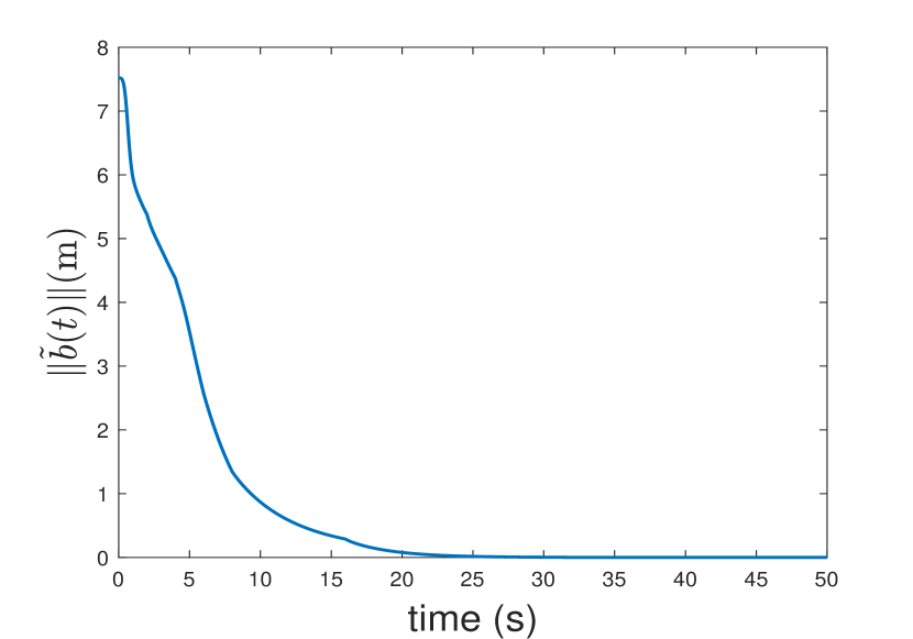
Figure 5: $\|\tilde{b}(t)\|(m)$ vs time ($s$).

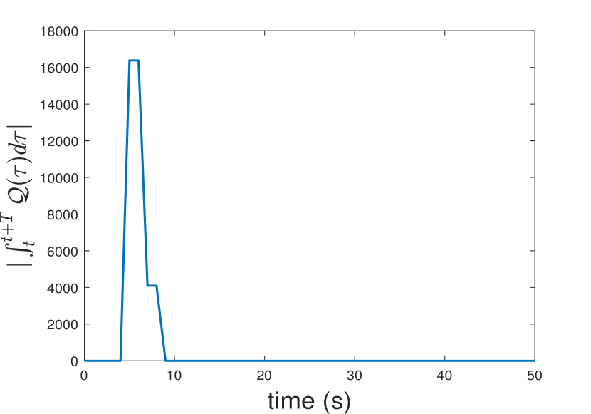
Figure 6: Determinant of $\int_{t}^{t+T}\mathcal{Q}(\tau)\;\textrm{d}\tau$ over time $t$, $T=4s$.

VII Conclusion

In this article we propose a novel distributed adaptive controller to estimate bias in relative position measurements along with guaranteed exact consensus in a network of double-integrator systems. It is shown that joint $(\delta,T)$-connectivity and joint non-Bipartite properties of the graph are necessary for bias estimation and consensus. In future work, we seek to explore more general measurement errors and nonlinear agent dynamics. We will also focus on consensus under erroneous relative measurements over directed and time varying communication graphs.

VIII Acknowledgement

The authors thank Sayan Basu Roy (IIIT Delhi, India), Antonio Loria and Elena Panteley (LSS, CNRS,France), Constantin Morarescu and Vineeth Varma (CRAN, CNRS, France) for their valuable technical inputs.

References

• [1] J. Qin, H. Gao, and W. X. Zheng, “Second-order consensus for multi-agent systems with switching topology and communication delay,” Systems & Control Letters, vol. 60, no. 6, pp. 390–397, 2011.
• [2] Y. Xie and Z. Lin, “Global optimal consensus for multi-agent systems with bounded controls,” Systems & Control Letters, vol. 102, pp. 104–111, 2017.
• [3] X. Wang and Y. Hong, “Finite-time consensus for multi-agent networks with second-order agent dynamics,” IFAC Proceedings volumes, vol. 41, no. 2, pp. 15 185–15 190, 2008.
• [4] Z. Meng, Z. Zhao, and Z. Lin, “On global leader-following consensus of identical linear dynamic systems subject to actuator saturation,” Systems & Control Letters, vol. 62, no. 2, pp. 132–142, 2013.
• [5] Q. Wang and H. Gao, “Global consensus of multiple integrator agents via saturated controls,” Journal of the Franklin Institute, vol. 350, no. 8, pp. 2261–2276, 2013.
• [6] W. Ren and Y. Cao, Distributed Coordination of Multi-agent Networks, 1st ed.   London: Springer-Verlag, 2011, ch. 1,6.
• [7] A. Amirkhani and A. H. Barshooi, “Consensus in multi-agent systems: a review,” Artificial Intelligence Review, pp. 1–39, 2021.
• [8] F. Liu, A. S. Morse, and B. D. Anderson, “Robust control of undirected rigid formations with constant measurement bias in relative positions,” in 2016 American Control Conference (ACC).   IEEE, 2016, pp. 143–147.
• [9] Z. Meng, B. D. Anderson, and S. Hirche, “Formation control with mismatched compasses,” Automatica, vol. 69, pp. 232–241, 2016.
• [10] H. G. De Marina, M. Cao, and B. Jayawardhana, “Controlling rigid formations of mobile agents under inconsistent measurements,” IEEE Transactions on Robotics, vol. 31, no. 1, pp. 31–39, 2014.
• [11] J. Thienel and R. M. Sanner, “A coupled nonlinear spacecraft attitude controller and observer with an unknown constant gyro bias and gyro noise,” IEEE transactions on Automatic Control, vol. 48, no. 11, pp. 2011–2015, 2003.
• [12] J. Boskovic, S.-M. Li, and R. Mehra, “A globally stable scheme for spacecraft control in the presence of sensor bias,” in 2000 IEEE Aerospace Conference. Proceedings (Cat. No. 00TH8484), vol. 3.   IEEE, 2000, pp. 505–511.
• [13] N. Metni, J.-M. Pflimlin, T. Hamel, and P. Soueres, “Attitude and gyro bias estimation for a flying uav,” in 2005 IEEE/RSJ International Conference on Intelligent Robots and Systems.   IEEE, 2005, pp. 1114–1120.
• [14] P. Patre and S. M. Joshi, “Accommodating sensor bias in mrac for state tracking,” AIAA Guidance, Navigation, and Control Conference, 2011.
• [15] G. Troni and L. L. Whitcomb, “Adaptive estimation of measurement bias in three-dimensional field sensors with angular rate sensors: Theory and comparative experimental evaluation.” in Robotics: Science and Systems.   Citeseer, 2013.
• [16] N. Liu, R. Ling, Q. Huang, and Z. Zhu, “Second-order super-twisting sliding mode control for finite-time leader-follower consensus with uncertain nonlinear multiagent systems,” Hindawi Publishing Corporation Mathematical Problems in Engineering, vol. 2015, 2015.
• [17] J. Qin, G. Zhang, W. X. Zheng, and Y. Kang, “Adaptive sliding mode consensus tracking for second-order nonlinear multiagent systems with actuator faults,” IEEE Transactions on Cybernetics, vol. 45, no. 5, pp. 1605 – 1615, May 2019.
• [18] L. Mo, T. Pan, S. Guo, and Y. Niu, “Distributed coordination control of first- and second-order multiagent systems with external disturbances,” Hindawi Publishing Corporation Mathematical Problems in Engineering, vol. 2015, 2015.
• [19] X. Wang and S. Li, “Nonlinear consensus algorithms for second-order multi-agent systems with mismatched disturbances,” 2015 American Control Conference (ACC), pp. 1740–1745, July 2015.
• [20] H. Garcia de Marina, M. Cao, and B. Jayawardhana, “Controlling rigid formations of mobile agents under inconsistent measurements,” IEEE Transactions on Robotics, vol. 31, no. 1, pp. 31–39, 2015.
• [21] K. S. Narendra and A. M. Annaswamy, Stable adaptive systems.   Courier Corporation, 2012.
• [22] S. Boyd and S. Sastry, “On parameter convergence in adaptive control,” Systems & control letters, vol. 3, no. 6, pp. 311–319, 1983.
• [23] M. N. Mahyuddin, G. Herrmann, J. Na, and F. L. Lewis, “Finite-time adaptive distributed control for double integrator leader-agent synchronisation,” in 2012 IEEE international symposium on intelligent control.   IEEE, 2012, pp. 714–720.
• [24] J. Sun and Z. Geng, “Adaptive consensus tracking for linear multi-agent systems with heterogeneous unknown nonlinear dynamics,” International Journal of Robust and Nonlinear Control, vol. 26, no. 1, pp. 154–173, 2016.
• [25] W. Chen, C. Wen, S. Hua, and C. Sun, “Distributed cooperative adaptive identification and control for a group of continuous-time systems with a cooperative pe condition via consensus,” IEEE Transactions on Automatic Control, vol. 59, no. 1, pp. 91–106, 2013.
• [26] H. Dong, Q. Hu, and M. R. Akella, “Composite adaptive control for robot manipulator systems,” 5th CEAS Conference on Guidance, Navigation and Control, 2019.
• [27] S. B. Roy, S. Bhasin, and I. N. Kar, “Composite adaptive control of uncertain euler-lagrange systems with parameter convergence without pe condition,” Asian Journal of Control, vol. 21, no. 6, p. 2137–2149, November 2009.
• [28] T. Garg and S. B. Roy, “Distributed composite adaptive synchronization of multiple uncertain euler-lagrange systems using cooperative initial excitation,” in 2020 59th IEEE Conference on Decision and Control (CDC).   IEEE, 2020, pp. 5816–5821.
• [29] G. Chowdhary, T. Yucelen, M. Mühlegg, and E. N. Johnson, “Concurrent learning adaptive control of linear systems with exponentially convergent bounds,” International Journal of Adaptive Control and Signal Processing, vol. 27, no. 4, pp. 280–301, 2013. [Online]. Available: https://onlinelibrary.wiley.com/doi/abs/10.1002/acs.2297
• [30] S. Djaidja, Q. H. Wu, , and H. Fang, “Leader-following consensus of double-integrator multi-agent systems with noisy measurements,” International Journal of Control, Automation, and Systems, vol. 13, no. 1, pp. 17–24, February 2015.
• [31] D. B. Kingston, W. Ren, and R. W. Beard, “Consensus algorithms are input-to-state stable,” in Proceedings of the 2005, American Control Conference, 2005.   IEEE, 2005, pp. 1686–1690.
• [32] A. Garulli and A. Giannitrapani, “Analysis of consensus protocols with bounded measurement errors,” Systems & Control Letters, vol. 60, no. 1, pp. 44–52, 2011.
• [33] M. Shi, P. Tesi, and C. De Persis, “Self-triggered network coordination over noisy communication channels,” IEEE Transactions on Automatic Control, vol. 65, no. 1, pp. 263–270, 2019.
• [34] D. Tandon and S. Sukumar, “Rigid body consensus under relative measurement bias,” AAS Spaceflight Mechanics meeting, San Antonio, TX, USA, February 2017.
• [35] S. Sukumar, E. Panteley, A. Lorıa, and W. Pasillas, “On consensus of double integrators over directed graphs and with relative measurement bias,” 2018 IEEE Conference on Decision and Control (CDC), 17-19 Dec 2018.
• [36] H. Sinhmar and S. Sukumar, “Distributed model independent algorithm for spacecraft synchronization under relative measurement bias,” 5th CEAS Conference on Guidance, Navigation and Control, 2019.
• [37] M. Shi, C. De Persis, P. Tesi, and N. Monshizadeh, “Bias estimation in sensor networks,” IEEE Transactions on Control of Network Systems, vol. 7, no. 3, pp. 1534–1546, 2020.
• [38] B. D. O. Anderson, G. Shi, and J. Trumpf, “Convergence and state reconstruction of time-varying multi-agent systems from complete observability theory,” IEEE Transactions on Automatic Control, vol. 62, no. 5, pp. 2519–2523, 2017.
• [39] A. S. Asratian, T. M. J. Denley, and R. Häggkvist, Bipartite Graphs and their Applications, ser. Cambridge Tracts in Mathematics.   Cambridge University Press, 1998.
• [40] D. Cvetković, P. Rowlinson, and S. K. Simić, “Signless laplacians of finite graphs,” Linear Algebra and its Applications, vol. 423, no. 1, pp. 155 – 171, 2007, special Issue devoted to papers presented at the Aveiro Workshop on Graph Spectra. [Online]. Available: http://www.sciencedirect.com/science/article/pii/S0024379507000316
• [41] N. R. Chowdhury, S. Sukumar, M. Maghenem, and A. Loría, “On the estimation of the consensus rate of convergence in graphs with persistent interconnections,” International Journal of Control, vol. 91, no. 1, pp. 132–144, 2018. [Online]. Available: https://doi.org/10.1080/00207179.2016.1272006
• [42] S. B. Roy, “Relaxing persistence of excitation for parameter convergence in adaptive control: an initial excitation based approach,” Ph.D. dissertation, Indian Institute of Technology, Delhi, 2019.
• [43] D. S. Bernstein, Matrix Mathematics: Theory, Facts, and Formulas (Second Edition).   Princeton University Press, 2009.
• [44] K. Sridhar and S. Sukumar, “Finite-time, event-triggered tracking control of quadrotors,” in 5th CEAS Specialist Conference on Guidance, Navigation & Control (EurGNC 19) Milano, Italy, April 2019.