Label Efficient Regularization and Propagation for Graph Node Classification

Abstract

An enhanced label propagation (LP) method called GraphHop was proposed recently. It outperforms graph convolutional networks (GCNs) in the semi-supervised node classification task on various networks. Although the performance of GraphHop was explained intuitively with joint node attribute and label signal smoothening, its rigorous mathematical treatment is lacking. In this paper, we propose a label efficient regularization and propagation (LERP) framework for graph node classification, and present an alternate optimization procedure for its solution. Furthermore, we show that GraphHop only offers an approximate solution to this framework and has two drawbacks. First, it includes all nodes in the classifier training without taking the reliability of pseudo-labeled nodes into account in the label update step. Second, it provides a rough approximation to the optimum of a subproblem in the label aggregation step. Based on the LERP framework, we propose a new method, named the LERP method, to solve these two shortcomings. LERP determines reliable pseudo-labels adaptively during the alternate optimization and provides a better approximation to the optimum with computational efficiency. Theoretical convergence of LERP is guaranteed. Extensive experiments are conducted to demonstrate the effectiveness and efficiency of LERP. That is, LERP outperforms all benchmarking methods, including GraphHop, consistently on five test datasets and an object recognition task at extremely low label rates (i.e., 1, 2, 4, 8, 16, and 20 labeled samples per class).

1 Introduction

Semi-supervised learning that exploits both labeled and unlabeled data in learning tasks is highly in demand in real-world applications due to the expensive cost of data labeling and the availability of a large number of unlabeled samples. For graph problems where very few labels are available, the geometric or manifold structure of unlabeled data can be leveraged to improve the performance of classification, regression, and clustering algorithms. Graph convolutional networks (GCNs) have been accepted by many as the de facto tool in addressing graph semi-supervised learning problems [1, 2, 3, 4]. Simply speaking, based on the input feature space, each layer of GCNs applies transformation and propagation through the graph and nonlinear activation to node embeddings. The GCN parameters are learned via label supervision through backpropagation [5]. The joint attributes encoding and propagation as smoothening regularization enables GCNs to produce a prominent performance on various real-world networks.

There are, however, remaining challenges in GCN-based semi-supervised learning. First, GCNs require a sufficient number of labeled samples for training. Instead of deriving the label embeddings from the graph regularization as traditional methods do [6, 7], GCNs need to learn a series of projections from the input feature space to the label space. These embedding transformations largely depend on ample labeled samples for supervision. Besides, nonlinear activation prevents GCNs from provable convergence. The lack of sufficient labeled samples may make training unstable (or even divergent). To improve it, one may integrate other semi-supervised learning techniques (e.g., self- and co-training [8]) with GCN training or enhance the filter power to strengthen the regularization effect [9]. They are nevertheless restricted by internal deficiencies of GCNs. Second, GCNs usually consist of two convolutional layers and, as a result, the information from a small neighborhood for each node is exploited [1, 10, 2, 11]. The learning ability is handicapped by ignoring correlations from nodes of longer distances. Although increasing the number of layers could be a remedy, this often leads to an oversmoothening problem and results in inseparable node representations [8, 12]. Furthermore, a deeper model needs to train more parameters which requires even more labeled samples.

Inspired by the traditional PageRank [13] and label propagation (LP) algorithms [6, 7], some work discards feature transformations at every layer but maintains a few with additional embedding propagation [14, 15, 16, 17]. This augments regularization strength by capturing longer distance relationships and reduces the number of training parameters for label efficiency. Nonetheless, labels still serve as the guidance to model parameters training rather than direct supervision in the label embedding space. As a result, the methods still suffer the unstable training problem and lack of supervision at very low label rates. Along with this research idea, the C&S method [16] applied the optimization procedure to the label space directly with the same propagation as given in [7]. Yet, it was originally designed for supervised learning, and its performance deteriorates significantly if the number of labeled samples decreases. Also, a simple propagation strategy in Laplacian learning may suffer from the degeneracy issue; namely, the solution is localized as spikes near the labeled samples and almost constant far from them [18, 19, 20]. This is caused by a naive propagation procedure where the information cannot be carried over longer distances.

An enhancement of traditional label propagation, called GraphHop, was recently proposed in [21]. GraphHop achieves state-of-the-art performance as compared with GCN-based methods [1, 8, 10] and other classical propagation-based algorithms [7, 22, 23]. It performs particularly well at extremely low label rates. Unlike GCNs that integrate node attributes and smoothening regularization into one end-to-end training system, GraphHop adopts a two-stage learning mechanism. Its initialization stage extracts smoothened node attributes and exploit them to predict label distributions of each node through logistic regression (LR) classifiers. The predicted label embeddings can be viewed as signals on graphs, and additional smoothening steps are applied in the subsequent iteration stage consisting of two steps: 1) label aggregation and 2) label update. In the first step, label embeddings of local neighbors are aggregated, corresponding to low-pass filtering in the label space. To address ineffective propagation in extremely low label rates, LR classifiers are used in the second step for parameter sharing. These two steps are conducted sequentially in each iteration for label signal smoothening. Although the superior performance of GraphHop was explained from the signal processing viewpoint (e.g., low-pass filtering on both attribute and label signals) in [21], its mathematical treatment was not rigorous.

In this work, we first analyze the superior performance of GraphHop from a variational viewpoint, which is mathematically rigorous and transparent. To achieve this, we present a certain optimization problem with probability constraints under the regularization framework. In addition, we propose an alternate optimization strategy for solutions, leading to an optimization of two non-convex subproblems. In the meantime, we show the connection that the two steps (i.e., label aggregation and label update) in the iteration stage of GraphHop can be interpreted as an optimization process for these two subproblems under convex transformation.

Based on this variational interpretation, we point out two drawbacks of GraphHop. First, the LR classifiers adopt all pseudo-labels into training in the label update step, which usually suffers from the wrong predictions. Second, only one aggregation of label embeddings is performed in the label aggregation step, which is a rough approximation to the optimum. We propose a new method called “label efficient regularization and propagation (LERP)” to address these two shortcomings. First, LERP determines reliable pseudo-labeled nodes adaptively based on the distance to the labeled nodes in each alternate round. Second, label embeddings in LERP are propagated in several iterations for a better and efficient approximation to the solution.

The main contributions of this work are summarized below.

1. A label efficient regularization and propagation framework with its alternate optimization solution are proposed. Additionally, we show that GraphHop can be analogized to this alternate procedure with convex transformation to the subproblems.

2. Based on the theoretical understanding, we point out two drawbacks in GraphHop and further propose two corresponding enhancements, which lead to an even more powerful semi-supervised solution called LERP. A mathematical proof of its convergence is given.

3. We demonstrate the effectiveness and efficiency of LERP with extensive experiments on five commonly used datasets as well as an object recognition task at extremely low label rates (i.e., 1, 2, 4, 8, 16 and 20 labeled samples per class).

The rest of this paper is organized as follows. The problem definition and some background information are stated in Sec. 2. A label efficient regularization and propagation framework is set up and its connection with GraphHop is built in Sec. 3. The LERP method is presented in Sec. 4. Theoretical analysis of the convergence and computational complexity are analyzed in Sec. 5. Extensive experiments are conducted for performance benchmarking in Sec. 6. Comments on related work are provided in Sec. 7. Finally, concluding remarks are given in Sec. 8.

2 Preliminaries

2.1 Notations and Problem Statement

To begin with, we define some notations used throughout this paper and give the definition to the investigated problem. An undirected graph is given by $\mathcal{G}=(\mathcal{V},\mathcal{E})$, where $\mathcal{V}$ is the node set with $|\mathcal{V}|=n$ and $\mathcal{E}$ is the edge set. The graph structure can be described by adjacency matrix $\mathbf{A}\in\mathbb{R}^{n\times n}$, where $\mathbf{A}_{ij}=1$ if node $i$ and $j$ are linked by an edge in $\mathcal{G}$. Otherwise, $\mathbf{A}_{ij}=0$. For $\mathbf{A}$, its diagonal degree matrix is $\mathbf{D}_{ii}=\sum_{j=1}^{n}\mathbf{A}_{ij}$ and its graph Laplacian matrix is $\mathbf{L}=\mathbf{D}-\mathbf{A}$. In an attributed graph, each node is associated with a $d$-dimensional feature vector $\mathbf{x}_{i}\in\mathbb{R}^{d}$, where the feature space of all nodes is $\mathbf{X}\in\mathbb{R}^{n\times d}$.

In a transductive semi-supervised classification problem, nodes in set $\mathcal{V}$ can be divided into sets of labeled nodes $\mathcal{L}$ with $l$ samples and unlabeled nodes $\mathcal{U}$ with $u$ samples followed by $n=l+u$. Let $\mathbf{Y}=(\mathbf{y}_{1}^{T},\cdots,\mathbf{y}_{l}^{T},\mathbf{y}_{l+1}^{T},\cdots,\mathbf{y}_{n}^{T})^{T}\in\mathbb{R}^{n\times c}$ denote the given labels of all samples, where $\mathbf{y}_{i}\in\mathbb{R}^{c}$ is a row vector and $c$ is the number of classes. If labeled node $i$ belongs to class $j$, $\mathbf{y}_{ij}=1$; otherwise, $\mathbf{y}_{ij}=0$. To record the predicted label distribution of each node, the label embedding matrix is defined as $\mathbf{F}=(\mathbf{f}_{1}^{T},\cdots,\mathbf{f}_{l}^{T},\mathbf{f}_{l+1}^{T},\cdots,\mathbf{f}_{n}^{T})^{T}\in\mathbb{R}^{n\times c}$ with probability entries, where the $i$th row vector satisfying $\sum_{j=1}^{c}\mathbf{f}_{ij}=1$ with $\mathbf{f}_{ij}$ is the probability of node $i$ belonging to class $j$. The classes of unlabeled nodes can be assigned as $y_{i}=\arg\max_{1\leq j\leq c}\mathbf{f}_{ij}$. Given graph $\mathcal{G}$, node attributes $\mathbf{X}$, and labeled samples $\mathbf{Y}$, the objective is to infer labels of unlabeled nodes under the condition $l\ll u$.

2.2 Transductive Label Propagation

We introduce the general regularization framework for transductive LP algorithms below. Formally, it can be defined as a problem that minimizes the objective function:

$$\min_{\mathbf{F}}\quad\text{tr}(\mathbf{F}^{T}\mathbf{\tilde{L}}\mathbf{F})+\text{tr}((\mathbf{F}-\mathbf{Y})^{T}\mathbf{U}(\mathbf{F}-\mathbf{Y})),$$ (1)

where $\text{tr}(\cdot)$ is the trace operator, $\mathbf{\tilde{L}}$ is the random-walk (or symmetric) normalized graph Laplacian matrix, and $\mathbf{U}=\text{diag}(u_{1},\cdots,u_{n})$ is a positive weighting matrix that balances the manifold smoothness and label fitness. For generality, we relax the probability constraints on label embeddings $\mathbf{F}$.

The closed-form solution of Eq. (1) can be derived as

$$\mathbf{F}^{*}=(\mathbf{U}+\mathbf{\tilde{L}})^{-1}\mathbf{U}\mathbf{Y}.$$ (2)

This result can also be obtained from an iteration process named LP. At each iteration, the label embedding information of each node is partially propagated by its neighbors and partially obtained from its given label. Formally, at iteration $t$, the propagation can be described as

$$\mathbf{F}^{(t)}=\alpha\mathbf{\tilde{A}}\mathbf{F}^{(t-1)}+(1-\alpha)\mathbf{Y},$$ (3)

where $\alpha\in(0,1)$ is a weighting hyperparameter and $\mathbf{\tilde{A}}$ is the random-walk (or symmetric) normalized adjacency matrix. The converged label embedding matrix can be obtained by taking the limit of iterations as

$$\mathbf{F}^{*}=(1-\alpha)(\mathbf{I}-\alpha\mathbf{\tilde{A}})^{-1}\mathbf{Y},$$ (4)

which is the same as Eq. (2) by setting

$$\mathbf{U}=\text{diag}(\frac{1-\alpha}{\alpha},\cdots,\frac{1-\alpha}{\alpha}).$$

2.3 GraphHop

The recently proposed GraphHop model improves traditional LP methods and offers state-of-the-art performance on several datasets. There are two training stages in GraphHop (i.e., the initialization stage and the iteration stage). They are used to capture the smooth node attributes and label embeddings, respectively, as explained below.

In the initialization stage, smoothened attribute signals are extracted by aggregating the neighborhood of each node. Formally, this can be expressed as

$$\mathbf{X}_{M}=||_{0\leq m\leq M}\mathbf{\tilde{A}}^{m}\mathbf{X},$$ (5)

where $||$ denotes column-wise concatenation, $\mathbf{\tilde{A}}^{m}$ is the random-walk normalized $m$-hop adjacency matrix ($m=0$ indicates the attribute of each node itself), and $\mathbf{X}_{M}\in\mathbb{R}^{n\times d(M+1)}$ is the smoothened attribute matrix. After that, a logistic regression (LR) classifier is adopted for training with labeled samples as supervision. The minimization of cross-entropy loss can be written as

$$\min_{\mathbf{W}}\quad-\frac{1}{l}\sum_{i=1}^{l}\mathbf{y}_{i}\log\left(\sigma(\mathbf{W}\mathbf{x}_{M,i}^{T})\right),$$ (6)

where $\mathbf{x}_{M,i}$ is the $i$th row of $\mathbf{X}_{M}$, $\mathbf{W}\in\mathbb{R}^{c\times d(M+1)}$ is the parameter matrix and $\sigma(\mathbf{z})_{i}=e^{z_{i}}\big{/}\sum_{j=1}^{c}e^{z_{j}}$ is the softmax function. The solution to Eq. (6) can be derived by any optimization algorithm (e.g., stochastic gradient descent). Once the classifier converges, the label embeddings of all nodes can be predicted. They serve as the initial embeddings to the subsequent iteration stage. Formally, this can be written as

$$\mathbf{F}^{(0)}=\mathbf{F}_{init}=\sigma(\mathbf{X}_{M}\mathbf{W}^{T}),$$ (7)

where the softmax function, $\sigma(\mathbf{z})$, is applied in a row-wise fashion. Note that in the original GraphHop model, distinct classifiers are trained independently w.r.t. different hops of aggregations, and the final results are the average of all predictions. For simplicity, we only consider one classifier in the variational derivation. The same applies to the iteration stage.

In the iteration stage, there are two steps, called label aggregation and label update, used for label embeddings propagation. In the label aggregation step, the same aggregation as given in Eq. (5) is conducted on label embeddings. Formally, at iteration $t$, we have

$$\mathbf{F}^{(t-1)}_{M}=||_{0\leq m\leq M}\mathbf{\tilde{A}}^{m}\mathbf{F}^{(t-1)},$$ (8)

where $\mathbf{F}_{M}^{(t-1)}\in\mathbb{R}^{n\times c(M+1)}$ is the aggregated nodes’ neighborhood embeddings. In the aggregation of Eq. (8), the embedding parameters are not shared between nodes, i.e., each label embedding is independently derived from their neighborhoods. This will lead to deficient information passing and deteriorate the performance, especially at low label rates. In the label update step, GraphHop trains an LR classifier on the aggregated embedding space and uses inferred label embeddings at the next iteration to overcome the shortcoming mentioned above. The minimization problem of the LR classifier can be stated as

$$\min_{\mathbf{W}}\quad- \sum_{i=1}^{l}\mathbf{y}_{i}\log\left(\sigma(\mathbf{W}\mathbf{f}_{M,i}^{(t-1)^{T}})\right)$$ (9)

$$-\alpha\sum_{i=l+1}^{n}\text{Sharpen}(\mathbf{f}_{i}^{(t-1)})\log\left(\sigma(\mathbf{W}\mathbf{f}_{M,i}^{(t-1)^{T}})\right),$$

where $\mathbf{f}_{M,i}^{(t-1)}$ (resp. $\mathbf{f}_{i}^{(t-1)}$) is the $i$th row of $\mathbf{F}_{M}^{(t-1)}$ (resp. $\mathbf{F}^{(t-1)}$), $\mathbf{W}\in\mathbb{R}^{c\times c(M+1)}$ is the parameter matrix, $\alpha$ is a weighting hyperparameter, and

$$\text{Sharpen}(\mathbf{z})_{i}=z_{i}^{\frac{1}{T}}\big{/}\sum_{j=1}^{c}z_{j}^{\frac{1}{T}}$$

is the sharpening function to control the confidence of the current label embedding distributions. The first term in the objective function is contributed by labeled samples, while the second term is from unlabeled samples, which are pseudo-labels generated by the classifier. Note that we can view the classifier training as a smoothening operation on label signals by sharing the same classifier parameters. Once Eq. (9) has been solved, the inferred label embeddings at iteration $t$ are

$$\mathbf{F}^{(t)}=\sigma(\mathbf{F}_{M}^{(t-1)}\mathbf{W}^{T}).$$ (10)

They serve as the input to the next iteration through Eq. (8). In the entire process of GraphHop, each label embedding is a probability vector.

In summary, the smoothened attributes on graphs are extracted and used for label distribution prediction in the initialization stage. These label embeddings are further smoothened by aggregation and classifier training in the iteration stage and used for final inference.

3 Connection between GraphHop and LERP Framework

The superior performance of GraphHop was explained by joint smoothening of node attributes and label embeddings through propagation and classifier training in the last section. Here, we interpret the smoothening process in GraphHop using a regularization framework, show that it corresponds to an alternate optimization process of a certain objective function with probability constraints.

3.1 Proposed Label Efficient Regularization and Propagation (LERP) Framework

The initialization and iteration stages of GraphHop actually share a similar procedure. The main iterative process arises in the iteration stage. In this subsection, we will derive a variational interpretation for such an iterative process. To begin with, we set up a constrained optimization problem, i.e., the LERP framework:

$$\begin{aligned} \min_{\mathbf{F},\mathbf{W}}\quad&\text{tr}(\mathbf{F}^{T}\mathbf{\tilde{L}}\mathbf{F})+\text{tr}\left((\mathbf{F}-\mathbf{F}_{init})^{T}\mathbf{U}(\mathbf{F}-\mathbf{F}_{init})\right)\\ &+\text{tr}\left((\mathbf{F}-\sigma(\mathbf{F}_{M}\mathbf{W}^{T}))^{T}\mathbf{U}_{\alpha}(\mathbf{F}-\sigma(\mathbf{F}_{M}\mathbf{W}^{T}))\right)\end{aligned}$$ (11)

$$\text{s.t.}\quad\mathbf{F}_{M}=||_{0\leq m\leq M}\mathbf{\tilde{A}}^{m}\mathbf{F},\quad\mathbf{F}\mathbf{1}_{c}=\mathbf{1}_{n},\quad\mathbf{F}\geq\mathbf{0}$$

where $\mathbf{\tilde{L}}=\mathbf{D}^{-1}\mathbf{L}$ is the random-walk normalized graph Laplacian matrix, $\mathbf{F}_{init}$ is the initialized label embeddings from Eq. (7), $\sigma(\mathbf{z})$ is the softmax function applied row-wisely, $\mathbf{U}\in\mathbb{R}^{n\times n}$ and $\mathbf{U}_{\alpha}\in\mathbb{R}^{n\times n}$ are diagonal hyperparameter matrix with positive entries, $\mathbf{1}_{c}\in\mathbb{R}^{c}$ and $\mathbf{1}_{n}\in\mathbb{R}^{n}$ are column vectors of ones, and $\mathbf{W}\in\mathbb{R}^{c\times c(M+1)}$ is the parameter matrix. The last two constraints make each label embedding a probability vector. The cost function in Eq. (11) consists of three terms. The first two give the objective function of the general regularization framework in Eq. (1). The third term is the Frobenius norm on $\mathbf{F}-\sigma(\mathbf{F}_{M}\mathbf{W}^{T})$ if $\mathbf{U}_{\alpha}$ is the identity matrix. It can be viewed as further regularization. The functionality of this extra regularization term can be seen as forcing the label embeddings to be close to the classifier predictions based on neighborhood representations. Thus, the embedding information around labeled nodes can be effectively passed farther distances to unlabeled nodes by sharing a similar neighborhood. This enables the LERP method to have superior performance in extremely low label rates as discussed later in the optimization process. Note that we have replaced the matrix $\mathbf{Y}$ with the initialized label embeddings, $\mathbf{F}_{init}$, derived from Eq. (7) in the cost function.

3.2 Alternate Optimization

We present the optimization procedure for the solution of Eq. (11) and discuss its relationship with GraphHop. Due to the introduction of variable $\mathbf{W}$ in the extra regularization term, the optimization of two variables, $\mathbf{F}$ and $\mathbf{W}$, depends on each other. The problem cannot be solved directly but alternately. We propose an alternate optimization strategy that updates one variable at a time. This alternate optimization strategy has two subproblems. Each of them is a non-convex optimization problem. With approximation and convex transformation, we show that they correspond to the label aggregation and the label update steps in the iteration stage of GraphHop, respectively.

3.2.1 Updating $\mathbf{W}$ with Fixed $\mathbf{F}$

The classifier parameters, $\mathbf{W}$, only exist in the extra regularization term of Eq. (11). Thus, the optimization problem is

$$\min_{\mathbf{W}}\quad\text{tr}\left((\mathbf{F}-\sigma(\mathbf{F}_{M}\mathbf{W}^{T}))^{T}\mathbf{U}_{\alpha}(\mathbf{F}-\sigma(\mathbf{F}_{M}\mathbf{W}^{T}))\right).$$ (12)

By setting $\mathbf{U}_{\alpha}=\text{diag}(u_{\alpha,1},\cdots,u_{\alpha,n})$, Eq. (12) can be written as

$$\min_{\mathbf{W}}\quad\sum_{i=1}^{n}u_{\alpha,i}||\mathbf{f}_{i}^{T}-\sigma(\mathbf{W}\mathbf{f}_{M,i}^{T})||_{2}^{2},$$ (13)

which is a weighted sum of the squared $l_{2}$-norm on the difference between each label embedding and the classifier prediction. It is a non-convex problem due to the softmax function. To address it, we consider the following transformation. Since $\mathbf{f}_{i}$ and $\sigma(\mathbf{W}\mathbf{f}_{M,i}^{T})$ are both probability vectors, it is more appropriate to use the KL-divergence to measure their distance. Then, by converting the $l_{2}$-norm to the KL-divergence and only considering the term w.r.t. parameter $\mathbf{W}$, we are led to the cross-entropy loss minimization:

$$\min_{\mathbf{W}}\quad-\sum_{i=1}^{n}u_{\alpha,i}\mathbf{f}_{i}\log(\sigma(\mathbf{W}\mathbf{f}_{M,i}^{T})).$$ (14)

Note that the optimal solutions to Eq. (13) and Eq. (14) are identical. Besides, we have the following Theorem.

Theorem 1.

The optimization problem in Eq. (14) is a convex optimization problem.

The proof is given in Appendix A.

To further reveal the connection between GraphHop, we rewrite the cost function as contributions from labeled and unlabeled samples in the form of

$$-\sum_{i=1}^{l}u_{\alpha,i}\mathbf{f}_{i}\log(\sigma(\mathbf{W}\mathbf{f}_{M,i}^{T}))-\sum_{i=l+1}^{n}u_{\alpha,i}\mathbf{f}_{i}\log(\sigma(\mathbf{W}\mathbf{f}_{M,i}^{T})).$$ (15)

Instead of adopting the current label embedding (i.e., $\mathbf{f}_{i}$) as supervision for distribution mapping directly, two improvements can be made to the labeled and unlabeled terms, respectively. For the labeled term, we can replace label embeddings with ground-truth labels (i.e., $\mathbf{y}_{i}$) for supervision. For the unlabeled term, since there is no ground-truth label and the current supervision is adopted from the former iteration (i.e., pseudo-labels), a sharpening function can be used to control the confidence of the present pseudo-labels for supervision. Also, by simplifying weighting hyperparameter $u_{\alpha,i}$ to the same value (i.e., $1$ for labeled data and $\alpha$ for unlabeled data), Eq. (15) becomes

$$\min_{\mathbf{W}}\quad- \sum_{i=1}^{l}\mathbf{y}_{i}\log\left(\sigma(\mathbf{W}\mathbf{f}_{M,i}^{T})\right)$$ (16)

$$-\alpha\sum_{i=l+1}^{n}\text{Sharpen}(\mathbf{f}_{i})\log\left(\sigma(\mathbf{W}\mathbf{f}_{M,i}^{T})\right),$$

which is exactly the objective function in the label update step of GraphHop as given by Eq. (9). Eq. (16) is a convex function, and its optimum can be obtained by a standard optimization procedure.

3.2.2 Updating $\mathbf{F}$ with Fixed $\mathbf{W}$

With fixed classifier parameters $\mathbf{W}$, the optimization problem in Eq. (11) becomes

$$\begin{aligned} \min_{\mathbf{F}}\quad&\text{tr}(\mathbf{F}^{T}\mathbf{\tilde{L}}\mathbf{F})+\text{tr}((\mathbf{F}-\mathbf{F}_{init})^{T}\mathbf{U}(\mathbf{F}-\mathbf{F}_{init}))\\ &+\text{tr}\left((\mathbf{F}-\sigma(\mathbf{F}_{M}\mathbf{W}^{T}))^{T}\mathbf{U}_{\alpha}(\mathbf{F}-\sigma(\mathbf{F}_{M}\mathbf{W}^{T}))\right)\end{aligned}$$ (17)

$$\text{s.t.}\quad\mathbf{F}_{M}=||_{0\leq m\leq M}\mathbf{\tilde{A}}^{m}\mathbf{F},\quad\mathbf{F}\mathbf{1}_{c}=\mathbf{1}_{n},\quad\mathbf{F}\geq\mathbf{0}.$$

This is a non-convex optimization problem due to the last regularization term which involves both parameters $\mathbf{F}$ and $\mathbf{F}_{M}$. To solve this, we argue that $\mathbf{F}$ and $\mathbf{F}_{M}$ in the last term should not be optimized simultaneously. The reason is that, in deriving the former subproblem in Eq. (16), the supervision of unlabeled samples are the pseudo-labels from previous iterations. The pseudo-labels should serve as the input (rather than parameters) in the current optimization. For simplicity, we fix the parameter inside $\mathbf{F}_{M}$. Then, we obtain the following optimization problem:

$$\begin{aligned} \min_{\mathbf{F}}\quad&\text{tr}(\mathbf{F}^{T}\mathbf{\tilde{L}}\mathbf{F})+\text{tr}((\mathbf{F}-\mathbf{F}_{init})^{T}\mathbf{U}(\mathbf{F}-\mathbf{F}_{init}))\\ &+\text{tr}\left((\mathbf{F}-\sigma(\mathbf{F}_{M}\mathbf{W}^{T}))^{T}\mathbf{U}_{\alpha}(\mathbf{F}-\sigma(\mathbf{F}_{M}\mathbf{W}^{T}))\right)\end{aligned}$$ (18)

$$\text{s.t.}\quad\mathbf{F}_{M}=||_{0\leq m\leq M}\mathbf{\tilde{A}}^{m}\mathbf{\hat{F}},\quad\mathbf{F}\mathbf{1}_{c}=\mathbf{1}_{n},\quad\mathbf{F}\geq\mathbf{0},$$

where $\mathbf{F}_{M}$ is now a constant derived from the starting label embeddings $\mathbf{\hat{F}}$ of this optimization subproblem. We have the following theorem for this problem.

Theorem 2.

The problem in Eq. (18) is a convex optimization problem.

The proof can be found in Appendix B.1.

A straightforward way to solve this problem is to apply the KKT conditions [24] to the Lagrangian function. Instead, we show a different derivation which is intuitively connected to GraphHop and leading to the same optimum. First, we directly take the derivative of the cost function and set it to zero. It gives

$$\mathbf{F}^{*}=(\mathbf{U}+\mathbf{U}_{\alpha}+\mathbf{\tilde{L}})^{-1}(\mathbf{U}\mathbf{F}_{init}+\mathbf{U}_{\alpha}\sigma(\mathbf{F}_{M}\mathbf{W}^{T})).$$ (19)

Next, we introduce two constants $\mathbf{U}^{\prime}$ and $\mathbf{Y}^{\prime}$:

$$\begin{cases}\begin{aligned} \mathbf{U}^{\prime}&=\mathbf{U}+\mathbf{U}_{\alpha}\\ \mathbf{U}^{\prime}\mathbf{Y}^{\prime}&=\mathbf{U}\mathbf{F}_{init}+\mathbf{U}_{\alpha}\sigma(\mathbf{F}_{M}\mathbf{W}^{T}))\end{aligned}\end{cases}.$$ (20)

By substituting these two terms in Eq. (19), we obtain

$$\mathbf{F}^{*}=(\mathbf{U}^{\prime}+\mathbf{\tilde{L}})^{-1}\mathbf{U}^{\prime}\mathbf{Y}^{\prime}.$$ (21)

It has the same form as Eq. (2). Thus, the same result can be derived from the label propagation process as given in Eq. (3). It can be expressed as

$$\leavevmode\resizebox{465.06001pt}{}{$\begin{aligned} \mathbf{F}^{(t)}&=\mathbf{U}_{\beta}\mathbf{\tilde{A}}\mathbf{F}^{(t-1)}+(\mathbf{I}-\mathbf{U}_{\beta})\mathbf{Y}^{\prime}\\ &\begin{aligned} \ =&\ \mathbf{U}_{\beta}\mathbf{\tilde{A}}\mathbf{F}^{(t-1)}+(\mathbf{I}-\mathbf{U}_{\beta})\\ &\times\big{(}(\mathbf{U}+\mathbf{U}_{\alpha})^{-1}\mathbf{U}\mathbf{F}_{init}+(\mathbf{U}+\mathbf{U}_{\alpha})^{-1}\mathbf{U}_{\alpha}\sigma(\mathbf{F}_{M}\mathbf{W}^{T})\big{)}\end{aligned}\end{aligned}$},$$ (22)

where

$$\mathbf{U}_{\beta}=(\mathbf{I}+\mathbf{U}^{\prime})^{-1}=(\mathbf{I}+\mathbf{U}+\mathbf{U}_{\alpha})^{-1}.$$

This is summarized in the following Proposition.

Proposition 1.

The iteration process in Eq. (22) converges to Eq. (21) and further to Eq. (19).

The proof is given in Appendix B.2. Also, we have the following theorem stating the relationships between the convergence result, i.e., Eq. (19), and the optimal solution to the optimization problem in Eq. (18).

Theorem 3.

If the variable, $\mathbf{F}$, is started in a probabilistic way, i.e., $\mathbf{F}^{(0)}\mathbf{1}_{c}=\mathbf{1}_{n}$ and $\mathbf{F}^{(0)}\geq\mathbf{0}$, then the convergence result (i.e., Eq. (19)) of the iteration process in Eq. (22) is the optimal solution to the optimization problem in Eq. (18).

The proof is shown in Appendix B.3.

Note that starting with a probabilistic distribution can be easily achieved. That is, we can directly adopt the result from the former round of optimization and initialize it as $\mathbf{F}_{init}$. Theorem 3 provides an iterative solution to the optimization problem (18). By comparing the iteration process in Eq. (22) with the label aggregation in Eq. (8) and the label update in Eq. (10) of GraphHop, we see that GraphHop only uses the last term of Eq. (22) without iterations, i.e.,

$$\mathbf{F}^{*}\approx\mathbf{F}^{(0)}=\sigma(\mathbf{F}_{M}\mathbf{W}^{T}),\quad\text{where}\ \mathbf{F}_{M}=||_{0\leq m\leq M}\mathbf{\tilde{A}}^{m}\mathbf{\hat{F}}.$$ (23)

This is a rough approximation to the iteration process in Eq. (22), as well as the optimum in Eq. (19). On the one hand, it does not yield the optimal solution to Eq. (18) in general. On the other hand, it still meets the probability constraints. Most importantly, it lowers the cost of optimizing Eq. (18), which makes GraphHop scalable to large-scale networks.

We summarize the main results of this section as follows. GraphHop offers an alternate optimization solution to the variational problem (11). It roughly solves two approximate subproblems alternatively and iteratively. Its classifier training in the label update step is a convex transformation of the optimization problem in Eq. (12). Its label aggregation and update steps as given in Eqs. (8) and (10) yield an approximate solution to the optimization problem in Eq. (18), which itself is an approximated convex transformation of the problem in Eq. (17). Based on this understanding, we propose an enhancement, named LERP, to address the limitations of GraphHop.

4 Proposed LERP Method

The discussion in the last section reveals two drawbacks in GraphHop, which also leads to two ideas to their improvements. They are elaborated in Secs. 4.1 and 4.2, respectively. An overview of the LERP model is shown in Fig. 1. In the left subfigure, its upper part shows labeled nodes from two different classes (in blue and red) and unlabeled nodes (in gray), while its lower part shows label embeddings predicted by the LR classifier. They serve as the initialization for the subsequent alternate optimization process. The right subfigure depicts the alternate optimization process. It consists of two alternate optimization steps: 1) iterations for label embeddings update and 2) classifier training for classifier parameters update. In the right subfigure, nodes in the curriculum set are colored in green. Only the labeled nodes and nodes in the curriculum set are employed in the classifier training step.

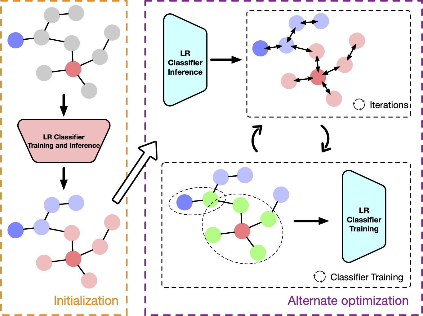
Figure 1: An overview of the LERP method, where the left subfigure shows the initialization for the subsequent process while the right subfigure depicts the alternate optimization process. The latter consists of: 1) iterations for label embeddings update and 2) classifier training for classifier parameters update.

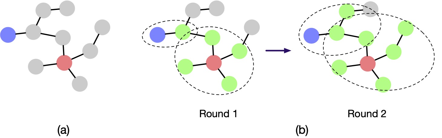
Figure 2: Illustration of growing curriculum sets in the alternate optimization process: (a) the original graph, (b) and (c) selected reliable nodes in the curriculum set in the first and second rounds of the optimization process. Two labeled nodes of two classes are colored in blue and red, unlabeled nodes and nodes in the curriculum set are colored in gray and green, respectively. The dotted ellipses show the corresponding curriculum sets of two labeled nodes.

4.1 Enhancement in Classifier Training

In the subproblem of classifier parameters updating with fixed label embeddings as described in Sec. 3.2.1, the substituted objective function in GraphHop is given in Eq. (16). Unlabeled samples are supervised by label embeddings from the previous iteration, which can be regarded as a self-training process with pseudo-labels. However, the pseudo-labels may not be reliable, which may have a negative impact on classifier training. Besides, this self-training may suffer from label error feedback [25], which makes the classifier biased in the wrong direction. Thus, we should not include all unlabeled samples but the most trustworthy ones in classifier training. Intuitively, the reliability of pseudo-labels of unlabeled samples can be measured by their distances to labeled ones in the network; namely, the closer to labeled samples, the more reliable the pseudo-labels. The rationale is that ground-truth labels should have a stronger influence on their neighborhoods than nodes farther away through propagation.

Formally, we define the collection of reliable nodes as follows.

Definition 1.

The set of reliable nodes is defined by the curriculum set $\mathcal{S}$, which is a subset of unlabeled samples $\mathcal{S}\subseteq\mathcal{U}$. At the $r$th round (starting from $r=1$) of the alternate optimization process, nodes in this set satisfy $\mathcal{S}_{r}=\{u|\min_{v\in\mathcal{V}}\text{dist}(u,v)\leq r,u\in\mathcal{U}\}$, where $\text{dist}(u,v)$ is the shortest path between the two nodes.

In words, at the $r$th round of the optimization process, unlabeled nodes that are within $r$-hop away from the labeled nodes are accepted as reliable nodes and included in the curriculum set. This is illustrated in Fig. 2.

Then, we can modify the objective function of classifier training in Eq. (16) as

$$\min_{\mathbf{W}}\quad- \sum_{i=1}^{l}\mathbf{y}_{i}\log\left(\sigma(\mathbf{W}\mathbf{f}_{M,i}^{T})\right)$$ (24)

$$-\alpha\sum_{i\in\mathcal{S}_{r}}\text{Sharpen}(\mathbf{f}_{i})\log\left(\sigma(\mathbf{W}\mathbf{f}_{M,i}^{T})\right).$$

As a result, only reliable nodes in the curriculum set contribute to classifier training. This enhancement also reduces the training time since there are fewer noisy samples.

4.2 Enhancement in Label Embeddings Update

For the subproblem of label embeddings update with fixed classifier parameters as presented in Sec. 3.2.2, we showed that, starting with a probabilistic distribution of the label embeddings, the optimal solution to Eq. (18) can be derived from an iteration process as given in Eq. (22). For GraphHop, it is further simplified to only the predictions from the classifier without iteration as given in Eq. (23). It is, however, a rough approximation. GraphHop can be enhanced by considering the optimal solution in Eq. (19). Still, the inverse of the Laplacian matrix in Eq. (19) has high time complexity - $\mathcal{O}(n^{3})$, which is not practical. Instead, we adopt the iteration in Eq. (22) to approximate the optimal solution with fewer iterations and avoid matrix inversion. Specifically, we propose the following iteration:

$$\mathbf{F}^{(t)} =\mathbf{U}_{\beta}\mathbf{\tilde{A}}\mathbf{F}^{(t-1)}+(\mathbf{I}-\mathbf{U}_{\beta})\mathbf{F}_{init}$$ (25)

$$=\beta\mathbf{\tilde{A}}\mathbf{F}^{(t-1)}+(1-\beta)\mathbf{F}_{init},$$

where hyperparameters in $\mathbf{U}_{\beta}$ are simplified to be the same $\beta\in(0,1)$ for all nodes. The starting value of the iteration is given by

$$\mathbf{F}^{(0)}=\sigma(\mathbf{F}_{M}\mathbf{W}^{T}),\quad\text{where}\ \mathbf{F}_{M}=||_{0\leq m\leq M}\mathbf{\tilde{A}}^{m}\mathbf{\hat{F}}.$$ (26)

Note that we drop the last classifier inference term $\sigma(\mathbf{F}_{M}\mathbf{W}^{T})$ in Eq. (25) for simplicity since it has already been included in Eq. (26). The balance between $\mathbf{F}_{init}$ and $\sigma(\mathbf{F}_{M}\mathbf{W}^{T})$ can also be achieved by adjusting the weight $\beta$.

If there is no iteration in Eq. (25) (i.e., $t=0$), it degenerates to GraphHop. Another advantage of the iteration is that it can alleviate the oversmoothening problem introduced by continuous label embeddings update in Eq. (23). Since the initial label embeddings $\mathbf{F}_{init}$ are added at each iteration as shown in Eq. (25), the distinct embedding information from the initialization stage is consistently enforced at each node during the optimization process.

With the above two enhancements, the pseudo-codes of LERP are given in Algorithm 1. Note that we adopt the same label initialization as GraphHop as given in Eq. (6), where the enhancements in the alternate optimization are shown in lines 13 to 23. The LR classifier is a linear classifier by nature. Yet, nonlinearity can be introduced with nonlinear kernels. This has not yet been tried in this work.

Algorithm 1 LERP

1:  Input: Graph $\mathbf{A}$, attributes $\mathbf{X}$, label vectors $\mathbf{Y}$

2:  Initialization:

3:  $\mathbf{X}_{M}\leftarrow$ compute Eq. (5)

4:  while not converged do

5:     for each minibatch of labeled nodes do

6:        Compute $\mathbf{g}\leftarrow\nabla{L}(\mathbf{X}_{M},\mathbf{Y};\mathbf{W})$ in Eq. (6)

7:        Conduct Adam update using gradient estimator $\mathbf{g}$

8:     end for

9:  end while

10:  $\mathbf{F}^{(0)}\leftarrow$ compute Eq. (7)

11:  Alternate optimization of Eq. (11):

12:  for $r\in[1,...,max\_round]$ do

13:     for $t\in[1,...,max\_iter]$ do

14:        Compute Eq. (25)

15:     end for

16:     Update the curriculum set $\mathcal{S}$ defined in Definition 1

17:     while not converged do

18:        for each minibatch of all nodes do

19:           Compute $\mathbf{g}\leftarrow\nabla{L}(\mathbf{F},\mathbf{F}_{M},\mathbf{Y};\mathbf{W})$ in Eq. (24)

20:           Conduct Adam update using gradient estimator $\mathbf{g}$

21:        end for

22:     end while

23:     Compute Eq. (26)

24:  end for

25:  Output: Labels of unlabeled nodes $y_{i}=\arg\max_{1\leq j\leq c}\mathbf{f}_{ij}$

5 Theoretical Analysis

In this section, we give the convergence analysis and complexity analysis of the LERP method.

5.1 Convergence Analysis

Theorem 4.

The LERP method monotonically decreases the value of the cost function (11) within a constant difference $2\emph{tr}(\mathbf{U}_{\alpha})$ and with constraints satisfied in each round until the algorithm converges.

The proof is shown in Appendix C.

Theorem 4 indicates that LERP method guarantees the convergence of cost function in problem (11) with all constraints satisfied. Experimental results show that LERP usually converges in less than 20 alternate rounds while the number of iterations of Eq. (25) is less than 10.

5.2 Complexity Analysis

The analysis of time and memory complexities of LERP is similar to [21]. Specifically, we consider one minibatch of nodes since every step in Algorithm 1 can be exercised accordingly. Assume that, during optimization, the number of minibatches is $N$, the number of nodes is $n$, the alternate round of optimization is $r$, the number of iterations is $t$, the size of one minibatch is $b$, and the number of classes is $c$. Then, the time complexity of one minibatch during the entire optimization can be computed as $\mathcal{O}\left(r(n||\mathbf{\tilde{A}}^{M}||_{0}+c||\mathbf{\tilde{A}}^{M}||_{0}/N+tc||\mathbf{\tilde{A}}||_{0}/N+tbc^{2})\right)$ where the first and the second term come from the computation of $M$-hop neighbors and the corresponding aggregation of label embeddings in Eq. (26), the third term comes from the iteration in Eq. (25), and the last term derives from the classifier training in Eq. (24). Note that we can eliminate the first term by only considering the one-hop neighbors (i.e., $M=1$).

The memory usage complexity can be expressed as $\mathcal{O}(bc+c^{2})$ which represents one minibatch embedding and the parameters of the classifier. We ignore the storage of the adjacency matrix since it is the same for all algorithms. Note that the memory cost scales linearly in terms of the minibatch size $b$ and is fixed during the entire optimization process.

6 Experiments

We evaluate LERP on the transductive semi-supervised node classification task with multiple real-word graph datasets in Secs. 6.1-6.6. Furthermore, we apply it to an object recognition problem in Sec. 6.7

6.1 Datasets

For performance benchmarking, we consider five widely used graph datasets whose statistics are shown in Table I, including the numbers of nodes, edges, node labels (i.e., classes), and node feature dimensions. Among them, Cora, CiteSeer, and PubMed [26, 27, 1] are three citation networks. Their nodes represent documents, links indicate citations between documents, labels denote document’s categories, and node features are bag-of-words vectors. Amazon Photo [28, 29] is a co-purchase network. Its nodes represent goods items, and links suggest that the two goods items are frequently purchased together. Its labels are product categories, and node features are bag-of-words encoded product reviews. Coauthor CS [29] is a co-authorship graph. Its nodes are authors, which are connected by an edge if they have a co-authored paper. Node features are keywords of authors’ papers, while a node label indicates the author’s most active fields of study.

TABLE I: Benchmark dataset properties and statistics.

Dataset	Nodes	Edges	Classes	Feature Dims
Cora	$2,708$	$5,429$	$7$	$1,433$
CiteSeer	$3,327$	$4,732$	$6$	$3,703$
PubMed	$19,717$	$44,338$	$3$	$500$
Amazon Photo	$7,487$	$119,043$	$8$	$745$
Coauthor CS	$18,333$	$81,894$	$15$	$6,805$

For data splitting, the standard evaluation of semi-supervised node classification is to sample 20 labeled nodes per class as the training set [1, 29]. To demonstrate the label efficiency of LERP, we examine extremely low label rates in the training set. That is, we sample 1, 2, 4, 8, 16, and 20 labeled nodes per class randomly to form the training set. After that, we follow the standard evaluation procedure by using 500 of the remaining samples as the validation set and the rest as the test dataset. We apply the same dataset split rule to all benchmarking methods for a fair comparison.

6.2 Experimental Settings

6.2.1 Benchmarking Methods, Performance Metrics and Experimental Environment

We compare LERP with representative state-of-the-art methods of the following three categories.

1. GCN-based Methods: GCN [1] and GAT [10].

2. Propagation-based Methods: LP [7], APPNP [14], C&S [16], and GraphHop [21].

3. Label-efficient GCN-based Methods: Co-training GCN [8], self-training GCN [8], IGCN [9], GLP [9], and CGPN [30].

We implement GCN and GAT using the PyG library [31] and LP based on its description. For other benchmarking methods, we adopt their released code. All experimental settings are the same as those specified in their original papers. We run each method on the five datasets as described in Sec. 6.1.

All experiments for LERP and benchmarking methods are conducted ten times on each dataset. The mean test accuracy and the standard deviation are used as the evaluation metric. The experimental environment is a machine with an NVIDIA Tesla V100 GPU (32-GB memory), a ten-core Intel Xeon CPU and 50 GB of RAM.

6.2.2 Implementation Details of LERP

We implement LERP in PyTorch by following GraphHop. That is, we train two independent LR classifiers with one- and two-hop neighborhood aggregation. Thus, there are two LR classifiers trained in the label embedding initialization stage and in the alternate optimization process, respectively. For classifier training, we adopt the Adam optimizer with a learning rate of $0.01$ and $5\times 10^{-5}$ weight decay for regularization. Minibatch training is adopted for larger label rates, while full batch training is used for smaller label rates since there may not be enough labeled samples in a minibatch for the latter. The number of training epochs is set to $1000$ with an early stopping criterion to avoid overfitting. It is observed that the above-mentioned hyperparameters have little impact on classifier training in experiments; namely, the classifier converges efficiently for a wide range of hyperparameters.

We set the maximum number of alternate rounds in the alternate optimization process to 100 for all datasets. Since this number is large enough for LERP to converge as observed in the experiments. We perform a grid search based on validation results in the hyperparameter space of $T$, $\alpha$, $\beta$, and $max\_iter$. The temperature, $T$, in the sharpening function is searched from grid $\{0.1,0.5,1,10,100\}$, the weighting parameter $\alpha$ in the classifier objective function is searched from grid $\{0.1,1,10,100\}$, the weighting parameter $\beta$ in the label embedding iteration is searched from grid $\{0.1,0.5,0.9\}$, and the number of iterations $max\_iter$ is searched from grid $\{1,5,10\}$. These hyperparameters are tuned for different label rates and datasets.

TABLE II: Test accuracy for the Cora dataset with extremely low label rates measured by “mean accuracy ($\%$) $\pm$ standard deviation”. The highest mean accuracy is in bold while the second and third ones are underlined.

Cora
# of labels per class	1	2	4	8	16	20
GCN [1]	$40.48\pm 3.62$	$49.70\pm 1.56$	$67.23\pm 1.34$	$73.88\pm 0.75$	$79.66\pm 0.45$	$81.76\pm 0.25$
GAT [10]	$40.12\pm 5.75$	$50.69\pm 2.08$	$68.82\pm 2.00$	$75.08\pm 0.81$	$79.45\pm 0.59$	$81.59\pm 0.44$
LP [7]	$51.34\pm 0.00$	$54.19\pm 0.00$	$60.64\pm 0.00$	$67.57\pm 0.00$	$69.47\pm 0.00$	$71.03\pm 0.00$
APPNP [14]	$60.70\pm 1.26$	$68.49\pm 1.31$	$75.12\pm 0.93$	$79.15\pm 0.53$	$81.17\pm 0.40$	${82.46\pm 0.61}$
C&S [16]	$37.46\pm 14.90$	$33.93\pm 8.61$	$48.93\pm 9.94$	$64.07\pm 2.62$	$73.63\pm 1.14$	$74.90\pm 1.06$
GraphHop [21]	$59.12\pm 3.18$	$59.21\pm 2.66$	$73.22\pm 0.86$	$75.48\pm 0.90$	$79.29\pm 0.46$	$81.05\pm 0.39$
Co-training GCN [8]	$56.58\pm 0.80$	$66.92\pm 0.73$	$71.95\pm 0.65$	$75.56\pm 0.93$	$77.36\pm 0.76$	$80.17\pm 0.97$
Self-training GCN [8]	$39.71\pm 3.42$	$52.32\pm 6.72$	$65.82\pm 4.85$	$75.16\pm 1.90$	$78.14\pm 0.92$	$80.57\pm 0.59$
IGCN [9]	$61.23\pm 1.94$	$63.75\pm 2.59$	$71.43\pm 0.66$	$78.46\pm 0.57$	$80.04\pm 0.50$	$82.51\pm 0.41$
GLP [9]	$55.67\pm 6.79$	$57.71\pm 3.99$	$70.26\pm 2.68$	$76.78\pm 1.17$	$80.38\pm 0.60$	$82.17\pm 0.71$
CGPN [30]	$70.56\pm 0.00$	$66.41\pm 0.00$	$72.71\pm 0.00$	$76.30\pm 0.00$	$75.91\pm 0.00$	$78.14\pm 0.00$
LERP	$\mathbf{72.47\pm 0.50}$	$\mathbf{73.86\pm 0.67}$	$\mathbf{79.15\pm 0.52}$	$\mathbf{80.07\pm 0.22}$	$\mathbf{81.27\pm 0.56}$	$\mathbf{82.65\pm 0.30}$

TABLE III: Test accuracy for the CiteSeer dataset with extremely low label rates measured by “mean accuracy ($\%$) $\pm$ standard deviation”. The highest mean accuracy is in bold while the second and third ones are underlined.

CiteSeer
# of labels per class	1	2	4	8	16	20
GCN [1]	$26.04\pm 1.65$	$34.69\pm 3.25$	$52.02\pm 0.75$	$61.51\pm 0.87$	$68.03\pm 0.36$	$68.67\pm 0.26$
GAT [10]	$26.83\pm 2.32$	$41.95\pm 3.99$	$52.43\pm 0.97$	$62.86\pm 0.91$	$68.23\pm 0.46$	$68.47\pm 0.51$
LP [7]	$20.10\pm 0.00$	$32.72\pm 0.00$	$33.25\pm 0.00$	$42.21\pm 0.00$	$46.58\pm 0.00$	$47.51\pm 0.00$
APPNP [14]	$34.18\pm 1.53$	$47.04\pm 2.64$	$54.55\pm 0.60$	$65.40\pm 0.47$	$69.46\pm 0.48$	$70.32\pm 0.72$
C&S [16]	$25.34\pm 4.88$	$25.47\pm 3.39$	$37.55\pm 3.19$	$46.24\pm 1.41$	$55.68\pm 1.47$	$57.98\pm 1.22$
GraphHop [21]	$48.40\pm 3.08$	$53.27\pm 5.16$	$54.34\pm 1.66$	$60.11\pm 1.60$	$64.99\pm 1.26$	$67.47\pm 0.66$
Co-training GCN [8]	$28.24\pm 0.27$	$36.55\pm 0.99$	$33.77\pm 3.62$	$58.20\pm 1.06$	$64.10\pm 1.69$	$67.79\pm 0.76$
Self-training GCN [8]	$30.45\pm 5.76$	$36.34\pm 8.54$	$43.59\pm 5.91$	$62.50\pm 3.23$	$68.41\pm 0.84$	$69.63\pm 0.31$
IGCN [9]	$29.63\pm 0.45$	$45.19\pm 1.18$	$51.48\pm 1.88$	$64.49\pm 1.03$	$68.97\pm 0.43$	$69.80\pm 0.28$
GLP [9]	$24.10\pm 5.67$	$40.00\pm 5.45$	$49.83\pm 2.36$	$63.54\pm 1.16$	$68.19\pm 0.89$	$69.10\pm 0.37$
CGPN [30]	$51.93\pm 0.00$	$\mathbf{62.31\pm 0.00}$	$50.55\pm 0.00$	$59.63\pm 0.00$	$63.05\pm 0.00$	$62.91\pm 0.00$
LERP	$\mathbf{53.20\pm 0.85}$	${59.66\pm 0.44}$	$\mathbf{61.04\pm 1.24}$	$\mathbf{66.39\pm 0.44}$	$\mathbf{69.62\pm 0.32}$	$\mathbf{70.77\pm 0.47}$

TABLE IV: Test accuracy for the PubMed dataset with extremely low label rates measured by “mean accuracy ($\%$) $\pm$ standard deviation”. The highest mean accuracy is in bold while the second and third ones are underlined.

PubMed
# of labels per class	1	2	4	8	16	20
GCN [1]	$48.11\pm 9.76$	$65.01\pm 2.05$	$70.99\pm 0.35$	$70.57\pm 0.79$	$76.84\pm 0.26$	$77.38\pm 0.20$
GAT [10]	$57.64\pm 5.52$	$70.04\pm 1.14$	$69.79\pm 0.39$	$71.66\pm 0.30$	$75.62\pm 0.35$	$76.46\pm 0.20$
LP [7]	$63.70\pm 0.00$	$67.16\pm 0.00$	$66.37\pm 0.00$	$65.89\pm 0.00$	$68.63\pm 0.00$	$70.55\pm 0.00$
APPNP [14]	${71.05\pm 0.37}$	${71.37\pm 0.35}$	${71.05\pm 0.19}$	$72.73\pm 1.22$	$\mathbf{79.17\pm 0.39}$	$79.22\pm 0.41$
C&S [16]	$46.58\pm 6.26$	$57.41\pm 8.33$	$67.32\pm 2.00$	$71.08\pm 0.99$	$74.25\pm 0.92$	$74.51\pm 0.85$
GraphHop [21]	$67.13\pm 2.51$	$68.82\pm 0.80$	$69.62\pm 0.31$	$71.21\pm 0.58$	$74.98\pm 0.31$	$76.05\pm 0.32$
Co-training GCN [8]	$62.41\pm 0.35$	$68.70\pm 0.31$	$67.27\pm 0.43$	$69.66\pm 0.17$	$76.21\pm 0.23$	$76.93\pm 0.20$
Self-training GCN [8]	$54.06\pm 7.89$	$70.50\pm 2.83$	$67.43\pm 1.39$	$69.40\pm 1.03$	$73.44\pm 1.92$	$76.96\pm 0.85$
IGCN [9]	$70.17\pm 0.11$	$71.62\pm 0.11$	$70.93\pm 0.08$	$\mathbf{73.45\pm 0.41}$	$78.96\pm 0.28$	$79.53\pm 0.15$
GLP [9]	$70.06\pm 0.32$	$71.30\pm 0.41$	$70.66\pm 0.68$	$73.39\pm 0.33$	$77.92\pm 0.32$	$79.13\pm 0.31$
CGPN [30]	$69.22\pm 0.00$	$69.48\pm 0.00$	$68.38\pm 0.00$	$68.97\pm 0.00$	$68.87\pm 0.00$	$69.93\pm 0.00$
LERP	$\mathbf{72.67\pm 1.79}$	$\mathbf{72.00\pm 0.36}$	$\mathbf{71.11\pm 0.19}$	$72.59\pm 0.07$	$77.20\pm 1.45$	$\mathbf{79.71\pm 0.33}$

TABLE V: Test accuracy for the Amazon Photo dataset with extremely low label rates measured by “mean accuracy ($\%$) $\pm$ standard deviation”. The highest mean accuracy is in bold while the second and third ones are underlined.

Amazon Photo
# of labels per class	1	2	4	8	16	20
GCN [1]	$35.61\pm 3.37$	$39.52\pm 10.35$	$69.55\pm 1.37$	$72.53\pm 0.90$	$75.76\pm 1.06$	$78.21\pm 0.55$
GAT [10]	$46.24\pm 0.00$	$67.66\pm 2.52$	$78.78\pm 4.24$	$83.30\pm 1.86$	$83.54\pm 1.47$	$84.78\pm 1.11$
LP [7]	$61.09\pm 0.00$	$72.96\pm 0.00$	$67.79\pm 0.00$	$76.69\pm 0.00$	$81.32\pm 0.00$	$82.62\pm 0.00$
APPNP [14]	$36.72\pm 29.73$	$33.15\pm 32.40$	$50.90\pm 35.43$	$86.63\pm 0.56$	$88.19\pm 0.57$	$87.50\pm 0.60$
C&S [16]	$33.01\pm 18.02$	$36.47\pm 5.19$	$64.45\pm 4.27$	$78.69\pm 2.44$	$84.67\pm 1.18$	$85.39\pm 1.37$
GraphHop [21]	$58.76\pm 4.12$	$70.86\pm 7.51$	$78.30\pm 2.78$	$83.67\pm 1.24$	$87.16\pm 1.55$	$88.88\pm 0.97$
Co-training GCN [8]	$45.97\pm 6.00$	$56.84\pm 5.29$	$70.82\pm 3.44$	$75.94\pm 2.92$	$79.49\pm 1.11$	$81.45\pm 1.05$
Self-training GCN [8]	$20.21\pm 11.28$	$28.65\pm 8.98$	$65.71\pm 4.80$	$72.69\pm 4.61$	$80.56\pm 2.14$	$83.09\pm 0.87$
IGCN [9]	$29.57\pm 7.03$	$28.70\pm 4.06$	$56.51\pm 1.41$	$67.12\pm 3.24$	$72.77\pm 4.10$	$79.61\pm 1.14$
GLP [9]	$9.12\pm 0.00$	$9.25\pm 0.00$	$26.59\pm 4.20$	$35.58\pm 0.26$	$40.49\pm 5.74$	$55.30\pm 6.56$
CGPN [30]	$62.22\pm 0.00$	$64.76\pm 0.00$	$78.35\pm 0.00$	$80.03\pm 0.00$	$78.14\pm 0.00$	$82.16\pm 0.00$
LERP	$\mathbf{67.41\pm 2.00}$	$\mathbf{83.10\pm 1.58}$	$\mathbf{86.10\pm 0.75}$	$\mathbf{89.26\pm 0.36}$	$\mathbf{91.83\pm 0.33}$	$\mathbf{92.06\pm 0.29}$

TABLE VI: Test accuracy for the Coauthor CS dataset with extremely low label rates measured by “mean accuracy ($\%$) $\pm$ standard deviation”. The highest mean accuracy is in bold while the second and third ones are underlined.

Coauthor CS
# of labels per class	1	2	4	8	16	20
GCN [1]	$64.42\pm 2.14$	$74.07\pm 1.09$	$82.62\pm 0.74$	$87.88\pm 0.55$	$89.86\pm 0.15$	$90.19\pm 0.17$
GAT [10]	$72.81\pm 2.01$	$80.76\pm 1.25$	$85.37\pm 0.94$	$88.06\pm 0.61$	$89.83\pm 0.16$	$89.82\pm 0.17$
LP [7]	$52.63\pm 0.00$	$59.34\pm 0.00$	$61.77\pm 0.00$	$68.60\pm 0.00$	$73.50\pm 0.00$	$74.65\pm 0.00$
APPNP [14]	$71.06\pm 17.48$	$86.18\pm 0.56$	${86.57\pm 0.58}$	$89.66\pm 0.30$	$90.65\pm 0.21$	$90.55\pm 0.17$
C&S [16]	$35.63\pm 13.20$	$67.11\pm 3.50$	$78.57\pm 1.22$	$83.92\pm 1.15$	$87.09\pm 0.95$	$87.97\pm 0.56$
GraphHop [21]	$65.03\pm 0.01$	$77.59\pm 3.17$	$83.79\pm 1.13$	$86.69\pm 0.62$	$89.47\pm 0.38$	$89.84\pm 0.00$
Co-training GCN [8]	$75.78\pm 1.00$	$\mathbf{86.94\pm 0.70}$	$87.40\pm 0.78$	$88.81\pm 0.32$	$89.22\pm 0.42$	$89.01\pm 0.55$
Self-training GCN [8]	$69.69\pm 3.27$	$82.79\pm 4.10$	$87.62\pm 1.49$	$88.82\pm 1.00$	$89.53\pm 0.54$	$89.07\pm 0.70$
IGCN [9]	$62.16\pm 2.81$	$59.56\pm 2.91$	$65.82\pm 4.86$	$86.57\pm 0.78$	$87.76\pm 0.74$	$88.10\pm 0.52$
GLP [9]	$43.56\pm 7.06$	$50.74\pm 7.55$	$46.61\pm 9.85$	$76.61\pm 3.39$	$81.75\pm 2.81$	$82.43\pm 3.31$
CGPN [30]	$67.66\pm 0.00$	$64.49\pm 0.00$	$71.00\pm 0.00$	$77.09\pm 0.00$	$78.75\pm 0.00$	$79.71\pm 0.00$
LERP	$\mathbf{82.46\pm 1.28}$	$86.37\pm 0.37$	$\mathbf{88.45\pm 0.35}$	$\mathbf{89.87\pm 0.48}$	$\mathbf{90.69\pm 0.13}$	$\mathbf{90.87\pm 0.06}$

6.3 Performance Evaluation

The performance results on five graph datasets are summarized in Tables II, III, IV, V, and VI, respectively. Each column shows the classification accuracy (%) of LERP and benchmarking methods on test data under a specific label rate. Overall, LERP has the top performance among all comparators in most cases. In particular, for cases with extremely limited labels, LERP outperforms other benchmarking methods by a large margin. This is because graph convolutional networks are difficult to train with a small number of labels. The lack of supervision prevents them from learning the transformation from the input feature space to the label embedding space with nonlinear activation at each layer. Instead, LERP applies regularization to the label embedding space. It is more effective since it relieves the burden of learning the transformation. A small number of labeled nodes also restricts the efficacy of message passing on graphs of GCN-based methods. In general, only two convolutional layers are adopted by GCN-based methods, which means that only messages in the two-hop neighborhood of each labeled node can be supervised. However, the two-hop neighborhood of a limited number of labeled nodes cannot cover the whole network effectively. Consequently, a large number of nodes do not have supervised training from labels, resulting in an inferior performance of all GCN-based methods. Some label-efficient GCN-based methods try to alleviate this problem by exploiting pseudo-labels as supervision (e.g., self-training GCN) or improving message passing capability (e.g., IGCN and CGPN). However, they are still handicapped by deficient message passing in the graph convolutional layers.

Some propagation-based methods (e.g., LERP, APPNP, and GraphHop) achieve better performance in most datasets with low label rates. This is because the messages from labeled nodes can pass a longer distance on graphs through an iterative process. Yet, although LP and C&S are also propagation-based, their performance is poorer since LP fails to encode the rich node attribute information in model learning while C&S was originally designed for supervised learning and lack of labeled samples degrades its performance significantly.

6.4 Convergence Analysis

Since LERP provides an alternate optimization solution to the problem (11), we show the convergence of label embeddings $\mathbf{F}$ and parameters of LR classifiers $\mathbf{W}$ in Figs. 3 and 4, respectively, to demonstrate its convergence behavior. Fig. 3 shows the accuracy change along with the number of alternate rounds of the optimization process. We see that label embeddings converge in all five benchmarking datasets under different label rates. A smaller label rate requires a larger number of alternate rounds. Since classifiers are trained on reliable nodes as defined in Eq. (24), it needs more alternate rounds to train on the entire node set and propagate label embeddings to the whole graph. Furthermore, the convergence speed is relatively fast. The number of alternate rounds is usually less than 20 in most investigated cases, leading to significant training efficiency as discussed later. Fig. 4 depicts the cross-entropy loss curves as a function of the training epoch for the two LR classifiers at a label rate of 20 labels per class. The number of epochs is counted throughout the whole optimization process. As shown in the figure, the curves converge rapidly in several epochs.

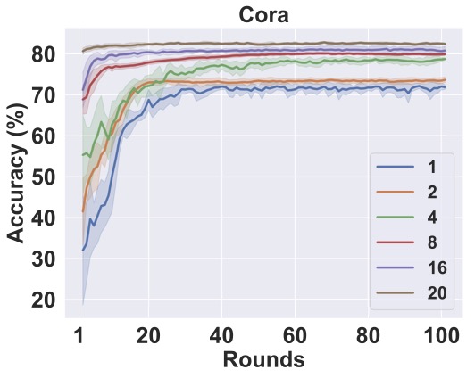
(a)

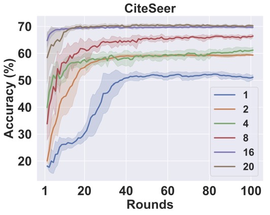
(b)

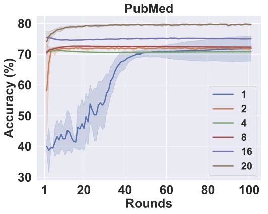
(c)

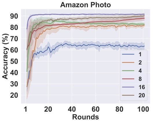
(d)

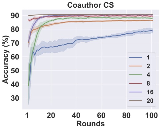
(e)

Figure 3: Convergence results of the label embeddings for the five benchmarking datasets: (a) Cora, (b) CiteSeer, (c) PubMed, (d) Amazon Photo, and (e) Coauthor CS. The $x$-axis is the number of alternate optimization rounds and the $y$-axis is the test accuracy ($\%$). Different curves show the mean accuracy values under different label rates and the shaded areas represent the standard deviation.

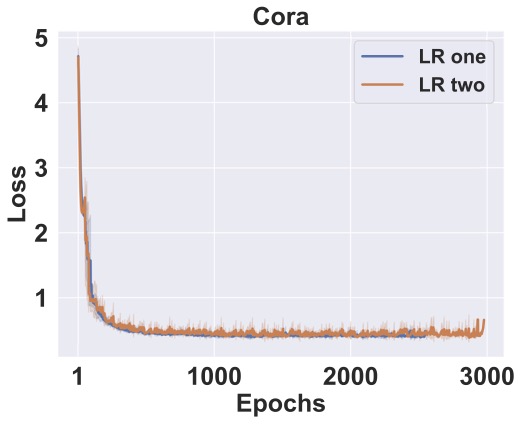
(a)

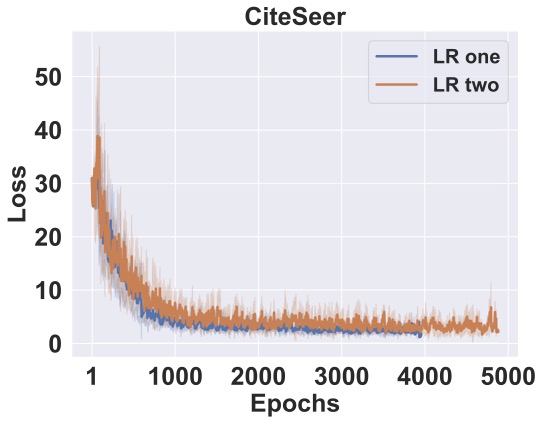
(b)

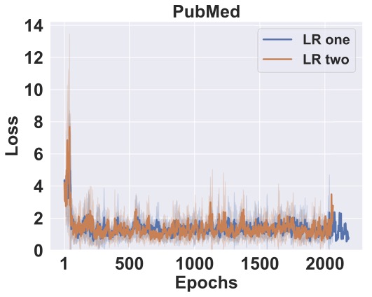
(c)

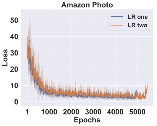
(d)

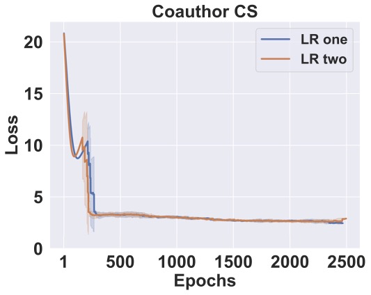
(e)

Figure 4: Convergence results of the LR classifiers for the five benchmarking datasets: (a) Cora, (b) CiteSeer, (c) PubMed, (d) Amazon Photo, and (e) Coauthor CS. The $x$-axis is the number of training epochs and the $y$-axis is the training loss. The label rate is 20 labels per class.

6.5 Complexity and Memory Requirements

We compare the running time performance of LERP and it’s several benchmarking methods. Fig. 5 shows the results at a label rate of 20 labeled samples per class with respect to the five datasets. For LERP, we report results with 100 rounds and 20 rounds, respectively, since it can converge within 20 rounds as indicated in Fig. 3. We see from Fig. 5 that LERP(20) can achieve an average running time. The most time-consuming part of LERP is the training of the LR classifiers, which demands multiple loops of all data samples. However, we find that incorporating classifiers is essential to the superior performance of LERP under limited label rates as discussed later. In other words, LERP trades some time for effectiveness in the case of extremely low label rates. Among all datasets, C&S achieves the lowest running time due to its simple design as LP.

Next, we compare the GPU memory usage of LERP and its several benchmarking methods. The results are shown in Fig. 6, where the values of LERP are taken from the same experiment of running time comparison as given in Fig. 5. Generally, GraphHop and LERP achieve the lowest GPU memory usage among all benchmarking methods against the five datasets. The reason is that GraphHop and LERP allow minibatch training. The only parameters to be stored in the GPU are classifier parameters and one minibatch of data. Instead, the GCN-based methods cannot simply conduct minibatch training. Since embeddings from different layers need to be stored for backpropagation, the GPU memory consumption increases significantly.

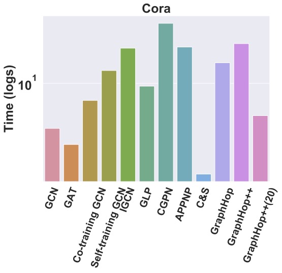
(a)

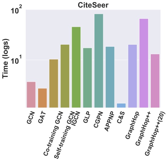
(b)

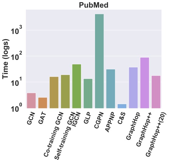
(c)

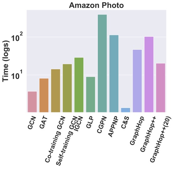
(d)

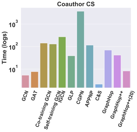
(e)

Figure 5: Comparsion of computational efficiency of different methods measured by log(second) for (a) Cora, (b) CiteSeer, (c) PubMed, (d) Amazon Photo , and (e) Coauthor CS datasets, where the label rate is 20 labeled samples per class and LERP(20) is the result of LERP with 20 alternate optimization rounds.

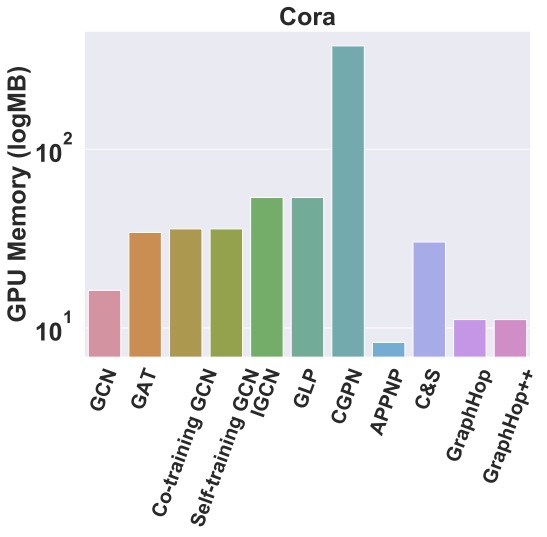
(a)

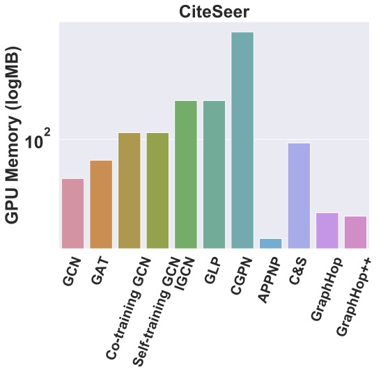
(b)

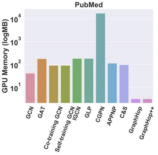
(c)

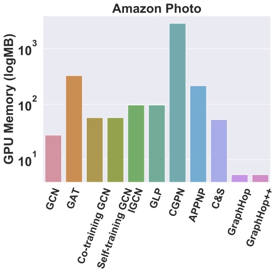
(d)

(e)

Figure 6: Comparsion of of GPU memory usages of different methods measured by log(Mega Bytes) for (a) Cora, (b) CiteSeer, (c) PubMed, (d) Amazon Photo, and (e) Coauthor CS datasets, where the label rate is 20 labeled samples per class.

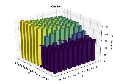
(a)

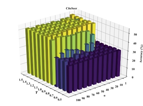
(b)

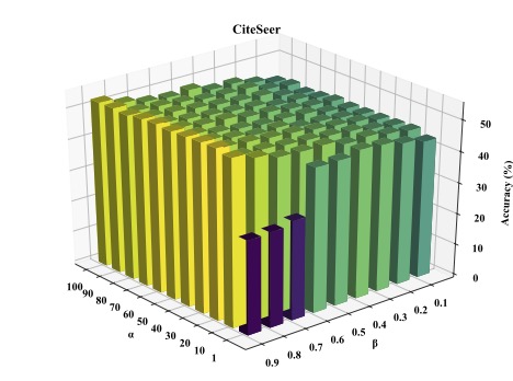
(c)

Figure 7: Performance of LERP with various hyperparameter settings for the CiteSeer dataset, where the $z$-axis is the accuracy result and the label rate is one label per class: (a) performance of $T$ and $\beta$ with fixed $\alpha$, (b) performance of $T$ and $\alpha$ with fixed $\beta$, (c) performance of $\alpha$ and $\beta$ with fixed $T$.

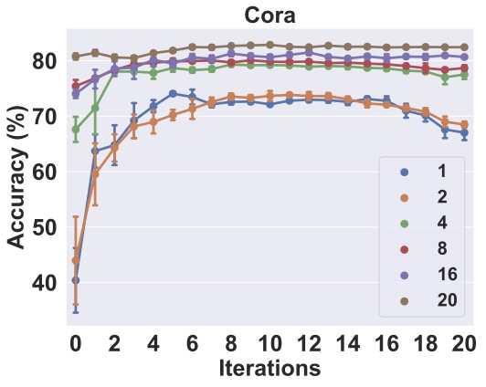
(a)

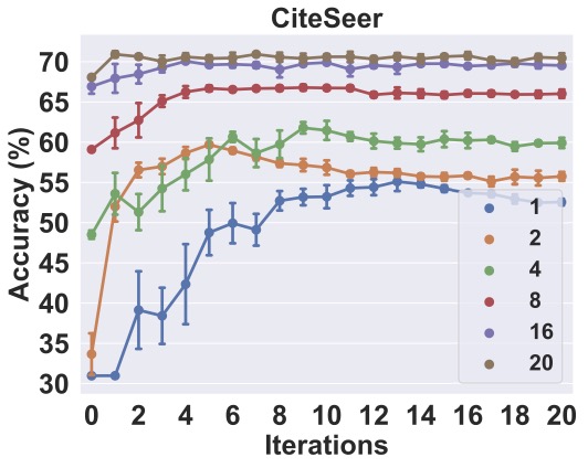
(b)

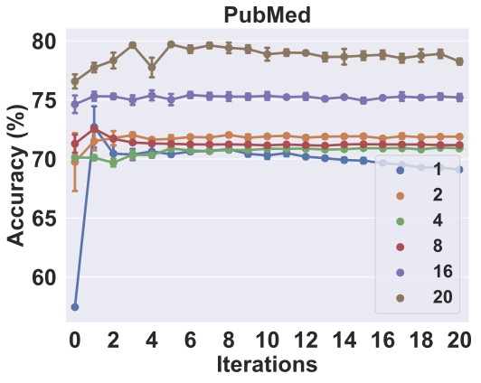
(c)

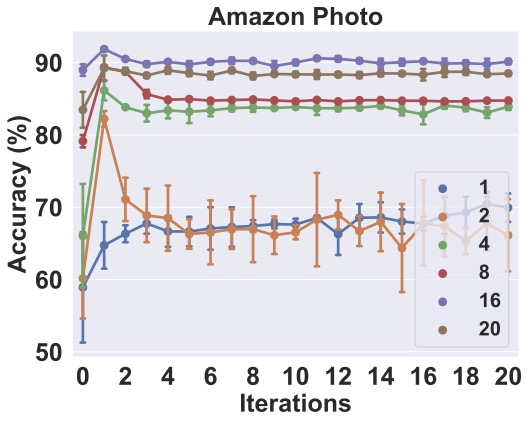
(d)

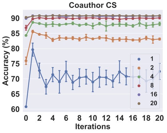
(e)

Figure 8: Performance of LERP with an increasing number of iterations for five datasets: (a) Cora, (b) CiteSeer, (c) PubMed, (d) Amazon Photo, and (e) Coauthor CS, where the $x$-axis is the number of alternate optimization rounds and the $y$-axis is the test accuracy ($\%$). The averaged accuracy under one specific number of iterations is represented as dots and the standard deviation as vertical bars. Different lines denote results under different label rates.

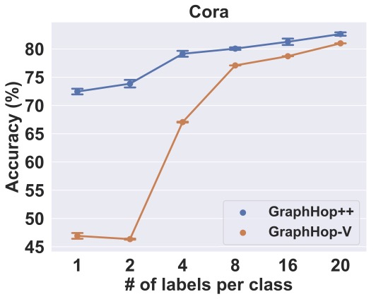
(a)

(b)

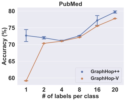
(c)

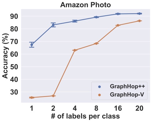
(d)

(e)

Figure 9: Performance comparison of LERP and LERP-V under different label rates: (a) Cora, (b) CiteSeer, (c) PubMed, (d) Amazon Photo, and (e) Coauthor CS datasets.

6.5.1 Parameter Sensitivity

The effects of three hyperparameters, i.e., $T$, $\alpha$ and $\beta$, of LERP on the performance are analyzed here. Due to page limitations, we focus on a representative case in our discussion below, namely, the CiteSeer dataset with a label rate of one-labeled sample per class. To study the effect of three hyperparameters, we fix one and change the other two using grid search. For example, we fix $T$ and adjust $\alpha$ and $\beta$. The sweeping ranges are around the adopted tuning ranges. For each setting, results are averaged over ten runs. They are depicted in Fig. 7.

We have the following observations. First, hyperparameter $T$ has the largest influence on the performance, and a small value will degrade the accuracy result. However, once $T>1$, the performance stays the same. Note that $T=1$ means that there is no sharpening operation on the label distribution in Eq. (16). In practice, we can eliminate hyperparameter $T$ by removing the sharpening operation. Second, $\alpha$ and $\beta$ have less influence on the performance. By increasing $\alpha$ and $\beta$ slightly, the performance improves as shown in Fig. 7. We need to tune these two hyperparameters so as to achieve the best performance.

6.6 Ablation Study

6.6.1 Enhancement via Label Embeddings Update

As compared to GraphHop, LERP has an enhancement by conducting several iterations of label embeddings in Eq. (25). That results in a better approximation to the optimum of Eq. (18). This is experimentally verified below. We measure the accuracy under the same experimental settings but vary the number of iterations, $max\_iter$, from zero to 20. The results against five datasets are shown in Fig. 8. It is worthwhile to point out that LERP degenerates to GraphHop with zero iteration, i.e., only performing Eq. (26). We see from the figure that increasing the number of iterations improves the performance overall. This is especially true when the label rate is very low. Fewer labeled nodes demand a larger number of iterations for better approximation. Furthermore, we observe that the performance improvement saturates within ten iterations. Since several iterations can achieve sufficient approximation with high accuracy, there is no need to reach optimality in label embedding optimization. It saves a considerable amount of running time.

6.6.2 Removing LR Classifier Training

LERP is an alternate approximate optimization of the variational problem given in Eq. (11). If we set hyperparameter $\mathbf{U}_{\alpha}=\mathbf{0}$, the alternate optimization process reduces to label embeddings optimization without the LR classifier training. Note that this is still different from the regularization framework of the classical LP algorithm given in Eq. (1), where the ground-truth label, $\mathbf{Y}$, is changed to the initial label embeddings $\mathbf{F}_{init}$ as supervision. This model without LR classifier training is named “LERP-V (LERP-Variant)”. We conduct experiments of LERP-V on the same five datasets and show the results in Fig. 9. We see that LERP outperforms LERP-V on all datasets under various label rates. The performance gap is especially obvious when the number of labeled samples is very low. This can be explained as follows. Recall that LR classifiers are trained on labeled and reliable nodes and used to infer label embeddings for all nodes in the next round as given in Eq. (26). The inference improves the propagation of label embedding from labeled nodes to the entire graph. This is especially important when label rates are low since the performance of the original propagation as given in Eq. (3) is poor under this situation [20]. Another interesting observation is that this simple variant can achieve performance comparable with that of GCN under the standard setting of 20 labels per class.

6.7 Application to Object Recognition

To show the effectiveness and other potential applications of LERP, we apply it to an object recognition problem in this subsection. COIL20 [32] is a popular dataset for object recognition. It contains 1,440 object images belonging to 20 classes, where each object has 72 images shot from different angles. Some exemplary images are given in Fig. 10. The resolution of each image is $32\times 32$ and each pixel has 256 gray levels. As a result, each image can be represented as a 1024-D vector.

Each image corresponds to a node. A k-nearest neighbor (kNN) graph with $k=7$ is built based on the Euclidean distance of two images; namely, edge weights are the Euclidean distance between two connected nodes. We conduct experiments on this constructed graph for LERP and other benchmarking methods. We tune the hyperparameters of all benchmarks and report the best accuracy performance. As for LERP, we set the number of iterations to 50 and $\alpha=0.99$ for lower label rates. The results under three different label rates are shown in Table VII. LERP achieves the best performance at all three label rates. The high performance of the LP method indicates that the node attribute information (i.e., 1024 image pixels) does not contribute much to label predictions, which is different from other benchmarking datasets. Instead, the manifold regularization of label embeddings is the factor that is most relevant to high performance. This explains the fact that propagation-based methods achieve better accuracy than GCN-based methods at very low label rates. However, once there are enough labeled samples (e.g., 20 labeled samples per class), GCN-based or other propagation-based methods can achieve comparable performance or outperform the LP method. In this case, there are sufficient labeled samples for neural network training. They further exploit the node attribute information in model learning.

TABLE VII: Test accuracy with three label rates measured by “mean accuracy ($\%$) $\pm$ standard deviation”, where the highest mean accuracy is marked in bold and the second and third are underlined.

COIL20
# of labels per class	1	2	20
GCN [1]	$61.05\pm 1.85$	$68.19\pm 3.75$	$88.72\pm 1.64$
GAT [10]	$57.98\pm 5.27$	$65.32\pm 3.36$	$86.66\pm 2.82$
LP [7]	$83.48\pm 0.00$	$85.89\pm 0.00$	$88.89\pm 0.00$
APPNP [14]	$78.11\pm 0.23$	$79.94\pm 0.60$	$90.67\pm 0.45$
C&S [16]	$67.85\pm 4.66$	$75.67\pm 2.79$	$92.50\pm 0.68$
GraphHop [21]	$78.42\pm 2.72$	$78.99\pm 2.95$	$92.70\pm 0.96$
Co-training GCN [8]	$60.07\pm 3.04$	$71.10\pm 2.99$	$91.22\pm 1.12$
Self-training GCN [8]	$59.96\pm 1.95$	$70.32\pm 3.44$	$91.15\pm 0.75$
IGCN [9]	$73.77\pm 4.06$	$75.70\pm 2.46$	$82.24\pm 1.73$
GLP [9]	$45.53\pm 7.44$	$39.79\pm 4.04$	$27.63\pm 3.51$
LERP	$\mathbf{86.75\pm 1.29}$	$\mathbf{87.61\pm 0.27}$	$\mathbf{93.07\pm 1.04}$

7 Related Work

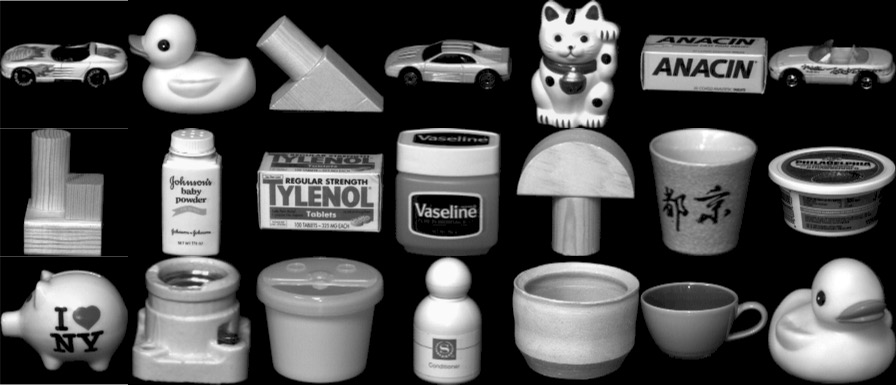
Figure 10: Illustration of several exemplary images of the COIL20 dataset.

GCN-based Methods. Graph convolutional networks (GCNs) have achieved great success in semi-supervised graph learning [1, 2, 10, 33]. Among them, the model proposed by Kipf et al. [1], which adopts the first-order approximation of spectral graph convolution, offered good results in semi-supervised node classification and revealed the identity between the spectral-based graph convolution [34, 35] and the spatial-based message-passing scheme [36, 37]. Afterward, there was an explosion of designs in graph convolutional layers to offer various propagation mechanisms [38, 2, 10, 39]. Numerous applications of graph-structured data arise [40, 39, 41].

However, graph regularization of label distributions in the design of GCNs is not directly connected to label embeddings in model learning, which could undermine the performance. Some work attempts to address this deficiency by proposing a giant graphic model that incorporates label correlations [42, 43, 44]. In practice, these methods are costly with a specific inductive bias and subjective to the local minimum during optimization. Another issue induced is that a sufficient number of labels are required to learn the feature transformation. To improve the label efficiency of GCNs, researchers introduce other semi-supervised learning techniques [8, 45] or improve layer-wise aggregation strength [9, 30]. However, they still inherit deficiencies from graph convolutional layers.

Propagation-based Methods. The propagation-based methods for node classification on graphs can be dated back to the label propagation algorithms in [6, 7]. Recently, there has been a renaissance in combining propagation schemes with advanced neural networks [14, 16, 46, 17, 47]. These methods attempt to encode higher-order correlations but preserve nodes’ local information simultaneously. For example, APPNP [14] propagates neural predictions via label propagation with small contributions of predictions added at each iteration [7]. It gives a superior performance as compared to GCN-based methods. Yet, these methods do not target very low label rates. Besides, the joint learning of feature transformation still requires a considerable amount of labels for training.

8 Conclusion

A label efficient regularization and propagation framework was proposed and a variational interpretation of GraphHop was given in this work. Simply speaking, GraphHop can be viewed as an alternate optimization process that optimizes a regularized function defined by graphs under probability constraints. Based on this understanding, two drawbacks of GraphHop were identified, and a new method called LERP was proposed to address them. LERP solves two convex transformed subproblems in each round with two salient features. First, it determines reliable nodes adaptively for classifier training. Second, it adopts iterations to efficiently offer an improved approximation to the optimal label embeddings. The convergence was guaranteed by the mathematical proof, and the performance of LERP was tested and compared with a large number of existing methods against five commonly used datasets as well as an object recognition problem. Its superior performance, especially at extremely low label rates, demonstrates its effectiveness and efficiency. It would be interesting to apply other regularization schemes to graph learning problems based on the framework of GraphHop and LERP as a future extension.

Appendix A Proof of Theorem 1

Proof.

The cost function in Eq. (14) can be expressed as

$$-\sum_{i=1}^{n}u_{\alpha,i}\sum_{j=1}^{c}f_{ij}\log(\sigma(\mathbf{z})_{j}),$$ (27)

where $\mathbf{z}=\mathbf{W}\mathbf{f}_{M,i}^{T}$ and $\sigma(\mathbf{z})_{j}=e^{z_{j}}\big{/}\sum_{k=1}^{c}e^{z_{k}}$ is the $j$th entry of the vector applied the softmax function. Then, it can be rewritten as

$$\sum_{i=1}^{n}u_{\alpha,i}\sum_{j=1}^{c}f_{ij}\left(\log\big{(}\sum_{k=1}^{c}e^{z_{k}}\big{)}-z_{j}\right).$$ (28)

It is proved in [24] that the log-sum-exp function is a convex function. A nonnegative linear combination of convex functions is still a convex function. Thus, the cost function in Eq. (14) is a convex function, which leads to a convex optimization problem without any constraint. ∎

Appendix B

B.1 Proof of Theorem 2

Proof.

We first prove the cost function in Eq. (18) is a convex function. This is done by showing the second derivative of the cost function is positive semi-definite. Formally, we have

$$\begin{aligned} &\begin{aligned} \nabla^{2}&\bigg{[}\text{tr}(\mathbf{F}^{T}\mathbf{\tilde{L}}\mathbf{F})+\text{tr}((\mathbf{F}-\mathbf{F}_{init})^{T}\mathbf{U}(\mathbf{F}-\mathbf{F}_{init}))\\ &+\text{tr}\left((\mathbf{F}-\sigma(\mathbf{F}_{M}\mathbf{W}^{T}))^{T}\mathbf{U}_{\alpha}(\mathbf{F}-\sigma(\mathbf{F}_{M}\mathbf{W}^{T}))\right)\bigg{]}\end{aligned}\\ &=\mathbf{\tilde{L}}+\mathbf{U}+\mathbf{U}_{\alpha}\end{aligned}.$$ (29)

The first term, $\mathbf{\tilde{L}}$, is the random-walk normalized Laplacian matrix with eigenvalues in the range $[0,2]$. The second and the third terms are both diagonal matrix with positive entries. Therefore, their sum, i.e., the second derivative of the cost function, is positive semi-definite. Besides, since the equality constraint is a linear function and inequality constraint is convex, the domain of the cost function is also convex. So based on the second-order characterization, Eq. (18) is a convex optimization problem. ∎

B.2 Proof of Proposition 1

Proof.

Without loss of generality, we set $\mathbf{F}^{(0)}=\mathbf{F}_{init}$. By Equation (22), we have

$$\mathbf{F}^{(t)}=(\mathbf{U}_{\beta}\mathbf{\tilde{A}})^{t-1}\mathbf{F}_{init}+\sum_{i=0}^{t-1}(\mathbf{U}_{\beta}\mathbf{\tilde{A}})^{i}(\mathbf{I}-\mathbf{U}_{\beta})\mathbf{Y}^{\prime}.$$ (30)

Since each diagonal entry of $\mathbf{U}_{\beta}$ is in $(0,1)$ and the eigenvalues of $\mathbf{\tilde{A}}$ in $[-1,1]$, we have

$$\lim_{t\rightarrow\infty}(\mathbf{U}_{\beta}\mathbf{\tilde{A}})^{t-1}=0\ \text{and}\ \lim_{t\rightarrow\infty}\sum_{i=0}^{t-1}(\mathbf{U}_{\beta}\mathbf{\tilde{A}})^{i}=(\mathbf{I}-\mathbf{U}_{\beta}\mathbf{\tilde{A}})^{-1}.$$ (31)

Hence,

$$\mathbf{F}^{*} =(\mathbf{I}-\mathbf{U}_{\beta}\mathbf{\tilde{A}})^{-1}(\mathbf{I}-\mathbf{U}_{\beta})\mathbf{Y}^{\prime}$$ (32)

$$=(\mathbf{I}-(\mathbf{I}+\mathbf{U}^{\prime})^{-1}\mathbf{\tilde{A}})^{-1}(\mathbf{I}-(\mathbf{I}+\mathbf{U}^{\prime})^{-1})\mathbf{Y}^{\prime}$$

$$=(\mathbf{U}^{\prime}+\mathbf{I}-\mathbf{\tilde{A}})^{-1}(\mathbf{I}+\mathbf{U}^{\prime})(\mathbf{I}+\mathbf{U}^{\prime})^{-1}\mathbf{U}^{\prime}\mathbf{Y}^{\prime}$$

$$=(\mathbf{U}^{\prime}+\mathbf{\tilde{L}})^{-1}\mathbf{U}^{\prime}\mathbf{Y}^{\prime}$$

∎

B.3 Proof of Theorem 3

Proof.

We first show by induction that the iteration in Eq. (22) satisfies the probability constraints in Eq. (18). Based on the assumption, the starting $\mathbf{F}^{(0)}$ satisfies the constraints. Note that

$$\leavevmode\resizebox{465.06001pt}{}{$\begin{aligned} \mathbf{Y}^{\prime}\mathbf{1}_{c}&=(\mathbf{U}+\mathbf{U}_{\alpha})^{-1}\mathbf{U}\mathbf{F}_{init}\mathbf{1}_{c}+(\mathbf{U}+\mathbf{U}_{\alpha})^{-1}\mathbf{U}_{\alpha}\sigma(\mathbf{F}_{M}\mathbf{W}^{T})\mathbf{1}_{c}\\ &=(\mathbf{U}+\mathbf{U}_{\alpha})^{-1}\mathbf{U}\mathbf{1}_{n}+(\mathbf{U}+\mathbf{U}_{\alpha})^{-1}\mathbf{U}_{\alpha}\mathbf{1}_{n}\\ &=\mathbf{1}_{n}\end{aligned}$}.$$ (33)

Now, we assume that variable $\mathbf{F}^{(t-1)}$ at iteration $(t-1)$ meets the probability constraints. At the next iteration $t$, we have

$$\begin{aligned} \mathbf{F}^{(t)}\mathbf{1}_{c}&=\mathbf{U}_{\beta}\mathbf{\tilde{A}}\mathbf{F}^{(t-1)}\mathbf{1}_{c}+(\mathbf{I}-\mathbf{U}_{\beta})\mathbf{Y}^{\prime}\mathbf{1}_{c}\\ &=\mathbf{U}_{\beta}\mathbf{\tilde{A}}\mathbf{1}_{n}+(\mathbf{I}-\mathbf{U}_{\beta})\mathbf{1}_{n}\\ &=\mathbf{U}_{\beta}\mathbf{1}_{n}+(\mathbf{I}-\mathbf{U}_{\beta})\mathbf{1}_{n}\\ &=\mathbf{1}_{n}\end{aligned}.$$ (34)

Since all matrices have nonnegative entries with only sum and multiplication operations, the constraint

$$\mathbf{F}^{(t)}\geq\mathbf{0}$$ (35)

holds. By induction, the convergence result in Eq. (19) satisfies the probability constraints. Based on the fact that the optimization problem in Eq. (18) is a convex optimization problem and Proposition 1, the optimality that meets the constraints of the cost function is the solution to Eq. (18) ∎

Appendix C Proof of Theorem 4

Proof.

Given the optimization variable $\mathbf{F}_{r}$ and $\mathbf{W}_{r}$ from the $r$th alternate round, then for the $(r+1)$th alternate round, we have the corresponding variables $\mathbf{F}_{r+1}$ and $\mathbf{W}_{r+1}$, respectively.
When fixed $\mathbf{F}$, we update $\mathbf{W}$ and get

$$\begin{aligned} \text{tr}&(\mathbf{F}_{r}^{T}\mathbf{\tilde{L}}\mathbf{F}_{r})+\text{tr}((\mathbf{F}_{r}-\mathbf{F}_{init})^{T}\mathbf{U}(\mathbf{F}_{r}-\mathbf{F}_{init}))\\ &+\text{tr}\left((\mathbf{F}_{r}-\sigma(\mathbf{F}_{M}\mathbf{W}_{r}^{T}))^{T}\mathbf{U}_{\alpha}(\mathbf{F}_{r}-\sigma(\mathbf{F}_{M}\mathbf{W}_{r}^{T}))\right)\end{aligned}$$ (36)

$$\begin{aligned} \geq\text{tr}&(\mathbf{F}_{r}^{T}\mathbf{\tilde{L}}\mathbf{F}_{r})+\text{tr}((\mathbf{F}_{r}-\mathbf{F}_{init})^{T}\mathbf{U}(\mathbf{F}_{r}-\mathbf{F}_{init}))\\ &+\text{tr}\left((\mathbf{F}_{r}-\sigma(\mathbf{F}_{M}\mathbf{W}_{r+1}^{T}))^{T}\mathbf{U}_{\alpha}(\mathbf{F}_{r}-\sigma(\mathbf{F}_{M}\mathbf{W}_{r+1}^{T}))\right).\end{aligned}$$

Obviously, Eq. (36) holds due to the minimization of Eq. (24). Note that all constraints are satisfied and $\mathbf{F}_{M}=||_{0\leq m\leq M}\mathbf{\tilde{A}}^{m}\mathbf{F}_{r}$. Similarly, when fixed $\mathbf{W}$, then updated $\mathbf{F}$, we have

$$\begin{aligned} &\text{tr}(\mathbf{F}_{r}^{T}\mathbf{\tilde{L}}\mathbf{F}_{r})+\text{tr}((\mathbf{F}_{r}-\mathbf{F}_{init})^{T}\mathbf{U}(\mathbf{F}_{r}-\mathbf{F}_{init}))\\ &+\text{tr}\left((\mathbf{F}_{r}-\sigma(\mathbf{F}_{M}\mathbf{W}_{r+1}^{T}))^{T}\mathbf{U}_{\alpha}(\mathbf{F}_{r}-\sigma(\mathbf{F}_{M}\mathbf{W}_{r+1}^{T}))\right)\end{aligned}$$ (37)

$$\begin{aligned} \geq&\text{tr}(\mathbf{F}_{r+1}^{T}\mathbf{\tilde{L}}\mathbf{F}_{r+1})+\text{tr}((\mathbf{F}_{r+1}-\mathbf{F}_{init})^{T}\mathbf{U}(\mathbf{F}_{r+1}-\mathbf{F}_{init}))\\ &+\text{tr}\left((\mathbf{F}_{r+1}-\sigma(\mathbf{F}_{M}\mathbf{W}_{r+1}^{T}))^{T}\mathbf{U}_{\alpha}(\mathbf{F}_{r+1}-\sigma(\mathbf{F}_{M}\mathbf{W}_{r+1}^{T}))\right).\end{aligned}$$

Apparently, this inequality holds due to the iterative step in Eq. (25), which results in a minimization to problem (18). Note that the iteration in Eq. (25) follows the probability constraints and $\mathbf{F}_{M}=||_{0\leq m\leq M}\mathbf{\tilde{A}}^{m}\mathbf{F}_{r}$. By summing Eqs. (36) and (37), we have

$$\begin{aligned} \text{tr}&(\mathbf{F}_{r}^{T}\mathbf{\tilde{L}}\mathbf{F}_{r})+\text{tr}((\mathbf{F}_{r}-\mathbf{F}_{init})^{T}\mathbf{U}(\mathbf{F}_{r}-\mathbf{F}_{init}))\\ &+\text{tr}\left((\mathbf{F}_{r}-\sigma(\mathbf{F}_{M}\mathbf{W}_{r}^{T}))^{T}\mathbf{U}_{\alpha}(\mathbf{F}_{r}-\sigma(\mathbf{F}_{M}\mathbf{W}_{r}^{T}))\right)\end{aligned}$$ (38)

$$\begin{aligned} \geq&\text{tr}(\mathbf{F}_{r+1}^{T}\mathbf{\tilde{L}}\mathbf{F}_{r+1})+\text{tr}((\mathbf{F}_{r+1}-\mathbf{F}_{init})^{T}\mathbf{U}(\mathbf{F}_{r+1}-\mathbf{F}_{init}))\\ &+\text{tr}\left((\mathbf{F}_{r+1}-\sigma(\mathbf{F}_{M}\mathbf{W}_{r+1}^{T}))^{T}\mathbf{U}_{\alpha}(\mathbf{F}_{r+1}-\sigma(\mathbf{F}_{M}\mathbf{W}_{r+1}^{T}))\right).\end{aligned}$$

However, we observe that in the original problem (11), $\mathbf{F}_{M}$ is calculated from the current label embeddings $\mathbf{F}$. Appearing here should be the $(r+1)$th alternate round $\mathbf{F}_{r+1}$, where in Eq. (38) it is computed from the past $r$th alternate round $\mathbf{F}_{r}$. So we define the aggregation at the $(r+1)$th round as $\mathbf{F}_{M}^{\prime}=||_{0\leq m\leq M}\mathbf{\tilde{A}}^{m}\mathbf{F}_{r+1}$. By taking the absolute difference between the cost function in Eq. (11) and the right hand side of Eq. (38), we arrive at

$$\begin{aligned} \bigg{|}\text{tr}&\left((\mathbf{F}_{r+1}-\sigma(\mathbf{F}_{M}\mathbf{W}_{r+1}^{T}))^{T}\mathbf{U}_{\alpha}(\mathbf{F}_{r+1}-\sigma(\mathbf{F}_{M}\mathbf{W}_{r+1}^{T}))\right)\\ &-\text{tr}\left((\mathbf{F}_{r+1}-\sigma(\mathbf{F}_{M}^{\prime}\mathbf{W}_{r+1}^{T}))^{T}\mathbf{U}_{\alpha}(\mathbf{F}_{r+1}-\sigma(\mathbf{F}_{M}^{\prime}\mathbf{W}_{r+1}^{T}))\right)\bigg{|}\end{aligned}$$ (39)

$$\begin{aligned} =\bigg{|}&\sum_{i=1}^{n}u_{\alpha,i}||\mathbf{f}_{r+1,i}-\sigma(\mathbf{W}_{r+1}\mathbf{f}^{T}_{M,i})||^{2}_{2}\\ &-\sum_{i=1}^{n}u_{\alpha,i}||\mathbf{f}_{r+1,i}-\sigma(\mathbf{W}_{r+1}\mathbf{f}_{M,i}^{\prime^{T}})||^{2}_{2}\bigg{|}\end{aligned}$$

$$\begin{aligned} \leq\sum_{i=1}^{n}u_{\alpha,i}||\sigma(\mathbf{W}_{r+1}\mathbf{f}_{M,i}^{\prime^{T}})-\sigma(\mathbf{W}_{r+1}\mathbf{f}_{M,i}^{T})||^{2}_{2}\end{aligned}$$

$$\begin{aligned} \leq\sum_{i=1}^{n}2u_{\alpha,i}=2\text{tr}(\mathbf{U}_{\alpha})\end{aligned}$$

The first inequality in Eq. (39) holds because of the reverse triangle inequality, and the second inequality is due to the fact that the maximum squared value of the $l_{2}$-norm between the difference of two probability distributions is $2$.
Since problem (11) has a lower bound $0$ in theory, together considering the results in Eqs. (38) and (39), then LERP algorithm 1 monotonically decreases the value of problem (11) within a constant difference $2\text{tr}(\mathbf{U}_{\alpha})$ and with constraints satisfied in each round until the algorithm converges. ∎

References

- [1] T. N. Kipf and M. Welling, “Semi-supervised classification with graph convolutional networks,” International Conference on Learning Representations, 2016.
- [2] W. Hamilton, Z. Ying, and J. Leskovec, “Inductive representation learning on large graphs,” in Advances in neural information processing systems, 2017, pp. 1024–1034.
- [3] Z. Song, X. Yang, Z. Xu, and I. King, “Graph-based semi-supervised learning: A comprehensive review,” IEEE Transactions on Neural Networks and Learning Systems, 2022.
- [4] T. Xie, C. He, X. Ren, C. Shahabi, and C.-C. J. Kuo, “L-bgnn: Layerwise trained bipartite graph neural networks,” IEEE Transactions on Neural Networks and Learning Systems, 2022.
- [5] D. E. Rumelhart, G. E. Hinton, and R. J. Williams, “Learning representations by back-propagating errors,” nature, vol. 323, no. 6088, pp. 533–536, 1986.
- [6] X. Zhu, Z. Ghahramani, and J. D. Lafferty, “Semi-supervised learning using gaussian fields and harmonic functions,” in Proceedings of the 20th International conference on Machine learning (ICML-03), 2003, pp. 912–919.
- [7] D. Zhou, O. Bousquet, T. Lal, J. Weston, and B. Schölkopf, “Learning with local and global consistency,” Advances in neural information processing systems, vol. 16, pp. 321–328, 2003.
- [8] Q. Li, Z. Han, and X.-M. Wu, “Deeper insights into graph convolutional networks for semi-supervised learning,” in Thirty-Second AAAI conference on artificial intelligence, 2018.
- [9] Q. Li, X.-M. Wu, H. Liu, X. Zhang, and Z. Guan, “Label efficient semi-supervised learning via graph filtering,” in Proceedings of the IEEE Conference on Computer Vision and Pattern Recognition, 2019, pp. 9582–9591.
- [10] P. Veličković, G. Cucurull, A. Casanova, A. Romero, P. Liò, and Y. Bengio, “Graph Attention Networks,” International Conference on Learning Representations, 2018.
- [11] S. Abu-El-Haija, B. Perozzi, A. Kapoor, N. Alipourfard, K. Lerman, H. Harutyunyan, G. Ver Steeg, and A. Galstyan, “Mixhop: Higher-order graph convolutional architectures via sparsified neighborhood mixing,” in international conference on machine learning. PMLR, 2019, pp. 21–29.
- [12] H. Zeng, M. Zhang, Y. Xia, A. Srivastava, A. Malevich, R. Kannan, V. Prasanna, L. Jin, and R. Chen, “Decoupling the depth and scope of graph neural networks,” Advances in Neural Information Processing Systems, vol. 34, 2021.
- [13] L. Page, S. Brin, R. Motwani, and T. Winograd, “The pagerank citation ranking: Bringing order to the web.” Stanford InfoLab, Tech. Rep., 1999.
- [14] J. Klicpera, A. Bojchevski, and S. Günnemann, “Predict then propagate: Graph neural networks meet personalized pagerank,” International Conference on Learning Representations, 2018.
- [15] F. Wu, A. Souza, T. Zhang, C. Fifty, T. Yu, and K. Weinberger, “Simplifying graph convolutional networks,” in International conference on machine learning. PMLR, 2019, pp. 6861–6871.
- [16] Q. Huang, H. He, A. Singh, S.-N. Lim, and A. R. Benson, “Combining label propagation and simple models out-performs graph neural networks,” arXiv preprint arXiv:2010.13993, 2020.
- [17] H. Zhu and P. Koniusz, “Simple spectral graph convolution,” in International Conference on Learning Representations, 2020.
- [18] X. Mai and R. Couillet, “Consistent semi-supervised graph regularization for high dimensional data,” Journal of Machine Learning Research, vol. 22, no. 94, pp. 1–48, 2021.
- [19] Z. Shi, S. Osher, and W. Zhu, “Weighted nonlocal laplacian on interpolation from sparse data,” Journal of Scientific Computing, vol. 73, no. 2, pp. 1164–1177, 2017.
- [20] J. Calder, B. Cook, M. Thorpe, and D. Slepcev, “Poisson learning: Graph based semi-supervised learning at very low label rates,” in International Conference on Machine Learning. PMLR, 2020, pp. 1306–1316.
- [21] T. Xie, B. Wang, and C.-C. J. Kuo, “Graphhop: an enhanced label propagation method for node classification,” IEEE Transactions on Neural Networks and Learning Systems, 2022.
- [22] F. Wang and C. Zhang, “Label propagation through linear neighborhoods,” IEEE Transactions on Knowledge and Data Engineering, vol. 20, no. 1, pp. 55–67, 2007.
- [23] F. Nie, S. Xiang, Y. Liu, and C. Zhang, “A general graph-based semi-supervised learning with novel class discovery,” Neural Computing and Applications, vol. 19, no. 4, pp. 549–555, 2010.
- [24] S. Boyd, S. P. Boyd, and L. Vandenberghe, Convex optimization. Cambridge university press, 2004.
- [25] D.-H. Lee, “Pseudo-label: The simple and efficient semi-supervised learning method for deep neural networks,” in Workshop on challenges in representation learning, ICML, vol. 3, no. 2, 2013.
- [26] P. Sen, G. Namata, M. Bilgic, L. Getoor, B. Galligher, and T. Eliassi-Rad, “Collective classification in network data,” AI magazine, vol. 29, no. 3, pp. 93–93, 2008.
- [27] Z. Yang, W. Cohen, and R. Salakhudinov, “Revisiting semi-supervised learning with graph embeddings,” in International conference on machine learning. PMLR, 2016, pp. 40–48.
- [28] J. McAuley, C. Targett, Q. Shi, and A. Van Den Hengel, “Image-based recommendations on styles and substitutes,” in Proceedings of the 38th international ACM SIGIR conference on research and development in information retrieval, 2015, pp. 43–52.
- [29] O. Shchur, M. Mumme, A. Bojchevski, and S. Günnemann, “Pitfalls of graph neural network evaluation,” arXiv preprint arXiv:1811.05868, 2018.
- [30] S. Wan, Y. Zhan, L. Liu, B. Yu, S. Pan, and C. Gong, “Contrastive graph poisson networks: Semi-supervised learning with extremely limited labels,” Advances in Neural Information Processing Systems, vol. 34, 2021.
- [31] M. Fey and J. E. Lenssen, “Fast graph representation learning with PyTorch Geometric,” in ICLR Workshop on Representation Learning on Graphs and Manifolds, 2019.
- [32] S. A. Nene, S. K. Nayar, H. Murase et al., “Columbia object image library (coil-100),” Technical Report CUCS-005-96, 1996.
- [33] J. Chen, T. Ma, and C. Xiao, “Fastgcn: fast learning with graph convolutional networks via importance sampling,” International Conference on Learning Representations, 2018.
- [34] J. Bruna, W. Zaremba, A. Szlam, and Y. LeCun, “Spectral networks and locally connected networks on graphs,” arXiv preprint arXiv:1312.6203, 2013.
- [35] M. Defferrard, X. Bresson, and P. Vandergheynst, “Convolutional neural networks on graphs with fast localized spectral filtering,” in Advances in neural information processing systems, 2016, pp. 3844–3852.
- [36] J. Gilmer, S. S. Schoenholz, P. F. Riley, O. Vinyals, and G. E. Dahl, “Neural message passing for quantum chemistry,” in International conference on machine learning. PMLR, 2017, pp. 1263–1272.
- [37] F. Scarselli, M. Gori, A. C. Tsoi, M. Hagenbuchner, and G. Monfardini, “The graph neural network model,” IEEE transactions on neural networks, vol. 20, no. 1, pp. 61–80, 2008.
- [38] F. Monti, D. Boscaini, J. Masci, E. Rodola, J. Svoboda, and M. M. Bronstein, “Geometric deep learning on graphs and manifolds using mixture model cnns,” in Proceedings of the IEEE conference on computer vision and pattern recognition, 2017, pp. 5115–5124.
- [39] K. Xu, W. Hu, J. Leskovec, and S. Jegelka, “How powerful are graph neural networks?” International Conference on Learning Representations, 2018.
- [40] M. Zhang, Z. Cui, M. Neumann, and Y. Chen, “An end-to-end deep learning architecture for graph classification,” in Thirty-second AAAI conference on artificial intelligence, 2018.
- [41] J. You, R. Ying, X. Ren, W. Hamilton, and J. Leskovec, “Graphrnn: Generating realistic graphs with deep auto-regressive models,” in International conference on machine learning. PMLR, 2018, pp. 5708–5717.
- [42] M. Qu, Y. Bengio, and J. Tang, “Gmnn: Graph markov neural networks,” in International conference on machine learning. PMLR, 2019, pp. 5241–5250.
- [43] Y. Zhang, S. Pal, M. Coates, and D. Ustebay, “Bayesian graph convolutional neural networks for semi-supervised classification,” in Proceedings of the AAAI Conference on Artificial Intelligence, vol. 33, 2019, pp. 5829–5836.
- [44] J. Ma, W. Tang, J. Zhu, and Q. Mei, “A flexible generative framework for graph-based semi-supervised learning,” in Advances in Neural Information Processing Systems, 2019, pp. 3281–3290.
- [45] K. Sun, Z. Lin, and Z. Zhu, “Multi-stage self-supervised learning for graph convolutional networks on graphs with few labeled nodes,” in Proceedings of the AAAI Conference on Artificial Intelligence, vol. 34, no. 04, 2020, pp. 5892–5899.
- [46] J. Klicpera, S. Weißenberger, and S. Günnemann, “Diffusion improves graph learning,” Advances in Neural Information Processing Systems, vol. 32, pp. 13 354–13 366, 2019.
- [47] M. Chen, Z. Wei, B. Ding, Y. Li, Y. Yuan, X. Du, and J.-R. Wen, “Scalable graph neural networks via bidirectional propagation,” Advances in neural information processing systems, vol. 33, pp. 14 556–14 566, 2020.