The young embedded disk L1527 IRS: constraints on the water snowline and cosmic ray ionization rate from HCO⁺ observations

Abstract

The water snowline in circumstellar disks is a crucial component in planet formation, but direct observational constraints on its location remain sparse due to the difficulty of observing water in both young embedded and mature protoplanetary disks. Chemical imaging provides an alternative route to locate the snowline, and HCO⁺ isotopologues have been shown to be good tracers in protostellar envelopes and Herbig disks. Here we present $\sim$0$\farcs$5 resolution ($\sim$35 au radius) Atacama Large Millimeter/submillimeter Array (ALMA) observations of HCO⁺ $J=4-3$ and H¹³CO⁺ $J=3-2$ toward the young (Class 0/I) disk L1527 IRS. Using a source-specific physical model with the midplane snowline at 3.4 au and a small chemical network, we are able to reproduce the HCO⁺ and H¹³CO⁺ emission, but for HCO⁺ only when the cosmic ray ionization rate is lowered to $10^{-18}$ s^-1. Even though the observations are not sensitive to the expected HCO⁺ abundance drop across the snowline, the reduction in HCO⁺ above the snow surface and the global temperature structure allow us to constrain a snowline location between 1.8 and 4.1 au. Deep observations are required to eliminate the envelope contribution to the emission and to derive more stringent constraints on the snowline location. Locating the snowline in young disks directly with observations of H₂O isotopologues may therefore still be an alternative option. With a direct snowline measurement, HCO⁺ will be able to provide constraints on the ionization rate.

1 Introduction

Evidence for an early start of planet formation, when the disk is still embedded in its envelope, has been accumulating. For example, rings in continuum emission that are ubiquitously observed toward Class II protoplanetary disks (e.g., Andrews et al., 2018) and could be a signpost of forming planets (e.g., Bryden et al., 1999; Zhu et al., 2014; Dong et al., 2018), are now also observed in disks as young as only $\sim$0.5 Myr (ALMA Partnership et al., 2015; Segura-Cox et al., 2020; Sheehan et al., 2020). Evidence for grain growth beyond interstellar medium (ISM) sizes has been inferred from low dust opacity spectral indexes in Class 0 sources (Kwon et al., 2009; Shirley et al., 2011), dust polarization (e.g., Kataoka et al., 2015, 2016; Yang et al., 2016), decreasing dust masses derived from (sub-)millimeter observations for more evolved systems (e.g. Tychoniec et al., 2020), and CO isotopologue emission (Harsono et al., 2018). In addition, outflows present in this early phase may provide a way to overcome the radial drift barrier (Tsukamoto et al., 2021).

One of the key parameters in planet-formation models is the location of the water snowline, that is, the disk midplane radius at which water molecules freeze out onto the dust grains. At this location, the growth of dust grains, and thus the planet formation efficiency, is expected to be significantly enhanced through triggering of the streaming instability (e.g., Stevenson & Lunine, 1988; Schoonenberg & Ormel, 2017; Dra̧żkowska & Alibert, 2017). In addition, since water is the dominant carrier of oxygen, the elemental carbon-to-oxygen (C/O) ratio of the planet forming material changes across the water snowline (Öberg et al., 2011; Eistrup et al., 2018). Lichtenberg et al. (2021) illustrated the importance of the snowline location during disk evolution as migration of the snowline may be an explanation for the isotopic dichotomy of Solar System meteorites (e.g., Leya et al., 2008; Trinquier et al., 2009; Kruijer et al., 2017). In a different perspective, theoretical studies have shown that the position of the water snowline depends on the disk viscosity and dust opacity (Davis, 2005; Lecar et al., 2006; Garaud & Lin, 2007; Oka et al., 2011), hence snowline measurements will provide important information for disk evolution models. Overall, observational constraints on the snowline location are thus crucial to understand planet formation and its outcome, and observations of young disks are particularly important as they represent the earliest stages in planet formation.

Unfortunately, water emission is difficult to detect in both young and more evolved disks (Du et al., 2017; Notsu et al., 2018, 2019; Harsono et al., 2020), and thus determining the exact location of the snowline is challenging. However, observations of protostellar envelopes have shown that H¹³CO⁺ can be used as an, indirect, chemical tracer of the water snowline (Jørgensen et al., 2013; van ’t Hoff et al., 2018a, 2022; Hsieh et al., 2019). This is based on gaseous water being the most abundant destroyer of HCO⁺ in warm dense gas around young stars. HCO⁺ is therefore expected to be abundant only in the region where water is frozen out and gaseous CO is available for its formation (Phillips et al., 1992; Bergin et al., 1998). The high optical depth of the main isotopologue, HCO⁺, impedes snowline measurements in protostellar envelopes (van ’t Hoff et al., 2022), warranting the use of the less abundant isotopologues H¹³CO⁺ or HC¹⁸O⁺. Modeling of HCO⁺ emission from Herbig disks has shown that this optical depth problem is partly mitigated in disks due to their Keplerian velocity pattern, as different velocities trace different radii (Leemker et al., 2021).

Here, we present Atacama Large Millimeter/submillimeter Array (ALMA) observations of HCO⁺ and H¹³CO⁺ in the young disk L1527 IRS (also known as IRAS 04368+2557 and hereafter referred to as L1527). This well-studied Class 0/I protostar located in the Taurus molecular cloud (142 pc, Gaia Collaboration et al. 2021; Krolikowski et al. 2021) is surrounded by a 75–125 au Keplerian disk (Tobin et al., 2012, 2013; Aso et al., 2017) that is viewed nearly edge-on (Tobin et al., 2008; Oya et al., 2015) and is embedded in an extended envelope (e.g., Ohashi et al., 1997; Tobin et al., 2008). The observations are described and presented in Sects. 2 and 3, respectively. In Sect. 4 we use the physical structure for L1527 derived by Tobin et al. (2013) to model the HCO⁺ abundance, and HCO⁺ and H¹³CO⁺ emission, incorporating the HCO⁺ abundance through either simple parametrization (Sect. 4.1) or the use of a small chemical network (Sect. 4.2). In Sect. 5.1 we then use the chemical modeling results to constrain the water snowline location in L1527. Finally, we discuss the cosmic ray (CR) ionization rate in Sect. 5.2 and summarize the main conclusions in Sect. 6.

2 Observations

L1527 was observed with ALMA in HCO⁺ on 2014 June 14 (project code 2012.1.00346.S, PI: N. Evans) for a total on source time of 11 minutes. These observations were carried out using 33 antennas sampling baselines up to 650 m. The correlator setup consisted of four 234 MHz spectral windows, including one targeting the HCO⁺ $J=4-3$ transition at 356.734223 GHz, with 61 kHz ($\sim$0.05 km s^-1) spectral resolution.

In addition, L1527 was observed in H¹³CO⁺ on 2015 August 11 and 12 and September 2 (project code 2012.1.00193.S, PI: J.J. Tobin) for a total of 43 minutes on source per execution ($\sim$2.2 hours total). The observations were carried out with 42, 44 and 34 antennas for the three respective observing dates and sampled baselines up to 1.6 km. The correlator setup contained two 117 MHz spectral windows, including one targeting the H¹³CO⁺ $J=3-2$ transition at 260.255339 GHz, with 31 kHz ($\sim$0.05 km s^-1) spectral resolution and two 2 GHz spectral windows with 15.6 MHz resolution, aimed for continuum measurements.

Calibration, self-calibration and imaging of the HCO⁺ and H¹³CO⁺ datasets were done using versions 4.2.1 and 4.3.1 of the Common Astronomy Software Application (CASA, McMullin et al. 2007), respectively, where the HCO⁺ data were calibrated using the ALMA Pipeline. For the HCO⁺ observations, J0510+1800 was used as bandpass, phase and flux calibrator. For the H¹³CO⁺ observations, the bandpass calibrator was J0423–0120, the flux calibrator was J0423–0130, and the phase calibrator was J0510+1800 for the August observations and J0440+2728 for the September observations. Both lines are imaged at a spectral resolution of 0.1 km s^-1. A uv taper of 500 k$\lambda$ was applied to increase the signal-to-noise ratio of the H¹³CO⁺ image cube. The restoring beam is 0$\farcs$50 $\times$ 0$\farcs$30 (PA = -3.2^∘) for HCO⁺ and 0$\farcs$47 $\times$ 0$\farcs$28 (44.7^∘) for H¹³CO⁺, and the images have an rms of 20 mJy beam^-1 channel^-1 and 3.9 mJy beam^-1 channel^-1, respectively. The maximum recoverable scale is 2$\farcs$7 (380 au) for the HCO⁺ observations and 2$\farcs$0 (280 au) for H¹³CO⁺, that is, spanning the disk (75–125 au; Tobin et al. 2012, 2013; Aso et al. 2017) and innermost envelope.

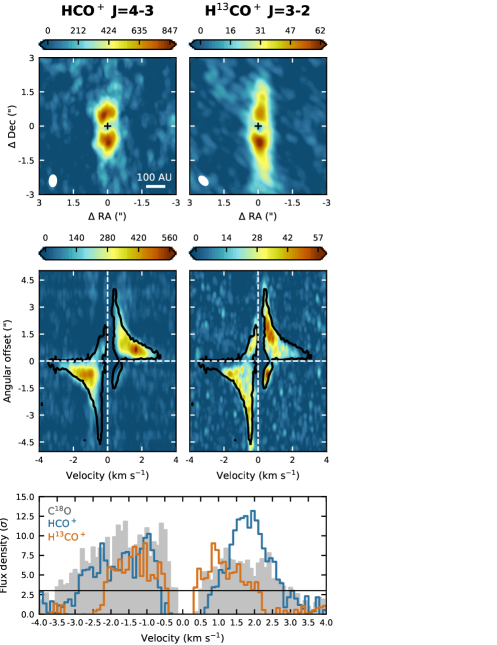
Figure 1: Integrated intensity maps (top) and position-velocity (pv) diagrams (middle) for the HCO⁺ $J=4-3$ (left) and H¹³CO⁺ $J=3-2$ (right) transitions toward L1527. Central velocity channels ($\Delta v\leq|0.5|$ km s^-1) with resolved out emission are omitted from the integrated intensity maps. The velocity axis of the pv diagrams is centered on the systemic velocity of 5.9 km s^-1 and the C¹⁸O $J=2-1$ pv diagram is overlaid in black contours (3$\sigma$). The color scale is in mJy beam^-1 km s^-1 for the integrated intensity maps and in mJy beam^-1 for the pv diagrams. The beam is shown in the bottom left corner of the top panels and the velocity resolution is 0.1 km s^-1. The bottom panel shows cuts through the pv diagrams close to the midplane ($0\farcs 2$ and -$0\farcs 2$ for, respectively, redshifted and blueshifted C¹⁸O and HCO⁺ emission, and $\pm 0\farcs 5$ for H¹³CO⁺) to highlight the difference in velocity extent between C¹⁸O (solid grey), HCO⁺ (blue line) and H¹³CO⁺ (orange line). The flux is expressed in factors of $\sigma$ for each dataset, and the horizontal line marks the $3\sigma$ level.

3 Results

Figure 1 (top panels) presents the integrated intensity maps for HCO⁺ $J=4-3$ and H¹³CO⁺ $J=3-2$ toward L1527. Emission from channels near the systemic velocity ($\Delta v\leq|0.5|$ km s^-1) where most of the emission is resolved out are omitted. Both molecules display emission elongated along the north-south direction, that is, along the major axis of the edge-on disk, with the blueshifted emission south of the protostar. The HCO⁺ emission is radially more compact than the H¹³CO⁺ emission, likely because the $J=4-3$ transition traces warmer and denser material than the $J=3-2$ transition. The higher sensitivity of the H¹³CO⁺ observations and more resolved out emission for the optically thicker HCO⁺ emission possibly play a role as well. For both lines, a central depression is visible, which at first thought may be interpreted as a lack of HCO⁺ and H¹³CO⁺ in the inner region of the disk. However, modeling of HCO⁺ emission by Hsieh et al. (2019) showed that a ring-shaped distribution of HCO⁺ molecules in an embedded disk does not result in a central depression in emission for highly inclined sources. For the edge-on disk L1527 the central depressions are thus due to a combination of optically thick continuum emission in the central beam, resolved out line emission and the subtraction of continuum from optially thick line emission.

A better picture of the spatial origin of the emission can be obtained from position-velocity (pv) diagrams as shown in Fig. 1 (middle panels). In principle, in these diagrams, disk emission is located at small angular offsets and high velocities, while envelope emission extends to larger offsets but has lower velocities. The pv diagrams show that the HCO⁺ emission peaks at angular offsets of $\sim$1^′′ and velocities between $\sim$1–2 km s^-1, while the H¹³CO⁺ emission peaks at larger offsets ($\sim$1.5–3^′′) and lower velocities ($\lesssim$1 km s^-1). The presence of an infalling envelope is also evident from the presence of redshifted emission on the predominantly blueshifted south side of the source and blueshifted emission in the north. These components are strongest for H¹³CO⁺. Together, this suggests that the HCO⁺ emission is dominated by the disk and innermost envelope and that the H¹³CO⁺ emission originates mostly at larger radii ($\gtrsim$ 140 au). However, if the emission is optically thick, emission observed at small spatial offsets from source center may in fact originate at much larger radii (see e.g., van ’t Hoff et al. 2018b), so the difference between HCO⁺ and H¹³CO⁺ can be partially due to an optical depth effect.

An absence of HCO⁺ inside the water snowline in the inner disk would show up in the pv diagram as an absence of emission at the highest velocities. Because at these highest velocities only emission from the disk, and not from the envelope, is present (see e.g., Fig. 7) this effect can still be visible even if the emission becomes optically thick in the envelope. As a reference, the 3$\sigma$ contour of C¹⁸O $J=2-1$ emission at comparable resolution ($0\farcs 43\times 0\farcs 28$) is overlaid on the HCO⁺ and H¹³CO⁺ pv diagrams. These C¹⁸O observations were previously presented by van ’t Hoff et al. (2018b), but to maximize the signal-to-noise ratio, we show here the combined data from the long and short baseline tracks of the observing program, while van ’t Hoff et al. (2018b) only used the long baseline executions. C¹⁸O is present throughout the entire disk, so an absence of HCO⁺ and H¹³CO⁺ emission at the highest C¹⁸O velocities signals a depression or absence of these molecules in the inner region of the disk. The highest blue- and redshifted velocities observed for C¹⁸O are $-3.6$ km s^-1 and $+3.0$ km s^-1, respectively, with respect to the source velocity. HCO⁺ reaches velocities close to the highest redshifted C¹⁸O velocity, that is, $-2.8$ and $+2.9$ km s^-1, while H¹³CO⁺ is confined between $-2.1$ and $2.2$ km s^-1 at the 3$\sigma$ level of the observations (see Fig.1, bottom panel).

A more quantitative constraint on the spatial origin of the emission can be set by considering the velocity structure. To calculate the velocity field, we adopt a Keplerian rotating disk with an outer radius of 125 au (Tobin et al., 2013) embedded in a rotating infalling envelope following the prescription by Ulrich (1976) and Cassen & Moosman (1981). We use a stellar mass of 0.4 $M_{\odot}$ as this was found to best reproduce ALMA observations of ¹³CO and C¹⁸O (van ’t Hoff et al., 2018b). This is slightly lower than the $\sim$0.45 $M_{\odot}$ derived by Aso et al. (2017). The resulting midplane velocity field is displayed in Fig. 7. For this stellar mass and disk radius, emission at velocities $\gtrsim|2.6|$ km s^-1 offset from the source velocity originates solely in the disk. The highest velocity HCO⁺ emission observed at the current sensitivity is predominantly coming from the disk at radii $\gtrsim$ 42 au. All H¹³CO⁺ velocity channels contain emission from both disk and envelope. This means that either the observed H¹³CO⁺ emission originates solely in the envelope, or there is some emission coming from the outer disk (radii $\gtrsim$ 73 au) as well. As illustrated in Fig. 7, these cases are not trivial to distinguish as the envelope velocity profile results in envelope emission being present at small angular offsets from the protostellar position. However, taken together, these results thus suggest an absence of HCO⁺ emission in the inner $\sim$40 au at the sensitivity of our observations.

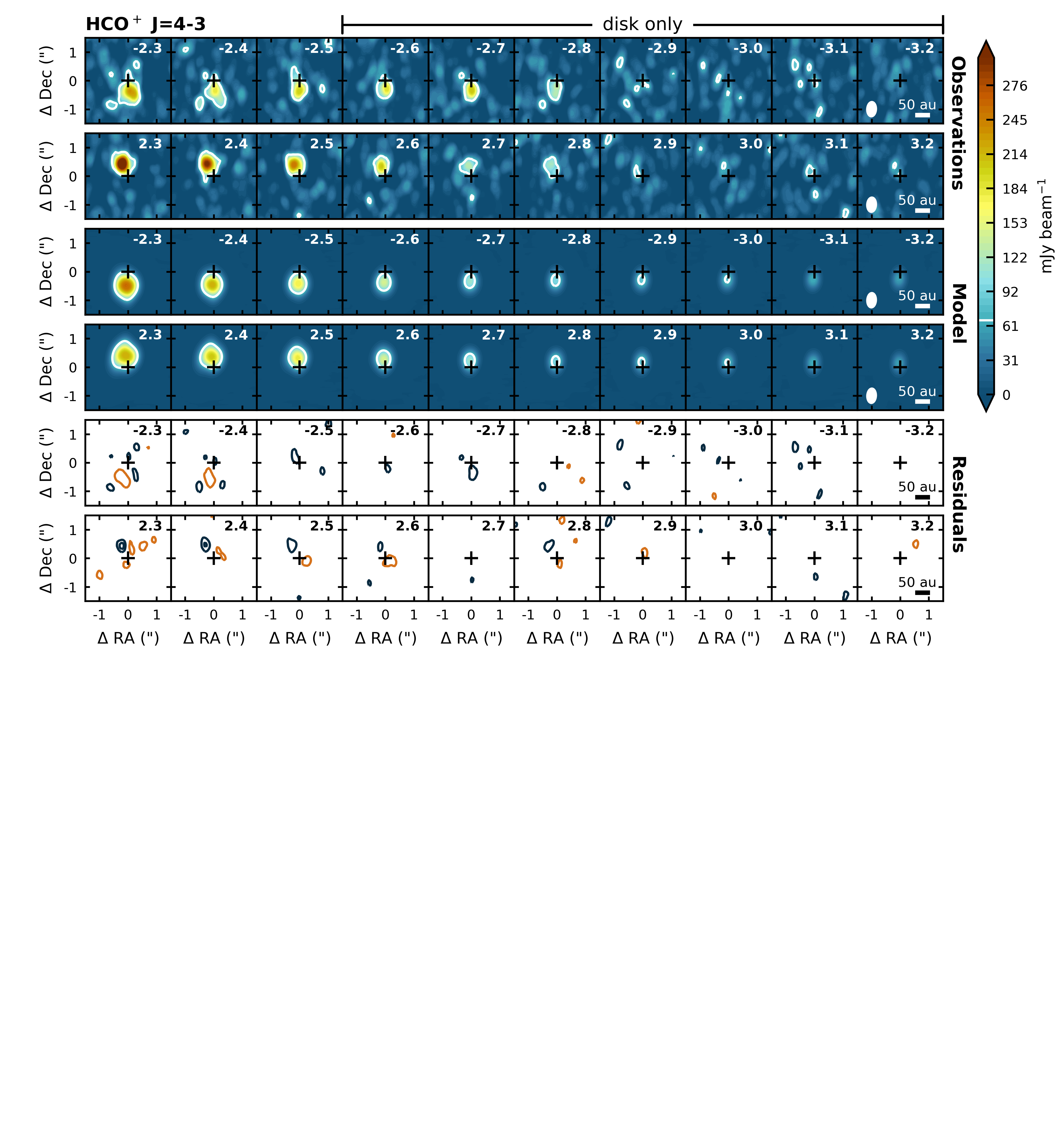
Figure 2: Selected channels of HCO⁺ $J=4-3$ emission from observations (top two rows) and from a L1527 specific model with an abundance of $2\times 10^{-11}$ at radii $\leq$60 au and an abundance of $2\times 10^{-10}$ at larger radii (middle two rows). The velocities offset from the source velocity (km s^-1) are listed in the top right corner of each panel, and channels at velocities $\gtrsim|2.6|$ km s^-1 contain only emission from the disk. A white contour denotes the 3$\sigma$ level. Residuals after subtracting the model from the observations are shown in the bottom two rows. Black contours are in steps of 3$\sigma$, starting at 3$\sigma$ and orange contours are in steps of -3$\sigma$ starting at -3$\sigma$. The black cross marks the continuum peak and the beam is shown in bottom left corner of the right most panels.

4 Modeling of the HCO⁺ emission

To further interpret these observations, we make synthetic HCO⁺ and H¹³CO⁺ images using the physical structure for L1527 derived by Tobin et al. (2013) and that was also used by van ’t Hoff et al. (2018b) and van ’t Hoff et al. (2020) to model the ¹³CO, C¹⁸O and C¹⁷O emission. In short, this model contains a 125 au Keplerian disk within a rotating infalling envelope (Ulrich, 1976; Cassen & Moosman, 1981) and is the result of fitting a large grid of 3D radiative transfer models to the thermal dust emission in the (sub-)millimeter, the scattered light $L^{\prime}$ image, and the multi-wavelength SED. In order to fit the multi-wavelength continuum emission, a parameterized sub/millimeter dust opacity was adopted with a value of 3.5 cm² g^-1 at 850 $\mu$m (Andrews & Williams, 2005) and the best fit model has a dust opacity spectral index $\beta$ of 0.25. This dust opacity suggests that some grain growth has occured (see Tobin et al. 2013 for more discussion). In our model, the dust then becomes optically thick at radii $\lesssim$4 au for different angular offsets along the disk major axis at the frequency of the HCO⁺ $J=4-3$ transition (356.734288 GHz) (see Fig. 7). The temperature and density structure of the model is shown in Fig. 9.

We employ two approaches to constrain the spatial origin of the HCO⁺ and H¹³CO⁺ emission and the water snowline location. First, we adopt a parametrized abundance structure where the HCO⁺ abundance is vertically constant but can change at different radii (Sect. 4.1). This simple type of model will allow us to address whether the non-detection of HCO⁺ and H¹³CO⁺ emission at velocities as high as observed for C¹⁸O is due to a steep drop in abundance, as expected inside the water snowline. Second, we use a small chemical network for HCO⁺ as presented by Leemker et al. (2021) for a more detailed study of the snowline location (Sect 4.2). In both cases, image cubes are simulated with the 3D radiative transfer code LIME (Brinch & Hogerheijde, 2010), assuming LTE and using molecular data files from the LAMDA database (Schöier et al., 2005; van der Tak et al., 2020). The synthetic image cubes are continuum subtracted and convolved with the observed beam size.

4.1 Parametrized abundance structure

Our goal here is to determine whether the absence of HCO⁺ and H¹³CO⁺ emission in the inner disk is due to a sharp drop in abundance, as expected inside the water snowline. We therefore parametrize the HCO⁺ abundance as function of radius and focus on the intermediate and high velocity channels that contain emission from the disk and inner envelope.

Velocity-channel emission maps of a model that reproduces the HCO⁺ emission at velocities $\geq|2.3|$ km s^-1 reasonably well are presented in Fig. 2. This model has a HCO⁺ abundance of $2\times 10^{-11}$ at radii $\leq$ 60 au, and an abundance of $2\times 10^{-10}$ at larger radii. This latter abundance is not high enough to reproduce the observed envelope emission at lower velocities, and this is most likely the reason that the redshifted emission at intermediate velocities (2.3–2.5 km s^-1) is slightly underestimated. However, the important result here is that the HCO⁺ abundance inside 60 au is low, and therefore, the non-detection of emission at velocities $\geq|2.9|$ km s^-1 (tracing the inner $\sim$40 au) could be due to the sensitivity of the observations. Abundances higher than $2\times 10^{-11}$ produce emission above the observed 3$\sigma$ level at velocities $\geq|2.9|$ km s^-1, but a further drop in abundance at radii $\lesssim$40 au cannot be assessed.

The abundance in the outer disk ($>$ 60 au) is hard to constrain as well, because the abundance in the outer disk and inner envelope are degenerate. A model with an abundance of $2\times 10^{-11}$ throughout the entire disk and an envelope abundance of $1\times 10^{-9}$ reproduces the observations equally well as the model displayed in Fig. 2. We can break this degeneracy using the H¹³CO⁺ observations. As shown in Fig. 10, the H¹³CO⁺ emission at velocities $\geq|1.9|$ km s^-1 can be reproduced by a model with a constant H¹³CO⁺ abundance of $3\times 10^{-12}$ in both disk and envelope. For an elemental ¹²C/¹³C ratio of 68 (Milam et al., 2005), an H¹³CO⁺ abundance of $3\times 10^{-12}$ suggests an HCO⁺ abundance of $2\times 10^{-10}$. Together these modeling results thus suggest that the HCO⁺ abundance is lower in the disk than in the envelope, with abundances of $2\times 10^{-10}$ in the outer disk ($>$ 60 au), $2\times 10^{-11}$ at 40–60 au, and $\leq 2\times 10^{-11}$ at radii $<$ 40 au.

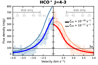
(a)

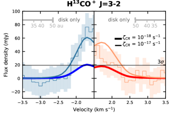
(b)

Figure 3: Spectra of the HCO⁺ (left panel) and H¹³CO⁺ (right panel) emission extracted in a 0$\farcs$75 aperture centered on the blueshifted emission peak (left sides of each panel) and on the redshifted emission peak (right sides of each panel). The observations are displayed in discrete velocity bins of 0.1 km s^-1 with the shaded area depicting the 3$\sigma$ uncertainty and a 10% flux calibration uncertainty. The smooth lines are for models with a CO abundance of 10^-4 and a H₂O abundance of 10^-6, but with varying cosmic ray ionization rates of 10^-18 s^-1 (thick line; referred to as the fidicial model) and 10^-17 s^-1 (thin line; canonical cosmic ray ionization rate). The horizontal black line marks the 3$\sigma$ level. The velocity range containing only emission from the disk is marked by grey bars in the top of the panels, and the maximum radius probed at certain velocities is indicated. The displayed velocity range is different for both molecules.

Jørgensen et al. (2004) derived an H¹³CO⁺ abundance of $8.5\times 10^{-12}$ for the envelope around L1527 from multiple single-dish observations. This is within a factor of three of our derived abundance of $3\times 10^{-12}$, and consistent with our result that the abundance increases at larger radii. Our derived HCO⁺ abundances on disk scales are consistent with the modeling results from Leemker et al. (2021) for protoplanetary disks around Herbig stars, which show a similar HCO⁺ abundance gradient in the outer disk (20–100 au) and a stronger decrease across the snowline (4.5 au) with the abundance dropping below $10^{-12}$. The current observations are not sensitive enough to constrain such low abundances. However, since the HCO⁺ abundance also depends on density and ionization, chemical modeling using a physical model specific for L1527 is required to link the abundance structure to the snowline.

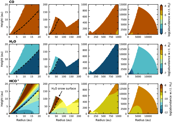
Figure 4: Abundance structure for CO (top panels), H₂O (middle panels) and HCO⁺ (bottom panels) predicted by the fiducial chemical model with initial CO and H₂O abundances of 10^-4 and 10^-6, respectively, and a cosmic ray ionization rate of $10^{-18}$ s^-1 for the physical structure of L1527. From left to right, panels display larger spatial scales. The disk outer radius is 125 au. The dashed line in the two left most columns marks the H₂O snow surface and the midplane snowline at 3.4 au.

4.2 Chemical modeling

The chemical network presented by Leemker et al. (2021) was developed to study the relationship between the water snowline and HCO⁺ (and H¹³CO⁺) emission in Herbig disks. It contains the main formation and destruction reactions for HCO⁺ as well as the freeze out and thermal desorption of water, as illustrated in Fig. 11. Reaction rate constants are taken from the UMIST database (McElroy et al., 2013), and are listed in Table 2 of Leemker et al. (2021). For water, a binding energy of 5775 K is used, which corresponds to an amorphous water ice (Fraser et al., 2001).

Freeze out of CO, the parent gas-phase molecule of HCO⁺, was not included in the study by Leemker et al. (2021) as this only occurred in the low-density outer region of the Herbig disks. Although there is no sign of CO freeze out in the disk around L1527 (van ’t Hoff et al., 2018b, 2020), we have added the freeze out and thermal desorption of CO to the chemical network for completeness and to display the HCO⁺ abundance structure in the envelope. The extact temperature at which CO desorbs depends on the composition of the ice (e.g., Collings et al., 2003), with pure CO ice desorbing at lower temperatures (855 K; Bisschop et al. 2006) than CO ice on top of water ice (1150 K; Garrod & Herbst 2006). The resulting desorption temperatures differ by $\sim$6 K; for example, 18 K versus 24 K for a density of $10^{7}$ cm^-3. In either case the CO snowline is located outside the L1527 disk, at $\sim$500 au or $\sim$200 au, respectively, and we adopt the binding energy of 855 K for a pure CO ice (Bisschop et al., 2006). Including or excluding freeze out of CO does not influence the HCO⁺ emission in the disk and inner envelope velocity channels that we are interested in here.

The freeze out rates depend on the available surface area of the dust grains. Following Leemker et al. (2021), we assume a typical grain number density of $10^{12}\times n$(H₂) and a grain size of 0.1 $\mu$m. Even if a fraction of the grains have grown to larger sizes, the smallest grains will dominate the surface area and van ’t Hoff et al. (2017) showed that adopting a more detailed description for the available surface area did not significantly affect the predicted N₂H⁺ abundance for the protoplanetary disk around TW Hya. For the radiative transfer, we use the dust opacities from Tobin et al. (2013) as described at the beginning of Sect. 4.

Initially, all abundances are set to zero, except for H₂, gas-phase CO and gas-phase H₂O, and we run the chemistry for $10^{5}$ year. Running the chemistry for $10^{6}$ year, as typically done for protoplanetary disk studies, does not affect the HCO⁺ abundance structure in the disk and inner envelope (radii $\lesssim$ 1000 au; see Appendix C). The main free parameters in the model are the initial CO and H₂O abundance and the cosmic ray ionization rate, which initiates the ion-neutral chemistry by ionizing H₂. The model does not include isotope-specific reactions and we adopt a ¹²C/¹³C ratio of 68 (Milam et al., 2005) to generate H¹³CO⁺ image cubes.

van ’t Hoff et al. (2018b) did not find evidence for a CO abundance much lower than the canonical value of $10^{-4}$ in the L1527 disk and Harsono et al. (2020) derived an upper limit for the H₂O abundance of $10^{-6}$. A model with these initial abudances reproduces the HCO⁺ and H¹³CO⁺ observations equally well as the parametrized model described in Sect. 4.1. For HCO⁺ a cosmic ray ionization rate of $10^{-18}$ s^-1 (about one order of magnitude below the canonical value) needs to be adopted (see Fig. 3). The asymmetry between blueshifted and redshifted emission is due to the kinematics of the disk and envelope, with the envelope in front of the disk for redshifted emission and the envelope behind the disk for blueshifted emission (see Appendix C). Since the HCO⁺ observations are more sensitive to the disk than the H¹³CO⁺ observations, as discussed in Sections 2 and 4.1, we will focus first on the model that reproduces the HCO⁺ emission and we will discuss the ionization rate in more detail in Sect. 5.2.

The abundance structure reproducing the HCO⁺ observations (our fiducial model with X(CO) = 10^-4, X(H₂O) = 10^-6 and $\zeta_{\rm{CR}}=10^{-18}$ s^-1) is presented in Fig. 4. For the adopted temperature and density structure, the water snowline is located at 3.4 au, which corresponds to a temperature of 140 K. The snow surface is located high up in the disk surface layers, making most of the disk and the inner envelope devoid of gas-phase water. Water is present in the gas phase at radii $\gtrsim$ 3000 au because the density in the outer envelope becomes too low for water to freeze out in the timescale of the model. A similar water abundance profile was found by Schmalzl et al. (2014), who used a simplified chemical network that was benchmarked against three full chemical networks to model Herschel observations of water in protostellar envelopes.

Overall, the HCO⁺ abundance gradually decreases with increasing density and steeply decreases across the water snow surface. At the high midplane densities, the HCO⁺ abundance remains low directly outside the water snowline as shown in earlier work (van ’t Hoff et al., 2018a; Hsieh et al., 2019). In the midplane, the HCO⁺ abundance drops from $10^{-11}$ at 16 au to $3\times 10^{-12}$ at 5 au and then steeply drops to abundances $<10^{-12}$ inside the snowline. These abundances are all at least an order of magnitude lower than the upper limit derived for the high velocity channels probing radii $\leq 40$ au using the parametrized model in Sect. 4.1. The sensitivity of the observations is thus not high enough to probe the HCO⁺ abundance drop across the snowline and the absence of emission in the highest velocity channels cannot be linked to the snowline. The high HCO⁺ abundance in the uppermost surface layers of the disk is likely because CO photodissociation is not included in the model. In this region, the rate for the reaction between HCO⁺ and H₂O, $R_{\mathrm{destruction}}$,

$$R_{\mathrm{destruction}}\propto n(\mathrm{HCO}^{+})n(\mathrm{H}_{2}\mathrm{O}),$$ (1)

is low, because the low density results in a low H₂O number density, $n$(H₂O). As discussed by Leemker et al. (2021), electron recombination becomes the dominant destruction mechanism of HCO⁺ in this region. At the same time, the HCO⁺ formation rate, $R_{\mathrm{formation}}$,

$$R_{\mathrm{formation}}\propto n(\mathrm{CO})n(\mathrm{H}_{3}^{+}),$$ (2)

remains high as the H${}_{3}^{+}$ number density is set by the cosmic ray ionization rate and is therefore independent of density. Including CO photodissociation would remove the parent molecule CO and hence prevent HCO⁺ formation, but knowledge of the UV field is required for a proper implementation. However, this low-density layer does not significantly contribute to the total HCO⁺ emission. Manually removing this layer before radiative transfer results in flux differences less than 0.2% and identical spectra as to those displayed in Fig. 3.

The HCO⁺ abundance is barely influenced by CO freeze out, because this occurs only in a small region of the envelope. In the disk and inner envelope ($\lesssim$900 au), the temperature is too high for CO to freeze out, while at radii $\gtrsim$2500 au the density becomes too low for CO to freeze out within $10^{5}$ yr, resulting in CO being present in the gas phase at the initial abundance throughout the majority of the system. A similar abundance profile was derived by Jørgensen et al. (2005) for a sample of 16 sources, and ¹³CO has been observed out to radii of $\sim$10,000 au toward L1527 (Zhou et al., 1996). Running the chemistry for $10^{6}$ yr results in a midplane region with a decreased HCO⁺ abundance centered around 2500 au due to higher levels of CO freeze out. Simultaneously, the higher levels of H₂O freeze out increase the HCO⁺ abundance, resulting overall in only a small region with a lower HCO⁺ abundance at radii $\gtrsim$1000 au after $10^{6}$ year. The HCO⁺ abundance at smaller radii is unaffected (see Fig. 12).

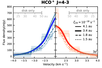
(a)

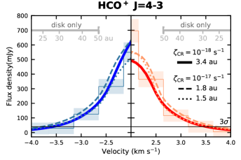
(b)

Figure 5: Spectra of the HCO⁺ emission extracted in a 0$\farcs$75 aperture centered on the blueshifted emission peak (left side of each panel) and on the redshifted emission peak (right side of each panel). The observations are binned to 0.5 km s^-1 and the shaded area depicts the 3$\sigma$ uncertainty and a 10% flux calibration uncertainty. The thick dark colored lines are for the fiducial model with a snowline at 3.4 au. The other lines represent models where the disk temperature has been multiplied by a constant factor to obtain snowline locations of 1.5 au (dotted line), 1.8 au (dashed line) and 4.1 au (thin solid line). The cosmic ray ionization rate is $10^{-18}$ s^-1 for the models in the left panel and $10^{-17}$ s^-1 in for the models in the right panel, except for the fiducial model (thick line) which is the same as in the left panel. The horizontal black line marks the 3$\sigma$ level. The velocity range containing only emission from the disk is marked by grey bars in the top of the panels, and the maximum radius probed at certain velocities is indicated.

The HCO⁺ abundance structure in the disk as presented in Fig. 4 is very robust with respect to changes in the initial CO and H₂O abundance. Aso et al. (2017) suggested a CO abundance of $2\times 10^{-5}$ based on ALMA observations of C¹⁸O, but lowering the CO abundance two orders of magnitude does not affect the HCO⁺ abundance in the disk significantly (see Fig. 13). The only changes are a lower HCO⁺ abundance in the upper most surface layers of the disk (above the snow surface) and a lower abundance at radii $\gtrsim$900 au. A canonical H₂O abundance of $10^{-4}$ increases the vertical height of the HCO⁺ depleted layer above the snow surface and strongly decreases the HCO⁺ abundance at radii $\gtrsim$1500 au (see Fig. 14). Lowering the H₂O abundance further to $10^{-7}$ slightly increases the HCO⁺ abundance above the snow surface. The HCO⁺ abundance thus remains unaltered throughout the majority of the disk for CO abundances between $10^{-4}$ and $10^{-6}$ and H₂O abundances between $10^{-4}$ and $10^{-7}$.

The only parameter that has a strong impact on the HCO⁺ abundance in the disk is the cosmic ray ionization rate. As described in van ’t Hoff et al. (2018a), the HCO⁺ abundance is proportional to the square root of the cosmic ray ionization rate. Hence, a canonical value of $10^{-17}$ s^-1 results in a HCO⁺ abundance higher by a factor $\sim$3 compared to a rate of $10^{-18}$ s^-1 (Fig. 15 versus Fig. 4), and a too high HCO⁺ flux compared to what is observed (see Fig. 3). The predicted HCO⁺ flux for a CR ionization rate of $10^{-17}$ s^-1 is less than a factor 3 higher than the flux predicted for a rate of $10^{-18}$ s^-1, signaling that the emission becomes optically thick.

5 Discussion

5.1 The water snowline location in L1527

For the temperature and density structure derived by Tobin et al. (2013), the water snowline is predicted to be at 3.4 au in the disk around L1527 and the corresponding HCO⁺ abundance structure from a small chemical network calculation can reproduce the observed HCO⁺ emission. Although the current observations are not sensitive to the expected HCO⁺ abundance changes across the snowline, the chemical model shows a decrease in the HCO⁺ abundance over a much larger radial range above the snow surface. This suggests that the snowline location may be constrained indirectly from HCO⁺ emission based on the global temperature structure. To investigate the stringency of the current observations, we run a set of models with different snowline locations separated by $\sim$0.2–0.5 au generated by multiplying the fiducial temperature structure in the disk by a constant factor. To obtain the maximum sensitivity, we bin the observations to 0.5 km s^-1.

Figure 5 displays the HCO⁺ spectra for models with a snowline at 1.5, 1.8, 3.4 (fiducial) and 4.1 au. The differences between these models are too small to be distinguished at disk-only velocities, but the current sensitivity is high enough to see a significant difference at a $\pm$2.4 km s^-1 velocity offset. While a snowline at 1.8 au produces HCO⁺ emission at about the 3$\sigma$ uncertainty level (including a 10% flux calibration uncertainty), a snowline at 1.5 au clearly underproduces the emission. The effect of a warmer disk is not very pronounced at redshifted velocities, but a snowline at 4.1 au slightly overproduces the blueshifted emission. Lower HCO⁺ emission as a result of a colder disk can partially be compensated by a higher cosmic ray ionization rate. For $\zeta_{\rm{CR}}=10^{-17}$ s^-1, a snowline at 1.5 au can reproduce the observed HCO⁺ emission, while a snowline at 1.8 au results in a too high flux. However, van ’t Hoff et al. (2018b) was not able to reproduce the ¹³CO and C¹⁸O $J=2-1$ emission with the temperature structure corresponding to a 1.5 au snowline (their Intermediate Model), instead requiring a warmer disk. Changing the temperature also in the envelope has only a small effect on the emission at $\pm$2.4 km s^-1 (Fig. 8). Taken together, for the here adopted physical structure, these results thus suggest a snowline radius of 1.8-4.1 au if $\zeta_{\rm{CR}}=10^{-18}$ s^-1 and between 1.5 and 1.8 au for $\zeta_{\rm{CR}}=10^{-17}$ s^-1.

No other molecular line observations are currently available to locate the water snowline in L1527: H${}_{2}^{18}$O emission has not been detected (Harsono et al., 2020), and while weak methanol emission has been observed, the sensitivity and resolution of that data were insufficient to determine its spatial origin (Sakai et al., 2014). Aso et al. (2017) presented a warmer model based on fitting of sub-millimeter continuum visibilities than the model derived by Tobin et al. (2013) and used in this work, with the snowline at $\sim$8 au. This is at least twice as far out as predicted here based on the HCO⁺ models, but the temperature profile is kept fixed in the fitting procedure of Aso et al. (2017). van ’t Hoff et al. (2018b) inferred a temperature profile based on optically thick ¹³CO and C¹⁸O emission, which has a temperature of $\sim$35 K at 40 au. The temperature in the inner $\sim$20 au depends strongly on the chosen power-law coefficient and does not provide a strong constraint on the snowline location.

Providing stronger constraints on the snowline location using HCO⁺ emission will require significantly deeper observations as illustrated in Fig. 6. As higher velocities trace emission originating out to smaller radii, the total flux decreases at higher velocities, and hence higher sensitivity is required to distinguish two models. Ideally, one would want to compare the flux in a certain velocity channel with the flux of models with the snowline inside and outside the maximum radius probed by that velocity. However, it is immediately clear from Fig. 6 that this is not possible for L1527 with current facilities as flux differences at $\gtrsim|4.0|$ km s^-1 (corresponding to a $\sim$20 au radius) become too small to be observed in 20 hours on source with ALMA.

Nonetheless, deeper integrations will allow for better constraints in two ways. First, a higher sensitivity will allow different models to be compared over more velocity channels, and in particular, in channels that only trace disk emission. This will remove any influence from the envelope. For example, 10 hours on source with ALMA will result in 5–10 0.1 km s^-1 disk-only channels (or 2–3 channels at 0.5 km s^-1) where models with snowlines at 1.8, 3.4 and 4.1 au can be distinguished, as compared to currently one 0.5 km s^-1 channel containing emission from both disk and envelope. Second, a higher sensitivity will allow to distinguish between models with smaller differences in snowline radius. With 10 hours on source, the snowline can be constrained within a few tenths of an au, although there will be a degeneracy with the cosmic ray ionization rate.

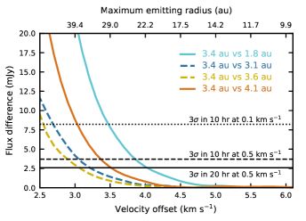
Figure 6: Difference in HCO⁺ $J=4-3$ flux between models with different snowline locations compared to the fiducial model with the snowline at 3.4 au at velocity offsets that trace only the disk. The top horizontal axis shows the maximum radius probed at a certain velocity for an edge-on Keplerian disk around a 0.4 $M_{\odot}$ star as used for L1527. The dotted and dashed lines mark the 3$\sigma$ limit that can be reached with ALMA in 10 hours on source at a spectral resolution of 0.1 and 0.5 km s^-1, respectively. The solid line is the 3$\sigma$ limit at 0.5 km s^-1 for 20 hours on source. The 3$\sigma$ sensitivity of the current HCO⁺ observations is 40 mJy at 0.5 km s^-1.

Higher J transitions will generally trace warmer and denser material, but in turn, higher dust opacity at higher frequencies may prevent to observe these transitions from the inner disk. For the here adopted dust opacities, the continuum $\tau=1$ surface shift outward by only $\sim$1 au for the $J=8-7$ transition (713.342090 GHz) compared to the $J=4-3$ transition (356.734288 GHz) (Fig. 7), suggesting that the dust opacity is not a strong limiting factor in choosing an HCO⁺ transition. For proper treatment of higher $J$ transitions, UV heating of the gas has to be taken into account and this emission may arise from a thin layer in which the gas and dust temperatures are decoupled (e.g., Visser et al., 2012). Such a modeling approach was adopted by Leemker et al. (2021), while we here adapt the dust temperature structure for L1527 and assume the gas and dust temperature are equal, which is appropriate for the $J=4-3$ transition which emits from regions where the temperatures are coupled (e.g., Mathews et al., 2013).

That being said, in our model the integrated flux at high velocities ($\gtrsim|3|$ km s^-1) increases up to a factor $\sim$2 or $\sim$3 for the $J=5-4$ (445.902996 GHz) and $J=7-6$ (624.208673 GHz) transitions, respectively, compared to the $J=4-3$ flux in the fiducial model (not shown). The flux of the $J=8-7$ transition is similar to the $J=7-6$ flux at velocities originating solely in the disk. For the $J=7-6$ transition, the curves in Fig. 6 shift to the right by $\sim$1 km s^-1, suggesting that it is easier to distinguish between different snowline locations. However, the decrease in atmospheric transmission results in significantly lower sensitivities that make high sensitivity observations very expensive: in 20 hours on source at 0.5 km s^-1 resolution, an rms of 224 mJy, 25 mJy and 20 mJy is reached for $J=5-4$, $J=7-6$, and $J=8-7$, respectively. These sensitivities would just be enough to distinguish between a snowline at 1.8, 3.4 or 4.1 au at velocity offsets $<$ 3 km s^-1 with the $J=7-6$ and $J=8-7$ transitions. As even for the $J=1-0$ (89.188523 GHz) transition the snowline coincides with the dust $\tau=1$ surface, the HCO⁺ $J=4-3$ transition is the best suited to constrain the snowline location.

With such long integration times required to derive stronger constraints on the snowline location from HCO⁺ emission, it is worth investigating whether the snowline can be located directly with water observations. As shown in Fig. 7, the snowline is expected to be hidden behind optically thick dust for frequencies above $\sim$90 GHz, so a direct detection of the snowline would not be possible for L1527. However, locating the snowline directly with water observations may still turn out to be a viable route for sources that have the water snowline extend beyond the radius where the dust becomes optically thick.

5.2 Cosmic ray ionization rate

Another important result concerns the cosmic ray ionization rate in the disk of L1527. The cosmic ray ionization rate is crucial for both the physical and chemical evolution of the disk. From a physical perspective, ionization plays an important role in angular momentum transport through the magneto-rotational instability (MRI; e.g., Balbus & Hawley 1991). From a chemical point of view are cosmic rays the driver of chemistry in the disk midplane, where other ionizing agents cannot penetrate (e.g., Eistrup et al., 2016, 2018). For the here adopted physical structure of L1527 that is able to reproduce multi-wavelength continuum emission (Tobin et al., 2013) as well as CO isotopologue emission (van ’t Hoff et al., 2018b), a canonical CR ionization rate of $10^{-17}$ s^-1 overproduces the HCO⁺ emission which originates predominantly from radii $\gtrsim$40 au (Fig. 3). The H¹³CO⁺ emission, which is originating predominantly from the inner envelope, does require a CR ionization rate of $10^{-17}$ s^-1 (Fig. 3).

In order to reproduce the HCO⁺ observations with a CR ionization rate of $10^{-17}$ s^-1 the disk temperature needs to be lowered such that the snowline is located inside of 1.8 au (instead of 3.4 au; Fig. 5). A temperature structure obtained by multiplying our fiducial temperature with a constant factor of 0.6, resulting in a snowline at 1.5 au, is too cold to explain the ¹³CO and C¹⁸O $J=2-1$ emission (van ’t Hoff et al., 2018b), but the CO isotopologue observations are not sensitive enough to confidently say whether the temperature structure associated with a 1.8 au snowline is too cold as well. We have assumed that the temperature changes globally by a constant factor, and this analysis cannot rule out that a model with a slightly flatter temperature profile (i.e., colder in the inner few au) would be able to explain the molecular line observations with a canonical CR ionization rate. Higher sensitivity observations of CO isotopologues or other temperature tracers are required to better constrain the detailed temperature structure.

A snowline location different from 3.4 au could be obtained by, for example, a different luminosity or different disk mass. Measurements of the bolometric luminosity based on the spectral energy distribution (SED) range between 1.6 and 2.0 $L_{\odot}$ (Tobin et al., 2008; Green et al., 2013; Karska et al., 2018). This is likely an underestimation of the true luminosity as edge-on sources embedded in an envelope can have internal luminosities up to $\sim$2 times higher than the bolometric luminosity (Whitney et al., 2003). For a 1 $L_{\odot}$ protostar, Tobin et al. (2008) require an accretion luminosity of 1.6 $L_{\odot}$ to fit the SED, resulting in a true bolometric luminosity of $\sim$2.6 $L_{\odot}$. The model used here has a total luminosity of 2.75 $L_{\odot}$ (Tobin et al., 2013), and assuming that the snowline radius scales as the square root of the luminosity, a luminosity of 0.8 $L_{\odot}$ would be required for a snowline radius of 1.8 au. This is a factor two smaller than derived from the SED. A lower disk mass could also shift the snowline inward, but for an accretion rate of $3\times 10^{-7}M_{\odot}$ yr^-1 (corresponding to an accretion luminosity of 1.6 $L_{\odot}$), models by Harsono et al. (2015) show less than 1 au difference between disk masses of 0.05 and 0.1 $M_{\odot}$. The disk mass of the model used here is 0.0075 $M_{\odot}$. Modeling of high resolution ALMA data, for example, from the FAUST or eDisk large programs may provide additional constraints on the disk structure.

Chemically, a canonical CR ionization rate may be reconciled with the observations if there is a higher destruction rate of HCO⁺. In our model, HCO⁺ can be destroyed by H₂O and electrons, where the electrons are provided by ionization of H₂ by cosmic rays. Since grains are likely negatively charged (Umebayashi & Nakano, 1980), ions may also recombine on dust grains. The recombination rate for this process, $R_{\mathrm{grain}}$, is given by

$$R_{\mathrm{grain}}=a_{g}n_{\mathrm{H}}n(\mathrm{HCO}^{+}),$$ (3)

where $a_{g}$ is the recombination rate coefficient ($a_{g}\approx 10^{-17}$ cm³ s^-1; Umebayashi & Nakano 1980), and $n_{\mathrm{H}}$ and $n(\mathrm{HCO}^{+})$ are the hydrogen and HCO⁺ number density. The recombination rate in the gas phase, $R_{\mathrm{gas}}$, is given by

$$R_{\mathrm{gas}}=kn_{\mathrm{e}}n(\mathrm{HCO}^{+}),$$ (4)

where $n_{\mathrm{e}}$ is the eletron density. The reaction rate coefficient, $k$, has a temperature dependence, and is $4-8\times 10^{-7}$ cm³ s^-1 for temperatures between 150 and 50 K (UMIST database; McElroy et al. 2013). This means that the grain recombination rate becomes larger than the gas-phase recombination rate for electron abundances, $n_{\mathrm{e}}/n_{\mathrm{H}}$, $\gtrsim$10^-11. Since the electron abundance is approximately equal to the HCO⁺ abundance, this condition is only met in the disk midplane inside $\sim$16 au for the fiducial model (Fig. 4) and only inside $\sim$5 au for the model with a CR ionization rate of $10^{-17}$ s^-1 (Fig. 15). Destruction of HCO⁺ via electron recombination on grains is thus unlikely to effect the predicted HCO⁺ abundance.

While we cannot fully rule out a canonical CR ionization rate, the different ionization rates derived from HCO⁺ and H¹³CO⁺ are not necessarily in conflict with each other. The lower $J$ transition and lower velocities probed with H¹³CO⁺ make the H¹³CO⁺ observations more sensitive to the inner envelope than the HCO⁺ observations. This would then suggest that the CR ionization rate is lower in the disk compared to the envelope, which could simply be the result of stronger attenuation of external cosmic rays due to the higher density of the disk. The cosmic ray ionization rate is expected to decrease exponentially with an attenuation column of 96 g cm^-2 (Umebayashi & Nakano, 1981, 2009) or even higher (Padovani et al., 2018). However, a column larger than 96 g cm^-2 is only reached in the inner 0.5 au in our L1527 model. Another explanation for a low cosmic ray ionization rate in the disk may be the exclusion of cosmic rays by stellar winds and/or magnetic fields as proposed by Cleeves et al. (2015) for the protoplanetary disk around TW Hya. The same mechanism could explain the gradient in cosmic ray ionization rate derived for the IM Lup disk, where the steep increase in CR ionization rate in the outer disk may indicate the boundary of the “T Tauriosphere”, that is, a stellar-wind-induced boundary analogous to the Sun’s heliosphere (Seifert et al., 2021).

While models show that cosmic rays can be produced by jet shocks and by accretion shocks at protostellar surfaces (Padovani et al., 2015, 2016), the transport of cosmic rays in protostellar disks is very complicated (as shown for external CRs by Padovani et al. 2018). Models by Gaches & Offner (2018) for the simpler case of protostellar cores show five orders of magnitude difference in CR ionization rate between the two limiting cases of transport of internally created CRs through the core.

In our chemical network, all ionization is provided by cosmic rays, but UV and X-ray ionization can play a role as well, in particular in higher layers in the disk with X-rays penetrating deeper than UV radiation (see e.g., Cleeves et al. 2014; Notsu et al. 2021; Seifert et al. 2021). However, it is not clear at what point during stellar evolution the dynamo turns on and X-rays are emitted, and no X-ray emission has been detected toward L1527 with Chandra (Güdel et al., 2007). Since the observations constrain the HCO⁺ abundance, a significant contribution of UV and/or X-rays to the HCO⁺ chemistry would mean that the cosmic ray ionization rate is even lower than $10^{-18}$ s^-1.

Other observational constraints for the CR ionization rate in the L1527 disk do not currently exist. Favre et al. (2017) used Herschel observations of the ratio between HCO⁺ $J=6-5$ and N₂H⁺ $J=6-5$ to constrain the ionization rate in Class 0 protostars, but the upper limit resulting from the non-detection of N₂H⁺ toward L1527 only constrains the CR ionization rate to be smaller than $10^{-14}$ s^-1. The signal-to-noise ratio of the $J=6-5$ observations is too low to detect emission at velocity offsets $\gtrsim$2 km s^-1, so they do not help in constraining the HCO⁺ distribution or disk temperature structure.

If confirmed, a low CR ionization rate in a young disk may have profound consequences as high ionization levels are crucial for disk evolution. For example, for angular momentum transport through MRI, the gas needs to be coupled to the magnetic field (Gammie, 1996), and hence insufficient ionization may suppress MRI and create a low-turbulence “dead zone”, favorable for planetesimal formation (e.g., Gressel et al., 2012). From a chemical perspective, the up to two orders of magnitude CO depletion observed in protoplanetary disks can only be reproduced by models with CR ionization rates on the order of $10^{-17}$ s^-1 (Bosman et al., 2018; Schwarz et al., 2019). Currently the CO snowline is located outside the L1527 disk (van ’t Hoff et al., 2018b), but unless the CR ionization rate would increase at later stages, a CR ionization rate of $10^{-18}$ s^-1 would suggest that no chemical processing of CO will occur in the L1527 disk once the disk has cooled enough for the CO snowline to shift inward.

6 Conclusions

We have presented $\sim 0\farcs 5$ ($\sim$70 au) resolution ALMA observations of HCO⁺ $J=4-3$ and H¹³CO⁺ $J=3-2$ toward the embedded disk L1527. In order to constrain, for the first time, the water snowline location in a young disk, we modeled the HCO⁺ abundance and emission using a physical model specific for L1527 (Tobin et al., 2013) and a small chemical network (based on Leemker et al. 2021). Our main results are summarized below.

• The observed HCO⁺ emission traces the disk down to a radius of $\sim$40 au. The emission can be reproduced with the L1527-specific physical structure that has the water snowline at 3.4 au, given that the cosmic ray ionization rate is lowered to $10^{-18}$ s^-1.

• Even though the observations are not sensitive to the expected HCO⁺ abundance change across the midplane snowline, the change across the radial snow surface and the global temperature structure allow us to constrain the snowline location between 1.8 and 4.1 au by multiplying the fidicial temperature structure with a constant factor. The snowline can be inward of 1.8 au if the CR ionization rate is $10^{-17}$ s^-1, but a previous analysis showed that a temperature structure with the snowline at 1.5 au is too cold to reproduce the ¹³CO and C¹⁸O observations.

• The HCO⁺ abundance structure in the disk predicted by the small chemical network is very robust for the initial H₂O and CO abundance, and only significantly depends on the cosmic ray ionization rate.

• The observed H¹³CO⁺ emission extends out to lower velocity offsets than the HCO⁺ emission, indicating that the emission predominantly originates in the inner envelope. For the adopted physical structure, a canonical CR ionization rate of $10^{-17}$ s^-1 is required to reproduce the H¹³CO⁺ emission. Together, the HCO⁺ and H¹³CO⁺ results suggest that the CR ionization rate has a canonical value of $10^{-17}$ s^-1 in the inner envelope and may be attenuated to $\sim 10^{-18}$ s^-1 in the disk.

These results demonstrate the use of HCO⁺ as a snowline tracer in embedded disks. However, as long integration times with ALMA are required to detect emission at high velocities to eliminate envelope contribution and to constrain the snowline to within 0.5 au, the direct detection of the snowline through observations of water isotopologues may still prove to be a viable strategy. Deep water observations of a range of different sources are required to constrain when water observations are viable and when we have to retort to indirect tracing with HCO⁺. Observations of water ice with the James Webb Space Telescope may provide constraints on the (vertical) snowline as well. In sources with a direct measurement of the snowline location, HCO⁺ observations will allow to constrain the cosmic ray ionization rate.

Appendix A Physical and kinematical structure of L1527

Figure 7 presents the velocity along the line of sight for the material in the disk and inner envelope midplane. The highest velocities are only reached in the inner disk, presenting an opportunity to study disk emission unaffected by the envelope. At intermediate velocities ($\Delta|v|\sim 1.6-2.6$ km s^-1), redshifted emission from the envelope originates in front of the disk, while at blueshifted velocities we see the disk in front of the envelope. This can result in asymmetric line profiles, as for example in Fig. 3, especially when the emission becomes optically thick. For HCO⁺, we can illustrate this clearly by comparing models where the temperature modification as described in Sect. 5.1 is applied only to the disk or to both the disk and envelope. As can be seen in Fig. 8, the blueshifted emission at velocities $\leq-2.0$ km s^-1 is hardly affected by a change in envelope temperature, signaling that most of the emission is originating in the disk. The redshifted emission is stronger affected and the redshifted emission at velocities $\leq 2.5$ km s^-1 thus has a strong envelope component. Another effect that comes in to play at lower redshifted velocities is absorption due to the foreground infalling envelope. This effect together with larger scale emission being resolved out may explain why the model better reproduces the blueshifted H¹³CO⁺ emission as the convolution of the synthetic image cube does not capture the effects of the interferometer.

Figure 7 also shows the location where the dust emission becomes optically thick along the midplane (that is, along the north-south direction) in our model. We adopt a parametrized dust opacity with a value of 3.5 cm² g^-1 at 850 $\mu$m and a spectral index $\beta$ of 0.25 (Tobin et al., 2013). At the frequency of the HCO⁺ $J=4-3$ transition (356.734288 GHz; as observed), the dust becomes optically thick just outside the snowline. Even for the lowest HCO⁺ transition ($J=1-0$ at 89.188523 GHz) the snowline coincides or falls just inside of the $\tau=1$ surface and will be hidden by the dust.

The temperature and density structure in the adopted physical model for L1527 is shown in Fig. 9. This model was derived by Tobin et al. (2013) using a large grid of 3D radiative transfer models to model the thermal dust emission in the (sub-)millimeter, the scattered light $L^{\prime}$ image, and the multi-wavelength SED. The model includes a rotating infalling envelope (Ulrich, 1976; Cassen & Moosman, 1981) and a flared disk (e.g., Hartmann et al., 1998). In addition to a protostellar luminosity of 1.0 $L_{\odot}$, a luminosity of 1.75 $L_{\odot}$ is used to account for the accretion from the disk onto the protostar.

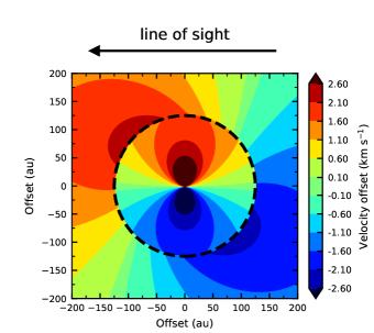
(a)

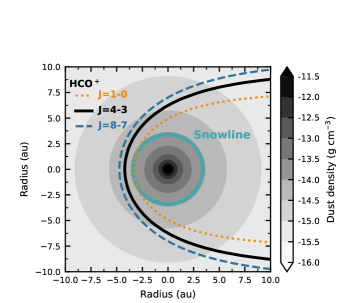
(b)

Figure 7: Left panel: Face-on view of the midplane in the disk and inner envelope of L1527, showing the velocity component along the line of sight (the observer is on the left as indicated by the black arrow above the panel). The material in the 125 au disk (marked by a dashed line) has a Keplerian velocity, while the envelope material has a rotating infalling velocity profile (Ulrich, 1976; Cassen & Moosman, 1981). The adopted stellar mass is 0.4 $M_{\odot}$. Right panel: Dust density in the inner 10 au and the $\tau$ = 1 surfaces for the dust emission in our model at the wavelengths of the HCO⁺ $J=1-0$ (89.188523 GHz; dotted orange line), $J=4-3$ (356.734288 GHz; solid black line) and $J=8-7$ (713.342090 GHz; dashed blue line) transitions. The snowline at 3.4 au is indicated by the blue circle.

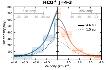
Figure 8: Spectra of the HCO⁺ emission extracted in a 0$\farcs$75 aperture centered on the blueshifted emission peak (left) and on the redshifted emission peak (right). The observations are binned to 0.5 km s^-1 and the shaded area depicts the 3$\sigma$ uncertainty and a 10% flux calibration uncertainty. The solid lines are for models with a snowline at 4.6 au and the dotted lines are for models with a snowline at 1.5 au. For the colored lines, the temperature factor required for that particular snowline location has only been applied to the disk, while for the gray lines, this temperature factor has been applied to both disk and envelope. The difference between colored and gray lines is thus only the temperature in the envelope. The horizontal black line marks the 3$\sigma$ level. The velocity range containing only emission from the disk is marked by grey bars in the top of the panels, and the maximum radius probed at certain velocities is indicated.

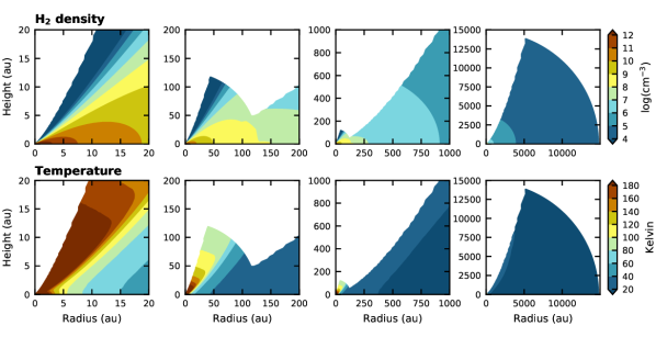
Figure 9: Density (top panels) and temperture (bottom panels) structure for the disk and envelope of L1527 from the best fit model by Tobin et al. (2013). From left to right, panels display larger spatial scales. The disk outer radius is 125 au.

Appendix B Parametrized modeling of H¹³CO⁺ emission

The H¹³CO⁺ observations can be reproduced by a constant abundance of $3\times 10^{-12}$, as presented in Fig. 10. This breaks the degeneracy between a HCO⁺ model with an abundance of $2\times 10^{-11}$ at radii $\leq$60 au and an abundance of $2\times 10^{-10}$ at larger radii (as shown in Fig. 2) and a model with an abundance of $2\times 10^{-11}$ in the entire 125 au disk and an abundance of $1\times 10^{-9}$ in the envelope, as the H¹³CO⁺ observations are in better agreement with the former HCO⁺ abundance structure.

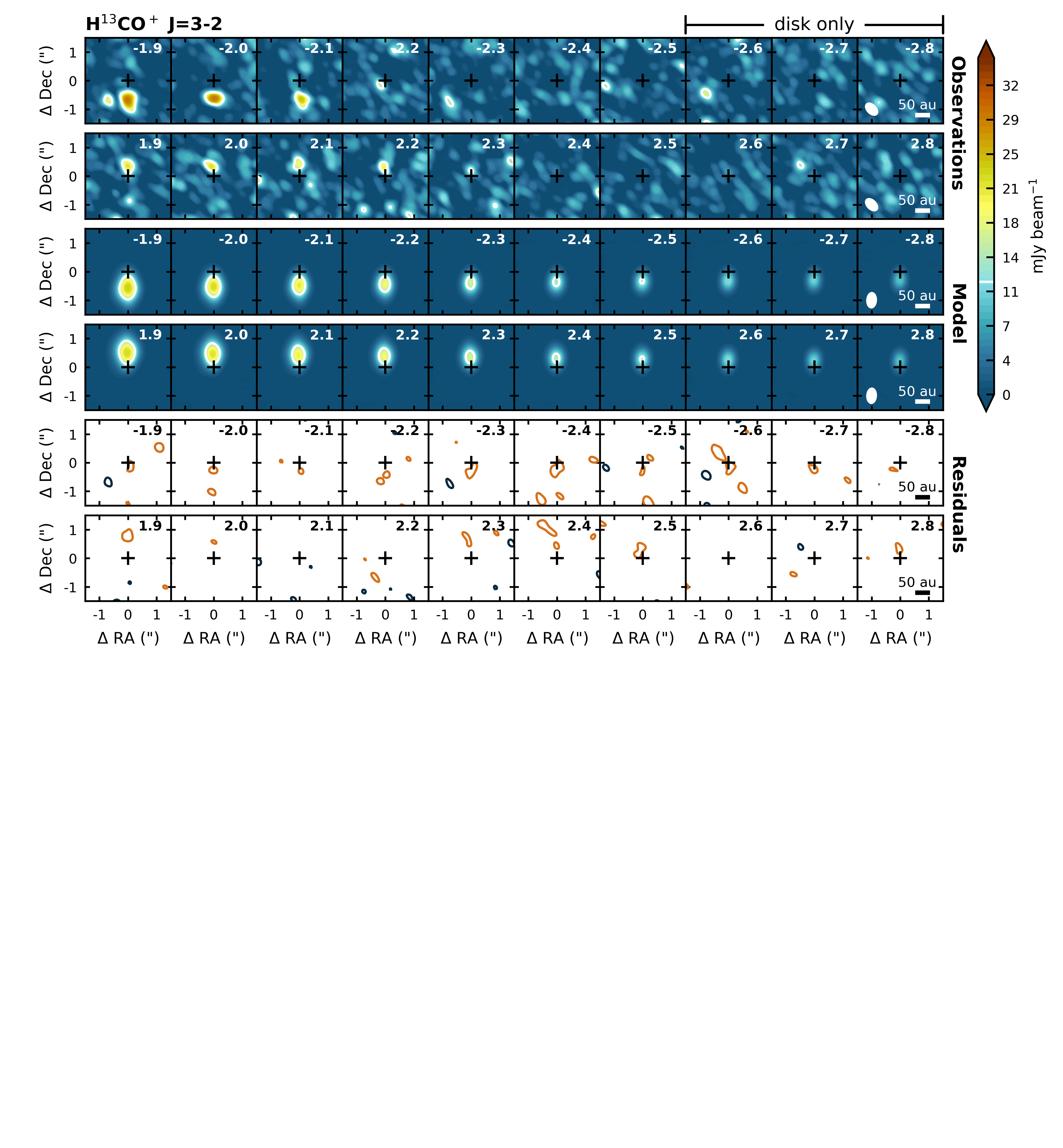
Figure 10: As Fig. 2, but for H¹³CO⁺ emission. The model has a constant abundance of $3\times 10^{-12}$. The depicted velocity range is slightly different from that shown for HCO⁺ in Fig. 2, because the H¹³CO⁺ emission is only detected at slightly lower velocities.

Appendix C Chemical modeling of HCO⁺ emission

Figure 11 shows a schematic of the chemical network used to model HCO⁺ and its relation with the water snowline using the physical structure of L1527, as shown in Fig. 9. The chemistry is evolved for a duration of $10^{5}$ yr, but for comparison, Fig. 12 shows the HCO⁺ abundance for the fiducial initial conditions of X(CO) = $10^{-4}$, X(H₂O = $10^{-6}$ and a CR rate of $10^{18}$ s^-1 after $10^{6}$ yr. The HCO⁺ abundance after $10^{5}$ yr but for different initial conditions are presented in Figs. 13-15: a low CO abundance of $10^{-6}$ (Fig. 13), a high H₂O abundance of $10^{-4}$ (Fig. 14) and a CR rate of $10^{17}$ s^-1 (Fig. 15).

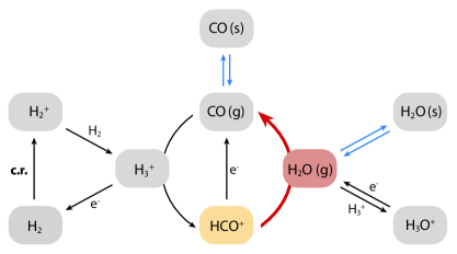
Figure 11: Schematic representation of the chemical network used to model HCO⁺ (orange). The reaction responsible for the anti-correlation between HCO⁺ and H₂O is highlighted with a red arrow. Freeze out and thermal desorption reactions are marked by blue arrows, where ‘g’ denotes gas-phase species and ‘s’ denotes ice species. Ionization of H₂ by cosmic rays (c.r.) initiates the ion-neutral chemistry. Leemker et al. (2021) did not include the freeze out of CO, because their disks were too warm for CO ice. Parameters that are adjusted in this work are the initial CO and H₂O abundances and the cosmic ray ionization rate.

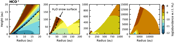
Figure 12: Abundance structure for HCO⁺ for the fiducial model (initial CO and H₂O abundances of 10^-4 and 10^-6, respectively, and a cosmic ray ionization rate of $10^{-18}$ s^-1) as shown in Fig. 4, but after $10^{6}$ yr instead of $10^{5}$ yr. From left to right, panels display larger spatial scales. The disk outer radius is 125 au. The dashed line in the two left most columns marks the H₂O snow surface and the midplane snowline at 3.4 au.

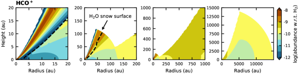
Figure 13: Abundance structure for HCO⁺ as shown in Fig. 4, but for model with a lower initial CO abundance of 10^-6.

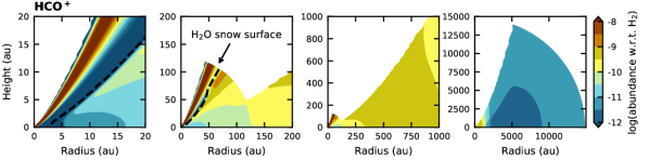
Figure 14: Abundance structure for HCO⁺ as shown in Fig. 4, but for model with a higher initial H₂O abundance of 10^-4.

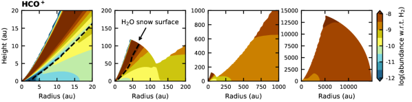
Figure 15: Abundance structure for HCO⁺ as shown in Fig. 4, but for model with a canonical cosmic ray ionization rate of $10^{-17}$ s^-1.

References

- ALMA Partnership et al. (2015) ALMA Partnership, Brogan, C. L., Pérez, L. M., et al. 2015, ApJ, 808, L3, doi: 10.1088/2041-8205/808/1/L3
- Andrews & Williams (2005) Andrews, S. M., & Williams, J. P. 2005, ApJ, 631, 1134, doi: 10.1086/432712
- Andrews et al. (2018) Andrews, S. M., Huang, J., Pérez, L. M., et al. 2018, ApJ, 869, L41, doi: 10.3847/2041-8213/aaf741
- Aso et al. (2017) Aso, Y., Ohashi, N., Aikawa, Y., et al. 2017, ApJ, 849, 56, doi: 10.3847/1538-4357/aa8264
- Balbus & Hawley (1991) Balbus, S. A., & Hawley, J. F. 1991, ApJ, 376, 214, doi: 10.1086/170270
- Bergin et al. (1998) Bergin, E. A., Melnick, G. J., & Neufeld, D. A. 1998, ApJ, 499, 777, doi: 10.1086/305656
- Bisschop et al. (2006) Bisschop, S. E., Fraser, H. J., Öberg, K. I., van Dishoeck, E. F., & Schlemmer, S. 2006, A&A, 449, 1297, doi: 10.1051/0004-6361:20054051
- Bosman et al. (2018) Bosman, A. D., Walsh, C., & van Dishoeck, E. F. 2018, A&A, 618, A182, doi: 10.1051/0004-6361/201833497
- Brinch & Hogerheijde (2010) Brinch, C., & Hogerheijde, M. R. 2010, A&A, 523, A25, doi: 10.1051/0004-6361/201015333
- Bryden et al. (1999) Bryden, G., Chen, X., Lin, D. N. C., Nelson, R. P., & Papaloizou, J. C. B. 1999, ApJ, 514, 344, doi: 10.1086/306917
- Cassen & Moosman (1981) Cassen, P., & Moosman, A. 1981, Icarus, 48, 353, doi: 10.1016/0019-1035(81)90051-8
- Cleeves et al. (2014) Cleeves, L. I., Bergin, E. A., & Adams, F. C. 2014, ApJ, 794, 123, doi: 10.1088/0004-637X/794/2/123
- Cleeves et al. (2015) Cleeves, L. I., Bergin, E. A., Qi, C., Adams, F. C., & Öberg, K. I. 2015, ApJ, 799, 204, doi: 10.1088/0004-637X/799/2/204
- Collings et al. (2003) Collings, M. P., Dever, J. W., Fraser, H. J., McCoustra, M. R. S., & Williams, D. A. 2003, ApJ, 583, 1058, doi: 10.1086/345389
- Davis (2005) Davis, S. S. 2005, ApJ, 620, 994, doi: 10.1086/427073
- Dong et al. (2018) Dong, R., Liu, S.-y., Eisner, J., et al. 2018, ApJ, 860, 124, doi: 10.3847/1538-4357/aac6cb
- Dra̧żkowska & Alibert (2017) Dra̧żkowska, J., & Alibert, Y. 2017, A&A, 608, A92, doi: 10.1051/0004-6361/201731491
- Du et al. (2017) Du, F., Bergin, E. A., Hogerheijde, M., et al. 2017, ApJ, 842, 98, doi: 10.3847/1538-4357/aa70ee
- Eistrup et al. (2016) Eistrup, C., Walsh, C., & van Dishoeck, E. F. 2016, A&A, 595, A83, doi: 10.1051/0004-6361/201628509
- Eistrup et al. (2018) —. 2018, A&A, 613, A14, doi: 10.1051/0004-6361/201731302
- Favre et al. (2017) Favre, C., López-Sepulcre, A., Ceccarelli, C., et al. 2017, A&A, 608, A82, doi: 10.1051/0004-6361/201630177
- Fraser et al. (2001) Fraser, H. J., Collings, M. P., McCoustra, M. R. S., & Williams, D. A. 2001, MNRAS, 327, 1165, doi: 10.1046/j.1365-8711.2001.04835.x
- Gaches & Offner (2018) Gaches, B. A. L., & Offner, S. S. R. 2018, ApJ, 861, 87, doi: 10.3847/1538-4357/aac94d
- Gaia Collaboration et al. (2021) Gaia Collaboration, Brown, A. G. A., Vallenari, A., et al. 2021, A&A, 649, A1, doi: 10.1051/0004-6361/202039657
- Gammie (1996) Gammie, C. F. 1996, ApJ, 457, 355, doi: 10.1086/176735
- Garaud & Lin (2007) Garaud, P., & Lin, D. N. C. 2007, ApJ, 654, 606, doi: 10.1086/509041
- Garrod & Herbst (2006) Garrod, R. T., & Herbst, E. 2006, A&A, 457, 927, doi: 10.1051/0004-6361:20065560
- Green et al. (2013) Green, J. D., Evans, Neal J., I., Jørgensen, J. K., et al. 2013, ApJ, 770, 123, doi: 10.1088/0004-637X/770/2/123
- Gressel et al. (2012) Gressel, O., Nelson, R. P., & Turner, N. J. 2012, MNRAS, 422, 1140, doi: 10.1111/j.1365-2966.2012.20701.x
- Güdel et al. (2007) Güdel, M., Briggs, K. R., Arzner, K., et al. 2007, A&A, 468, 353, doi: 10.1051/0004-6361:20065724
- Harsono et al. (2018) Harsono, D., Bjerkeli, P., van der Wiel, M. H. D., et al. 2018, Nature Astronomy, 2, 646, doi: 10.1038/s41550-018-0497-x
- Harsono et al. (2015) Harsono, D., Bruderer, S., & van Dishoeck, E. F. 2015, A&A, 582, A41, doi: 10.1051/0004-6361/201525966
- Harsono et al. (2020) Harsono, D., Persson, M. V., Ramos, A., et al. 2020, A&A, 636, A26, doi: 10.1051/0004-6361/201935994
- Hartmann et al. (1998) Hartmann, L., Calvet, N., Gullbring, E., & D’Alessio, P. 1998, ApJ, 495, 385, doi: 10.1086/305277
- Hsieh et al. (2019) Hsieh, T.-H., Murillo, N. M., Belloche, A., et al. 2019, ApJ, 884, 149, doi: 10.3847/1538-4357/ab425a
- Jørgensen et al. (2004) Jørgensen, J. K., Schöier, F. L., & van Dishoeck, E. F. 2004, A&A, 416, 603, doi: 10.1051/0004-6361:20034440
- Jørgensen et al. (2005) —. 2005, A&A, 435, 177, doi: 10.1051/0004-6361:20042092
- Jørgensen et al. (2013) Jørgensen, J. K., Visser, R., Sakai, N., et al. 2013, ApJ, 779, L22, doi: 10.1088/2041-8205/779/2/L22
- Karska et al. (2018) Karska, A., Kaufman, M. J., Kristensen, L. E., et al. 2018, ApJS, 235, 30, doi: 10.3847/1538-4365/aaaec5
- Kataoka et al. (2016) Kataoka, A., Muto, T., Momose, M., Tsukagoshi, T., & Dullemond, C. P. 2016, ApJ, 820, 54, doi: 10.3847/0004-637X/820/1/54
- Kataoka et al. (2015) Kataoka, A., Muto, T., Momose, M., et al. 2015, ApJ, 809, 78, doi: 10.1088/0004-637X/809/1/78
- Krolikowski et al. (2021) Krolikowski, D. M., Kraus, A. L., & Rizzuto, A. C. 2021, AJ, 162, 110, doi: 10.3847/1538-3881/ac0632
- Kruijer et al. (2017) Kruijer, T. S., Burkhardt, C., Budde, G., & Kleine, T. 2017, Proceedings of the National Academy of Science, 114, 6712, doi: 10.1073/pnas.1704461114
- Kwon et al. (2009) Kwon, W., Looney, L. W., Mundy, L. G., Chiang, H.-F., & Kemball, A. J. 2009, ApJ, 696, 841, doi: 10.1088/0004-637X/696/1/841
- Lecar et al. (2006) Lecar, M., Podolak, M., Sasselov, D., & Chiang, E. 2006, ApJ, 640, 1115, doi: 10.1086/500287
- Leemker et al. (2021) Leemker, M., van’t Hoff, M. L. R., Trapman, L., et al. 2021, A&A, 646, A3, doi: 10.1051/0004-6361/202039387
- Leya et al. (2008) Leya, I., Schönbächler, M., Wiechert, U., Krähenbühl, U., & Halliday, A. N. 2008, Earth and Planetary Science Letters, 266, 233, doi: 10.1016/j.epsl.2007.10.017
- Lichtenberg et al. (2021) Lichtenberg, T., Dra̧żkowska, J., Schönbächler, M., Golabek, G. J., & Hands, T. O. 2021, Science, 371, 365, doi: 10.1126/science.abb3091
- Mathews et al. (2013) Mathews, G. S., Klaassen, P. D., Juhász, A., et al. 2013, A&A, 557, A132, doi: 10.1051/0004-6361/201321600
- van ’t Hoff et al. (2017) van ’t Hoff, M. L. R., Walsh, C., Kama, M., Facchini, S., & van Dishoeck, E. F. 2017, A&A, 599, A101, doi: 10.1051/0004-6361/201629452
- McElroy et al. (2013) McElroy, D., Walsh, C., Markwick, A. J., et al. 2013, A&A, 550, A36, doi: 10.1051/0004-6361/201220465
- McMullin et al. (2007) McMullin, J. P., Waters, B., Schiebel, D., Young, W., & Golap, K. 2007, in Astronomical Society of the Pacific Conference Series, Vol. 376, Astronomical Data Analysis Software and Systems XVI, ed. R. A. Shaw, F. Hill, & D. J. Bell, 127
- Milam et al. (2005) Milam, S. N., Savage, C., Brewster, M. A., Ziurys, L. M., & Wyckoff, S. 2005, ApJ, 634, 1126, doi: 10.1086/497123
- Notsu et al. (2018) Notsu, S., Nomura, H., Walsh, C., et al. 2018, ApJ, 855, 62, doi: 10.3847/1538-4357/aaaa72
- Notsu et al. (2021) Notsu, S., van Dishoeck, E. F., Walsh, C., Bosman, A. D., & Nomura, H. 2021, A&A, 650, A180, doi: 10.1051/0004-6361/202140667
- Notsu et al. (2019) Notsu, S., Akiyama, E., Booth, A., et al. 2019, ApJ, 875, 96, doi: 10.3847/1538-4357/ab0ae9
- Öberg et al. (2011) Öberg, K. I., Murray-Clay, R., & Bergin, E. A. 2011, ApJ, 743, L16, doi: 10.1088/2041-8205/743/1/L16
- Ohashi et al. (1997) Ohashi, N., Hayashi, M., Ho, P. T. P., & Momose, M. 1997, ApJ, 475, 211, doi: 10.1086/303533
- Oka et al. (2011) Oka, A., Nakamoto, T., & Ida, S. 2011, ApJ, 738, 141, doi: 10.1088/0004-637X/738/2/141
- Oya et al. (2015) Oya, Y., Sakai, N., Lefloch, B., et al. 2015, ApJ, 812, 59, doi: 10.1088/0004-637X/812/1/59
- Padovani et al. (2015) Padovani, M., Hennebelle, P., Marcowith, A., & Ferrière, K. 2015, A&A, 582, L13, doi: 10.1051/0004-6361/201526874
- Padovani et al. (2018) Padovani, M., Ivlev, A. V., Galli, D., & Caselli, P. 2018, A&A, 614, A111, doi: 10.1051/0004-6361/201732202
- Padovani et al. (2016) Padovani, M., Marcowith, A., Hennebelle, P., & Ferrière, K. 2016, A&A, 590, A8, doi: 10.1051/0004-6361/201628221
- Phillips et al. (1992) Phillips, T. G., van Dishoeck, E. F., & Keene, J. 1992, ApJ, 399, 533, doi: 10.1086/171945
- Sakai et al. (2014) Sakai, N., Oya, Y., Sakai, T., et al. 2014, ApJ, 791, L38, doi: 10.1088/2041-8205/791/2/L38
- Schmalzl et al. (2014) Schmalzl, M., Visser, R., Walsh, C., et al. 2014, A&A, 572, A81, doi: 10.1051/0004-6361/201424236
- Schöier et al. (2005) Schöier, F. L., van der Tak, F. F. S., van Dishoeck, E. F., & Black, J. H. 2005, A&A, 432, 369, doi: 10.1051/0004-6361:20041729
- Schoonenberg & Ormel (2017) Schoonenberg, D., & Ormel, C. W. 2017, A&A, 602, A21, doi: 10.1051/0004-6361/201630013
- Schwarz et al. (2019) Schwarz, K. R., Bergin, E. A., Cleeves, L. I., et al. 2019, ApJ, 877, 131, doi: 10.3847/1538-4357/ab1c5e
- Segura-Cox et al. (2020) Segura-Cox, D. M., Schmiedeke, A., Pineda, J. E., et al. 2020, Nature, 586, 228, doi: 10.1038/s41586-020-2779-6
- Seifert et al. (2021) Seifert, R. A., Cleeves, L. I., Adams, F. C., & Li, Z.-Y. 2021, ApJ, 912, 136, doi: 10.3847/1538-4357/abf09a
- Sheehan et al. (2020) Sheehan, P. D., Tobin, J. J., Federman, S., Megeath, S. T., & Looney, L. W. 2020, ApJ, 902, 141, doi: 10.3847/1538-4357/abbad5
- Shirley et al. (2011) Shirley, Y. L., Mason, B. S., Mangum, J. G., et al. 2011, AJ, 141, 39, doi: 10.1088/0004-6256/141/2/39
- Stevenson & Lunine (1988) Stevenson, D. J., & Lunine, J. I. 1988, Icarus, 75, 146, doi: 10.1016/0019-1035(88)90133-9
- Tobin et al. (2008) Tobin, J. J., Hartmann, L., Calvet, N., & D’Alessio, P. 2008, ApJ, 679, 1364, doi: 10.1086/587683
- Tobin et al. (2012) Tobin, J. J., Hartmann, L., Chiang, H.-F., et al. 2012, Nature, 492, 83, doi: 10.1038/nature11610
- Tobin et al. (2013) —. 2013, ApJ, 771, 48, doi: 10.1088/0004-637X/771/1/48
- Trinquier et al. (2009) Trinquier, A., Elliott, T., Ulfbeck, D., et al. 2009, Science, 324, 374, doi: 10.1126/science.1168221
- Tsukamoto et al. (2021) Tsukamoto, Y., Machida, M. N., & Inutsuka, S.-i. 2021, ApJ, 920, L35, doi: 10.3847/2041-8213/ac2b2f
- Tychoniec et al. (2020) Tychoniec, Ł., Manara, C. F., Rosotti, G. P., et al. 2020, A&A, 640, A19, doi: 10.1051/0004-6361/202037851
- Ulrich (1976) Ulrich, R. K. 1976, ApJ, 210, 377, doi: 10.1086/154840
- Umebayashi & Nakano (1980) Umebayashi, T., & Nakano, T. 1980, PASJ, 32, 405
- Umebayashi & Nakano (1981) —. 1981, PASJ, 33, 617
- Umebayashi & Nakano (2009) —. 2009, ApJ, 690, 69, doi: 10.1088/0004-637X/690/1/69
- van der Tak et al. (2020) van der Tak, F. F. S., Lique, F., Faure, A., Black, J. H., & van Dishoeck, E. F. 2020, Atoms, 8, 15, doi: 10.3390/atoms8020015
- van ’t Hoff et al. (2018a) van ’t Hoff, M. L. R., Persson, M. V., Harsono, D., et al. 2018a, A&A, 613, A29, doi: 10.1051/0004-6361/201731656
- van ’t Hoff et al. (2018b) van ’t Hoff, M. L. R., Tobin, J. J., Harsono, D., & van Dishoeck, E. F. 2018b, A&A, 615, A83, doi: 10.1051/0004-6361/201732313
- van ’t Hoff et al. (2020) van ’t Hoff, M. L. R., Harsono, D., Tobin, J. J., et al. 2020, ApJ, 901, 166, doi: 10.3847/1538-4357/abb1a2
- van ’t Hoff et al. (2022) van ’t Hoff, M. L. R., Harsono, D., van Gelder, M. L., et al. 2022, ApJ, 924, 5, doi: 10.3847/1538-4357/ac3080
- Visser et al. (2012) Visser, R., Kristensen, L. E., Bruderer, S., et al. 2012, A&A, 537, A55, doi: 10.1051/0004-6361/201117109
- Whitney et al. (2003) Whitney, B. A., Wood, K., Bjorkman, J. E., & Wolff, M. J. 2003, ApJ, 591, 1049, doi: 10.1086/375415
- Yang et al. (2016) Yang, H., Li, Z.-Y., Looney, L. W., et al. 2016, MNRAS, 460, 4109, doi: 10.1093/mnras/stw1253
- Zhou et al. (1996) Zhou, S., Evans, Neal J., I., & Wang, Y. 1996, ApJ, 466, 296, doi: 10.1086/177510
- Zhu et al. (2014) Zhu, Z., Stone, J. M., Rafikov, R. R., & Bai, X.-n. 2014, ApJ, 785, 122, doi: 10.1088/0004-637X/785/2/122