Self-Supervised Equivariant Learning for Oriented Keypoint Detection

Abstract

Detecting robust keypoints from an image is an integral part of many computer vision problems, and the characteristic orientation and scale of keypoints play an important role for keypoint description and matching. Existing learning-based methods for keypoint detection rely on standard translation-equivariant CNNs but often fail to detect reliable keypoints against geometric variations. To learn to detect robust oriented keypoints, we introduce a self-supervised learning framework using rotation-equivariant CNNs. We propose a dense orientation alignment loss by an image pair generated by synthetic transformations for training a histogram-based orientation map. Our method outperforms the previous methods on an image matching benchmark and a camera pose estimation benchmark.

1 Introduction

Detecting robust keypoints is an integral part of many computer vision tasks, such as image matching [21], visual localization [54, 55, 28], SLAM [39, 13, 14], and 3D reconstruction [57, 1, 19, 77]. The robust keypoints, in principle, are consistently localizable, being invariant to photometric/geometric variations of an image induced by viewpoint/illumination changes, and a keypoint is typically assigned with its characteristic orientation/scale as a geometric feature, which plays an important role for keypoint description [27, 51, 37, 45, 62, 63, 15, 14, 71, 41] or matching [72, 74, 6, 53], as shown in Fig. 1. As rotation frequently occurs for patterns of interests in real-world images, the keypoints and their geometric features are required to be consistent w.r.t rotation of the image in particular.

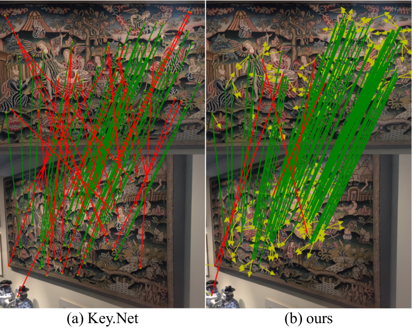
Figure 1: Visualization of the predicted matches to compare the existing keypoint detector Key.Net [3] (left) with our oriented keypoint detector (right). We draw the correct matches (green) and the incorrect matches (red) using the ground-truth homography. We extract 300 keypoints and use HardNet [37] descriptor for matching. The arrows of the keypoints in the right denote the estimated orientations which are used for filtering outliers.

The early methods have detected keypoints with their charateristic orientation/scale using a hand-crafted filter on a shallow gradient-based feature map. For example, SIFT [27] detects the keypoints by finding local extrema in difference-of-Gaussian (DoG) features on a scale space and obtains a dominant orientation from gradient histograms. While such a technique has proven effective for shallow gradient-based feature maps, it cannot be applied to deep feature maps from standard networks, where rotation or scaling induces unpredictable variations of features. Recent methods [71, 41, 58, 3], thus, rely on learning from data. They typically train a convolutional neural network (CNN) for keypoint detection and/or description by regressing orientation and scale. Some [41, 3] adopt self-supervised learning through synthetic transformation, while others [58, 71] train the networks through strong supervision by homography or SfM. All these approaches, however, often fail to detect reliable keypoints against geometric variations; they learn invariance or equivariance by relying on training with data augmentation, which does not provide a sufficient level for keypoint detection.

In this work, we propose a self-supervised equivariant learning method for oriented keypoint detection. Recent studies [10, 29, 76, 68, 69, 11] introduce different equivariant neural networks that embed an explicit structure for equivariant learning by design. The group-equivariant CNNs on a cyclic group have the advantages of explicitly encoding the enriched orientation information and reducing the number of model parameters through weight sharing compared to the conventional CNNs. We propose an orientation alignment loss to estimate a characteristic orientation to the keypoint using a histogram-based representation. The histogram-based representation provides richer information than the regression methods [73, 41, 71] by predicting multiple candidates for the orientations. To train the invariant keypoint detector, we utilize a window-based loss [3] to satisfy the geometric consistency with anchor points diverse across the image. We generate the synthetic image pairs by a random in-plane rotation to create diverse examples and reduce the annotation cost. In addition, we generate a scale-space representation in the networks and use multi-scale inference to consider scale-invariance approximately.

We evaluate the rotation-invariant keypoint detection and the rotation-equivariant orientation estimation compared under synthetic rotations with the existing models [27, 51, 41]. We validate the effectiveness of our keypoint detector compared to the handcrafted methods [27, 51] and the learning-based methods [14, 15, 45, 3] in an image matching benchmark [2] using a repeatability score and matching accuracy. The estimated orientations improve the image matching accuracy with an outlier filtering in HPatches [2]. Furthermore, we show the transferability to a more complex task by evaluating 6 DoF pose estimation in IMC2021 [21]. We demonstrate ablation experiments and visualizations to verify the effectiveness of our model.

The contributions of our paper are three-fold:

• We propose a self-supervised framework for learning to detect rotation-invariant keypoints using a rotation-equivariant representation.

• We propose a dense orientation alignment loss by aligning a pair of histogram tensors to train the characteristic orientations.

• We demonstrate the effectiveness of our oriented keypoint detector with extensive evaluations compared to existing keypoint detection methods on standard image matching benchmarks.

2 Related work

Keypoint detection for image matching. Traditional keypoint detectors rely on carefully designed handcrafted filters. Harris [18] and Hessian [5] use first and second order image derivatives to find corners or blobs in images. Those detectors are extended by handling multi-scale and affine transformations [32, 34]. SIFT [27] detect keypoints by finding local extrema from the DoG features, and SURF [4] further boost up speed by using the Haar filters. ORB [51] propose a oriented FAST [50] detector. Recently, learning-based methods [66, 71, 14, 41, 58, 15, 45, 61, 56, 65, 40] use a CNN-based response map to train a keypoint detector. Key.Net [3] utilize the benefit of both representation of the handcrafted and the learning-based to improve the performance in terms of repeatability. Also, some methods [8, 48, 35, 36, 47, 64, 24] find correspondences in a correlation tensor using a pair of dense features without a separate keypoint detector, but constructing the correlation tensor requires high memory consumption, so it compromises the pixel accuracy of correspondences. Contrary to the learning methods that use a conventional translation-equivariant CNN, we utilize a rotation-equivariant CNN to obtain consistent 2D keypoints. Our model can significantly reduce the number of model parameters by weight sharing in group convolution.

Local orientation estimation. SIFT [27] use a histogram of image gradients to estimate the local orientation. ORB [51] propose an efficient way to measure corner orientation using intensity centroid [49]. Learning-based methods learn the orientation implicitly through a descriptor similarity loss [73, 38, 58, 16] or explicitly through an orientation regression loss [71, 41], and they use the orientation as one of the affine parameters in patch sampling using STNs [20]. While [71, 41] learns sparse orientations of keypoints using the regression loss that minimizes the distance of angles, our model learns dense orientations of all positions using the histogram alignment loss that matches the shifted orientation histograms. Compared to regression of [71, 41], our histogram output naturally facilitates the prediction of multiple orientations and the loss of histogram alignment with the rotation-equivariant representations allows more robust learning. A previous work [23] proposes the histogram alignment loss at the local patch-level, but we extend it to all the regions of an image. The orientations are verified through an outlier filtering for image matching.

Equivariant representation learning. [31, 30, 59] propose an equivariant representation based on restricted Boltzmann machines (RBM) through tensor factorization. Since CNNs became popular, [10] proposes group equivariant convolutional networks using discrete isometric groups. [29, 76] propose resampling filters using interpolation to encode explicit orientations. [68, 69] use harmonics as filters to extract equivariant features from more diverse groups and continuous domains. [67] extend this group to the general $E(2)$ groups, and [60] propose scale-equivariant steerable networks. From an application point of view, [17] propose rotation-equivariant networks to solve the rotated object detection on the aerial images. [44] apply the equivariant CNN for registration of multimodal images. [43] disentangle the invariance group of illumination and viewpoint for training local descriptors. The most similar work, GIFT [26], use equivariant networks to obtain dense local descriptors, but [26] constructs the group representation with augmented images, whereas we construct the representation through steerable kernels [67] without rotating images at runtime.

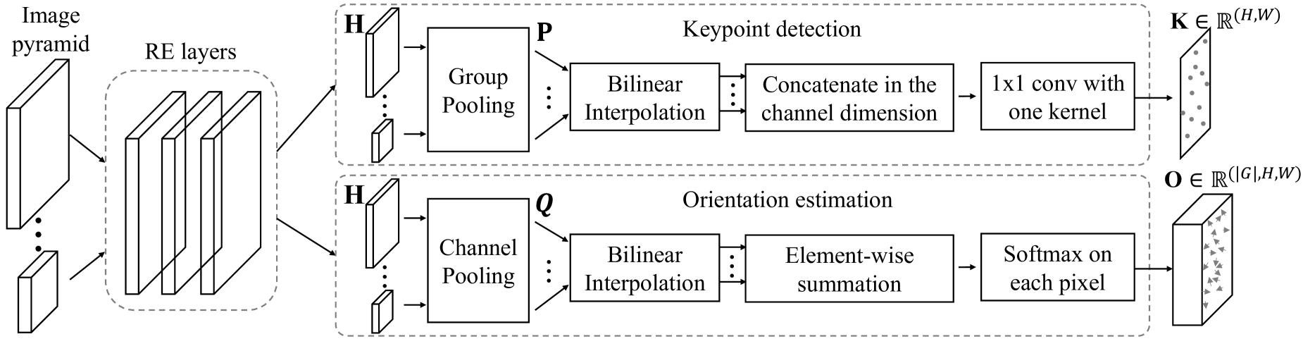
Figure 2: Overall architecture. The rotation-equivariant convolutional layer takes an input image and processes it at multiple scales. The multi-scale rotation-equivariant representation $\mathbf{H}$s pass two separate branches that predict a keypoint map $\mathbf{K}$ and an orientation map $\mathbf{O}$.

3 Rotation-equivariant keypoint detection

3.1 Overview

The goal of our work is to learn to detect oriented keypoints from images. The classical keypoint detectors relying on handcrafted features satisfy the rotation/translation equivariance, but the handcrafted methods are sensitive to illumination changes or color distortions. On the contrary, recent learning-based keypoint detectors use standard CNNs to encode local geometry and high-level semantics through convolutional layers. The convolution operation is inherently translation-equivariant, not rotation-equivariant. Therefore, we use a rotation-equivariant convolution [67] without handcrafted features to take advantages of both approaches. The rotation-equivariant CNN features contribute to extract rotation-invariant keypoints with the orientations.

Figure 2 shows the proposed method which consists of rotation-equivariant layers and is followed by two branches, the keypoint detection and the orientation estimation. The keypoint detection branch generates a rotation-invariant keypoint score map through group pooling and the orientation estimation branch generates a rotation-preserving orientation map through channel pooling. A window-based keypoint detection loss [3] and the proposed dense orientation alignment loss are used to learn the oriented keypoints in a self-supervised manner. Furthermore, the multi-scale image pyramid encourages the network to have robustness to scale changes.

3.2 Preliminaries

Equivariance. A feature extractor $\Phi$ is said to be equivariant to a geometric transformation $T_{g}$ if transforming an input $x\in X$ by the transformation $T_{g}$ and then passing it through the feature extractor $\Phi$ gives the same result as first mapping $x$ through $\Phi$ and then transforming the feature map by $T^{\prime}_{g}$ [67]. Formally, the equivariance can be expressed for transformation group $G$ and $\Phi:X\rightarrow Y$ as

$$\Phi[T_{g}(x)]=T^{\prime}_{g}[\Phi(x)],$$ (1)

where $T_{g}$ and $T^{\prime}_{g}$ represent transformations on each space as a predefined group action $g\in G$. In this case, the function $\Phi$ operates a “structure-preserving” mapping from one representation to another. For example, convolutional operation is designed to be translation-equivariant. If $T_{t}$ is a translation group $(\mathbb{R}^{2},+)$, and $f$ is the $K$-dimension feature mapping sent to $\mathbb{Z}^{2}\rightarrow\mathbb{R}^{K}$, the translation equivariance can be expressed as follows:

$$[T_{t}f]*\psi(x)=[T_{t}[f*\psi]](x),$$ (2)

where $\psi$ denotes convolution filter weights $\mathbb{Z}^{2}\rightarrow\mathbb{R}^{K}$, and $*$ indicates the convolution operation.

Group-equivariant convolution. Recent studies [67, 11, 68, 10, 12] have developed convolutional neural networks that are equivariant to symmetry groups of translation, rotation and reflection. Let $H$ be a rotation group. The group $G$ can be defined by $G\cong(\mathbb{R}^{2},+)\rtimes H$ as the semidirect product of the translation group $(\mathbb{R}^{2},+)$ with the rotation group $H$. Then, the rotation-equivariant convolution on group $G$ can be defined as:

$$[T_{g}f]*\psi(g)=[T_{g}[f*\psi]](g),$$ (3)

by replacing $t\in(\mathbb{R}^{2},+)$ with $g\in G$ in Eq. 2. This operation can apply to an input tensor to produce a translation and rotation-equivariant output. Note that the cyclic group $G_{N}$ represents an interval of $\frac{2\pi}{N}$ representing discrete rotations.

A rotation-equivariant network can be constructed by stacking rotation-equivariant layers similar to standard CNNs. This network becomes equivariant to both translation and rotation in the same way with the translation-equivariant convolutional networks. Formally, let $\Phi=\{L_{i}|i\in\{1,2,3,...,M\}\}$, which consists of $M$ rotation-equivariant layers under group $G$. For one layer $L_{i}\in\Phi$, the transformation $T_{g}$ is defined as

$$L_{i}[T_{g}(g)]=T_{g}[L_{i}(g)],$$ (4)

which indicates that the output is preserved after $L_{i}$ about $T_{g}$. Extending this, if we apply $T_{g}$ to input $I$ and then pass it through the network $\phi$, the transformation $T_{g}$ is preserved for the whole network.

$$[\Pi_{i=1}^{M}L_{i}](T_{g}I)=T_{g}[\Pi_{i=1}^{M}L_{i}](I).$$ (5)

3.3 Oriented keypoint detection networks

In this subsection, we describe the process of creating representations for the rotation-invariant keypoint detection and the rotation-equivariant orientation estimation.

Rotation-equivariant feature extraction. For feature extraction, we use the rotation-equivariant convolutional layers using [67]. For computational efficiency in a limited computational resource, we consider a discrete rotation group only. The layer acts on $(\mathbb{R}^{2},+)\rtimes G_{N}$ and is equivariant for all translations and $N$ discrete rotations. At the first layer $L_{1}$, the scalar field of the input image is lifted to the vector field of the group representation by defining field types in a predefined group [67]. Given an input image, $M$ stacked layers produce an output feature map via

$$\mathbf{H}=[\Pi_{i=1}^{M}L_{i}](I),$$ (6)

where $\mathbf{H}\in\mathbb{R}^{|G|\times C\times H\times W}$ is a rotation-equivariant representation output, and $C$ is the number of channels assigned for each group action. In our experiments, we use 3 layers ($M=3$). The output $\mathbf{H}\in\mathbb{R}^{|G|\times C\times H\times W}$ is a group of feature maps, which represents $C$-channel feature maps for $|G|$ orientations, and $\mathbf{H}_{i}$ denotes a feature map for $i$-th orientation in $G$. This rotation-equivariant network enables an extensive sharing of kernel weights for different orientations, i.e., rotation transformations, and thus increasing sample efficiency in learning, particularly a rotation-involving task.

Rotation-invariant keypoint detection. Robust keypoints need to be invariant to rotation transformations; the keypointness, i.e., keypoint score, for a specific position on an image should not be affected by rotating the image. To obtain such a rotation-invariant map for keypoint scores, we collapse the group $G$ of $\mathbf{H}\in\mathbb{R}^{|G|\times C\times H\times W}$ by group pooling, reducing it to a rotation-invariant representation $\mathbf{P}\in\mathbb{R}^{C\times H\times W}$. Specifically, we use max pooling over orientations: $\mathbf{P}=\max_{g}\mathbf{H}_{g,:,:,:}$. Given multi-scale outputs $\{\mathbf{P}_{s}\}_{s\in S}$, the final score map $\mathbf{K}\in\mathbb{R}^{H\times W}$ is obtained using standard convolution $\rho$ over a concatenation of $\mathbf{P}_{s}$:

$$\mathbf{K}=\rho(\bigcup_{s\in S}(\zeta(\mathbf{P}_{s}))),$$ (7)

where $\rho$ is a convolution operation, $\bigcup$ means concatenation of the elements, and $\zeta$ denotes a bilinear interpolation function. The interpolation function resizes the input map to a target size, and the convolution transforms a rotation-invariant feature map to a rotation-invariant score map.

Rotation-equivariant orientation estimation. To estimate a characteristic orientation for a candidate keypoint, we leverage the orientation group of rotation-equivariant tensor $\mathbf{H}$ and translate it to the orientation histogram tensor $\mathbf{Q}$. Specifically, we collapse the channel dimension $C$ for each orientation by channel pooling and produce a $|G|$-channel feature map $\mathbf{Q}\in\mathbb{R}^{|G|\times H\times W}$, where each position can be seen as being assigned an orientation histogram of $|G|$ bins. We use the implementation with $1\times 1$ group convolution with a single filter to collapse the channels of each orientation:

$$\mathbf{Q}=\eta(\mathbf{H}_{:,c}),$$ (8)

where $\eta:\mathbb{R}^{|G|\times C}\rightarrow\mathbb{R}^{|G|}$ maps $\mathbf{H}$ to a discrete histogram distribution of $|G|$ bins. Note that the channel pooling can be any other operations, e.g., max pooling, average pooling, and so on. The resultant output can be interpreted as a map of characteristic orientations for corresponding positions. The output pixel-level rotation-equivariant representation $\mathbf{Q}$ is used to learn the keypoint orientation as a histogram-based dense probability map. Given multi-scale outputs $\{\mathbf{Q}_{s}\}_{s\in S}$, the final orientation probability tensor $\mathbf{O}\in\mathbb{R}^{|G|\times H\times W}$ is obtained by summing the outputs over the multiple scales.

$$\mathbf{O}=\sigma(\bigoplus_{s\in S}(\zeta(\mathbf{Q}_{s}))),$$ (9)

where $\sigma\in\mathbb{R}^{|G|}\rightarrow[0,1]^{|G|}$ is a softmax function, and $\bigoplus$ is element-wise summation operation.

3.4 Training

In this subsection, we describe two loss functions for the keypoint detection and the orientation estimation. First, the loss for the orientation estimation will be described.

Dense orientation alignment loss. We train the histogram tensor O to represent the orientations of each pixel. Our method takes both advantages of the histogram-based [27, 51] and the learning-based [73, 71, 41] approaches. The dense orientation tensor $\mathbf{O}\in\mathbb{R}^{|G|\times H\times W}$ encodes relative orientations for each feature point. We transform the histogram of the feature points in $\textbf{O}^{\mathrm{a}}$ and the spatial dimension of $\textbf{O}^{\mathrm{b}}$ to learn a characteristic orientation by an explicit supervision as illustrated in Figure 3.

Image pair $I^{\mathrm{a}}$, $I^{\mathrm{b}}$, and the known ground-truth rotation $T_{g}$ are assumed as the input of the networks. First, we rotate $\mathbf{O}^{\mathrm{b}}$ with $T_{g}^{-1}$ for spatial alignment. Next, a histogram alignment is performed by shifting the histograms of each position in $\mathbf{O}^{\mathrm{a}}$ using $T^{\prime}_{g}$ in vector space. Note that the histograms in each pixel of O are in a cyclic group $G$. Finally, the aligned representations $T^{\prime}_{g}(\mathbf{O}^{\mathrm{a}})$ and $T_{g}^{-1}(\mathbf{O}^{\mathrm{b}})$ are trained with the following cross-entropy loss for all pixels:

$$\mathcal{L}^{\mathrm{ori}}=-\sum_{i=1}^{W}\sum_{j=1}^{H}\mathbf{M}\cdot\sum_{k=1}^{|G|}T^{\prime}_{g}(\mathbf{O}^{\mathrm{a}})_{k}\log(T_{g}^{-1}(\mathbf{O}^{\mathrm{b}}))_{k},$$ (10)

where $\mathbf{M}=\bm{1}\wedge T_{g}^{-1}(\bm{1})$ is a mask for removing out-of-bound regions, and $\bm{1}\in{1}^{H\times W}$. We omit the spatial index $i,j$ of the tensors $\mathbf{O}^{\mathrm{a}}$, $\mathbf{O}^{\mathrm{b}}$ and $\mathbf{M}$ in Eq. 10 for simplicity.

Window-based keypoint detection loss. We utilize a keypoint detection loss using a multi-scale index proposal [3]. In general, a good keypoint is localized in a consistent location invariant to geometric or photometric image transformations. The window-based keypoint detection loss [3] takes both advantages of selecting anchor-based keypoints [14, 66, 75] and using homography without constraining their locations [25, 41].

The keypoint score map $\mathbf{K}\in\mathbb{R}^{H\times W}$ is transformed by non-maximum suppression through exponential scaling based on a window. A window $m^{(i)}$ in the score map K is derived by the softmax over the spatial window of size $N\times N$ around an image coordinate $(u,v)$:

$$~{}m^{(i)}_{u,v}=\frac{e^{w^{(i)}_{u,v}}}{\sum_{j=c^{(i)}}^{c^{(i)}+N}\sum_{k=c^{(i)}}^{c^{(i)}+N}e^{w^{(i)}_{j,k}}},$$ (11)

where a window $w^{(i)}$ is a nonoverlapping $i$-th $N\times N$ grid in the score map $\mathbf{K}$ and $c^{(i)}$ is the top-left coordinates of the window $w^{(i)}$. Then the maximum value in $m^{(i)}$ becomes the dominant location in the window, and a weighted average by multiplying the index in the window $w^{(i)}$ is performed as follows:

$$~{}[x^{(i)},y^{(i)}]^{\top}=[\bar{u}^{(i)},\bar{v}^{(i)}]^{\top}=\sum_{[u,v]\in w^{(i)}}m^{(i)}_{u,v}\cdot[u,v]^{\top},$$ (12)

where $[x^{(i)},y^{(i)}]^{\top}$ is a soft-selected coordinate in an image. Eqs.11-12 aim to suppress noisy predictions in selecting real-value coordinates of the keypoints and to make the layer differentiable, same to the soft-argmax used in [71].

The index proposal loss compares the soft-selected index with a hard-selected coordinate $[\hat{x}^{(i)},\hat{y}^{(i)}]$ obtained by $\operatorname*{arg\,max}$ in $w^{(i)}$ using the ground-truth geometric transformation $T_{g}$:

$$\mathcal{L}^{\mathrm{IP}} (I^{\mathrm{a}},I^{\mathrm{b}},T_{g},N)=$$ (13)

$$\sum_{i}\alpha^{(i)}||{[x^{(i)},y^{(i)}]^{\mathrm{a}}}^{\top}-T_{g}^{-1}{[\hat{x}^{(i)},\hat{y}^{(i)}]^{\mathrm{b}}}^{\top}||^{2},$$

$$\text{and }\alpha^{(i)}=\mathcal{R}^{\mathrm{a}}[x^{(i)},y^{(i)}]^{\mathrm{a}}+\mathcal{R}^{\mathrm{b}}[\hat{x}^{(i)},\hat{y}^{(i)}]^{\mathrm{b}},$$

where $\alpha^{(i)}$ is a weighting term based on the score maps, and $\mathcal{R}^{\mathrm{a}}$ and $\mathcal{R}^{\mathrm{b}}$ are the response map of $I^{\mathrm{a}}$ and $I^{\mathrm{b}}$ with coordinates related by $T_{g}^{-1}$. Finally, the keypoint detection loss uses multiple sizes of the window and adds switching term of the input source and target:

$$\mathcal{L}^{\mathrm{kpts}}(I^{\mathrm{a}},I^{\mathrm{b}},T_{g}) =\sum_{l}\lambda_{l}(\mathcal{L}^{\mathrm{IP}}(I^{\mathrm{a}},I^{\mathrm{b}},T_{g},N_{l})$$ (14)

$$+\mathcal{L}^{\mathrm{IP}}(I^{\mathrm{b}},I^{\mathrm{a}},T_{g}^{-1},N_{l})),$$

where $l$ is the index of a window level, $N_{l}$ is the window size in $l$, $\lambda_{l}$ is a balancing parameter at a window level.

We use the final loss function $\mathcal{L}$ as follows:

$$\mathcal{L}=\beta\mathcal{L}^{\mathrm{ori}}+\mathcal{L}^{\mathrm{kpts}},$$ (15)

where $\beta$ is a balancing parameter of the loss functions. Since image variations, in general, are not limited to discrete rotation but also include other geometric/photometric variations, e.g., continuous rotation, scaling, and illumination changes, $\mathcal{L}^{\mathrm{ori}}$ and $\mathcal{L}^{\mathrm{kpts}}$ are used to consider such variations in training. Both of the losses are thus non-zero despite our equivariant representation of the cyclic group $G_{N}$.

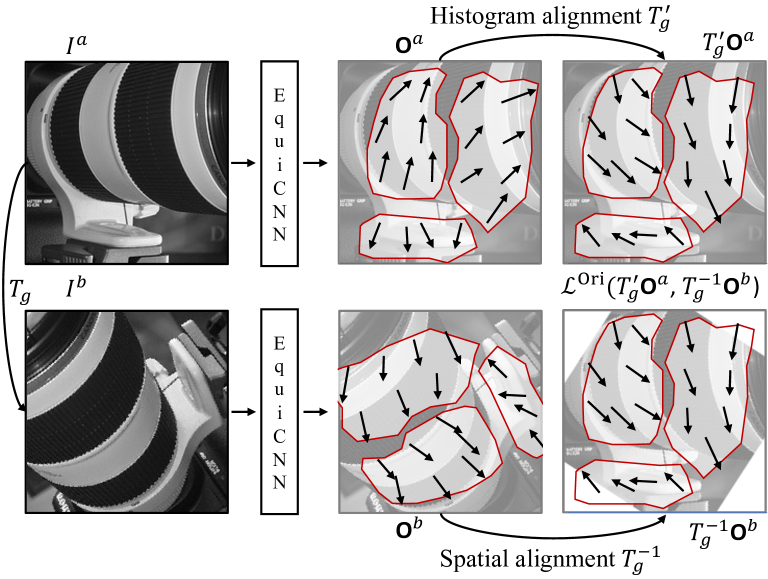
Figure 3: Illustration of dense orientation alignment loss. The dense orientation histogram $\mathbf{O}^{\mathrm{b}}$ is spatially aligned using $T^{-1}_{g}$. The equivariant histogram vectors of the feature points in $\mathbf{O}^{\mathrm{a}}$ are shifted using $T^{\prime}_{g}$. The out-of-plane regions are excluded when computing the loss.

4 Experiments

This section shows comparative experiments to demonstrate the effectiveness of our model. We describe the implementation details and the experimental benchmarks (Sec. 4.1). We experiment with the keypoints and the orientations under synthetic rotations (Sec. 4.2), and then show the results of keypoint matching on HPatches [2] and IMC2021 [21] (Sec. 4.3). We experiment the variations of our model and show the qualitative results (Sec. 4.4).

4.1 Experimental setting

Implementation details. We use the $E(2)$-CNN framework [67] for the implementation of rotation-equivariant convolution with PyTorch [42, 46]. We use 36 for the order of cyclic group $G$, with 2 for the channel dimension $C$. We use 3 equivariant layers, each of which consists of a conv-bn-relu module. Each convolution layer has $5\times 5$ kernel with padding of 2 without bias, and model parameters are randomly initialized. We use a batch size of 16. We train with Adam optimizer with a learning rate of 0.001. The leaning rate decay is 0.5 every 10 epochs for a total of 20 epochs. Early stopping is required to avoid overfitting, so we use the repeatability score of the validation set. The keypoint loss uses the window sizes $N_{l}\in[8,16,24,32,40]$ with $\lambda_{l}\in[256,64,16,4,1]$ same as [3], and the loss balancing parameter $\beta$ is 100. We use the NMS size $15\times 15$ at test time, same to Key.Net [3].

Inference. For robustness to the scale change, we make eight scale pyramids by the scaling of $\sqrt{2}$ at inference time. We extract $\lfloor\frac{2^{2-s}*\textbf{p}}{\sum_{n=-2}^{5}2^{n}}\rfloor$ keypoints at scale $s\in S=\{0,1,..,7\}$ when we extract a total of p keypoints. We assign the scale value $\sqrt{2}^{s-2}$ for the keypoints extracted in scale $s$. We use simple $\operatorname*{arg\,max}$ to obtain an orientation value from the histogram, which performs well enough compared to a soft prediction for deriving real value.

Training dataset. We generate a synthetic dataset for the self-supervised training. Our model needs a ground-truth relative orientation for the training. We generate random image pairs with in-plane rotation [-180, 180], which is sufficient for the planar homography [2] or the 3D viewpoint changes [21]. To improve the robustness at illumination changes, we modify the contrast, brightness, and hue value in HSV space. We exclude the images with insufficient edges through Sobel filters [22] as a pre-processing. The synthetic dataset has 9,100 image pairs of size $192\times 192$ split into 9,000 as a training set and 100 as a validation set. We use ILSVRC2012 [52] as source data.

Evaluation benchmark. We use two test datasets for comparative evaluation. HPatches [2] is for evaluating keypoint detection and matching. IMC2021 [21] is for evaluating the 6 DoF pose estimation accuracy.

HPatches consists of 116 scenes with 59 viewpoint variation and 57 illumination variation [2]. Each scene consists of 5 image pairs with ground-truth planar homography, for a total of 696 image pairs. We compare our model with the existing models using 1,000 keypoints for evaluation. We use the repeatability score, the number of matches, and mean matching accuracy (MMA) as evaluation metrics proposed to [15, 33]. Repeatability is the ratio between the number of repeatable keypoints and the total number of detections by 3 pixel threshold. MMA is the average percentage of correct matches per image pair. We measure the correct matches by thresholding 3 and 5 pixels for MMA.

IMC2021 is a large-scale challenge dataset of wide-baseline matching [21]. IMC2021 consists of an unconstrained urban scene with large illumination and viewpoint variations. In this experiment, we compare our method with the existing keypoint detection methods in an image matching pipeline [37, 7, 9]. We experiment on the stereo track using the validation sets of Phototourism and PragueParks. This benchmark takes the predicted matches as an input and measures the 6 DoF pose estimation accuracy. We measure the mean average accuracy (mAA) of pose estimation at 5°and 10°and the number of inliers.

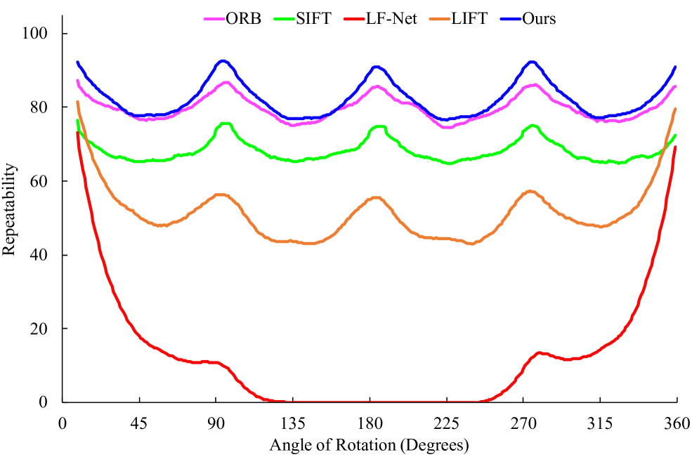
Figure 4: Results of repeatability to evaluate the rotation-invariant keypoint detection under synthetic rotations with Gaussian noise. For a better view, we smooth the chart by a moving average.

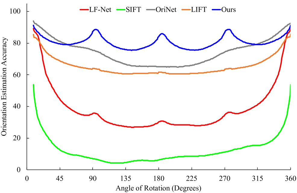
Figure 5: Results of orientation estimation accuracy under synthetic rotations with Gaussian noise. We use $15\degree$ threshold for measuring the accuracy.

4.2 Experiments under synthetic rotations

Inspired by Section 4.4 of [51], we conduct two experiments with synthetic images using in-plane rotation from $0\degree$ to $359\degree$ at $1\degree$ intervals using ten images of size $224\times 224$ that are not used for training and validation. We compare two handcrafted methods [27, 51] and two learning methods [41, 71] among the representative keypoint detectors that yield the orientations. Figure 4 shows the results of rotation-invariant keypoint detection in terms of repeatability. Our method consistently obtains better repeatability than the existing methods [27, 51, 41, 71]. Note that the learning method LF-Net [41] falls off dramatically after 10 degrees while the handcrafted, SIFT [27] and ORB [51], are robust to rotations. Figure 5 shows the results of rotation-equivariant orientation estimation in terms of orientation estimation accuracy. We align $\textbf{O}^{\mathrm{b}}$ to $\textbf{O}^{\mathrm{a}}$ using $T^{-1}_{g}$ and then measure the accuracy at the whole region of images except the boundary regions as in Figure 6. We obtain the orientation values of SIFT [27] by generating keypoints in all positions. Even though our method predicts the orientation discretely by the histogram, it is more effective than the regression-based learning methods, OriNet [73], LIFT [71], and LF-Net [41]. Especially, the accuracies of our model are consistently over 80% at a threshold of 15 degrees.

4.3 Keypoint matching

		All variations
Det.	Desc.	Rep.	MMA		pred. match.
			@3px	@5px
SIFT [27]	SIFT [27]	41.9	49.4	52.4	404.2
SIFT [27]	HardNet [37]	41.9	57.1	62.3	437.8
SIFT [27]	SOSNet [63]	41.9	57.9	63.0	430.8
SIFT [27]	HyNet [62]	41.9	57.3	62.5	438.9
ORB [51]	ORB [51]	57.4	46.6	50.0	362.0
D2-Net [15]	D2-Net [15]	19.8	35.2	48.6	371.8
LF-Net [41]	LF-Net [41]	43.8	52.0	56.9	330.2
R2D2 [45]	R2D2 [45]	45.5	64.6	74.8	358.9
SPoint [14]	SPoint [14]	47.0	63.9	70.3	466.3
SPoint [14]	GIFT [26]	47.0	68.8	76.0	496.7
Key.Net [3]	HardNet [37]	55.9	72.5	79.4	474.4
Key.Net [3]	SOSNet [63]	55.9	72.7	79.6	464.7
Key.Net [3]	HyNet [62]	55.9	72.0	78.9	475.3
ours	HardNet [37]	57.6	73.1	79.6	505.8
ours	SOSNet [63]	57.6	73.4	80.0	499.5
ours	HyNet [62]	57.6	72.9	79.5	503.3
ours	GIFT [26]	57.6	75.2	81.5	415.6

Table 1: Results on HPatches. We use 1,000 keypoints in this experiment. ‘Det.’ denotes keypoint detection method, ‘Desc.’ denotes descriptor extraction method, ‘Rep.’ denotes the repeatability score, and ‘pred. match.’ is the average number of predicted matches. Numbers in bold indicate the best scores.

Results on HPatches. Table 1 shows the results of keypoint detection and matching in HPatches [2]. We exclude our orientation in this experiment. We compare the handcrafted detectors [27, 51] and a learned detector [3] as baselines with patch-based descriptors [37, 63, 62]. We additionally compare the joint detection and description methods [15, 45, 41, 14] and the integration of the rotation-invariant dense descriptors [26]. We use the mutual nearest neighbor matching algorithm for all cases in this experiment. Our model achieves the best repeatability score compared to the existing keypoint detection methods [27, 51, 15, 45, 41, 14, 3], which means our detector is robust to the viewpoint and illumination changes. Our model consistently obtains more predicted matches and better MMA scores compared to the state-of-the-art keypoint detector Key.Net [3] at all cases with the patch descriptors [37, 63, 62]. Our model with GIFT descriptor [26] achieves better MMAs compared to the SuperPoint [14] detector of the cases with SuperPoint descriptor [14] and GIFT [26]. In particular, our model with the rotation-invariant descriptors [26] achieves the best MMAs, which shows that the rotation-invariant representation contributes to improving the accuracy of correspondences.

Det.	K	Stereo track.
		Num. Inl.	mAA(5°)	mAA(10°)
DoG+AN [27, 38]	1,024	43.8	0.210	0.277
Key.Net [3]	1,024	126.5	0.397	0.512
ours	1,024	135.6	0.441	0.549
DoG+AN [27, 38]	2,048	105.9	0.385	0.477
Key.Net [3]	2,048	245.4	0.473	0.588
ours	2,048	269.3	0.521	0.632
DoG+AN [27, 38]	8,000	539.0	0.605	0.718
Key.Net [3]	8,000	563.0	0.522	0.635
ours	8,000	992.9	0.601	0.710

Table 2: Mean average accuracy (mAA; 5°, 10°) of 6-DoF pose estimation and the average number of inlier matches (Num. Inl.) on IMC2021 validation set [21]. Column ‘K’ denotes the number of keypoints. Numbers in bold indicate the best scores.

Results on the IMC2021. Table 2 shows the results of 6 DoF pose estimation in IMC2021 [21] for evaluating on a complex task of general scenes. For this experiment, we use the rest of the image matching pipeline using HardNet descriptor [37], and DEGENSAC geometric verification [9] with AdaLAM [7] for all cases. For the AdaLAM [7] stage, we use our estimated orientation values and the scale values from the scale-space inference. We compare to two baselines, DoG+AN [27, 38] and Key.Net [3]. The result shows that our model consistently improves the camera pose estimation accuracy (mAAs) and the number of inliers compared to the Key.Net [3]. Although the mAAs of our model in 8,000 keypoints are slightly lower than DoG+AN [27, 38], the number of inliers is almost double which denotes the quality of 3D reconstruction. In particular, our model with 1,024 keypoints significantly improves the mAAs and the number of inliers compared to DoG+AN [27, 38], which shows that our model estimates more accurate camera poses with less computation. Our model consistently outperforms the baseline Key.Net [3] for all metrics.

4.4 Additional results

Effect of the oriented keypoint. Table 3 shows the results in HPatches [2] by an outlier filtering algorithm using the estimated orientations compared to [27, 51, 41]. Among the predicted matches, we filter the outlier matches through global consensus of the orientation values assigned in matched keypoints. We first compute the difference of estimated orientation for tentative matches and then derive the most frequent difference between the pair images. We exclude matches far from the most frequent difference as the outlier. For the comparison, we replace the orientations of the comparison methods with our orientation. The results with our orientations yield higher MMAs and more predicted matches than all the results with the orientations of the baselines [27, 51, 41]. The results of our model with HardNet [37] achieve the best performance both in cases with outlier filtering and cases without filtering, so our method generates more consistent orientations to the viewpoint and illumination changes than the orientations derived by the image gradients [27, 51] and the regression [41].

Det.+Des.	Ori.	fltr.	MMA		match.
			@3px	@5px
ORB [51]	ORB [51]		46.6	50.0	362.0
ORB [51]	ORB [51]	✓	42.6	45.8	196.1
ORB [51]	ours	✓	61.7	66.0	228.3
SIFT [27]	SIFT [27]		49.4	52.4	404.2
SIFT [27]	SIFT [27]	✓	52.6	55.8	251.6
SIFT [27]	ours	✓	63.7	67.4	236.5
LF-Net [41]	LF-Net [41]		52.0	56.9	330.2
LF-Net [41]	LF-Net [41]	✓	49.9	54.3	197.0
LF-Net [41]	ours	✓	63.2	69.2	236.2
ours+HN [37]	ours		73.1	79.6	505.8
ours+HN [37]	ours	✓	76.7	82.3	440.1

Table 3: Results for the comparison using the estimated orientations by an outlier filtering in HPatches [2]. We use 1,000 keypoints. ‘Det.+Des.’ denotes the keypoint detector and descriptor, ‘Ori.’ denotes the orientation estimation method, and ‘fltr.’ denotes whether or not to use the outlier filtering.

	MMA					# param.
	w/o out. filter.			out. filter.
	@3px	@5px		@3px	@5px
$G_{36}$	73.1	79.6		76.7	82.3	3.3K
$G_{18}$	66.2	75.0		72.7	80.8	6.5K
$G_{9}$	62.4	70.7		72.0	79.1	13.0K
$G_{8}$	63.2	73.7		69.5	79.0	14.7K
$G_{4}$	62.3	70.7		68.2	75.8	29.1K
-	64.5	74.0		64.5	74.0	116K

Table 4: Experiment according to the order of group in HPatches [2]. The subscript of $G$ denotes the order of group. ‘out. filter.’ denotes the results with outlier filtering. The last row denotes the results without the group representation and using conventional CNNs.

Change the order of group. Table 4 shows the results of MMAs with the number of parameters according to the order of group $|G|$. We make the same computation of all models by changing the number of channels $C$. Therefore, the model size increases by $N$ times whenever the order of group decreases by $N$ times. For example, the third row in Table 4 with the order of group 9 has the number of channels 8. In the table, the results with a cyclic group $G_{36}$ are the best with the smallest model size. The last row, which replaces the rotation-equivariant layers with conventional convolutional layers, has a large number of parameters because there is no weight sharing. As the order of group increases, the number of parameters can be significantly reduced without losing performance. In addition, the model with the conventional convolutional layers fails to train the orientation, so the outlier filtering has no effect, which shows the group-equivariant CNNs are essential for the equivariant orientation learning.

Qualitative results. Figure 6 shows qualitative comparisons of the orientation map with a handcrafted method [27] and a learning method [41] using an example of Sec. 4.2. Our model predicts the changing orientations more consistently across the images compared to [27, 41], which proves the peak of our orientation histogram for an pixel consistently changes as the region is rotated. Additional experiments and more analysis are in the supplementary material.

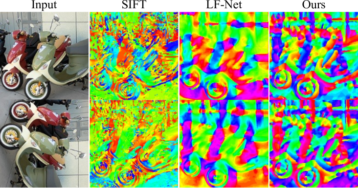
Figure 6: Visualization of the color-coded orientation maps. Upper is the source image, and the bottom is the target image. For the better view, we apply $T^{-1}_{g}$ to the target image as a spatial alignment. We map the orientation range from $[0,359)$ to $[0,255)$ to visualize the orientations by hue of HSV color representation.

5 Conclusion

This paper presents a self-supervised oriented keypoint detection method using rotation-equivariant CNNs. The rotation-equivariant representation with pooling in separate dimensions generates robust features for oriented keypoint detection. The proposed dense orientation alignment loss trains the histograms consistently changing to rotation. Extensive experiments show the effectiveness of the proposed oriented keypoints compared to the existing methods in standard image matching benchmarks. In the future, this study can be extended to the general transformation groups, e.g., affine/non-rigid, or to learning the rotation-equivariant descriptors and joint equivariant learning of the detection and description. We leave this for the future.

Acknowledgement. This work was supported by Samsung Research Funding & Incubation Center of Samsung Electronics under Project Number SRFC-TF2103-02.

Self-Supervised Equivariant Learning for Oriented Keypoint Detection
- Suppelementary material -

In this supplementary material, we explain the reason for the periodic results under synthetic rotations, the effect of the number of keypoints in IMC2021 [21], and the details of the outlier filtering algorithm in section 6. We show additional results on the Extreme Rotation dataset [26], the ablation studies, and the separated results of the HPatches viewpoint/illumination in section 7. We compare the qualitative results of the predicted matches and orientation estimation in section 8.

6 Additional analysis

In section 6.1, we explain the performance variation cycles in Figs.4-5 of the main paper. In section 6.2, we explain why the performance of IMC2021 [21] largely drops from 2,000 points to 8,000 points. In section 6.3, we explain the detailed description of the outlier filtering algorithm.

6.1 Performance variation cycles in Figs.4-5

The periodic patterns in Figs.4-5 of the main paper are caused by input variations due to the grid structure of pixels and the square shape of convolution filters. (1) Since an image is a grid structure of pixels, a rotation of the image induces an interpolation artifact for the corresponding position, being minimal for a multiple of 90°and maximal in between. Fig. 7 plots the average errors from the original pixel values, which clearly show the same cycle. (2) Since convolution filters take a square grid of pixels as input, a rotation of the image makes the filters take a different set of pixels, being the same set again for a multiple of 90°. Therefore, compared to the reference image, the rotated input to the model varies most at 45°, 135°, 225°, 315°rotations, which induces the degrading cycle. The similar pattern can also be found in Fig.7 of ORB [51].

6.2 The effect of the number of keypoints in IMC2021 [21]

Fig.13 and Sec.5.4 in [21] show that the pose estimation accuracy increases until the number of keypoints reaches 8,000 and converges, so [21] adopt the 2,048 and 8,000 numbers of keypoints as standard evaluation protocols. A scene of IMC2021 consists of the exhaustive pairs of 100 images, and the accuracy increases at 8,000 keypoints than 2,048 keypoints as a keypoint in one image is likely to exist in the other images.

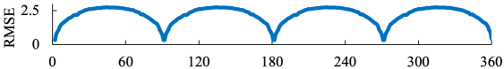
Figure 7: RMSE of the corresponding pixel values in rotating image.

6.3 Detailed descriptions of the outlier filtering

To show the effectiveness of the estimated orientations in Table 3 of the main paper, we use an outlier filtering algorithm. We filter the outlier matches through the global consensus of the orientation values assigned in keypoints of the tentative matches. We compute the orientation difference of two keypoints for each tentative match and then select the most frequent difference from all those tentative matches. This most frequent orientation difference is used to define outlier matches by measuring how large each tentative match deviates from it. Let $\mathbf{m}\in\mathbb{N}^{K\times 2}$ is a set of the tentative matches about the pair of keypoint indices, which is obtained using the mutual nearest neighbour matcher. The inlierness $p$ is defined for a tentative match of two keypoints with orientations $o^{\mathrm{a}}$ and $o^{\mathrm{b}}$:

$${p}(o^{\mathrm{a}},o^{\mathrm{b}},t)=\begin{cases}1,&\text{if }|\text{{mode}}(\vec{d})-d|\leq t,\\ 0,&\text{otherwise,}\end{cases}$$ (16)

$$\text{and }d=(o^{\mathrm{b}}-o^{\mathrm{a}}+360)\bmod 360,$$

where $\vec{d}\in\mathbb{R}^{K}$ is a vector of the orientation differences, mode function returns the most frequent value on the input vector, $t$ is a threshold to accept how far from the frequent orientation difference, and $K$ is the number of tentative matches. We use the outlier threshold $t=30\degree$ for Table 3 in the main paper. Note that $o^{\mathrm{a}}$ and $o^{\mathrm{b}}$ denote two orientation values of a tentative match. We obtain the orientation vector $\vec{o}\in\mathbb{R}^{K}$ of our keypoints as follows:

$$\vec{o}^{\mathrm{\,a}}=\operatorname*{arg\,max}_{g}\delta(\mathbf{O}^{\mathrm{a}};\mathbf{m}_{:,0})_{g},\vec{o}^{\mathrm{\,b}}=\operatorname*{arg\,max}_{g}\delta(\mathbf{O}^{\mathrm{b}};\mathbf{m}_{:,1})_{g},$$ (17)

where $\mathbf{O}\in\mathbb{R}^{|G|\times H\times W}$ is the rotation-equivariant orientation tensor, $\delta:\mathbb{R}^{|G|\times H\times W}\rightarrow\mathbb{N}^{|G|\times K}$ selects the orientation values from the keypoint coordinates using the keypoint indices in tentative matches $\mathbf{m}_{:,i}$, and $g\in G$.

7 Additional results

In section 7.1, we demonstrate the results of keypoint matching on the Extreme Rotation (ER) benchmark [26]. In section 7.2, we show the results of ablation studies. In section 7.3, we show the separated results of the HPatches viewpoint/illumination.

7.1 Evaluation on the ER dataset [26]

Table 5 shows the Percentage of Correctly Matched Keypoints (PCK) in the ER dataset proposed in [26]. The ER dataset contains image pairs with large rotations produced by artificially transforming the images of HPatches [2] and SUN3D [70]. We only use our keypoints without outlier filtering by the orientations in this experiment. Our rotation-invariant keypoint detector improves PCKs by finding the more reliable keypoints within the extreme rotation setting than SuperPoint [14]. In addition, the integration with ours and GIFT [26] achieves the best PCKs compared to the previous best, SuperPoint [14] with GIFT [26], in the ER dataset.

Det.	Des.		PCK@5	PCK@2	PCK@1
SuperPoint [14]	SuperPoint [14]		0.255	0.194	0.112
SuperPoint [14]	GIFT [26]		0.435	0.328	0.186
ours	GIFT [26]		0.476	0.353	0.212

Table 5: PCK on the Extreme Rotation dataset [26]. The numbers next to the PCK represent the pixel threshold to measure the correctness of the correspondence.

7.2 Ablation studies

Loss.	rep.	w/o out. filter.				out. filter.
		MMA		match.		MMA		match.
		@3px	@5px			@3px	@5px
$\mathcal{L}^{\textrm{ori}}$+$\mathcal{L}^{\textrm{kpts}}$	57.6	73.1	79.6	505.8		76.7	82.3	440.1
$\mathcal{L}^{\textrm{ori}}$	30.0	44.4	56.6	403.3		49.6	61.9	291.6
$\mathcal{L}^{\textrm{kpts}}$	50.8	69.8	76.8	358.7		75.2	81.2	226.7

Table 6: Ablation experiment about the dense orientation alignment loss $\mathcal{L}^{\textrm{ori}}$ and the window-based keypoint detection loss $\mathcal{L}^{\textrm{kpts}}$ in HPatches [2]. We use 1,000 keypoints and the HardNet descriptor [37]. ‘out. filter.’ denotes the results with outlier filtering, and ‘match’ denotes the number of predicted matches.

Ablations of the loss functions. Table 6 shows the results without each loss function. Without $\mathcal{L}^{\textrm{kpts}}$ in the second row, the repeatability score is decreased because the model cannot obtain the keypoint at a reliable location, so the performances of matching are also decreased. Although without $\mathcal{L}^{\textrm{ori}}$ in the third row, outlier filtering is working because the rotation-equivariant representation $\mathbf{O}$ groups the rotation information of local patterns by the rotation-equivariant networks. However, using both loss functions as in the first row yields higher MMA with more matches, which shows both loss function contributes to generating reliable oriented keypoints in an image.

Different pooling operators in networks. Table 7 shows the results with different pooling operators to verify the design choice of our networks. We use max pooling, average pooling, and bilinear pooling [26] for the keypoint detection branch when collapsing the group, and $1\times 1$ convolution, average pooling, and max pooling for the orientation estimation branch when collapsing the channel. We experiment with all possible exhaustive pairs of these combinations. As a result, the first row proposed in the main paper is best to use max pooling for keypoint detection and $1\times 1$ convolution for orientation estimation. Collapsing the channel with $1\times 1$ convolution in orientation estimation operates as a weighted sum with the learned kernel, giving richer information than max pooling and average pooling. Max pooling on the orientation branch yields compatible MMAs, but filters the excessive number of the predicted matches. We guess the poor performance of bilinear pooling is overfitting due to the excessive number of model parameters, although the loss converges during training, and the repeatability score of the validation set increases. Note that the bilinear pooling [26] takes a very long time because our keypoint map should compute all regions while GIFT generates only features of the extracted keypoints. Hence, the bilinear pooling is not appropriate to collapse the group of our method.

K	O	rep.	w/o out. filter.				out. filter.
			MMA		match.		MMA		match.
			@3px	@5px			@3px	@5px
Max	1x1Conv	57.6	73.1	79.6	505.8		76.7	82.3	440.1
Max	Avg	54.6	70.6	77.4	483.1		76.2	81.5	397.8
Max	Max	56.0	71.8	78.7	500.3		76.9	82.7	352.1
Avg	1x1Monv	55.7	72.3	78.6	480.6		75.9	81.7	339.6
Avg	Avg	51.0	67.2	75.5	459.5		70.0	78.2	315.4
Avg	Max	51.8	66.8	76.6	495.2		72.3	80.5	292.2
Bilinear	1x1Conv	27.6	42.2	51.2	374.7		50.3	57.8	243.5
Bilinear	Avg	26.0	39.7	48.6	370.1		48.3	55.7	182.3
Bilinear	Max	29.6	43.4	52.6	381.4		53.1	60.5	178.3

Table 7: Results using different pooling operators. Column $\mathbf{K}$ denotes the operators of the keypoint detection branch, and column $\mathbf{O}$ denotes the operators of the orientation estimation branch. We use the same configuration of Table 6.

7.3 Separate results on HPatches

Tab. 8 shows the results of viewpoint/illumination on HPatches. Our rotation-equivariant detector with the group-invariant descriptor, GIFT [26], achieves the highest mean matching accuracy (MMA) overall on both variations. Although ORB [51] shows a higher repeatability under viewpoint changes, the results with our keypoint detector consistently show the better MMAs compared to ORB [51]. The repeatability score of our model is either the best or the second-best for each variation.

Detector	Descriptor	Illumination				Viewpoint
		Rep.	MMA		pred. match.	Rep.	MMA		pred. match.
			@3px	@5px			@3px	@5px
SIFT [27]	SIFT [27]	42.3	48.0	51.0	405.4	41.8	51.0	53.9	406.5
ORB [51]	ORB [51]	54.6	48.1	52.0	378.2	60.0	45.1	48.1	346.3
D2-Net [15]	D2-Net [15]	26.9	47.7	61.8	411	12.9	23.2	35.8	333.9
LF-Net [41]	LF-Net [41]	48.9	56.1	61.3	337.8	38.8	48.1	52.6	322.9
R2D2 [45]	R2D2 [45]	48.5	70.0	80.6	399.3	42.6	59.3	69.2	320.0
SuperPoint [14]	SuperPoint [14]	51.7	68.6	76.2	469.9	42.4	58.5	63.9	467.6
SuperPoint [14]	GIFT [26]	51.7	69.5	77.5	484.2	42.4	68.2	74.6	508.3
Key.Net [3]	HardNet [37]	54.1	70.8	78.3	497.4	57.7	74.1	80.4	452.2
Key.Net [3]	SOSNet [63]	54.1	70.8	78.3	487.9	57.7	74.5	80.9	442.2
Key.Net [3]	HyNet [62]	54.1	69.8	77.3	499.9	57.7	74.1	80.5	451.5
ours	HardNet [37]	57.1	74.0	81.1	556.2	58.1	72.2	78.1	457.1
ours	SOSNet [63]	57.1	74.5	81.6	550.9	58.1	72.4	78.4	449.8
ours	HyNet [62]	57.1	73.5	80.6	555.6	58.1	72.3	78.4	452.8
ours	GIFT [26]	57.1	75.4	81.1	443.6	58.1	75.4	81.1	388.6

Table 8: Separated results on HPatches illumination/viewpoint variations. We evaluate the Key.Net [3] results using the re-trained model with the code provided by the authors. Results in bold indicate the best result, and underlined results indicate the second best results.

8 Qualitative results

Figure 8 qualitatively compares the orientation maps of SIFT [27], LF-Net [41], and ours. We use the synthetic images in Section 4.2 of the main paper. For obtaining the SIFT orientation, we partition an entire image into patches and estimate the dominant orientation of each patch except the boundary regions. Each result consists of three rows. The first rows show the source image and the estimated source orientation maps, and the second rows show the target image and the estimated target orientation maps spatially aligned to the source image with GT homography. In the third rows, we first compute the difference of orientation maps, and then compute the correctness by thresholding the error 15$\degree$ using the ground-truth angle. Our correctness maps consistently keep more pixels as correct, implying that our model produce a more accurate relative orientation of each pixel than SIFT [27] and LF-Net [41].

Figure 9 and 10 show the qualitative results for the HPatches illumination and viewpoint, respectively. We use HardNet descriptor [37] for Key.Net [3] and ours and use their own descriptor for SIFT [27] and LF-Net [41]. We use mutual nearest matcher for all cases. Our model consistently finds the larger number of correct matches (green) and the smaller number of incorrect matches (red) compared to the baselines in the viewpoint and illumination examples.

Figure 11 visualizes the predicted matches on the validation set of Phototourism in IMC2021 [21]. We draw the inliers produced by DEGENSAC [9]. We color the correct matches from green (0 pixel off) to yellow (5 pixels off), and the incorrect matches in red (more than 5 pixels off). Matches with occluding keypoints by changing the camera pose are drawn in blue. In this unconstrained urban scene, our model generates a larger number of correct matches with a smaller number of false positives than the previous keypoint detectors, SIFT+AN [27, 38] and Key.Net [3], in the same image matching pipeline.

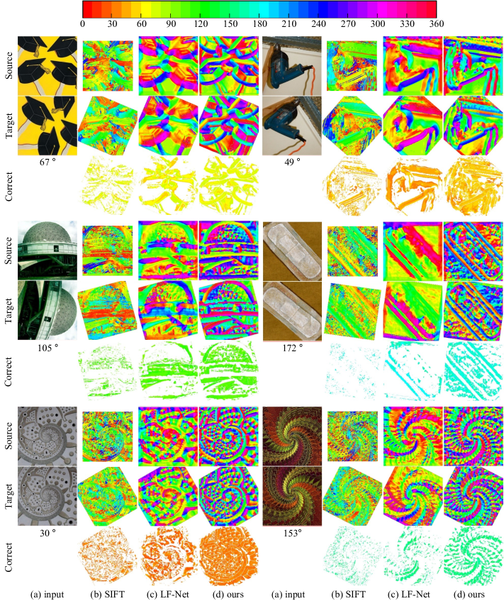
Figure 8: Visualization of the color-coded orientation maps under synthetic rotations with Gaussian noise. We spatially align the orientation map of the target image to the source image using a ground-truth homography for a better view. We create a correctness map between the source orientation map and the aligned orientation map by computing a 15$\degree$ threshold in the third row. The numbers below the target images indicate the ground-truth angles between the source and target images. We use the HSV color representation to visualize the color map of the orientations. The color bar located at the top denotes the corresponding color of orientation degree. Two examples with complicated patterns at the bottom show that our orientation estimator derives more accurate orientations than the existing orientation estimators [27, 41].

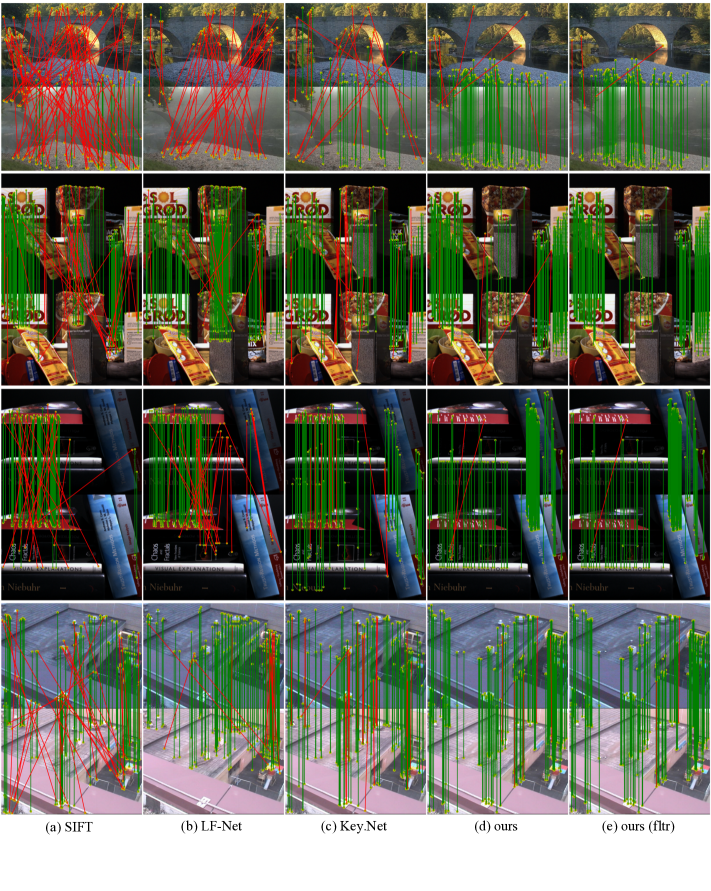
Figure 9: Visualization of the predicted matches in HPatches illumination variations [21]. We detect 300 keypoints for each image and match them by mutual nearest neighbors. The green and red lines indicate correct and incorrect matches, respectively, by a three-pixel threshold. Our rotation-invariant keypoints in column (d) derives smaller number of false-positive matches than columns (a), (b), and (c). Column (e) using the outlier filtering shows that the characteristic orientations effectively filter a set of the correct matches in illumination variations.

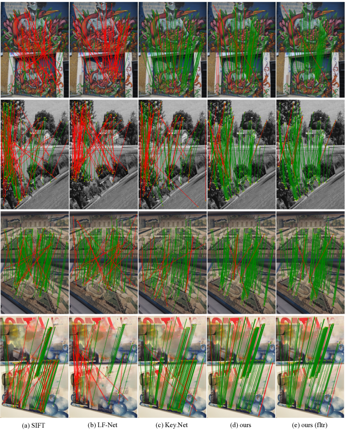
Figure 10: Visualization of the predicted matches in HPatches viewpoint variations [21]. We draw the correct matches (green) and the incorrect matches (red) by a three-pixel threshold. Our oriented keypoint detector with HardNet [37] (column (d), (e)) produce a larger number of matches with a smaller number of false positives in extreme rotation case (row 2) and 3D viewpoint changes (row 1, 3, 4) compared to the columns (a) SIFT [27], (b) LF-Net [41] and (c) Key.Net+HardNet [3, 37].

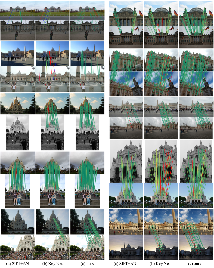
Figure 11: Visualization of the predicted matches in IMC2021 [21], with HardNet descriptor [37], DEGENSAC [9] with AdaLAM [7]. Matches above the 5-pixel error threshold are displayed in red, and matches below are color-coded according to errors between 0 (green) to 5 pixels (yellow). Matches without a depth estimate are displayed in blue. We use 1,024 keypoints to compare with SIFT+AN [27, 38], Key.Net [3], and ours.

References

- [1] Sameer Agarwal, Yasutaka Furukawa, Noah Snavely, Ian Simon, Brian Curless, Steven M Seitz, and Richard Szeliski. Building rome in a day. Communications of the ACM, 54(10):105–112, 2011.
- [2] Vassileios Balntas, Karel Lenc, Andrea Vedaldi, and Krystian Mikolajczyk. Hpatches: A benchmark and evaluation of handcrafted and learned local descriptors. In Proceedings of the IEEE Conference on Computer Vision and Pattern Recognition, pages 5173–5182, 2017.
- [3] Axel Barroso-Laguna, Edgar Riba, Daniel Ponsa, and Krystian Mikolajczyk. Key. net: Keypoint detection by handcrafted and learned cnn filters. In Proceedings of the IEEE/CVF International Conference on Computer Vision, pages 5836–5844, 2019.
- [4] Herbert Bay, Tinne Tuytelaars, and Luc Van Gool. Surf: Speeded up robust features. In European conference on computer vision, pages 404–417. Springer, 2006.
- [5] Paul R Beaudet. Rotationally invariant image operators. In Proc. 4th Int. Joint Conf. Pattern Recog, Tokyo, Japan, 1978, 1978.
- [6] Eric Brachmann and Carsten Rother. Neural-guided ransac: Learning where to sample model hypotheses. In Proceedings of the IEEE/CVF International Conference on Computer Vision, pages 4322–4331, 2019.
- [7] Luca Cavalli, Viktor Larsson, Martin Ralf Oswald, Torsten Sattler, and Marc Pollefeys. Handcrafted outlier detection revisited. In European Conference on Computer Vision, pages 770–787. Springer, 2020.
- [8] Christopher B Choy, JunYoung Gwak, Silvio Savarese, and Manmohan Chandraker. Universal correspondence network. In NeurIPS, pages 2414–2422, 2016.
- [9] Ondrej Chum, Tomas Werner, and Jiri Matas. Two-view geometry estimation unaffected by a dominant plane. In 2005 IEEE Computer Society Conference on Computer Vision and Pattern Recognition (CVPR’05), volume 1, pages 772–779. IEEE, 2005.
- [10] Taco Cohen and Max Welling. Group equivariant convolutional networks. In International conference on machine learning, pages 2990–2999. PMLR, 2016.
- [11] Taco S Cohen, Mario Geiger, and Maurice Weiler. A general theory of equivariant cnns on homogeneous spaces. In Proceedings of the 33rd International Conference on Neural Information Processing Systems, pages 9145–9156, 2019.
- [12] Taco S Cohen and Max Welling. Steerable cnns. arXiv preprint arXiv:1612.08498, 2016.
- [13] Daniel DeTone, Tomasz Malisiewicz, and Andrew Rabinovich. Toward geometric deep slam. arXiv preprint arXiv:1707.07410, 2017.
- [14] Daniel DeTone, Tomasz Malisiewicz, and Andrew Rabinovich. Superpoint: Self-supervised interest point detection and description. In CVPR Deep Learning for Visual SLAM Workshop, 2018.
- [15] Mihai Dusmanu, Ignacio Rocco, Tomas Pajdla, Marc Pollefeys, Josef Sivic, Akihiko Torii, and Torsten Sattler. D2-net: A trainable cnn for joint description and detection of local features. In Proceedings of the ieee/cvf conference on computer vision and pattern recognition, pages 8092–8101, 2019.
- [16] Patrick Ebel, Anastasiia Mishchuk, Kwang Moo Yi, Pascal Fua, and Eduard Trulls. Beyond cartesian representations for local descriptors. In Proceedings of the IEEE/CVF International Conference on Computer Vision, pages 253–262, 2019.
- [17] Jiaming Han, Jian Ding, Nan Xue, and Gui-Song Xia. Redet: A rotation-equivariant detector for aerial object detection. In Proceedings of the IEEE/CVF Conference on Computer Vision and Pattern Recognition, pages 2786–2795, 2021.
- [18] Chris Harris, Mike Stephens, et al. A combined corner and edge detector. In Alvey vision conference, number 50, pages 10–5244. Citeseer, 1988.
- [19] Jared Heinly, Johannes L. Schönberger, Enrique Dunn, and Jan-Michael Frahm. Reconstructing the world* in six days. In 2015 IEEE Conference on Computer Vision and Pattern Recognition (CVPR), pages 3287–3295, 2015.
- [20] Max Jaderberg, Karen Simonyan, Andrew Zisserman, et al. Spatial transformer networks. Advances in neural information processing systems, 28:2017–2025, 2015.
- [21] Yuhe Jin, Dmytro Mishkin, Anastasiia Mishchuk, Jiri Matas, Pascal Fua, Kwang Moo Yi, and Eduard Trulls. Image matching across wide baselines: From paper to practice. International Journal of Computer Vision, 129(2):517–547, 2021.
- [22] Nick Kanopoulos, Nagesh Vasanthavada, and Robert L Baker. Design of an image edge detection filter using the sobel operator. IEEE Journal of solid-state circuits, 23(2):358–367, 1988.
- [23] Jongmin Lee, Yoonwoo Jeong, and Minsu Cho. Self-supervised learning of image scale and orientation. In 31st British Machine Vision Conference (BMVC) 2021, Virtual Event, UK. BMVA Press, 2021.
- [24] Jongmin Lee, Yoonwoo Jeong, Seungwook Kim, Juhong Min, and Minsu Cho. Learning to distill convolutional features into compact local descriptors. In Proceedings of the IEEE/CVF Winter Conference on Applications of Computer Vision, pages 898–908, 2021.
- [25] Karel Lenc and Andrea Vedaldi. Learning covariant feature detectors. In European conference on computer vision, pages 100–117. Springer, 2016.
- [26] Yuan Liu, Zehong Shen, Zhixuan Lin, Sida Peng, Hujun Bao, and Xiaowei Zhou. Gift: Learning transformation-invariant dense visual descriptors via group cnns. Advances in Neural Information Processing Systems, 32:6992–7003, 2019.
- [27] David G Lowe. Distinctive image features from scale-invariant keypoints. International journal of computer vision, 60(2):91–110, 2004.
- [28] Simon Lynen, Bernhard Zeisl, Dror Aiger, Michael Bosse, Joel Hesch, Marc Pollefeys, Roland Siegwart, and Torsten Sattler. Large-scale, real-time visual–inertial localization revisited. The International Journal of Robotics Research, 39(9):1061–1084, 2020.
- [29] Diego Marcos, Michele Volpi, Nikos Komodakis, and Devis Tuia. Rotation equivariant vector field networks. In Proceedings of the IEEE International Conference on Computer Vision, pages 5048–5057, 2017.
- [30] Roland Memisevic. On multi-view feature learning. In ICML, 2012.
- [31] Roland Memisevic and Geoffrey E Hinton. Learning to represent spatial transformations with factored higher-order boltzmann machines. Neural computation, 22(6):1473–1492, 2010.
- [32] Krystian Mikolajczyk and Cordelia Schmid. Scale & affine invariant interest point detectors. International journal of computer vision, 60(1):63–86, 2004.
- [33] Krystian Mikolajczyk and Cordelia Schmid. A performance evaluation of local descriptors. IEEE transactions on pattern analysis and machine intelligence, 27(10):1615–1630, 2005.
- [34] Krystian Mikolajczyk, Tinne Tuytelaars, Cordelia Schmid, Andrew Zisserman, Jiri Matas, Frederik Schaffalitzky, Timor Kadir, and Luc Van Gool. A comparison of affine region detectors. International journal of computer vision, 65(1):43–72, 2005.
- [35] Juhong Min, Jongmin Lee, Jean Ponce, and Minsu Cho. Hyperpixel flow: Semantic correspondence with multi-layer neural features. In ICCV, 2019.
- [36] Juhong Min, Jongmin Lee, Jean Ponce, and Minsu Cho. Learning to compose hypercolumns for visual correspondence. In Computer Vision–ECCV 2020: 16th European Conference, Glasgow, UK, August 23–28, 2020, Proceedings, Part XV 16, pages 346–363. Springer, 2020.
- [37] Anastasiia Mishchuk, Dmytro Mishkin, Filip Radenovic, and Jiri Matas. Working hard to know your neighbor’s margins: Local descriptor learning loss. In Advances in Neural Information Processing Systems, pages 4826–4837, 2017.
- [38] Dmytro Mishkin, Filip Radenovic, and Jiri Matas. Repeatability is not enough: Learning affine regions via discriminability. In Proceedings of the European Conference on Computer Vision (ECCV), pages 284–300, 2018.
- [39] Raul Mur-Artal, Jose Maria Martinez Montiel, and Juan D Tardos. Orb-slam: a versatile and accurate monocular slam system. IEEE transactions on robotics, 31(5):1147–1163, 2015.
- [40] Hyeonwoo Noh, Andre Araujo, Jack Sim, Tobias Weyand, and Bohyung Han. Large-scale image retrieval with attentive deep local features. In Proceedings of the IEEE international conference on computer vision, pages 3456–3465, 2017.
- [41] Yuki Ono, Eduard Trulls, Pascal Fua, and Kwang Moo Yi. Lf-net: learning local features from images. In Advances in neural information processing systems, pages 6234–6244, 2018.
- [42] Adam Paszke, Sam Gross, Francisco Massa, Adam Lerer, James Bradbury, Gregory Chanan, Trevor Killeen, Zeming Lin, Natalia Gimelshein, Luca Antiga, et al. Pytorch: An imperative style, high-performance deep learning library. Advances in neural information processing systems, 32:8026–8037, 2019.
- [43] Rémi Pautrat, Viktor Larsson, Martin R Oswald, and Marc Pollefeys. Online invariance selection for local feature descriptors. In European Conference on Computer Vision, pages 707–724. Springer, 2020.
- [44] Nicolas Pielawski, Elisabeth Wetzer, Johan Öfverstedt, Jiahao Lu, Carolina Wählby, Joakim Lindblad, and Nataša Sladoje. CoMIR: Contrastive multimodal image representation for registration. In H. Larochelle, M. Ranzato, R. Hadsell, M. F. Balcan, and H. Lin, editors, Advances in Neural Information Processing Systems, volume 33, pages 18433–18444. Curran Associates, Inc., 2020.
- [45] Jerome Revaud, Cesar De Souza, Martin Humenberger, and Philippe Weinzaepfel. R2d2: Reliable and repeatable detector and descriptor. Advances in neural information processing systems, 32:12405–12415, 2019.
- [46] Edgar Riba, Dmytro Mishkin, Daniel Ponsa, Ethan Rublee, and Gary Bradski. Kornia: an open source differentiable computer vision library for pytorch. In Proceedings of the IEEE/CVF Winter Conference on Applications of Computer Vision, pages 3674–3683, 2020.
- [47] Ignacio Rocco, Relja Arandjelović, and Josef Sivic. Efficient neighbourhood consensus networks via submanifold sparse convolutions. In European Conference on Computer Vision, pages 605–621. Springer, 2020.
- [48] Ignacio Rocco, Mircea Cimpoi, Relja Arandjelović, Akihiko Torii, Tomas Pajdla, and Josef Sivic. Neighbourhood consensus networks. In NeurIPS, pages 1656–1667, 2018.
- [49] Paul L Rosin. Measuring corner properties. Computer Vision and Image Understanding, 73(2):291–307, 1999.
- [50] Edward Rosten and Tom Drummond. Machine learning for high-speed corner detection. In European conference on computer vision, pages 430–443. Springer, 2006.
- [51] Ethan Rublee, Vincent Rabaud, Kurt Konolige, and Gary Bradski. Orb: An efficient alternative to sift or surf. In 2011 International conference on computer vision, pages 2564–2571. Ieee, 2011.
- [52] Olga Russakovsky, Jia Deng, Hao Su, Jonathan Krause, Sanjeev Satheesh, Sean Ma, Zhiheng Huang, Andrej Karpathy, Aditya Khosla, Michael Bernstein, Alexander C. Berg, and Li Fei-Fei. ImageNet Large Scale Visual Recognition Challenge. International Journal of Computer Vision (IJCV), 115(3):211–252, 2015.
- [53] Paul-Edouard Sarlin, Daniel DeTone, Tomasz Malisiewicz, and Andrew Rabinovich. Superglue: Learning feature matching with graph neural networks. In Proceedings of the IEEE/CVF conference on computer vision and pattern recognition, pages 4938–4947, 2020.
- [54] Torsten Sattler, Bastian Leibe, and Leif Kobbelt. Improving image-based localization by active correspondence search. In European conference on computer vision, pages 752–765. Springer, 2012.
- [55] Torsten Sattler, Will Maddern, Carl Toft, Akihiko Torii, Lars Hammarstrand, Erik Stenborg, Daniel Safari, Masatoshi Okutomi, Marc Pollefeys, Josef Sivic, et al. Benchmarking 6dof outdoor visual localization in changing conditions. In Proceedings of the IEEE Conference on Computer Vision and Pattern Recognition, pages 8601–8610, 2018.
- [56] Nikolay Savinov, Akihito Seki, Lubor Ladicky, Torsten Sattler, and Marc Pollefeys. Quad-networks: unsupervised learning to rank for interest point detection. In Proceedings of the IEEE conference on computer vision and pattern recognition, pages 1822–1830, 2017.
- [57] Johannes L Schonberger and Jan-Michael Frahm. Structure-from-motion revisited. In Proceedings of the IEEE conference on computer vision and pattern recognition, pages 4104–4113, 2016.
- [58] Xuelun Shen, Cheng Wang, Xin Li, Zenglei Yu, Jonathan Li, Chenglu Wen, Ming Cheng, and Zijian He. Rf-net: An end-to-end image matching network based on receptive field. In Proceedings of the IEEE Conference on Computer Vision and Pattern Recognition, pages 8132–8140, 2019.
- [59] Kihyuk Sohn and Honglak Lee. Learning invariant representations with local transformations. In ICML, 2012.
- [60] Ivan Sosnovik, Michał Szmaja, and Arnold Smeulders. Scale-equivariant steerable networks. In International Conference on Learning Representations, 2020.
- [61] Suwichaya Suwanwimolkul, Satoshi Komorita, and Kazuyuki Tasaka. Learning of low-level feature keypoints for accurate and robust detection. In Proceedings of the IEEE/CVF Winter Conference on Applications of Computer Vision, pages 2262–2271, 2021.
- [62] Yurun Tian, Axel Barroso Laguna, Tony Ng, Vassileios Balntas, and Krystian Mikolajczyk. Hynet: Learning local descriptor with hybrid similarity measure and triplet loss. Advances in Neural Information Processing Systems, 33, 2020.
- [63] Yurun Tian, Xin Yu, Bin Fan, Fuchao Wu, Huub Heijnen, and Vassileios Balntas. Sosnet: Second order similarity regularization for local descriptor learning. In Proceedings of the IEEE/CVF Conference on Computer Vision and Pattern Recognition, pages 11016–11025, 2019.
- [64] Prune Truong, Martin Danelljan, and Radu Timofte. Glu-net: Global-local universal network for dense flow and correspondences. In Proceedings of the IEEE/CVF conference on computer vision and pattern recognition, pages 6258–6268, 2020.
- [65] Michal Jan Tyszkiewicz, Pascal Fua, and Eduard Trulls. Disk: learning local features with policy gradient. Advances in Neural Information Processing Systems, 33, 2020.
- [66] Yannick Verdie, Kwang Yi, Pascal Fua, and Vincent Lepetit. Tilde: A temporally invariant learned detector. In Proceedings of the IEEE conference on computer vision and pattern recognition, pages 5279–5288, 2015.
- [67] Maurice Weiler and Gabriele Cesa. General e (2)-equivariant steerable cnns. Advances in Neural Information Processing Systems, 32:14334–14345, 2019.
- [68] Maurice Weiler, Fred A Hamprecht, and Martin Storath. Learning steerable filters for rotation equivariant cnns. In Proceedings of the IEEE Conference on Computer Vision and Pattern Recognition, pages 849–858, 2018.
- [69] Daniel E Worrall, Stephan J Garbin, Daniyar Turmukhambetov, and Gabriel J Brostow. Harmonic networks: Deep translation and rotation equivariance. In Proceedings of the IEEE Conference on Computer Vision and Pattern Recognition, pages 5028–5037, 2017.
- [70] Jianxiong Xiao, Andrew Owens, and Antonio Torralba. Sun3d: A database of big spaces reconstructed using sfm and object labels. In Proceedings of the IEEE international conference on computer vision, pages 1625–1632, 2013.
- [71] Kwang Moo Yi, Eduard Trulls, Vincent Lepetit, and Pascal Fua. Lift: Learned invariant feature transform. In European conference on computer vision, pages 467–483. Springer, 2016.
- [72] Kwang Moo Yi, Eduard Trulls, Yuki Ono, Vincent Lepetit, Mathieu Salzmann, and Pascal Fua. Learning to find good correspondences. In Proceedings of the IEEE conference on computer vision and pattern recognition, pages 2666–2674, 2018.
- [73] Kwang Moo Yi, Yannick Verdie, Pascal Fua, and Vincent Lepetit. Learning to assign orientations to feature points. In Proceedings of the IEEE conference on computer vision and pattern recognition, pages 107–116, 2016.
- [74] Jiahui Zhang, Dawei Sun, Zixin Luo, Anbang Yao, Lei Zhou, Tianwei Shen, Yurong Chen, Long Quan, and Hongen Liao. Learning two-view correspondences and geometry using order-aware network. In Proceedings of the IEEE/CVF International Conference on Computer Vision, pages 5845–5854, 2019.
- [75] Xu Zhang, Felix X Yu, Svebor Karaman, and Shih-Fu Chang. Learning discriminative and transformation covariant local feature detectors. In Proceedings of the IEEE conference on computer vision and pattern recognition, pages 6818–6826, 2017.
- [76] Yanzhao Zhou, Qixiang Ye, Qiang Qiu, and Jianbin Jiao. Oriented response networks. In Proceedings of the IEEE Conference on Computer Vision and Pattern Recognition, pages 519–528, 2017.
- [77] Siyu Zhu, Runze Zhang, Lei Zhou, Tianwei Shen, Tian Fang, Ping Tan, and Long Quan. Very large-scale global sfm by distributed motion averaging. In Proceedings of the IEEE conference on computer vision and pattern recognition, pages 4568–4577, 2018.