Extremely Correlated Fermi Liquid theory for $U=\infty$, $d=\infty$ Hubbard model to ${\cal O}(\lambda^{3})$

Abstract

We present the ${\cal O}(\lambda^{3})$ results from the $\lambda$ expansion in the extremely correlated Fermi liquid theory applied to the infinite-dimensional  $t$-$J$  model (with $J=0$), and compare the results with the earlier ${\cal O}(\lambda^{2})$ results as well as the results from the dynamical mean field theory. We focus attention on the $T$ dependence of the resistivity $\rho(T)$, the Dyson self energy, and the quasiparticle weight $Z$ at various densities. The comparison shows that all the methods display quadratic in T resistivity followed by a quasi-linear in T resistivity characterizing a strange metal, and gives an estimate of the different scales of these variables relative to the exact results.

1 Introduction

The  $t$-$J$  model Eq. (1) provides an important context for understanding strongly correlated systems. It is closely related to the $U\gg t$ Gutzwiller-Hubbard-Kanamori [1] model. It is formally equivalent to the $U=\infty$ model to which we add superexchange interactions Eq. (1). It can be obtained from a canonical transformation on the Hubbard model for large $U$, provided we throw out certain three center terms of ${\cal O}(t^{2}/U)$ [2]. In previous papers [3, 4, 5] we have developed the extremely correlated Fermi liquid (ECFL) theory to overcome the most difficult features of the model, namely the $U=\infty$ limit which eliminates a substantial fraction of states in the Hilbert space corresponding to double occupation of sites. The resulting electrons are termed as Gutzwiller projected electrons, satisfying a non-canonical algebra Eq. (2). As a result the Feynman diagram based perturbation theory fails here, and this motivated the development of the ECFL theory as described elsewhere.

We note that the importance of the physics of strong correlations has motivated considerable activity in the theoretical community. On the analytical side, the dynamical mean field theory (DMFT) [6, 7, 8, 9, 10, 11, 12, 13] has matured into a reliable tool. It uses the numerical renormalization group of Wilson and Krishnamurthy[14, 15] for a generalized Anderson impurity model, and provides exact numerical results for the case of infinite dimension, which is the focus of the current work using ECFL.

The ECFL theory is based on an expansion in a parameter $\lambda$ that is analogous to an expansion of magnetic system models such as the Heisenberg model, for large spin, i.e. an expansion of relevant equations in powers of $\frac{1}{2S}$. The main underlying observation [5, 4, 3] is that the algebra of the Gutzwiller projected electrons is similar to that of the Lie algebra of spin operators, and hence allows the introduction of such a parameter that enables a systematic expansion in powers of $\lambda$. The theory has been developed so far using the ${\cal O}(\lambda^{2})$ expressions for the self energies in the problem, and applied in a variety of situations including $d=0$ i.e. the Anderson impurity model [16], the $d=1$ $t$-$J$  model [17], the $d=\infty,U=\infty$ Hubbard model [18, 19] and closest to experiments, the $d=2$ $t$-$J$  model [20, 21, 22]. At a formal level we have also established a systematic method for extending the expansion to high order terms, but in view of the additional technical difficulties presented by them, the effect of the higher order terms have not yet been tested. This work reports the first results from the third order equations for the ECFL, applied to the case of the $d=\infty$ and $U=\infty$ Hubbard model. The results are compared with results from DMFT as well as with earlier 2nd order equations.

In Section. (2) we summarize the basic aspects of the ECFL theory. We define the  $t$-$J$  model and give an expression for the single electron Greens function of the Gutzwiller projected electrons, and the two self energies involved in the construction. We summarize the various approaches to the $\lambda$ expansion method, and explain the ideas behind the shift invariance of the equations, which are of great importance in the  $t$-$J$  model. We then summarize the second and third order expressions for the self energies and cast these in a form that is convenient for computation.

In Section (3) we discuss the two sum-rules employed to fix the two Lagrange multipliers in the problem. While one of them is the familiar particle number sum-rule, the other arises from the exact equations of motion of the Greens function, as derived in Appendix. (A).

Section. (4) presents the calculated results from the second and third order expansions. We focus attention on the $T$ dependence of the resistivity $\rho(T)$, the Dyson self energy, and the quasiparticle weight $Z$ at various densities. We compare these results between the successive approximations, the exact DMFT results and also the so called Tukey window scheme used earlier by us.

2 Basic Theory

2.1 ECFL theory Formulas for ${\cal G}$

The general formalism underlying the theory of extremely correlated Fermi liquids (ECFL) has been discussed extensively in recent works[4, 5, 26, 25, 24]. Here we record the equations relevant to the present work, and point out the origin of the main equations in earlier works in detail . We start here with the  $t$-$J$  model

$$H=-\sum_{ij\sigma}t_{ij}\widetilde{C}_{i\sigma}^{\dagger}\widetilde{C}_{j\sigma}-{\bm{\mu}}\sum_{i\sigma}\widetilde{C}_{i\sigma}^{\dagger}\widetilde{C}_{i\sigma}+\frac{1}{2}\sum_{ij}J_{ij}\left(\vec{S}_{i}.\vec{S}_{j}-\frac{n_{i}n_{j}}{4}\right),$$ (1)

where $t_{ij}$ are the band hopping parameters whose Fourier transform $\varepsilon_{k}$ is the band energy, $n_{i}=\sum_{i\sigma}\widetilde{C}_{i\sigma}^{\dagger}\widetilde{C}_{i\sigma}$ is the number operator at site $i$, and $\widetilde{C}^{\dagger}_{j\sigma},\widetilde{C}_{i\sigma}$ are Gutzwiller projected fermion operators[4, 5] satisfying non-canonical anticommutators

$$\{\widetilde{C}_{i\sigma_{i}},\widetilde{C}_{j\sigma_{j}}^{\dagger}\}=\delta_{ij}\left(\delta_{\sigma_{i}\sigma_{j}}-\sigma_{i}\sigma_{j}\widetilde{C}_{i\bar{\sigma}_{i}}^{\dagger}\widetilde{C}_{i\bar{\sigma}_{j}}\right),\mbox{and }\{\widetilde{C}_{i\sigma_{i}},\widetilde{C}_{j\sigma_{j}}\}=0.$$ (2)

In ECFL theory, the Green’s function for the  $t$-$J$  model is given as the product of an auxiliary (canonical) Green’s function g and a caparison function $\widetilde{\mu}$:

$${\cal G}(k,i\omega_{m})=\textbf{g}(k,i\omega_{m})\times\widetilde{\mu}(k,i\omega_{m}),$$ (3)

with the fermionic Matsubara frequency $\omega_{m}=k_{B}T(2m+1)\pi$ and $k(=\vec{k})$ is the wave number. These factors of ${\cal G}$ are expressed in terms of self energies $\Psi$ and $\Phi$ as

$$\widetilde{\mu}(k,i\omega_{m}) = 1-\frac{n}{2}+\Psi(k,i\omega_{m}),$$ (4)

$${\bf g}^{-1}(k,i\omega_{m}) = i\omega_{m}+{\bm{\mu}}-(1-\frac{n}{2})\varepsilon_{k}-\Phi(k,i\omega_{m}),$$ (5)

where $n$ is the number of electrons of both spin per site

$$n=\langle n_{i}\rangle=\frac{2}{\beta N_{s}}\sum_{k,m}e^{i\omega_{m}0^{+}}{\cal G}(k,i\omega_{m})$$ (6)

and $N_{s}$ is the number of sites in the lattice, and we set the lattice constant $a_{0}\to 1$. Here $\Phi$ plays the role of a Dyson-type self-energy for the canonical Green’s function $\textbf{g}(k,i\omega_{n})$ and $\Psi$ is a frequency dependent correction to $\widetilde{\mu}(k)$. These equations are valid in any dimension, and have been employed in different works in the special cases of $d=\infty$[26, 25, 18, 19, 27], $d=1$[17] and $d=2$[20, 21, 22].

In this work we specialize to the $d=\infty$ case, which is convenient for the purpose of studying the systematics of the $\lambda$ expansion[4, 5, 24]. Here we set $J=0$ in Eq. (1) and deal with what amounts to the $U=\infty$ Hubbard model. In this limit the self energies simplify[26, 25] to the following $k$ independent expressions

$$\Psi(k,i\omega_{n})=\Psi(i\omega_{n})$$ (7)

$$\Phi(k,i\omega_{n})=\chi(i\omega_{n})+\varepsilon_{k}\Psi(i\omega_{n}).$$ (8)

Here we observe that the entire $\vec{k}$ dependence of $\Phi$ is contained in the band energy $\varepsilon_{k}$. Therefore it follows that we can use $\varepsilon$ as a proxy for the wave vector. We thus combine Eq. (4, 5, 8) to write

$${\bf g}^{-1}=i\omega_{n}+{\bm{\mu}}-\widetilde{\mu}(i\omega_{n})\varepsilon_{k}-\chi(k,i\omega_{n}).$$ (9)

This equation, together with Eq. (4) and Eq. (3) determines the physical Green’s function ${\cal G}$. Combining them we can formally write ${\cal G}$ in the standard Dyson form

$${\cal G}(k,i\omega_{n}) = \frac{1}{{\bf g}^{-1}_{0}(k,i\omega_{n})-\Sigma_{D}(i\omega_{n})}$$ (10)

where ${\bf g}^{-1}_{0}(k,i\omega_{n})=i\omega_{n}+{\bm{\mu}}-\varepsilon_{k}$, and the manifestly $k$ independent Dyson self energy $\Sigma_{D}$ as

$$\Sigma_{D}(i\omega_{n})=i\omega_{n}+{\bm{\mu}}+\frac{\chi(i\omega_{n})-i\omega_{n}-{\bm{\mu}}}{1-\frac{n}{2}+\Psi(i\omega_{n})}.$$ (11)

For later use we record the positive definite electron spectral function $\rho_{{\cal G}}(k,\omega)$ obtained by analytic continuation of ${\cal G}$ in Eq. (10):

$$\rho_{{\cal G}}(k,\omega)=-\frac{1}{\pi}\mathrm{Im}\,{\cal G}(k,i\omega_{n})\bigg{|}_{i\omega_{n}\to\omega+i0^{+}}.$$ (12)

In experimental literature the spectral function $\rho_{{\cal G}}(k,\omega)$ is denoted by $A(k,\omega)$. Following Eq. (12) we define a spectral function obtained from ${\bf g}$ following the same procedure

$$\rho_{{\bf g}}(k,\omega)=-\frac{1}{\pi}\mathrm{Im}\,{\bf g}(k,i\omega_{n})\bigg{|}_{i\omega_{n}\to\omega+i0^{+}}.$$ (13)

Unlike $\rho_{{\cal G}}$, the variable $\rho_{{\bf g}}$ is a mathematical object used in calculations that finally yield the physical spectral function $\rho_{G}$. We perform calculations of the generalized self energies $\chi,\Psi$ in a power series in $\lambda$ with coefficients that depend on ${\bf g}$ (rather than ${\cal G}$), as described below. This expansion determines the Dyson self energy $\Sigma_{D}$ through the rather complicated formula Eq. (11), which is in the form of a ratio of two expressions. This illustrates the advantage of the ECFL formalism, which generates a highly non-trivial $\Sigma_{D}$, through relatively simple self energies $\chi,\Psi$ given below.

2.2 The $\lambda$-expansion:

A basic tool in the ECFL theory is an expansion of the fundamental, and in general intractable functional differential equations, in powers of a parameter $\lambda$ [3, 4, 23]. This parameter is a particular type of counter of the expansion, and is set to unity after isolating its different powers in the expansion of any physical quantity, such as the Greens function, or a self energy. As explained in [4] (see in particular Eqs. (1,2,3,4,5)), the inspiration for the $\lambda$ expansion originally came from an observation in the case of the Hubbard model. Herein the entire set of Feynman diagrams can be obtained by a similar expansion of exact functional differential equations in powers of the interaction constant $U$. The strategy is then to find corresponding functional differential equations for the non-canonical Gutzwiller projected electrons of the  $t$-$J$  model, and to invent a parameter that plays the role of $U$ in the Hubbard, albeit with a limited range. This program can be carried out systematically in three independent ways, as discussed next.

• $\bullet$ Term-by-term iteration, i.e. ${\cal O}(\lambda^{n})$ terms found by taking functional derivative of terms of ${\cal O}(\lambda^{n-1})$ [3, 4, 5], i.e.

  It can be introduced as a parameter in the exact Schwinger-Tomonaga functional differential equations determining the Green’s functions [3, 4], followed by a systematic expansion of these equations[3, 4, 5, 24]. The expansion itself can be done by taking successive functional derivatives of previous terms, as in [3, 4, 5].

• $\bullet$ Generalized diagrams of ${\cal O}(\lambda^{n})$ [24]

  Yet another method of expansion is through a diagrammatic expansion [24], modeled after the Feynman graph representation of terms in the Schwinger-Tomonaga expansion. It brings in a new class of diagrams, outside the category described in Feynman diagrams, thanks to the non-canonical nature of the fermion algebra Eq. (2). The paper [24] gives the systematics of this procedure providing rules extending the Feynman diagram rules. With the help of the new set of rules, one can write down expressions for terms to an arbitrary order $n$ without having to list terms of a lower order $n-1$. This prior order listing is mandatory in the method [A], where we functionally differentiate terms of ${\cal O}(\lambda^{n-1})$ to generate terms of ${\cal O}(\lambda^{n})$.

• $\bullet$ $\lambda$-fermions Eq. (14), and their equations of motion of to ${\cal O}(\lambda^{n})$ [5].

  Finally, and most directly, we can introduce $\lambda$ through a generalization of the anticommutation relations Eq. (2), by writing the anticommutators [5]

  $$\{\widetilde{C}_{i\sigma_{i}},\widetilde{C}_{j\sigma_{j}}^{\dagger}\}=\delta_{ij}\left(\delta_{\sigma_{i}\sigma_{j}}-\,\lambda\,\sigma_{i}\sigma_{j}\widetilde{C}_{i\bar{\sigma}_{i}}^{\dagger}\widetilde{C}_{i\bar{\sigma}_{j}}\right),$$ (14)

  where $\lambda\in[0,1]$. These anticommutators, together with $\{\widetilde{C}_{i\sigma_{i}},\widetilde{C}_{j\sigma_{j}}\}=0$ constitute a Lie algebra that defines $\lambda$-fermions, introduced in (Ref.[5] Sec.5). At $\lambda$=1 we recover the Gutzwiller fermions Eq. (2), while at $\lambda$=0 we recover canonical fermions. The introduction of these $\lambda$-fermions allows us to interpolate continuously between canonical fermions and Gutzwiller projected fermions. The anticommutators are realized in terms of the canonical fermions using the correspondence [5]

  $$\widetilde{C}_{j\sigma_{j}}^{\dagger}\to{C}_{j\sigma_{j}}^{\dagger}(1-\lambda C_{j\bar{\sigma}_{j}}^{\dagger}C_{j\bar{\sigma}_{j}}),\;\widetilde{C}_{j\sigma_{j}}\to{C}_{j\sigma_{j}},\;\mbox{ and }\widetilde{C}_{i\bar{\sigma}_{i}}^{\dagger}\widetilde{C}_{i\bar{\sigma}_{j}}\to{C}_{i\bar{\sigma}_{i}}^{\dagger}{C}_{i\bar{\sigma}_{j}}.$$ (15)

  The equations for the Green’s functions for these $\lambda-$fermions can be similarly expanded systematically in powers of $\lambda$ leading to expressions for the twin self energies and other objects to each order in $\lambda$

  This procedure has a close parallel in the familiar Kubo-Anderson spin-wave expansion encountered in quantum magnets. In the version of that expansion, due to Freeman Dyson [28], the usual angular momentum Lie-algebra with spin-s:

  $$[S_{i}^{\alpha},S_{j}^{\beta}]=i\,\delta_{ij}\,\varepsilon^{\alpha\beta\gamma}\;S_{i}^{\gamma},\mbox{ and }\;\vec{S}_{j}.\vec{S}_{j}=s(s+1),$$ (16)

  is realized using canonical bosons $b_{i},b_{i}^{\dagger}$ their number operator $n_{i}=b_{i}^{\dagger}b_{i}$ with the correspondence

  $$S_{i}^{-}=b_{i},\;S_{i}^{+}=(2s)b_{i}^{\dagger}\left(1-\frac{n_{i}}{2s}\right),\;\mbox{ and }S_{i}^{z}=n_{i}-s,$$ (17)

  together with a projection operator $P_{D}$ that ensures that the number of bosons per site is constrained to the finite number $n_{i}\leq 2s$. Proceeding in this way Dyson and Maleev[28, 29] showed that a formal series in powers of $\frac{1}{2S}$ is possible for physically relevant variables. It is therefore clear that this version of spin wave expansion of quantum-magnets is parallel to the $\lambda$-expansion of Eq. (14) with the mapping $\lambda\leftrightarrow\frac{1}{2S}$. Details and references to applications in quantum magnets using this approach are discussed in [5].

Finally it is worth mentioning that a qualitative understanding of this parameter $\lambda$ can be found in the simple context of a single site model. Here it can be seen explicitly that varying $\lambda$ in the range $\lambda\in[0,1]$ controls the fraction of double occupancy between its uncorrelated value and 0 (see [4] Appendix-A).

2.3 The Shift invariance and the second chemical potential $u_{0}$

At this stage we recall that the  $t$-$J$  model has a simple invariance property

$${\bm{\mu}}\to{\bm{\mu}}-\frac{1}{2}u_{0},\;\;\varepsilon_{k}\to\varepsilon_{k}-\frac{1}{2}u_{0}.$$ (18)

This property expresses the invariance of the band model, when the center of gravity of the band is shifted by an arbitrary constant $\frac{1}{2}u_{0}$. We refer to $u_{0}$ as the second chemical potential of the problem, requiring a second constraint in addition to the number sumrule Eq. (6). It becomes a strong constraint in the ECFL theory, when we insist that Eq. (18) should be preserved to each order in the $\lambda$ expansion. The freedom of choosing $u_{0}$ can be utilized to impose a subsidiary constraint on ${\bf g}$, as discussed below.

For imposing this invariance, we will accordingly shift both ${\bm{\mu}}$ and $\varepsilon_{k}$ in Eq. (5, 8, 9, 11). With this change, and by incorporating the factors of $\lambda$ mentioned above, we record the basic equations Eq. (4, 5, 9) with a factor of $\lambda$ multiplying the relevant terms as well as the constant $u_{0}$ subtracted from ${\bm{\mu}}$ as well as $\varepsilon_{k}$, as derived in [27, 30]

$$\widetilde{\mu}(k,i\omega_{n}) = 1-\lambda\frac{n}{2}+\lambda\Psi(k,i\omega_{n}),$$ (19)

$${\bf g}^{-1}(k) = i\omega_{n}+{\bm{\mu}}-\frac{u_{0}}{2}-(\varepsilon_{k}-\frac{u_{0}}{2})\widetilde{\mu}(i\omega_{n})-\lambda\,\chi(i\omega_{n})$$ (20)

From Eq. (19) it follows that when $\lambda\to 0$, we get $\widetilde{\mu}\to 1$ and hence ${\bf g}$ reduces to the non-interacting Green’s function. The task undertaken in the next section is an expansion of this equation together with Eq. (20) in powers of $\lambda$, giving ${\bf g}^{-1}$ and $\widetilde{\mu}$ to ${\cal O}(\lambda^{3})$. Since $\Psi$ and $\chi$ have a prefactor of $\lambda$, their expansion to (${\cal O}(\lambda)$) ${\cal O}(\lambda^{2})$ generates an expansion to (${\cal O}(\lambda^{2})$) ${\cal O}(\lambda^{3})$ of $\widetilde{\mu}$ and ${\bf g}^{-1}$. The ${\cal O}(\lambda^{2})$ and ${\cal O}(\lambda^{3})$ expressions are taken from [27, 30] and [24].

2.4 The $\lambda$ expansion for the self energies

We expand the two self energies $\Psi,\chi$ (see Eq. (4, 19, 20)) in powers of $\lambda$ as

$$\Psi = \Psi_{[0]}+\lambda\Psi_{[1]}+\lambda^{2}\Psi_{[2]}+\ldots$$ (21)

$$\chi = \chi_{[0]}+\lambda\chi_{[1]}+\lambda^{2}\chi_{[2]}+\ldots$$ (22)

which suffices to determine $\widetilde{\mu}$ and ${\bf g}^{-1}$ to ${\cal O}(\lambda^{3})$. We first record the lowest order terms [24]

$$\Psi_{[0]}=0,$$ (23)

$$\chi_{[0]}=-\sum_{p}{\bf g}(p)e^{i\omega_{p}0^{+}}(\varepsilon_{p}-\frac{u_{0}}{2})=\frac{u_{0}n_{g}}{4}-\sum_{p}{\bf g}(p)\varepsilon_{p}e^{i\omega_{p}0^{+}},$$ (24)

where $\sum_{p}\equiv\frac{k_{B}T}{N_{s}}\sum_{\vec{p}\omega_{p}}$, and $N_{s}$ is the number of lattice sites. We defined $n_{g}$ using

$$n_{g}=2\sum_{p}{\bf g}(p)e^{i\omega_{p}0^{+}}.$$ (25)

For brevity the factor $e^{i\omega_{p}0^{+}}$ is omitted in the following, whenever we sum over a single ${\bf g}$. Here $n_{g}$ is a formal construct and should not be confused with the number density of physical electrons $n$, the latter is given in terms of ${\cal G}$ in Eq. (6). In practice $n_{g}$ turns out to be quite close to $n$ at low $T$.

Incorporating the terms in Eq. (24), we write

$$\widetilde{\mu}(k,i\omega_{n}) = 1-\lambda\frac{n}{2}+\lambda^{2}\Psi_{[1]}(k,i\omega_{n})+\lambda^{3}\Psi_{[2]}(k,i\omega_{n})+{\cal O}(\lambda^{4}),$$ (26)

$${\bf g}^{-1}(k) = i\omega_{n}+{\bm{\mu}}^{\prime}-(\varepsilon_{k}-\frac{u_{0}}{2})\widetilde{\mu}(i\omega_{n})-\lambda^{2}\,\chi_{[1]}(i\omega_{n})-\lambda^{3}\,\chi_{[2]}(i\omega_{n})+{\cal O}(\lambda^{4})$$

where

$${\bm{\mu}}^{\prime} = {\bm{\mu}}-\frac{u_{0}}{2}-\lambda\chi_{[0]}$$ (28)

$$= {\bm{\mu}}-\frac{u_{0}}{2}-\lambda\left(\frac{u_{0}n_{g}}{4}-\sum_{p}{\bf g}(p)\varepsilon_{p}\right).$$

In the sum-rule Eq. (45) we require the true ${\bm{\mu}}$ obtained from ${\bm{\mu}}^{\prime}$. For this purpose we use the expression

$${\bm{\mu}}={\bm{\mu}}^{\prime}+\frac{u_{0}}{2}\left(1+\frac{n}{2}\right)-\sum_{p}{\bf g}(p)\varepsilon_{p}$$ (29)

obtained after setting $\lambda=1$. We make an extra technical assumption of replacing $n_{g}$ in Eq. (28) with $n$, the particle density in order to accelerate convergence. The resulting spectral functions using $n$ are very close to those using $n_{g}$ whenever both methods converge. In order to completely define the scheme Eq. (26, LABEL:Eq-g-4) we need formal expressions for $\Psi_{[j]}(k)$ and $\chi_{[j]}(k)$ with $j=1,2$. They are given as functions of $k$ below, and analyzed later to show that these are independent of the wave vector $\vec{k}$ and functions only of the Matsubara frequency $\omega_{k}=\frac{\pi}{\beta}(2k+1)$.

2.4.1 Second Order

The second order $\lambda$ expansion {see Eqs. (10,11) in [27]} gives us the following two self-energy parts:

$$\Psi_{[1]}(k)=-\sum_{pq}(\varepsilon_{p}+\varepsilon_{q}-u_{0}){\bf g}(p){\bf g}(q){\bf g}(p+q-k)\;\;$$ (30)

$$\chi_{[1]}(k)=-\sum_{pq}(\varepsilon_{p+q-k}-\frac{u_{0}}{2}))(\varepsilon_{p}+\varepsilon_{q}-u_{0}){\bf g}(p){\bf g}(q){\bf g}(p+q-k)\;\;$$ (31)

2.4.2 Third Order

The third order $\lambda$ expansion {see Eqs. (65:b-g) with $J$=$0$ in [24]} gives us $\Psi_{2}$ as

$$\Psi_{[2]}(k) = \ -4\sum_{pql}{\bf g}(p){\bf g}(l){\bf g}(q){\bf g}(k+q-p){\bf g}(k+q-l)(\varepsilon_{p}-\frac{u_{0}}{2})(\varepsilon_{l}-\frac{u_{0}}{2})$$ (32)

$$\ -\sum_{pql}{\bf g}(p){\bf g}(l){\bf g}(q){\bf g}(k+q-p){\bf g}(q+l-p)(\varepsilon_{p}-\frac{u_{0}}{2})(\varepsilon_{l}-\frac{u_{0}}{2})$$

$$\ -\sum_{pql}{\bf g}(p){\bf g}(l){\bf g}(q){\bf g}(k+q-p){\bf g}(p+l-q)(\varepsilon_{p}-\frac{u_{0}}{2})(\varepsilon_{q}-\frac{u_{0}}{2})$$

$$\ -\sum_{pql}{\bf g}(p){\bf g}(l){\bf g}(q){\bf g}(k+q-p){\bf g}(k+l-p)(\varepsilon_{p}-\frac{u_{0}}{2})(\varepsilon_{q}-\frac{u_{0}}{2})$$

$$\ -\sum_{pql}{\bf g}(p){\bf g}(l){\bf g}(q){\bf g}(k+q-p){\bf g}(l+p-k)(\varepsilon_{p}-\frac{u_{0}}{2})(\varepsilon_{l}-\frac{u_{0}}{2})$$

$$+\ \frac{n}{2}\sum_{pq}{\bf g}(p){\bf g}(q){\bf g}(k+q-p)(\varepsilon_{p}-\frac{u_{0}}{2})$$

while $\chi_{[2]}(k)$ is given {see Eqs. (66:b-g) with $J$=$0$ in [24]} by the sum of the following terms:

$$\chi_{[2]}(k) = \ -\sum_{pql}{\bf g}(p){\bf g}(l){\bf g}(q){\bf g}(k+q-p){\bf g}(l+q-p)(\varepsilon_{p}-\frac{u_{0}}{2})(\varepsilon_{l}-\frac{u_{0}}{2})(\varepsilon_{l+q-p}-\frac{u_{0}}{2})$$

$$\ -4\sum_{pql}{\bf g}(p){\bf g}(l){\bf g}(q){\bf g}(k+q-p){\bf g}(k+q-l)(\varepsilon_{p}-\frac{u_{0}}{2})(\varepsilon_{l}-\frac{u_{0}}{2})(\varepsilon_{q}-\frac{u_{0}}{2})$$

$$\ -\sum_{pql}{\bf g}(p){\bf g}(l){\bf g}(q){\bf g}(k+q-p){\bf g}(k+l-p)(\varepsilon_{p}-\frac{u_{0}}{2})(\varepsilon_{l}-\frac{u_{0}}{2})(\varepsilon_{q}-\frac{u_{0}}{2})$$

$$\ -\sum_{pql}{\bf g}(p){\bf g}(l){\bf g}(q){\bf g}(k+q-p){\bf g}(p+l-q)(\varepsilon_{p}-\frac{u_{0}}{2})(\varepsilon_{q}-\frac{u_{0}}{2})(\varepsilon_{l}-\frac{u_{0}}{2})$$

$$\ -\sum_{pql}{\bf g}(p){\bf g}(l){\bf g}(q){\bf g}(k+q-p){\bf g}(k+l-p)(\varepsilon_{p}-\frac{u_{0}}{2})(\varepsilon_{l}-\frac{u_{0}}{2})(\varepsilon_{k+l-p}-\frac{u_{0}}{2})$$

By Fourier transforming in space, i.e. by going to real space, it is readily seen that the dependence on $\vec{k}$ drops off and hence both $\Psi$ and $\chi$ are only functions of the frequency $i\omega_{n}$. This Fourier transformation is facilitated by observing that most factors of ${\bf g}$ are accompanied by a corresponding factor of $(\epsilon_{p}-\frac{u_{0}}{2})$ of the same momentum $p$.

2.5 Further Simplification of formulae

These formulae Eq. (30, 31, 32, LABEL:Chi-2) can then be expressed more simply in terms of the following objects:

$${\bf g}_{loc,m}(i\omega_{k}) \equiv \frac{1}{N_{s}}\sum_{\vec{k}}\left(\varepsilon_{k}\right)^{m}\;{\bf g}(k,i\omega_{k})$$ (34)

$${\bf g}_{0}(i\omega_{k}) \equiv {\bf g}_{loc,0}(i\omega_{k});$$ (35)

$${\bf g}_{1}(i\omega_{k}) \equiv {\bf g}_{loc,1}(i\omega_{k})-\frac{u_{0}}{2}\;{\bf g}_{loc,0}(i\omega_{k})$$ (36)

and the bilinear objects

$$\gamma_{m,n}(i\Omega_{k})\equiv\frac{1}{\beta}\sum_{\omega_{p}}{\bf g}_{m}(i\omega_{p}){\bf g}_{n}(i\Omega_{k}-i\omega_{p}),$$ (37)

$$\zeta_{m,n}(i\Omega_{k})\equiv\frac{1}{\beta}\sum_{\omega_{p}}{\bf g}_{m}(i\omega_{p}){\bf g}_{n}(i\Omega_{k}+i\omega_{p}).$$ (38)

We caution the reader that in this paper the object ${\bf g}_{0}$ is defined in Eq. (35). It is different from a non-interacting greens function, as sometimes denoted in literature. We note the symmetries $\gamma_{m,n}(i\Omega_{k})=\gamma_{n,m}(i\Omega_{k})$ and $\zeta_{m,n}(i\Omega_{k})=\zeta_{n,m}(-i\Omega_{k})$. In the diagonal case of $m=n$, these definitions and symmtries reduce to the standard identities for the “bubble” diagram. The formulae for $\psi$ and $\chi$ then become

$$\Psi_{[1]}(i\omega_{k}) = -2\frac{1}{\beta}\sum_{\omega_{q}}\gamma_{1,0}(i\omega_{k}+i\omega_{q}){\bf g}_{0}(i\omega_{q})$$ (39)

$$\Psi_{[2]}(i\omega_{k}) = -4\frac{1}{\beta}\sum_{\omega_{q}}\gamma^{2}_{1,0}(i\omega_{k}+i\omega_{q}){\bf g}_{0}(i\omega_{q})-\frac{1}{\beta}\sum_{\omega_{q}}\zeta^{2}_{0,1}(i\omega_{k}-i\omega_{q}){\bf g}_{0}(i\omega_{q})$$ (40)

$$-\frac{1}{\beta}\sum_{\omega_{q}}\zeta_{1,1}(i\omega_{k}-i\omega_{q})\zeta_{0,0}(i\omega_{k}-i\omega_{q}){\bf g}_{0}(i\omega_{q})$$

$$-\frac{1}{\beta}\sum_{\omega_{q}}\zeta_{1,0}(i\omega_{k}-i\omega_{q})\zeta_{0,0}(i\omega_{k}-i\omega_{q}){\bf g}_{1}(i\omega_{q})$$

$$-\frac{1}{\beta}\sum_{\omega_{q}}\zeta_{0,0}(i\omega_{k}-i\omega_{q})\zeta_{0,1}(i\omega_{k}-i\omega_{q}){\bf g}_{1}(i\omega_{q})$$

$$+\frac{1}{\beta}\frac{n}{2}\sum_{\omega_{q}}\zeta_{0,1}(i\omega_{k}-i\omega_{q}){\bf g}_{0}(i\omega_{q})$$

and

$$\chi_{[1]}(i\omega_{k}) = -2\frac{1}{\beta}\sum_{\omega_{q}}\gamma_{1,0}(i\omega_{k}+i\omega_{q}){\bf g}_{1}(i\omega_{q})$$ (41)

$$\chi_{[2]}(i\omega_{k}) = -\frac{1}{\beta}\sum_{\omega_{q}}\zeta_{0,1}(i\omega_{k}-i\omega_{q})\zeta_{1,1}(i\omega_{k}-i\omega_{q}){\bf g}_{0}(i\omega_{q})$$ (42)

$$-4\frac{1}{\beta}\sum_{\omega_{q}}\gamma^{2}_{1,0}(i\omega_{k}+i\omega_{q}){\bf g}_{1}(i\omega_{q})-\frac{1}{\beta}\sum_{\omega_{q}}\zeta^{2}_{1,0}(i\omega_{k}-i\omega_{q}){\bf g}_{1}(i\omega_{q})$$

$$-\frac{1}{\beta}\sum_{\omega_{q}}\zeta_{1,1}(i\omega_{k}-i\omega_{q})\zeta_{1,0}(i\omega_{k}-i\omega_{q}){\bf g}_{0}(i\omega_{q})$$

$$-\frac{1}{\beta}\sum_{\omega_{q}}\zeta_{1,1}(i\omega_{k}-i\omega_{q})\zeta_{0,0}(i\omega_{k}-i\omega_{q}){\bf g}_{1}(i\omega_{q})$$

Substituting the expressions Eq. (39, 41, 40, 42) in Eq. (26, LABEL:Eq-g-4) and setting $\lambda=1$, we obtain the basic equations to third order in $\lambda$. To get the corresponding second order equations we simply drop the third order terms Eq. (40, 42).

3 Fixing ${\mu}$ and $u_{0}$

The numerical evaluation of Eq. (26, LABEL:Eq-g-4) begins after setting $\lambda=1$ in these equations. We need two constraints to determine the two parameters ${\bm{\mu}}$ (or ${\bm{\mu}}^{\prime}$) and $u_{0}$ (see Sec. 2.3). The sum-rule

$$n_{{\cal G}}=2\sum_{p}{\cal G}(p)e^{i\omega_{p}0^{+}}=n,$$ (43)

which is equivalent to $=2\sum_{k}\int d\omega\rho_{{\cal G}}(k,\omega)f(\omega)$ Eq. (6) fixes the total electron density. The factor of $2$ arises from spin summation. For the second sum-rule there are two alternatives as noted next.

• In our earlier work [3, 4] we imposed another sum-rule

  $$n_{g}\;=2\sum_{p}{\bf g}(p)e^{i\omega_{p}0^{+}}=n.$$ (44)

  At low $T$ this sum-rule can be argued for using the Luttinger-Ward theorem (see Eq. (16) in [3] ) at low $T$, and in the absence of alternatives at all $T$. For electrons at densities $0.7\leq n\ {\raise-2.15277pt\hbox{$\buildrel<\over{\sim}$}}\ 1$, by enforcing this sum-rule, the spectral functions generate (low amplitude) tails spread over very high energies. These tails are unexpected on physical grounds and are thus unwanted. In order to curtail these tails, a Tukey-type energy window was introduced in [27] (see Eq. (33,34)). This window cuts off the high energy tails, and we then renormalize the spectral weight inside the window to satisfy the unitary sum-rule $\int\rho_{\bf g}(k,\omega)d\omega=1$ at each $k$ [31]. This procedure leads to compact spectral functions that seem physically reasonable. They compare reasonably with exact results from DMFT at low T and low $\omega$, as shown in [27] and later in [18, 19]. We shall refer to spectral functions obtained using Eq. (44), and the above energy windows, as the Tukey window scheme results. These are displayed below in Fig. (1, 2) at relevant densities.

• In this work we study an alternate method where we impose a different sum-rule from the earlier ones. The sum-rule used is an exact relation that the spectral function must satisfy, given the Hamiltonian of the system and the standard commutation relations. The details of its derivation can be found in Appendix (A). In the case of infinite dimensions where the exchange energy $J=0$ we find the exact sum-rule

  $$\sum_{k}\int d\omega\rho_{{\cal G}}(k,\omega)f(\omega)(\omega+{\bm{\mu}}-\varepsilon_{k})=0,$$ (45)

  where $f(\omega)=\bigg{(}1+e^{\beta\omega}\bigg{)}^{-1}$ is the Fermi function. For the record we also note the sum-rule for the model on the 2-d square lattice with a finite $J$. Here the exact expression for the exchange energy is not known, and we quote the result from a Hartree approximation:

  $$\sum_{k}\int d\omega\rho_{{\cal G}}(k,\omega)f(\omega)(\omega+{\bm{\mu}}-\varepsilon_{k})=-\frac{Jn^{2}}{2},$$ (46)

  This sum rule has been used throughout this paper for our second and third order code, and the results are compared with earlier ones where the Tukey window cutoff was used.

• We found in several tests that solutions found any two of these sum-rules already seems to satisfy the third one reasonably well, but not exactly so. While using Eq. (44) is attractive at low-T since it captures the Luttinger-Ward Fermi surface exactly, it does create long tails extending to high energies requiring further cutoff schemes such as the Tukey window discussed in [27]. In order to explore other possibilities, we avoid using this sum-rule. In the present work only the Eq. (43) and Eq. (45) are used. See Appendix (B) for further details.

4 Results and Discussion

Let us first summarize the steps followed in this calculation of the solution of the ECFL equations to ${\cal O}(\lambda^{3})$. The ${\cal O}(\lambda^{2})$ calculation follows by neglecting the third order terms. The task is to solve Eq. (26, LABEL:Eq-g-4) for ${\bf g},\widetilde{\mu}$ after setting $\lambda=1$, with $\Psi_{[j]},\chi_{[j]}$ with $j=1,2$ given by Eq. (39, 40). Here ${\bf g}$, $\Psi$ and $\;\widetilde{\mu}$ are calculated from Eq. (26, LABEL:Eq-g-4) in terms of $\Psi,\chi$, which are given in terms of ${\bf g}$, $\Psi$ Eq. (41, 42)- thus forming a self consistent non-linear set of equations for these functions. The external parameters needed for this calculation are the density $n$ and the temperature $T$, while the internal parameters are ${\bm{\mu}}$ and $u_{0}$. As discussed in Sec. (3), in the present work these internal parameters are determined using Eq. (43, 45). Eqs. (41,42) are expressible as convolutions of suitable functions and can be efficiently evaluated using fast Fourier transforms.

The calculations in $d=\infty$ are performed using the popular Bethe lattice semicircular density of states

$$\rho_{DOS}(\varepsilon)=\frac{2}{\pi D^{2}}\sqrt{D^{2}-\varepsilon^{2}}$$ (47)

so that $D$ is the half band width usually estimated as $D\sim{\cal O}(1)$ eV, i.e. $D\sim 10^{4}$ K. The calculations presented here are at temperatures $T\leq 0.1D$, and are the first ones using the new $u_{0}$ sum rule Eq. (45).

In Fig. (1) we display the resistivity at $n=0.7$ for $0\leq T\leq 0.2D$ from the second (red) and third order (blue) calculations using Eq. (45), and compare with the exact DMFT results (green) at $U=\infty$ and $d=\infty$ for these parameters. We also display the results (purple) from the second order Tukey window scheme (i.e. using the Eq. (44) together with the Tukey window). These are seen to be close to the exact DMFT result for $T\ {\raise-2.15277pt\hbox{$\buildrel<\over{\sim}$}}\ 0.05D$, and somewhat overshoot the other estimates as we raise $T$. Both the second and third order results obtained using Eq. (45) (red and blue curves), show a quadratic in T behavior (i.e. $\rho\propto T^{2}$) for $T\ {\raise-2.15277pt\hbox{$\buildrel<\over{\sim}$}}\ 0.02D$. This is similar to the behavior of the exact DMFT curve (green). At higher $T$ ( say $T\ {\raise-2.15277pt\hbox{$\buildrel<\over{\sim}$}}\ 0.05D$) both curves display a quasi-linear regime $\rho\propto T$, which is sometimes referred to as the “strange-metal” regime. At even higher $T$, these two curves separate out. In general the third oder curve (blue) is closest to the exact DMFT result (green) over the entire $T$ regime. The DMFT results, however, display a bend and subsequent second quasi-linear regime with a different slope and zero-intercept relative to the first, as the temperature increases above $T\ {\raise-2.15277pt\hbox{$\buildrel>\over{\sim}$}}\ 0.10D$. While present to some extent in all three ECFL calculations, it is most pronounced in the second order curve (red).

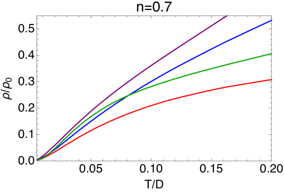
Figure 1: Resistivity plots for density 0.7 to T=0.2. Here the resistivity $\rho_{0}$ is defined [27] (see Eq. (40)) as the inverse of the characteristic conductivity $\sigma_{0}=e^{2}\hbar\Phi(0)/D$, with $\Phi(0)=\frac{1}{a_{0}^{3}}\rho_{DOS}(0)\langle(v_{k}^{x})^{2}\rangle_{\varepsilon_{k}=0}$ and $a_{0}$ the lattice constant. The red plots are second order with the $u_{0}$ sum rule, the blue are third order with the $u_{0}$ sum rule, the green are the DMFT results (using an extrapolation from higher density results) and the purple are second order without the $u_{0}$ sum rule using the Tukey window scheme. In this and other subsequent plots the DMFT results were kindly provided by Professor Rok Žitko.

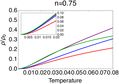
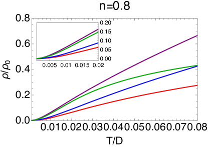
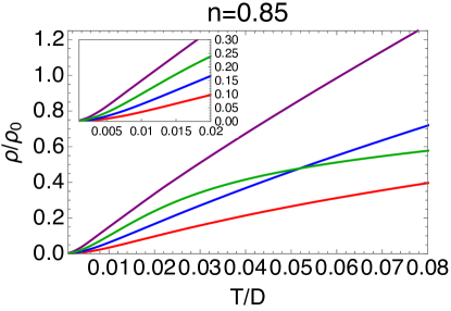
Figure 2: Resistivity plots for densities 0.75, 0.8 and 0.85. The resistivity $\rho_{0}$ is defined in the caption of Fig. (1). The red plots are second order with the $u_{0}$ sum rule, the blue are third order with the $u_{0}$ sum rule, the green are the DMFT results and the purple are second order without the $u_{0}$ sum rule using the Tukey window scheme. The insets show the resistivity on a smaller temperature scale.

In Fig. (2) we compare the resistivities obtained from the second order scheme (red), the third order scheme (blue), the Tukey window scheme (purple), and the exact DMFT results (green) at higher electron densities $n$, i.e. lesser hole doping $\delta=1-n$. The insets show the comparison at very low $T\ {\raise-2.15277pt\hbox{$\buildrel<\over{\sim}$}}\ 0.02D$ and the main figures present a larger regime $0\leq T\leq 0.08D$. In going from second to third order, we see that the resistivities are closer to the DMFT results at all densities. The Tukey window scheme on the other hand, is quite close to DMFT for $n<0.85$, while for $n=0.85$ it becomes an overcorrection.

In Fig. (3) we display the second chemical potential $u_{0}$ in the second and third order results and compare those with the Tukey window scheme results. Results are shown only up to $n=0.85$ since upon going past this limit, the third order $u_{0}$ grows beyond $\sim 4D$ rendering the convergence of the scheme as somewhat unstable.

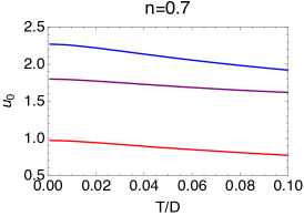
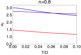
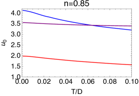
Figure 3: The second chemical potential $u_{0}$ (see Sec. 2.3) for densities 0.7, 0.8 and 0.85. The red plots are second order with the $u_{0}$ sum rule, the blue are third order with the $u_{0}$ sum rule and the purple are second order without the $u_{0}$ sum rule using the Tukey window scheme.

In Fig. (4) we display the imaginary part of the Dyson self energy $\rho_{\Sigma}(\omega)=-\frac{1}{\pi}\mathrm{Im}\Sigma(\omega)$ at low temperature ($T=0.001$D). In Fig. (5) these results are shown over a smaller energy scale $|\omega|\leq 0.1$D highlighting the lowest lying excitations of the electrons. Our results show a Fermi liquid type quadratic shape near zero frequency that lines up well with DMFT results. Note that these plots display spectral asymmetry between particle and hole type excitations, as previously discussed [32, 26].

In Fig. (4) we observe a pronounced peak in the DMFT self energy for the somewhat high energy excitations $\omega\sim-0.2$D. This peak is missing in all of our ECFL estimates. As a consequence the DMFT electron spectral functions $\rho_{\cal G}(k,\omega)$ in Eq. (12) are more compact in $\omega$ than any of the ECFL estimates on the $\omega<0$ (i.e. occupied) side.

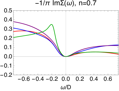
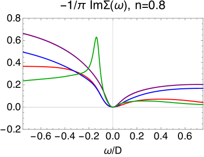
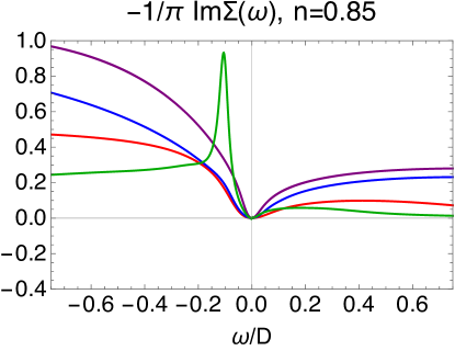
Figure 4: The imaginary part of the Dyson self energy for densities 0.7, 0.8 and 0.85, at T=0.001D. The red plots are second order with the $u_{0}$ sum rule, the blue are third order with the $u_{0}$ sum rule, the green are the DMFT results and the purple are second order without the $u_{0}$ sum rule using the Tukey window scheme.

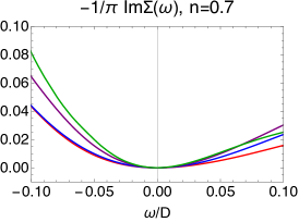
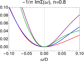
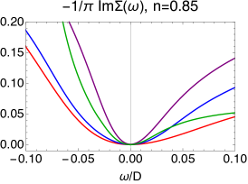
Figure 5: Spectral function plots for densities 0.7, 0.8 and 0.85, at T=0.001D for a smaller frequency range. The red plots are second order with the $u_{0}$ sum rule, the blue are third order with the $u_{0}$ sum rule, the green are the DMFT results and the purple are second order without the $u_{0}$ sum rule using the Tukey window scheme.

The quasiparticle weight $Z$ is obtainable from the self energy as $Z=\{1-\frac{\partial}{\partial\omega}\mathrm{Re}\Sigma(\omega)\}^{-1}$. The strong correlation physics problem usually leads to fragile quasiparticles, i.e. $Z\ll 1$ in the proximity of the Mott-Hubbard insulator at $\delta=0$. The reduction of its magnitude (from unity for the Fermi gas) is of especial interest, since it is one of the primary causal agents for the unusual transport and spectral properties in strongly correlated matter. The calculated $Z$ is displayed in Fig. (6) as a function of the hole density ($\delta=1-n$) and is seen to be $\ll 1$ as $\delta\leq 0.25$. The Z from our calculations compares quite well to the DMFT results. As noted earlier [26], the latter are well fit by $Z\sim\delta^{1.39}$. The third order $u_{0}$ sum rule results are closer to the DMFT results for Z than the second order results at all densities, and both of these overestimate the $Z$ for $\delta\leq 0.25$. In comparison the Tukey window scheme results are closer to the DMFT results but underestimate $Z$ for $\delta\leq 0.25$. As in the case of the resistivity, the Tukey scheme becomes an overcorrection at $\delta=0.15$.

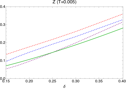
Figure 6: Z for densities 0.7-0.85 ($\delta$ 0.15-0.3).The red plots are second order with the $u_{0}$ sum rule, the blue are third order with the $u_{0}$ sum rule, the green are the DMFT results which fit well to $Z=\delta^{1.39}$[26], and the purple are second order without the $u_{0}$ sum rule using the Tukey window schemes.

5 Concluding Remarks

The ECFL theory has been developed so far using the ${\cal O}(\lambda)$ expressions for the self energies in the problem, and applied in a variety of situations including $d=0$ i.e. the Anderson Impurity model, the $d=1$  $t$-$J$  model, the $d=\infty,U=\infty$ Hubbard model and closest to experiments, the $d=2$  $t$-$J$  model. At a formal level we have also established a systematic method for extending the expansion to high order terms, but in view of the additional technical difficulties presented by them, these have not yet been tested. This work reports the first results from the third order equations for the ECFL, applied to the case of the $d=\infty$ and $U=\infty$ Hubbard model, where independent DMFT results are available from the numerical renormalization group. This enables us to quantify the role of the third order terms, and to compare with the second order results.

The introduction of an exact sum-rule for the  $t$-$J$  model allows us to bypass the somewhat ad-hoc Tukey window cutoff scheme used in previous ECFL resistivity computations [27, 18, 19]. In both the case of the second and third order results, the resistivity curve from ECFL agrees in both shape and scale with the one from DMFT, with a quadratic in temperature Fermi-liquid regime, followed by a quasi-linear strange-metal regime. Both ECFL and DMFT predict a monotonic decrease in the quasi-particle weight as one approaches half-filling. In both the case of resistivity and quasi-particle weight, third order ECFL improves upon the second order ECFL at all densities, in comparison to DMFT. The Tukey scheme constitutes a further correction at lower densities, but at higher densities it constitutes and over-correction, overshooting the DMFT results. Finally, both ECFL and DMFT find the quadratic quasi-particle minimum in the Dyson self-energy at low frequencies, while DMFT has a higher (negative) frequency peak, which is absent from the low-order ECFL results. It is encouraging that in going from second to third order in the ECFL computation we obtain better agreement with DMFT.

6 Acknowledgements

We are grateful to Professor Rok Žitko for permitting us to use the results of his dynamical mean field theory calculations of the $d=\infty$ and $U=\infty$ data for comparison with our results. The work at UCSC was supported by the US Department of Energy (DOE), Office of Science, Basic Energy Sciences (BES), under Award No. DE-FG02-06ER46319. The computation was done on the comet in XSEDE[33] (TG-DMR170044) supported by National Science Foundation grant number ACI-1053575.

Appendix A Appendix: The second sum rule

We give a brief derivation of the sum-rule valid in infinite dimensions

$$\sum_{k}\int d\omega\rho_{{\cal G}}(k,\omega)f(\omega)(\omega+{\bm{\mu}}-\varepsilon_{k})=0.$$ (48)

We start with the Hamiltonian (energy minus ${\bm{\mu}}N$) written in terms of the Hubbard operators[3, 4]

$$H=-\sum_{i,j,\sigma}t_{ij}X_{i}^{\sigma 0}X_{j}^{0\sigma}-{\bm{\mu}}\sum_{i,\sigma}X_{i}^{\sigma\sigma}+\frac{1}{2}\sum_{i,j}J_{ij}(\vec{S}_{i}\cdot\vec{S}_{j}-\frac{1}{4}n_{i}n_{j})$$ (49)

We rewrite this in the form

$$=-\sum_{i,j,\sigma}t_{ij}X_{i}^{\sigma 0}X_{j}^{0\sigma}-{\bm{\mu}}\sum_{i,\sigma}X_{i}^{\sigma\sigma}+V_{ex}$$ (50)

where the exchange energy is

$$V_{ex} = -\frac{1}{4}\sum_{ij\sigma\sigma^{\prime}}\sigma\sigma^{\prime}J_{ij}X_{i}^{\sigma\sigma^{\prime}}X_{j}^{\bar{\sigma}\bar{\sigma}^{\prime}}$$ (51)

$$= \frac{1}{4}\sum_{ij,\sigma}J_{ij}(X_{i}^{\sigma\bar{\sigma}}X_{j}^{\bar{\sigma}\sigma}-X_{i}^{\sigma\sigma}X_{j}^{\bar{\sigma}\bar{\sigma}})$$

and define the electron Green’s function

$${\cal G}_{\sigma_{i}\sigma_{f}}(i\tau_{i},f\tau_{f})=-\frac{1}{Z_{G}}\mathrm{Tr}\,e^{-\beta H}T_{\tau}\left(X_{i}^{0\sigma_{i}}(\tau_{i})X_{f}^{\sigma_{f}0}(\tau_{f})\right)$$ (52)

where $Z_{G}=\mathrm{Tr}\,e^{-\beta H}$. Taking the time derivative with respect to $\tau_{i}$ and then setting $\tau_{f}=\tau_{i}+0^{+}$, $\sigma_{i}=\sigma_{f}=\sigma$ and the sites $i=f$ we get

$$\partial_{\tau_{i}}{\cal G}_{\sigma\sigma}(i,i^{+})={\bm{\mu}}\langle X_{i}^{\sigma\sigma}\rangle+\sum_{j}t_{ij}\langle X_{i}^{\sigma 0}X_{j}^{0\sigma}\rangle+\frac{1}{2}\sum_{j\sigma^{\prime}}J_{ij}\sigma\sigma^{\prime}\langle X_{i}^{\sigma\sigma^{\prime}}X_{j}^{\bar{\sigma}\bar{\sigma}^{\prime}}\rangle$$ (53)

where we dropped a term containing $\delta(\tau_{i}-\tau_{f})$ (since we are considering the limit $\tau_{f}=\tau_{i}+0^{+}$). Summing over $\sigma$, denoting $\tau=\tau_{i}-\tau_{f}$, and summing over site index $i$ (replaced by a $\vec{k}$ sum), we get

$$2\partial_{\tau}\sum_{\vec{k}}{\cal G}(\vec{k},\tau)\bigg{|}_{\tau\to 0^{-}}={\bm{\mu}}N-\langle T\rangle-2\langle V_{ex}\rangle.$$ (54)

It is convenient to introduce the general formula for the Greens function in terms of the spectral function in time domain

$${\cal G}(\vec{k},\tau)=\int\,d\nu\,\rho_{{\cal G}}(\vec{k},\nu)\,e^{-\nu\tau}\left(f(\nu)\Theta(-\tau)-\bar{f}(\nu)\Theta(\tau)\right),$$ (55)

where $f$ is the fermi function and $\bar{f}=1-f$, and $\Theta(\tau)$ is the Heaviside theta function. Substituting into Eq. (54) and transposing terms we get

$$-2\sum_{\vec{k}}\int\,d\nu\,\nu\,\rho_{{\cal G}}(\vec{k},\nu)-{\bm{\mu}}N+\langle T\rangle=-2\langle V_{ex}\rangle$$ (56)

Using $2\sum_{\vec{k}}\int\,d\nu\,\,\rho_{{\cal G}}(\vec{k},\nu)=N$ and $2\sum_{\vec{k}}\int\,d\nu\,\varepsilon_{k}\,\rho_{{\cal G}}(\vec{k},\nu)=\langle T\rangle$, we get

$$\sum_{k}\int d\omega\rho_{{\cal G}}(k,\omega)f(\omega)(\omega+{\bm{\mu}}-\varepsilon_{k})=\langle V_{ex}\rangle.$$ (57)

In $d=\infty$ we set $J=0$ and hence $V_{ex}$ vanishes and we get the sum-rule Eq. (48).

In lower dimensions we are obliged to use some suitable approximation to estimate $\langle V_{ex}\rangle$. In the physically important case relevant to cuprates of $d=2$ on a square lattice (with 4 neighbors), we may use a Hartree type approximation

$$\langle V_{ex}\rangle=-\frac{1}{4}\sum_{ij\sigma\sigma^{\prime}}\sigma\sigma^{\prime}J_{ij}\langle X_{i}^{\sigma\sigma^{\prime}}X_{j}^{\bar{\sigma}\bar{\sigma}^{\prime}}\rangle\sim-\frac{1}{4}\sum_{ij\sigma}J_{ij}\langle X_{i}^{\sigma\sigma}\rangle\langle X_{j}^{\bar{\sigma}\bar{\sigma}}\rangle=-\frac{n^{2}}{8}N_{s}Z_{c}J,$$ (58)

where $J$ is the nearest neighbor exchange energy and $Z_{c}$ is the number of nearest neighbors in the lattice.

Appendix B Appendix: Program Notes

Our program at both second and third order uses a rootfinder with two equations and two variables to solve for ${\bm{\mu}}^{\prime}$and $u_{0}$. We use Eq. (45, 43) as mentioned in the text. We noted that the third order program is significantly more stable with this choice of sum-rules.

It is generally true that, whichever two sumrules are chosen, the third will be approximately satisfied. Since the $n_{G}$ rule and new $u_{0}$ sumrule are used, $n_{G}$ is exactly equal to $n$, while $n_{g}$ is only approximately equal to $n$. As mentioned previously, the $n_{g}$ value generally ends up $10$ to $15$% higher than $n$. When used in Eq. (28), the different value of $n_{g}$ can cause noise under iteration, resulting in a failure to converge. This effect is particularly pronounced for the $O(\lambda^{3})$ program. So we approximate $n_{g}$ with $n$ in our chemical potential (Eq. (29)), which gives very similar results in all well behaved cases we compared. It should be noted that multiplying $n$ by a constant to bring it closer to $n_{g}$ also causes failure to converge at third order; for best results the $n$ approximation should be used.

Here we would also like to outline the parameters under which our programs are well behaved. The $O(\lambda^{2})$ program converges with relative ease for a wide range of temperatures and densities. We tested densities around 0.5-0.9 and temperatures from 0.001 to 0.2 with good results. The $O(\lambda^{2})$ program also functions well with the $n_{g}$ sumrule substituted for the $n_{G}$ sumrule.

The third order program is generally more unstable than second order. It converges comfortably for densities 0.7-0.85 over our full temperature range, 0.001-0.02. Beyond those densities the program rapidly becomes more difficult to run. For lower densities it is possible to push the program to converge a little below 0.6. For higher densities in particular the third order program consistently has significant difficultly converging. We recommend this technique not be extended beyond optimal density (0.85).

References

- [1] M. C. Gutzwiller, Phys. Rev. Letts.,10, 159 (1963), J. Hubbard, Proc. R. Soc. London A 276, 238 (1963), J. Kanamori, Prog. Theor. Phys. 30 275 (1963).
- [2] A. B. Harris and R. V. Lange, Phys. Rev. 157, 295 (1967).
- [3] B. S. Shastry, Phys. Rev. Letts. 107, 056403 (2011); Phys. Rev. B 87, 125124 (2013).
- [4] B. S. Shastry, Phys. Rev. B 87, 125124 (2013).
- [5] B. S. Shastry, Ann. Phys. 343, 164-199 (2014).
- [6] A. Georges, G. Kotliar, W. Krauth and M. J. Rozenbereg, Rev. Mod. Phys. 68, 13 (1996).
- [7] X. Deng, J. Mravlje, M. Ferrer, G. Kotliar, A.Georges, Phys. Rev. Letts. 110, 086401 (2013).
- [8] W. Xu, K. Haule, and G. Kotliar, Phys. Rev. Letts. 111, 036401 (2013).
- [9] W. Wu, X. Wang, and A. Tremblay, arXiv preprint arXiv:2109.02635 (2021).
- [10] E. W. Huang et al., Science 366, 987-990 (2019) .
- [11] K. Held, Adv. in Phys. 56, 829 (2007).
- [12] W. Metzner and D. Vollhardt, Phys. Rev. Lett. 62, 324 (1989).
- [13] S. Biermann, F. Aryasetiawan and A. Georges, Phys. Rev. Letts. 90, 086401 (2003).
- [14] K. G. Wilson, Rev. Mod. Phys. 47, 773 (1975).
- [15] H. R. KrishnaMurthy, J. W. Wilkons and K. G. Wilson, Phys. Rev. B 21, 1003 (1980).
- [16] R. Žitko, H. R. Krishnamurthy and B. S. Shastry, Phys. Rev. B 98, 161121(R) (2018); B. S. Shastry, E. Perepelitsky and A. C. Hewson, Phys. Rev. B 88, 205108 (2013).
- [17] P. Mai, S. R. White and B. S. Shastry, Phys. Rev. B 98, 035108 (2018).
- [18] W. Ding, R. Žitko, and B. S. Shastry, Phys. Rev. B 96, 115153 (2017).
- [19] W. Ding, R. Žitko, P. Mai, E. Perepelitsky and B. S. Shastry Phys. Rev. B 96, 054114 (2017).
- [20] B. S. Shastry and P. Mai, Phys. Rev. B101, 115121 (2020).
- [21] P. Mai and B. S. Shastry, Phys. Rev. B98, 205106 (2018).
- [22] B S. Shastry and P. Mai, New Jour. Phys. 20 013027 (2018).
- [23] B. S. Shastry, Ann. Phys. 343, 164-199 (2014). (Erratum) Ann. Phys. 373, 717-718 (2016).
- [24] E. Perepelitsky and B. S. Shastry, Ann. Phys. 357, 1 (2015).
- [25] E. Perepelitsky and B. S. Shastry, Ann. of Physics 338, 283-301 (2013).
- [26] R. Žitko, D. Hansen, E. Perepelitsky, J. Mravlje, A. Georges and B. S. Shastry, Phys. Rev. B 88, 235132 (2013).
- [27] B. S. Shastry, E. Perepelitsky, Phys. Rev. B 94, 045138 (2016).
- [28] F. J. Dyson, Phys. Rev. 102, 1217 (1956).
- [29] S. V. Maleev, Sov. Phys. JETP 6, 776 (1958).
- [30] These follow from Eq. (7,8,9) of [27], where we replaced by using the number sumrule Eq. (43) for the physical particles.
- [31] This sum-rule is a consequence of the fall off of (see Eq. (5), and ).
- [32] B. S. Shastry, Phys. Rev. Letts. 109, 067004 (2012).
- [33] J. Town et al., Computing in Science & Engineering, Vol.16, No. 5, pp. 62-74, Sept.-Oct. 2014.