Dynamical systems defined on simplicial complexes: symmetries, conjugacies, and invariant subspaces

Abstract

We consider the general model for dynamical systems defined on a simplicial complex. We describe the conjugacy classes of these systems and show how symmetries in a given simplicial complex manifest in the dynamics defined thereon, especially with regard to invariant subspaces in the dynamics.

Lead Paragraph: In this paper we study the general form of a nonlinear dynamical system defined on a simplicial complex, which is a natural higher-order generalization of dynamics on a network. We first show that many of the important algebraic homological structures survive when we consider nonlinear systems. We give a full description of the conjugacy class of dynamical systems that can be defined on a simplicial complex, and also give a process by which one can construct a system on a given complex that is equivalent to any given dynamical system. We show that the choice of orientation matters for simplicial complexes and understand the impact of changing orientations, and finally we study the (dynamical) symmetries of dynamical systems defined on simplicial complexes that have their own (algebraic) symmetries.

1 Introduction

1.1 Background

The field of network science has grown significantly over the last few decades [34, 10, 3, 33], but more recently, in just the last few years, there has been significant activity in both the modeling and empirical communities that we should not just consider pairwise interactions, but we should also pay attention to interactions of larger subsets of elements [41, 31, 27, 47, 43, 16, 5, 13, 44, 24, 25, 26, 40, 12, 38, 23, 30, 46, 7, 4, 1]. For very nice and comprehensive surveys of the state of the art, see [6, 39, 9]. Another way of saying this is that we should not just consider dynamics on graphs but also on hypergraphs [8, 11]. A special subclass of hypergraphs is the simplicial complexes; these are hypergraphs with the property that if a subset is active, then all of its subsets are also active. These are the structures we discuss in this paper. The study of simplicial complexes has a long history in mathematics [32, 21, 28] and underpins many modern tools in algebraic topology and homological algebra.

In some form or another, the main question from the field of network dynamical systems asks how a network structure influences dynamical behavior. Some of the most successful approaches consist of identifying some combinatorial or algebraic structure in a given network, and translating this structure into necessary geometric features of the dynamics. Notable in this respect is the groupoid formalism of Golubitsky, Stewart et al [45, 19, 17], which allows one to predict robust synchrony patterns, among other dynamical properties. Another clear example is the translation of a symmetry in the network graph into a symmetry of the corresponding dynamical system [18, 15]. Other methods use graph-fibrations [14, 35] and generalized or hidden symmetries [2, 36, 37].

The main questions that we would like to answer in this paper are:

1. What is the most general framework for (ODE) dynamics that can be said to be consistent with a simplicial complex structure?

2. When the dynamics live on a simplicial complex, and this complex has certain algebraic symmetries, what does this imply for the {symmetries/quasi-symmetries/etc.} of the dynamics?

Finally, the main point: we seek to do for simplicial dynamics what previous authors have done for network dynamics.

Towards this goal, we will first show that the linear structure that is commonly used in homological and cohomological computations both survives in, and is important in understanding, the ODE models on simplicial complexes (Section 2). We then investigate the conjugacy classes of dynamical systems on a specific simplicial complex (Sections 3, 4), the impact of choices of orientation on these dynamical systems (Section 5), and finally finish with a study of the symmetries and invariant spaces of dynamical systems on simplicial complexes (Sections 6 7).

1.2 General model definition

As described above, we present the general definition of the flow we study.

Definition 1.1 (Simplicial complex).

Let $V$ be a set. A $k$-simplex is a unordered set $\{v_{0},\dots,v_{k}\}$ with $v_{i}\in V$ and $v_{i}\neq v_{j}$ if $i\neq j$. A face of a $k$-simplex is all $(k-1)$-simplices of the form $\{v_{0},\dots,v_{k}\}\setminus\{v_{i}\}$, which we will also denote by $\{v_{0},\dots,\widehat{v_{i}},\dots,v_{k}\}$. A simplicial complex $X$ is a collection of simplices closed under inclusion of all faces, and we denote by $X_{d}$ the set of simplices that contain precisely $d+1$ elements. We will also say that the simplices in $X_{d}$ are of dimension $d$. We denote by $d_{{\mathsf{max}}}(X)$ the maximal dimension of all of the simplices in $X$.

Two $d$-simplices $F_{1},F_{2}$ of a complex $X$ are called upper adjacent if both are faces of some $d+1$-simplex; in this case we write $F_{1}\smallfrown F_{2}$. Two $d$-simplices $F_{1},F_{2}$ of a complex $X$ are called lower adjacent if they have a common face; in this case we write $F_{1}\smallsmile F_{2}$.

An ordering of vertices gives an orientation, and an oriented $k$-simplex is a $k$-simplex with an order type. By definition, orientation is anti-symmetric with respect to an exchange of vertices. We denote an ordered simplex by square brackets, e.g. $[v_{0},\dots,v_{k}]$. $\triangle$

For $X$ a simplicial complex, let $C_{d}(X)$ be the $\mathbb{R}$-vector space with basis given by the elements of $X_{d}$. For each $d$, we have the boundary map defined by

$$\partial_{d}\colon C_{d}(X) \to C_{d-1}(X)$$

$$[v_{0},\dots,v_{d}] \mapsto\sum_{\ell=0}^{d}(-1)^{\ell}[v_{0},\dots,\widehat{v_{\ell}},\dots,v_{d}]$$

and extended by linearity. (As is well known, the map $\partial_{d}\circ\partial_{d+1}$ is identically zero.) The elements of the kernel of the map $\partial_{d}\colon C_{d}(X)\to C_{d-1}(X)$ are known as the $d$-cycles of the complex $X$, and the image of $\partial_{d+1}\colon C_{d+1}(X)\to C_{d}(X)$ consists of the $d$-boundaries. Since $\partial_{d}\circ\partial_{d+1}=0$, it is natural to define the $d$-th homology group $H_{d}(X):=\ker\partial_{d}/\operatorname{Im}\partial_{d+1}$. There is also a natural inner product on $C_{d}(X)$; with respect to this inner product we can define the adjoint map $\partial^{*}_{d}\colon C_{d-1}(X)\to C_{d}(X)$. We also define the $d$-cocyles as $\ker(\partial^{*}_{d+1})$ and $d$-coboundaries as $\operatorname{Im}(\partial^{*}_{d})$.

Choosing an ordering of the elements of $X_{d}$ naturally chooses an ordered basis for $C_{d}(X)$. With this ordered basis we can define the matrix $B_{d}$ to be the matrix representation of $\partial_{d}$. We assume implicitly in all that follows that such an ordering has been chosen and fixed for $X_{d}$.

The most general ODE we will consider here in this paper is given by

$$\frac{d}{dt}\theta_{d}=G^{0}_{d}(\theta_{d})+B_{d}^{\intercal}F^{\downarrow}_{d}(B_{d}\theta_{d})+B_{d+1}F^{\uparrow}_{d}(B_{d+1}^{\intercal}\theta_{d})\,$$ (1)

where

$$F^{\downarrow}_{d}\colon C_{d-1}(X)\to C_{d-1}(X),\quad F^{\uparrow}_{d}\colon C_{d+1}(X)\to C_{d+1}(X)$$

can be arbitrary nonlinear functions. The function $G^{0}_{d}$ satisfies the condition that the $i$th coordinate of $G^{0}_{d}$ depends only on the $i$th coordinate of its input. We will write

$$G^{\downarrow}_{d}:=B_{d}^{\intercal}F^{\downarrow}_{d}B_{d},\quad G^{\uparrow}_{d}=B_{d+1}F^{\uparrow}_{d}B_{d+1}^{\intercal},\quad G_{d}:=G^{\downarrow}_{d}+G^{\uparrow}_{d},$$

thus giving the more compact description of (1):

$$\frac{d}{dt}\theta_{d}=G^{0}_{d}(\theta_{d})+G^{\downarrow}_{d}(\theta_{d})+G^{\uparrow}_{d}(\theta_{d}).$$ (2)

The main motivation behind this form of equation is that each of the terms represents a different type of interaction. The first term, $G_{d}^{0}(\cdot)$, represents “internal dynamics”: we allow a simplex to depend on its own value. The next term, $G^{\uparrow}_{d}(\cdot)$, represents an “up-coupling”: each simplex depends on the others only through couplings via a higher-dimensional simplex, and similarly for the “down-coupling”.

Finally, although we allow for general nonlinear functions $F^{\downarrow}_{d}$ and $F^{\uparrow}_{d}$ in (1), we often consider one class of functions in particular, defined as:

Definition 1.2.

We call $f\colon\mathbb{R}^{n}\to\mathbb{R}^{n}$ a componentwise function if the $k$th component function of $f$ is a function only of the $k$th variable, i.e. if

$$f_{k}(x_{1},\dots,x_{n})=f_{k}(x_{k}).$$

Note that $G^{0}_{d}$ is assumed componentwise above, and we will see that we can obtain some strong results when $F^{\uparrow}_{d}$ and $F^{\downarrow}_{d}$ are assumed to be componentwise. $\triangle$

2 The triple decomposition

In this section we present a natural “triple decomposition” of the space $C_{d}(X)$. This decomposition is standard, but here we show that it naturally interacts well with the nonlinear flow.

Definition 2.1.

We denote $W_{d}:=\ker(B_{d})\cap\ker(B_{d+1}^{\intercal})\subseteq C_{d}(X)$. $\triangle$

Lemma 2.2.

For all $d$ we have the orthogonal decomposition

$$C_{d}(X)=\operatorname{Im}(B_{d}^{\intercal})\oplus\operatorname{Im}(B_{d+1})\oplus W_{d},$$ (3)

which we refer to as the triple decomposition below. We also have

$$\ker(B_{d})=\operatorname{Im}(B_{d+1})\oplus W_{d},\quad\ker(B_{d+1}^{\intercal})=\operatorname{Im}(B_{d}^{\intercal})\oplus W_{d}$$

from which we obtain the useful orthogonal decompositions

$$C_{d}(X) =\operatorname{Im}(B_{d}^{\intercal})\oplus\ker(B_{d}),$$ (4)

$$C_{d}(X) =\operatorname{Im}(B_{d+1})\oplus\ker(B_{d+1}^{\intercal}).$$ (5)

Remark 2.3.

We leave the proof of 2.2 to Appendix A, but note that all of these statements follow from two observations: the Rank–Nullity theorem, plus the fact that $B_{d}B_{d+1}=0$.

Definition 2.4.

We denote by $P_{d}$, $Q_{d}$ and $R_{d}$ the orthogonal projections onto $\operatorname{Im}(B_{d}^{\intercal})$, $\operatorname{Im}(B_{d+1})$ and $W_{d}$, respectively in the triple decomposition (3). It follows directly from Lemma 2.2 that $P_{d}+Q_{d}+R_{d}=I_{d}:=\operatorname{Id}_{C_{d}(X)}$. We also see that the pair of projections $(P_{d},I_{d}-P_{d})$ gives the decomposition (4), and the pair $(Q_{d},I_{d}-Q_{d})$ gives the decomposition (5). $\triangle$

It follows directly from the definitions above that $P_{d}B_{d}^{\intercal}=B_{d}^{\intercal}$ and $Q_{d}B_{d+1}=B_{d+1}$. We also note that since the projections are orthogonal, they are self-adjoint as operators, and from this $B_{d}P_{d}=B_{d}$ and $B_{d+1}^{\intercal}Q_{d}=B_{d+1}^{\intercal}$. This means that

$$G^{\uparrow}_{d}=B_{d+1}F^{\uparrow}_{d}B_{d+1}^{\intercal}=B_{d+1}(P_{d+1}F^{\uparrow}_{d}P_{d+1})B_{d+1}^{\intercal}.$$ (6)

(Of course, the analogous argument applies, mutatis mutandis, for $F^{\downarrow}_{d}$ and $Q_{d-1}$.) We formalize this:

Definition 2.5.

Consider the space of all smooth maps from $C_{d}(X)$ to itself. We define two equivalence relations on this set: $\sim^{\uparrow}_{d},\sim^{\downarrow}_{d}$, defined by

$$\mathcal{A}\sim^{\uparrow}_{d}\mathcal{B} \iff P_{d}\mathcal{A}P_{d}=P_{d}\mathcal{B}P_{d},$$

$$\mathcal{A}\sim^{\downarrow}_{d}\mathcal{B} \iff Q_{d}\mathcal{A}Q_{d}=Q_{d}\mathcal{B}Q_{d}.$$

$\triangle$

Lemma 2.6.

There is a one-to-one correspondence between the equivalence classes of $\sim^{\uparrow}_{d+1}$ and distinct maps of the form $G^{\uparrow}_{d}=B_{d+1}F^{\uparrow}_{d}B_{d+1}^{\intercal}$, and the bijection is realized by the map $[F^{\uparrow}_{d}]\mapsto B_{d+1}F^{\uparrow}_{d}B_{d+1}^{\intercal}$.

Similarly, there is a one-to-one correspondence between the equivalence classes of $\sim^{\downarrow}_{d-1}$ and distinct maps of the form $G^{\downarrow}_{d}=B_{d}^{\intercal}F^{\downarrow}_{d}B_{d}^{\intercal}$, and the bijection is realized by the map $[F^{\downarrow}_{d}]\mapsto B_{d}^{\intercal}F^{\downarrow}_{d}B_{d}^{\intercal}$.

Proof.

We will prove the statement for $\sim^{\uparrow}_{d+1}$, and the second is similar.

It is clear from (6) that $\mathcal{A}\sim^{\uparrow}_{d+1}\mathcal{B}$ implies $B_{d+1}\mathcal{A}B_{d+1}^{\intercal}=B_{d+1}\mathcal{B}B_{d+1}^{\intercal}$. Now, assume that $\mathcal{A},\mathcal{B}$ satisfy $B_{d+1}\mathcal{A}B_{d+1}^{\intercal}=B_{d+1}\mathcal{B}B_{d+1}^{\intercal}$. Define $\mathcal{C}=\mathcal{A}-\mathcal{B}$, and then $B_{d+1}\mathcal{C}B_{d+1}^{\intercal}=0$. Using (6) again, we see that $B_{d+1}P_{d+1}\mathcal{C}P_{d+1}B_{d+1}^{\intercal}=0$ as well. Now, Lemma 2.2 tells us that

$$C_{d+1}(X)=\operatorname{Im}(B_{d+1}^{\intercal})\oplus\ker(B_{d+1})=\operatorname{Im}(P_{d+1})\oplus\ker(B_{d+1}),$$

so that $B_{d+1}$ is injective on $\operatorname{Im}(P_{d+1})$. It follows that $P_{d+1}\mathcal{C}P_{d+1}B_{d+1}^{\intercal}=0$, so that $P_{d+1}\mathcal{C}P_{d+1}$ vanishes on $\operatorname{Im}(B_{d+1}^{\intercal})=\operatorname{Im}(P_{d+1})$. As $P_{d+1}$ is a projection, we conclude that

$$P_{d+1}\mathcal{C}P_{d+1}=P_{d+1}\mathcal{C}P_{d+1}^{2}=(P_{d+1}\mathcal{C}P_{d+1})|_{\operatorname{Im}(P_{d+1})}P_{d+1}=0.$$

This implies $P_{d+1}\mathcal{A}P_{d+1}=P_{d+1}\mathcal{B}P_{d+1}$ and thus $\mathcal{A}\sim^{\uparrow}_{d+1}\mathcal{B}$. ∎

Consider the decomposition of $C_{d+1}(X)$ generated by the pair of projections $(P_{d+1},I_{d+1}-P_{d+1})$; writing $\theta_{d+1}=(x,y):=(P_{d+1}\theta_{d+1},(I_{d+1}-P_{d+1})\theta_{d+1})$ and $F^{\uparrow}_{d}=(g,h):=(P_{d+1}F^{\uparrow}_{d},(I_{d+1}-P_{d+1})F^{\uparrow}_{d})$, then generally we have

$$F^{\uparrow}_{d}=\begin{pmatrix}g(x,y)\\ h(x,y)\end{pmatrix},\quad P_{d+1}F^{\uparrow}_{d}P_{d+1}=\begin{pmatrix}g(x,0)\\ 0\end{pmatrix}\,.$$

From (6) we see that these “versions” of $F^{\uparrow}_{d}$ will give the same $G^{\uparrow}_{d}$, and so far as we are concerned they are equivalent. Clearly, the function with the projections is simpler, and we would like to use it as a canonical representative of all $F^{\uparrow}_{d}$ that give the same vector field, giving the following definition:

Definition 2.7.

The canonical representative of an equivalence class $[\mathcal{A}]$ for $\sim^{\uparrow}_{d}$ is the function $P_{d}\mathcal{A}P_{d}$;
the canonical representative of an equivalence class $[\mathcal{A}]$ for $\sim^{\downarrow}_{d}$ is the function $Q_{d}\mathcal{A}Q_{d}$. $\triangle$

Remark 2.8.

Note that there is a one-to-one correspondence between equivalence classes of $\sim^{\uparrow}_{d+1}$ and maps from $\operatorname{Im}(B_{d+1}^{\intercal})$ to itself. More precisely, to a map $f:\operatorname{Im}(B_{d+1}^{\intercal})\rightarrow\operatorname{Im}(B_{d+1}^{\intercal})$ we may associate the class under $\sim^{\uparrow}_{d+1}$ of

$$F^{\uparrow}_{d}=\begin{pmatrix}f(x)\\ 0\end{pmatrix}:C_{d+1}(X)\rightarrow C_{d+1}(X)\,,$$ (7)

where the two components of the vector correspond to the decomposition

$$C_{d+1}(X)=\operatorname{Im}(B_{d+1}^{\intercal})\oplus\ker(B_{d+1})\,.$$

This bijectively sends the maps $f:\operatorname{Im}(B_{d+1}^{\intercal})\rightarrow\operatorname{Im}(B_{d+1}^{\intercal})$ to the canonical representatives for $\sim^{\uparrow}_{d+1}$. Likewise, there is a correspondence between equivalence classes of $\sim^{\downarrow}_{d-1}$ and maps from $\operatorname{Im}(B_{d})$ to itself, by sending a map $g:\operatorname{Im}(B_{d})\rightarrow\operatorname{Im}(B_{d})$ to the class under $\sim^{\downarrow}_{d-1}$ of

$$F^{\downarrow}_{d}=\begin{pmatrix}g(x)\\ 0\end{pmatrix}:C_{d-1}(X)\rightarrow C_{d-1}(X)\,,$$ (8)

where the two components correspond to the decomposition

$$C_{d-1}(X)=\operatorname{Im}(B_{d})\oplus\ker(B_{d}^{\intercal})\,.$$

This bijectively sends the maps $g:\operatorname{Im}(B_{d})\rightarrow\operatorname{Im}(B_{d})$ to the canonical representatives for $\sim^{\downarrow}_{d-1}$. In conclusion, even though $G^{\uparrow}_{d}$ and $G^{\downarrow}_{d}$ are both vector fields on $C_{d}(X)$, we see that they are uniquely determined by vector fields on $\operatorname{Im}(B_{d+1}^{\intercal})$ and $\operatorname{Im}(B_{d})$, respectively. $\triangle$

3 Realization of specific vector fields

A natural question arises: let us say that we have a particular vector field in mind, is it possible to realize it as a flow on a simplicial complex? More specifically, we would like to describe the conjugacy class of all vector fields of the form

$$\frac{d}{dt}\theta_{d}=B_{d}^{\intercal}F^{\downarrow}_{d}(B_{d}\theta_{d})+B_{d+1}F^{\uparrow}_{d}(B_{d+1}^{\intercal}\theta_{d}).$$ (9)

Also, we want to generate a process by which we can determine how to choose $F^{\uparrow}_{d},F^{\downarrow}_{d}$, to get the vector field we desire.

Definition 3.1 (Moore–Penrose psuedoinverse).

[22, Section 7.3] If $L\colon V\to W$ is a linear operator, then the linear operator $L^{+}\colon W\to V$ satisfying:

1. $LL^{+}L=L$;

2. $L^{+}LL^{+}=L^{+}$;

3. $LL^{+}$ and $L^{+}L$ are positive semi-definite.

is known as the Moore–Penrose psuedoinverse (or, more briefly, the psuedoinverse) of $L$. $\triangle$

Lemma 3.2.

For any $L\colon V\to W$, the pseudoinverse exists and is unique. Moreover, we have the following orthogonal decompositions:

$$V=\ker L\oplus\operatorname{Im}L^{+},\quad\quad W=\ker L^{+}\oplus\operatorname{Im}L.$$

Finally, $(L^{*})^{+}=(L^{+})^{*}$, and we write $L^{+*}$ to be either operator.

We prove this lemma below in Appendix A.

Remark 3.3.

By choosing a basis for $V$ and $W$, we can derive the analogous statements about matrices. $\triangle$

Definition 3.4.

Given a vector space $V$ and a decomposition $V=V_{1}\oplus V_{2}$, we say that $F\colon V\to V$ is independent of $V_{1}$ if, whenever $v=v_{1}+v_{2}$ with respect to the decomposition, we have $F(v)=F(v_{2})$. $\triangle$

Lemma 3.5.

Let $L\colon V\to W$ be a linear map and assume that $G\colon W\to W$ has the property that $G$ is independent of $\ker L^{*}$ with respect to the decomposition $W=\ker L^{*}\oplus\operatorname{Im}L^{+*}$, and $G(W)\subseteq\operatorname{Im}L$. Then there exists a function $F\colon V\to V$ such that $G(x)=LF(L^{*}x)$. More specifically, we can choose

$$F(y):=L^{+}G(L^{+*}y)$$ (10)

as such a function (although this is typically not the only choice that works).

Proof.

Since $G(W)\subseteq\operatorname{Im}L$, we can write $G(x)=L\mathcal{G}(x)$ for some function $\mathcal{G}$. Since $G$ is independent of $\ker L^{*}$, we can consider the decomposition $W=\ker L^{*}\oplus\operatorname{Im}L^{+*}$. If we let $x=x_{1}+x_{2}$ in this decomposition, then $G(x)=G(x_{2})$, and as such we can assume that the argument of $G$ lies in $\operatorname{Im}L^{+*}$. In summary, we can write $G(x)=L\mathcal{G}(L^{+*}y)$ for some $y\in V$.

Now assume the choice made in (10), and we compute

$$LF(L^{*}x)=LL^{+}G(L^{+*}L^{*}x)=LL^{+}L\mathcal{G}(L^{+*}L^{*}L^{+*}y)=L\mathcal{G}(L^{+*}y)=G(x).$$

∎

Proposition 3.6.

Let $G_{1}\colon\operatorname{Im}(B_{d}^{\intercal})\to\operatorname{Im}(B_{d}^{\intercal})$ and $G_{2}\colon\operatorname{Im}(B_{d+1})\to\operatorname{Im}(B_{d+1})$, then $G_{1}\oplus G_{2}\oplus{\bf 0}_{W_{d}}$ is the right-hand side of (9) for some choices of $F^{\uparrow}_{d},F^{\downarrow}_{d}$.

Proof.

Let us write $U_{d}=\operatorname{Im}(B_{d}^{\intercal})$ and $V_{d}=\operatorname{Im}(B_{d+1})$. For each of $G_{1},G_{2}$, we extend their domains. For $x\in C_{d}(X)$, write $x=x_{1}+x_{2}\in U_{d}\oplus U_{d}^{\perp}$, and define $\widetilde{G}_{1}(x):=G_{1}(x_{1})$. Similarly, for $y\in C_{d}(X)$, write $y=y_{1}+y_{2}\in V_{d}\oplus V_{d}^{\perp}$, and define $\widetilde{G}_{2}(x):=G_{2}(x_{2})$.

Note that $\widetilde{G}_{1}$ satisfies the assumptions of Lemma 3.5 for the linear operator given by $B_{d}^{\intercal}$; clearly $\widetilde{G}_{1}(C_{d}(X))\subseteq U_{d}$ by definition, and $U_{d}^{\perp}=(\operatorname{Im}(B_{d}^{\intercal}))^{\perp}=\ker B_{d}$. As such there is $F^{\downarrow}_{d}\colon C_{d-1}(X)\to C_{d-1}(X)$ giving $\widetilde{G}_{1}=B_{d}^{\intercal}F^{\downarrow}_{d}B_{d}$. The argument is similar for $\widetilde{G}_{2}$, which gives the result. ∎

Definition 3.7.

We call $H\colon\mathbb{R}^{n}\to\mathbb{R}^{n}$ an $(\alpha,\beta,n)$-vector field (for $\alpha+\beta\leq n$) if there exist $H_{1}\colon\mathbb{R}^{\alpha}\to\mathbb{R}^{\alpha}$ and $H_{2}\colon\mathbb{R}^{\beta}\to\mathbb{R}^{\beta}$ such that

$$H=H_{1}\oplus H_{2}\oplus H_{3},$$

where $H_{3}$ is the zero function on $\mathbb{R}^{n-\alpha-\beta}$. $\triangle$

Proposition 3.8.

The conjugacy classes of all systems of the form (9) are exactly the $(r_{d},r_{d+1},n_{d})$-vector fields, where $r_{d}=\dim(\operatorname{Im}(B_{d}^{\intercal}))$, $r_{d+1}=\dim(\operatorname{Im}(B_{d+1}))$, and $n_{d}=\dim(C_{d}(X))$. More specifically, every vector field of the form (9) is conjugate to an $(r_{d},r_{d+1},n_{d})$-vector field; conversely, any $(r_{d},r_{d+1},n_{d})$-vector field is conjugate to (9) for some choice of $F^{\downarrow}_{d}(\cdot),F^{\uparrow}_{d}(\cdot)$.

Proof.

Let $H(\cdot)$ be a fixed $(r_{d},r_{d+1},n_{d})$-vector field, and suppose

$$M_{1}\colon\operatorname{Im}(B_{d}^{\intercal})\to\mathbb{R}^{r_{d}},\quad M_{2}\colon\operatorname{Im}(B_{d+1})\to\mathbb{R}^{r_{d+1}},\quad M_{3}\colon W_{d}\to\mathbb{R}^{n_{d}-r_{d}-r_{d+1}},$$

are given isomorphisms. Define $G_{i}(x)=M^{-1}_{i}H_{i}(M_{i}x)$ for $i=1,2,3$ and $G(x)=M^{-1}H(Mx)$, where $M=M_{1}\oplus M_{2}\oplus M_{3}$. By Lemma  2.2 we have $G=G_{1}\oplus G_{2}\oplus G_{3}$ (where the decomposition here is the triple decomposition of (3)). Note that $G_{1}\colon\operatorname{Im}(B_{d}^{\intercal})\to\operatorname{Im}(B_{d}^{\intercal})$, $G_{2}\colon\operatorname{Im}(B_{d+1})\to\operatorname{Im}(B_{d+1})$ and $G_{3}\colon W_{d}\to W_{d}$.

Clearly, $G$ and $H$ are conjugate, and we have $G_{3}={\bf 0}_{W_{d}}$. Using Proposition 3.6, we see that $G(x)$ can be put into the form of (9).

Conversely, assume that $G(x)$ is in the form of (9). Since $B_{d}$ vanishes on $\ker(B_{d})=\operatorname{Im}(B_{d+1})\oplus W_{d}$ and $B^{\intercal}_{d+1}$ vanishes on $\ker(B_{d+1}^{\intercal})=\operatorname{Im}(B_{d}^{\intercal})\oplus W_{d}$, we see that $G=G^{\downarrow}_{d}|_{\operatorname{Im}(B_{d}^{\intercal})}\oplus G^{\uparrow}_{d}|_{\operatorname{Im}(B_{d+1})}\oplus{\bf 0}_{W_{d}}$. Writing $H_{i}(x)=M_{i}G_{i}(M_{i}^{-1}x)$ and $H=H_{1}\oplus H_{2}\oplus H_{3}$ shows that $H$ is a $(r_{d},r_{d+1},n_{d})$-vector field, and we are done. ∎

Remark 3.9.

Said colloquially, the conjugacy class of (9) is the set of vector fields which decompose into two vector fields, one of dimension $r_{d}$ and the other of dimension $r_{d+1}$, in an $n_{d}$-dimensional vector space. $\triangle$

Example 3.10 (Special case of one term).

Let us consider the case where there is a single “up” or “down” term on the right-hand side of Equation (9) . This happens, for example, whenever we consider the “top-dimensional” flow, or the vertex flow. The top-dimensional flow on a simplicial complex of dimension $D$ is:

$$\theta_{D}^{\prime}=B_{D}^{\intercal}F^{\downarrow}_{D}(B_{D}\theta_{D}).$$ (11)

Most of the results in this section carry over with the appropriate modifications. The main difference here is that we have the decomposition $C_{D}(X)=\operatorname{Im}B_{D}^{\intercal}\oplus\ker B_{D}$, and thus the conjugacy class is the set of $(r_{D},0,n_{D})$-vector fields. $\triangle$

4 Conjugacies using the Laplacian

The term $G^{\uparrow}_{d}=B_{d+1}F^{\uparrow}_{d}B_{d+1}^{\intercal}$ can be seen as a distortion of $F^{\uparrow}_{d}$, and similarly for $G^{\downarrow}_{d}$ with respect to $F^{\downarrow}_{d}$. The following useful lemma paints a clearer picture of this distortion.

Lemma 4.1.

The system

$$\dot{\theta}=G^{\uparrow}_{d}(\theta)=B_{d+1}F^{\uparrow}_{d}B_{d+1}^{\intercal}(\theta)\,,$$

seen as an ODE on $\operatorname{Im}(B_{d+1})$, is conjugate to both systems on $\operatorname{Im}(B_{d+1}^{\intercal})$:

$$\dot{x}=(B_{d+1}^{\intercal}B_{d+1})F^{\uparrow}_{d}(x)\quad\text{ and }\quad\dot{y}=P_{d+1}F^{\uparrow}_{d}(B_{d+1}^{\intercal}B_{d+1}y)\,,$$

where $x,y\in\operatorname{Im}(B_{d+1}^{\intercal})$.
Similarly, the system

$$\dot{\theta}=G^{\downarrow}_{d}(\theta)=B_{d}^{\intercal}F^{\downarrow}_{d}B_{d}(\theta)\,,$$

seen as an ODE on $\operatorname{Im}(B_{d}^{\intercal})$, is conjugate to both systems on $\operatorname{Im}(B_{d})$:

$$\dot{x}=(B_{d}B_{d}^{\intercal})F^{\downarrow}_{d}(x)\quad\text{ and }\quad\dot{y}=Q_{d-1}F^{\downarrow}_{d}(B_{d}B_{d}^{\intercal}y)\,,$$

where $x,y\in\operatorname{Im}(B_{d})$.

Proof.

By Lemma 2.2 we have the splitting

$$C_{d}(X)=\operatorname{Im}(B_{d+1})\oplus\ker(B_{d+1}^{\intercal})\,,$$

so that the restriction of $B_{d+1}^{\intercal}$ to $\operatorname{Im}(B_{d+1})$ is injective. Hence, we may view $B_{d+1}^{\intercal}|_{\operatorname{Im}(B_{d+1})}$ as a bijection between $\operatorname{Im}(B_{d+1})$ and $\operatorname{Im}(B_{d+1}^{\intercal})$. As such, we claim that it conjugates $B_{d+1}F^{\uparrow}_{d}B_{d+1}^{\intercal}$ and $B_{d+1}^{\intercal}B_{d+1}F^{\uparrow}_{d}$. A straightforward calculation indeed shows that

$$(B_{d+1}^{\intercal})(B_{d+1}F^{\uparrow}_{d}B_{d+1}^{\intercal})=B_{d+1}^{\intercal}B_{d+1}F^{\uparrow}_{d}B_{d+1}^{\intercal}=(B_{d+1}^{\intercal}B_{d+1}F^{\uparrow}_{d})(B_{d+1}^{\intercal})\,.$$ (12)

Likewise, the splitting

$$C_{d+1}(X)=\operatorname{Im}(B_{d+1}^{\intercal})\oplus\ker(B_{d+1})$$

tells us that $B_{d+1}|_{\operatorname{Im}(B_{d+1}^{\intercal})}$ induces a bijection between $\operatorname{Im}(B_{d+1}^{\intercal})$ and $\operatorname{Im}(B_{d+1})$. We see that

$$(B_{d+1}F^{\uparrow}_{d}B_{d+1}^{\intercal})(B_{d+1})=B_{d+1}F^{\uparrow}_{d}B_{d+1}^{\intercal}B_{d+1}=(B_{d+1})(P_{d+1}F^{\uparrow}_{d}B_{d+1}^{\intercal}B_{d+1})\,,$$ (13)

where in the last step we have used that $B_{d+1}P_{d+1}=B_{d+1}$, as $P_{d+1}$ is the projection along the kernel of $B_{d+1}$. This shows that $B_{d+1}|_{\operatorname{Im}(B_{d+1}^{\intercal})}$ indeed conjugates the system $P_{d+1}F^{\uparrow}_{d}B_{d+1}^{\intercal}B_{d+1}$ on $\operatorname{Im}(B_{d+1}^{\intercal})$ to the system $B_{d+1}F^{\uparrow}_{d}B_{d+1}^{\intercal}$ on $\operatorname{Im}(B_{d+1})$.
The statements on $G^{\downarrow}_{d}(\theta)$ follow in precisely the same way, where the role of the map $B_{d+1}$ is now played by $B_{d}^{\intercal}$. ∎

Remark 4.2.

We may replace $F^{\uparrow}_{d}$ in $G^{\uparrow}_{d}=B_{d+1}F^{\uparrow}_{d}B_{d+1}^{\intercal}$ by its canonical representative $P_{d+1}F^{\uparrow}_{d}P_{d+1}$. Lemma 4.1 then tells us that the restriction of $G^{\uparrow}_{d}$ to $\operatorname{Im}(B_{d+1})$ is conjugate to

$$\dot{x}=(B_{d+1}^{\intercal}B_{d+1})(P_{d+1}F^{\uparrow}_{d}P_{d+1})(x)\,\text{ and }$$ (14)

$$\dot{y}=P_{d+1}^{2}F^{\uparrow}_{d}P_{d+1}(B_{d+1}^{\intercal}B_{d+1}y)=(P_{d+1}F^{\uparrow}_{d}P_{d+1})(B_{d+1}^{\intercal}B_{d+1})(y)\,.$$

As both $P_{d+1}$ and $B_{d+1}^{\intercal}$ map into $\operatorname{Im}(B_{d+1}^{\intercal})$, we may further write these two systems on $\operatorname{Im}(B_{d+1}^{\intercal})$ as

$$\dot{x}=(B_{d+1}^{\intercal}B_{d+1})_{\operatorname{Im}(B_{d+1}^{\intercal})}(P_{d+1}F^{\uparrow}_{d}P_{d+1})(x)\quad\text{ and }\quad\dot{y}=(P_{d+1}F^{\uparrow}_{d}P_{d+1})_{\operatorname{Im}(B_{d+1}^{\intercal})}(B_{d+1}^{\intercal}B_{d+1})(y)\,,$$

where the two terms $(B_{d+1}^{\intercal}B_{d+1})$ and $(P_{d+1}F^{\uparrow}_{d}P_{d+1})$ are now both seen as maps from $\operatorname{Im}(B_{d+1}^{\intercal})$ to itself. If we replace $F^{\uparrow}_{d}$ by its class under $\sim^{\uparrow}_{d+1}$ given by Equation (7) for some $f:\operatorname{Im}(B_{d+1}^{\intercal})\rightarrow\operatorname{Im}(B_{d+1}^{\intercal})$, then we simply get the systems

$$\dot{x}=L^{\uparrow}_{d+1}f(x)\quad\text{ and }\quad\dot{y}=f(L^{\uparrow}_{d+1}y)\,.$$

Here we have set

$$L^{\uparrow}_{D}:=(B_{D}^{\intercal}B_{D})_{\operatorname{Im}(B_{D}^{\intercal})}:\operatorname{Im}(B_{D}^{\intercal})\rightarrow\operatorname{Im}(B_{D}^{\intercal})\,\text{ for all }D.$$

We claim that $L^{\uparrow}_{D}$ is a symmetric, positive definite matrix. It is clear the matrix is indeed symmetric. Moreover, if $L^{\uparrow}_{D}v=\lambda v$ for some $v\in\operatorname{Im}(B_{D}^{\intercal})$ and $\lambda\in\mathbb{R}$, then

$$\lambda\|v\|=\langle\lambda v,v\rangle=\langle L^{\uparrow}_{D}v,v\rangle=\langle B_{D}^{\intercal}B_{D}v,v\rangle=\langle B_{D}v,B_{D}v\rangle=\|B_{D}v\|\geq 0\,,$$ (15)

which shows that $\lambda$ is non-negative. If in fact $\lambda=0$, then we have $v\in\ker(B_{D})$ by Equation (15). However, as we also have $v\in\operatorname{Im}(B_{D}^{\intercal})$, we conclude by Lemma 2.2 that $v=0$. Hence, $L^{\uparrow}_{D}$ is indeed positive definite. Heuristically, $L^{\uparrow}_{D}$ should be thought of as the invertible part of the positive semi-definite matrix $B_{D}^{\intercal}B_{D}:C_{D}(X)\rightarrow C_{D}(X)$.

Completely analogues, we find that $G^{\downarrow}_{d}=B_{d}^{\intercal}F^{\downarrow}_{d}B_{d}$ restricted to $\operatorname{Im}(B_{d}^{\intercal})$ is conjugate to the systems

$$\dot{x}=L^{\downarrow}_{d}g(x)\quad\text{ and }\quad\dot{y}=g(L^{\downarrow}_{d}y)\,\text{ on }\operatorname{Im}(B_{d}),$$

where $g:\operatorname{Im}(B_{d})\rightarrow\operatorname{Im}(B_{d})$ is chosen so that $F^{\downarrow}_{d}$ is in the same class under $\sim^{\downarrow}_{d-1}$ as Equation (8), and where we have set

$$L^{\downarrow}_{d}:=(B_{d}B_{d}^{\intercal})_{\operatorname{Im}(B_{d})}:\operatorname{Im}(B_{d})\rightarrow\operatorname{Im}(B_{d})\,\text{ for all }d.$$

It follows again that $L^{\downarrow}_{d}$ is symmetric positive definite, and can be seen as the invertible part of $B_{d}B_{d}^{\intercal}:C_{d-1}(X)\rightarrow C_{d-1}(X)$. $\triangle$

The following result is directly motivated by remark (4.2). It relates the ‘input maps’ $f:\operatorname{Im}(B_{d+1}^{\intercal})\rightarrow\operatorname{Im}(B_{d+1}^{\intercal})$ and $g:\operatorname{Im}(B_{d})\rightarrow\operatorname{Im}(B_{d})$ to the effective dynamics $L^{\uparrow}_{d+1}f$ and $L^{\downarrow}_{d}g$. Similar results apply to the conjugate vector fields $g\circ L^{\downarrow}_{d}$ and $f\circ L^{\uparrow}_{d+1}$, but the former allow for a more straightforward formulation. Recall that a symmetric matrix has only real eigenvalues.

Proposition 4.3.

Let $h:\mathbb{R}^{n}\rightarrow\mathbb{R}^{n}$ be a vector field and denote by $L\in\mathbb{R}^{n\times n}$ a symmetric, positive definite matrix. The fixed points of $h$ are the same as those of $Lh$. Moreover, if $x^{*}$ is a fixed point of $h$ and if $Dh(x^{*})$ is symmetric, then $D(Lh)(x^{*})=LDh(x^{*})$ has only real eigenvalues. In that case the number of positive, zero and negative eigenvalues of $D(Lh)(x^{*})$ is the same as the number of positive, zero and negative eigenvalues of $Dh(x^{*})$.

The proof of Proposition 4.3 uses Sylvester’s law of inertia [22, Theorem 4.5.8]. It states that for any symmetric matrix $A\in\mathbb{R}^{n\times n}$ and any invertible matrix $S\in\mathbb{R}^{n\times n}$, the symmetric matrices $A$ and $SAS^{\intercal}$ have the same number of positive, zero and negative eigenvalues.

Proof of Proposition 4.3.

As $L$ is invertible, it is clear that the fixed points of $h$ are the same as those of $Lh$. From the fact that $L$ is positive definite, it follows that an invertible matrix $\sqrt{L}$ exists such that $\sqrt{L}^{2}=L$. Now if $Dh(x^{*})$ is symmetric, it follows from Sylvester’s law of inertia that the symmetric matrix $\sqrt{L}Dh(x^{*})\sqrt{L}$ has the same number of positive, zero and negative eigenvalues as $Dh(x^{*})$. Hence, the matrix $LDh(x^{*})=\sqrt{L}(\sqrt{L}Dh(x^{*})\sqrt{L})\sqrt{L}^{-1}$ has only real eigenvalues, with the same number of positive, zero and negative ones as $Dh(x^{*})$. This completes the proof. ∎

Remark 4.4.

If $F^{\uparrow}_{d}$ acts componentwise, then the Jacobian $DF^{\uparrow}_{d}(\theta)$ is diagonal and therefore symmetric at any point $\theta\in C_{d}(X)$. Moreover, If $F^{\uparrow}_{d}$ is equivalent under $\sim^{\uparrow}_{d}$ to Equation (7) for some $f:\operatorname{Im}(B_{d+1}^{\intercal})\rightarrow\operatorname{Im}(B_{d+1}^{\intercal})$, then with slight abuse of notation, we may write $f=P_{d+1}F^{\uparrow}_{d}P_{d+1}$. It follows that the Jacobian of $f$ is likewise symmetric at any point in its phase space. We conclude that Proposition 4.3 applies for componentwise $F^{\uparrow}_{d}$. The analogous result of course holds when $F^{\downarrow}_{d}$ acts componentwise. $\triangle$

Corollary 4.5.

Suppose we have $\ker(B_{d+1})=0$. In other words, there are no non-zero $d+1$-cycles. Then, there is a bijection between the fixed points of $G^{\uparrow}_{d}|_{\operatorname{Im}(B_{d+1})}:\operatorname{Im}(B_{d+1})\rightarrow\operatorname{Im}(B_{d+1})$ and those of $F^{\uparrow}_{d}$. If $F^{\uparrow}_{d}$ is moreover componentwise, then this bijection preserves stability, i.e. the number of positive, zero and negative eigenvalues of the corresponding linearized system.

Remark 4.6.

The results of Corollary 4.5 are well-known in the literature on consensus systems; basically any consensus system on a tree will converge, since there are no loops to break “local convergence”.

Finally, we address the question of when a system like (9) can be written as the gradient of a potential system, as a condition on $F^{\uparrow}_{n}$ and $F^{\downarrow}_{n}$.

Definition 4.7.

For any vector field $F\colon\mathbb{R}^{n}\to\mathbb{R}^{n}$ written in coordinates, we write $JF$ as the $n\times n$ matrix with components

$$\left(JF(x)\right)_{ij}=\left(\frac{\partial F_{i}}{\partial x_{j}}(x)\right)$$

Proposition 4.8.

The vector field $G_{d}(\theta_{d})$ is exact if and only if the canonical representatives $P_{d+1}F^{\uparrow}_{d}P_{d+1}$ and $Q_{d-1}F^{\downarrow}_{d}Q_{d-1}$ are exact.

Proof.

Since $C_{d}(X)$ is contractible, we know that $G_{d}$ being closed implies that it is exact, so we check when $G_{d}$ is closed. We are ultimately checking whether $JG_{d}$ is symmetric.

Note first that $(JG^{\downarrow}_{d}-(JG^{\downarrow}_{d})^{\intercal})=B_{d}^{\intercal}(JF^{\downarrow}_{d}-(JF^{\downarrow}_{d})^{\intercal})B_{d},$ and by Remark 4.2, this is zero iff $Q_{d-1}(JF^{\downarrow}_{d}-(JF^{\downarrow}_{d})^{\intercal})Q_{d-1}={\bf 0}$, and this is zero iff $Q_{d-1}(JF^{\downarrow}_{d})Q_{d-1}$ is symmetric. Similarly, $JG^{\uparrow}_{d}$ is symmetric iff $P_{d+1}(JF^{\uparrow}_{)}dP_{d+1}$ is. By the triple decomposition Lemma 2.2, $G_{d}$ is exact iff each of the two pieces $G^{\uparrow}_{d}$ and $G^{\downarrow}_{d}$ are, and we are done. ∎

5 Different orientations

The signs in each map $B_{d}$ are determined by an orientation in the following way. We start by choosing a labelling of the vertices (i.e., the 0-simplices), after which we denote the $d$-simplex containing the vertices $v_{i_{0}},v_{i_{1}},\dots,v_{i_{d}}\in\{v_{1},\dots,v_{n}\}$ by $[v_{i_{0}},v_{i_{1}}\dots,v_{i_{d}}]$, with the convention that $i_{0}<i_{1}<\dots<i_{d}$. In this section we will simply denote the vertices by their label, so that the aforementioned $d$-simplex becomes $[{i_{0}},{i_{1}}\dots,{i_{d}}]$, still with $i_{0}<i_{1}<\dots<i_{d}$. The boundary operator $\partial_{d}$ is then given by

$$\partial_{d}[i_{0},i_{1}\dots,i_{d}]=\sum_{k=0}^{d}(-1)^{k}[i_{0},i_{1},\dots,\widehat{i_{k}},\dots,i_{d}]\,,$$ (16)

where the symbol $\widehat{i_{k}}$ indicates this vertex is left out. Note that the vertices in $[i_{0},i_{1},\dots,\widehat{i_{k}},\dots,i_{d}]$ are again in increasing order.

It is clear that the signs in Equation (16) are a consequence of the original labelling of the vertices. Consider for instance the $2$-simplex $t=[1,2,3]$, together with its boundary consisting of the 1-simplices $e_{1}=[2,3],e_{2}=[1,3]$ and $e_{3}=[1,2]$. Equation (16) now reads

$$\partial_{2}t=\partial_{2}[1,2,3]=[2,3]-[1,3]+[1,2]=e_{1}-e_{2}+e_{3}\,.$$ (17)

However, another labelling of the vertices in the complex might for instance give a renaming

$$1\mapsto 7\qquad 2\mapsto 4\qquad 3\mapsto 8\,,$$ (18)

(assuming at least 8 vertices are present in the entire complex). Using our formalism of writing simplices with increasing numbers, we would now write $t=[4,7,8]$, $e_{1}=[4,8]$, $e_{2}=[7,8]$ and $e_{3}=[4,7]$. Equation (16) then becomes

$$\partial_{2}t=\partial_{2}[4,7,8]=[7,8]-[4,8]+[4,7]=e_{2}-e_{1}+e_{3}=-e_{1}+e_{2}+e_{3}\,.$$ (19)

Equations (17) and (19) do not agree, from which we see that a different labelling can give another map $\partial_{d}$. In the classical case of the Laplacian on the space of $0$-simplices, these differences are known to drop out in the expression $L:=B_{2}B_{2}^{\intercal}$ (or in general in $B_{2}FB_{2}^{\intercal}$ if $F$ has odd components). The following examples show this is not the case for general simplices.

Figure 1: Two copies of the same simplicial complex, but with a different labelling of the vertices. This seemingly innocuous difference is enough to give different dynamical systems.

Example 5.1.

We consider the simplicial complex of Figure 1, where we focus on the dynamics of the edges communicating through the two triangles. We start by looking at the labelling of the vertices on the left. This gives us

$$\partial_{2}(t_{1}) =\partial_{2}[1,2,3]=[2,3]-[1,3]+[1,2]=e_{2}-e_{3}+e_{1}$$ (20)

$$\partial_{2}(t_{2}) =\partial_{2}[1,3,4]=[3,4]-[1,4]+[1,3]=e_{5}-e_{4}+e_{3}\,.$$

Expressed in the bases $\{t_{1},t_{2}\}$ and $\{e_{1},e_{2},e_{3},e_{4},e_{5}\}$, we therefore find

$$B_{2}=\begin{pmatrix}1&0\\ 1&0\\ -1&1\\ 0&-1\\ 0&1\\ \end{pmatrix}\,.$$ (21)

Let us assume $F^{\uparrow}_{1}:C^{2}(X)\rightarrow C^{2}(X)$ is componentwise, given by $F^{\uparrow}_{1}(x_{t_{1}},x_{t_{2}})=(f(x_{t_{1}}),f(x_{t_{2}}))^{\intercal}$ for some odd function $f:\mathbb{R}\rightarrow\mathbb{R}$. We obtain the vector field

$$B_{2}F^{\uparrow}_{1}B^{\intercal}_{2}(x) =\left(\begin{array}[]{l}f(x_{1}+x_{2}-x_{3})\\ f(x_{1}+x_{2}-x_{3})\\ -f(x_{1}+x_{2}-x_{3})+f(x_{3}-x_{4}+x_{5})\\ -f(x_{3}-x_{4}+x_{5})\\ f(x_{3}-x_{4}+x_{5})\\ \end{array}\right)$$ (27)

$$=\left(\begin{array}[]{l}f(x_{1}+x_{2}-x_{3})\\ f(x_{2}+x_{1}-x_{3})\\ f(x_{3}-x_{1}-x_{2})+f(x_{3}-x_{4}+x_{5})\\ f(x_{4}-x_{3}-x_{5})\\ f(x_{5}+x_{3}-x_{4})\\ \end{array}\right)\,.$$ (33)

Here we write $x_{1}:=x_{e_{1}}$ for the coordinate in $e_{1}$, and so forth. If we instead look at the labelling of the vertices on the right of Figure 1, we obtain

$$\partial_{2}(t_{1}) =\partial_{2}[1,3,4]=[3,4]-[1,4]+[1,3]=e_{2}-e_{3}+e_{1}$$ (34)

$$\partial_{2}(t_{2}) =\partial_{2}[1,2,4]=[2,4]-[1,4]+[1,2]=e_{5}-e_{3}+e_{4}\,.$$

Hence, we instead find

$$B_{2}=\begin{pmatrix}1&0\\ 1&0\\ -1&-1\\ 0&1\\ 0&1\\ \end{pmatrix}\,.$$ (35)

As a result, our vector field becomes

$$B_{2}F^{\uparrow}_{1}B^{\intercal}_{2}(x) =\left(\begin{array}[]{l}f(x_{1}+x_{2}-x_{3})\\ f(x_{1}+x_{2}-x_{3})\\ -f(x_{1}+x_{2}-x_{3})-f(-x_{3}+x_{4}+x_{5})\\ f(-x_{3}+x_{4}+x_{5})\\ f(-x_{3}+x_{4}+x_{5})\\ \end{array}\right)$$ (41)

$$=\left(\begin{array}[]{l}f(x_{1}+x_{2}-x_{3})\\ f(x_{2}+x_{1}-x_{3})\\ f(x_{3}-x_{1}-x_{2})+f(x_{3}-x_{4}-x_{5})\\ f(x_{4}-x_{3}+x_{5})\\ f(x_{5}-x_{3}+x_{4})\\ \end{array}\right)\,.$$ (47)

Comparing equations (27) and (41), we see that they are not the same. In particular, note that the vector field of Equation (41) has the invariant space $\{x_{4}=x_{5}\}$, for any choice of $f$, whereas for a generic choice of (odd) function $f$ this is not an invariant space for the vector field of Equation (27). $\triangle$

Example 5.2.

We return to Figure 1 , where we instead look at the dynamics of the triangles, communicating through their mutually adjacent edges. We again assume $F^{\downarrow}_{2}$ to be componentwise, with components given by an odd function $f:\mathbb{R}\rightarrow\mathbb{R}$. The labelling on the left of Figure 1 gives

$$B_{2}^{\intercal}F^{\downarrow}_{2}B_{2}(x) =\left(\begin{array}[]{l}f(x_{1})+f(x_{1})-f(-x_{1}+x_{2})\\ f(-x_{1}+x_{2})-f(-x_{2})+f(x_{2})\end{array}\right)$$

$$=\left(\begin{array}[]{l}2f(x_{1})+f(x_{1}-x_{2})\\ 2f(x_{2})+f(x_{2}-x_{1})\end{array}\right)\,,$$

where $x_{i}$ denotes the dynamics of triangle $t_{i}$, $i\in\{1,2\}$. The labelling on the right of Figure 1 gives

$$B_{2}^{\intercal}F^{\downarrow}_{2}B_{2}(x) =\left(\begin{array}[]{l}f(x_{1})+f(x_{1})-f(-x_{1}-x_{2})\\ -f(-x_{1}-x_{2})+f(x_{2})+f(x_{2})\end{array}\right)$$

$$=\left(\begin{array}[]{l}2f(x_{1})+f(x_{1}+x_{2})\\ 2f(x_{2})+f(x_{2}+x_{1})\end{array}\right)\,.$$

Again, we find different vector fields. $\triangle$

Even though examples 5.1 and 5.2 show that the vector fields $G^{\uparrow}_{d}$ and $G^{\downarrow}_{d}$ may depend on the labelling of the vertices, we will see in Theorem 5.6 below that different choices in fact give conjugate systems. To this end, we first define:

Definition 5.3.

Let $i_{0}<i_{1}<\dots<i_{d}\in\{1,\dots,n\}$ be $d+1$ distinct numbers, and let $\sigma:\{1,\dots,n\}\rightarrow\{1,\dots,n\}$ be a permutation. The sign of the set $A=\{i_{0},\dots,i_{d}\}$ with respect to $\sigma$ is the number $\operatorname{sgn}(A,\sigma)\in\{1,-1\}$ defined as follows: The numbers $i_{0}$ through $i_{d}$ are in ascending order, but the numbers $\sigma(i_{0})$ through $\sigma(i_{d})$ need not be. However, there exists a unique permutation $\tau:\{0,\dots,d\}\rightarrow\{0,\dots,d\}$ such that $\sigma(i_{\tau(0)})<\sigma(i_{\tau(1)})<\dots<\sigma(i_{\tau(d)})$. We then simply set $\operatorname{sgn}(A,\sigma):=\operatorname{sgn}(\tau)$. In other words, the number $\operatorname{sgn}(A,\sigma)$ tells us if $\sigma$ rearranges the elements of $A$ as an even or an odd permutation.
Next, suppose we have fixed a labelling on the vertices of a simplicial complex $X$. For every value of $d$ we define a linear map $T_{\sigma}^{d}:C_{d}(X)\rightarrow C_{d}(X)$ by simply setting $(T_{\sigma}^{d}(x))_{s}=\operatorname{sgn}(A_{s},\sigma)x_{s}$, where $A_{s}=\{i_{0},\dots,i_{d}\}$ if $s$ is the $d$-simplex $s=[i_{0},i_{1},\dots,i_{d}]$. Note that $T_{\sigma}^{d}$ is a diagonal map with only $1$s and $-1$s on the diagonal. In particular, we see that $T_{\sigma}^{d}$ equals its own inverse. $\triangle$

Remark 5.4.

It is well-known that the sign of a permutation $\tau$ equals $1$ if there is an even number of pairs $(k,l)\in\{1,\dots,n\}^{2}$ such that $k>l$ but $\tau(k)<\tau(l)$, and $-1$ if there is an odd number of such pairs. Suppose $\tau$ is determined by $\sigma$ and $A$ as in the definition of $\operatorname{sgn}(A,\sigma)$ above. Then for $k,l\in\{0,\dots,d\}$ we see that $k>l$ if and only if $\sigma(i_{\tau(k)})>\sigma(i_{\tau(l)})$. On the other hand, we have $\tau(k)<\tau(l)$ if and only if $i_{\tau(k)}<i_{\tau(l)}$. Hence, we see that $\operatorname{sgn}(\tau)=\operatorname{sgn}(A,\sigma)=1$ precisely when there is an even number of pairs $(i,j)\in A^{2}$ such that $i<j$ but $\sigma(i)>\sigma(j)$, and $-1$ otherwise. $\triangle$

Example 5.5.

We return to the complex $X$ of Figure 1. The labelling on the right is obtained from the one on the left by a permutation $\sigma$, defined by

$$\sigma(1)=1\quad\sigma(2)=3\quad\sigma(3)=4\quad\sigma(4)=2\,.$$

The numbers of the simplex $t_{1}$ are acted on by $\sigma$ as

$$(1,2,3)\mapsto(1,3,4)\,.$$

As the entries of $(1,3,4)$ are again in increasing order, we conclude that $\operatorname{sgn}(A_{t_{1}},\sigma)=1$. Likewise, for $t_{2}$ we find

$$(1,3,4)\mapsto(1,4,2)\,.$$

It requires one transposition (switching $2$ and $4$) to bring $(1,4,2)$ into increasing order, and so we conclude that $\operatorname{sgn}(A_{t_{2}},\sigma)=-1$. With regards to the ordered basis $t_{1},t_{2}$ for $C^{2}(X)$ we therefore find

$$T_{\sigma}^{2}=\begin{pmatrix}1&0\\ 0&-1\\ \end{pmatrix}\,.$$ (52)

Likewise, $\sigma$ respects the ordering of the edges $e_{1},e_{2},e_{3}$ and $e_{4}$, whereas it switches the ordering of $e_{5}$. With regards to the ordered basis $e_{1},\dots,e_{5}$ we therefore find

$$T_{\sigma}^{1}=\begin{pmatrix}1&0&0&0&0\\ 0&1&0&0&0\\ 0&0&1&0&0\\ 0&0&0&1&0\\ 0&0&0&0&-1\\ \end{pmatrix}\,.$$ (53)

Note that both matrices indeed square to the identity. $\triangle$

Theorem 5.6.

Let $X$ be a simplicial complex with a fixed labelling of the vertices. Suppose another labelling is given, and let $\sigma:\{1,\dots,n\}\rightarrow\{1,\dots,n\}$ be the permutation such that vertex $i$ in the first labelling equals vertex $\sigma(i)$ in the second labelling. Denote by $B_{d}$ and $\tilde{B}_{d}$ the linear boundary maps induced by the first and second labelling, respectively. Then we have the conjugacy relations

$$T_{\sigma}^{d-1}\circ B_{d}F^{\uparrow}_{d-1}B_{d}^{\intercal} =\tilde{B}_{d}F^{\uparrow}_{d-1}\tilde{B}_{d}^{\intercal}\circ T_{\sigma}^{d-1}\,;$$ (54)

$$T_{\sigma}^{d}\circ B_{d}^{\intercal}F^{\downarrow}_{d}B_{d} =\tilde{B}_{d}^{\intercal}F^{\downarrow}_{d}\tilde{B}_{d}\circ T_{\sigma}^{d}\,,$$

for all $F^{\uparrow}_{d-1}:C_{d}(X)\rightarrow C_{d}(X)$ and $F^{\downarrow}_{d}:C_{d-1}(X)\rightarrow C_{d-1}(X)$ that are componentwise with odd components. In particular, a different choice of labelling gives conjugate vector fields.

The following lemma is the key step in proving Theorem 5.6.

Lemma 5.7.

Let $X$ be a simplicial complex and suppose $\sigma$, $B_{d}$ and $\tilde{B}_{d}$ are as in Theorem 5.6. We have

$$B_{d}\circ T_{\sigma}^{d}=T_{\sigma}^{d-1}\circ\tilde{B}_{d}\,.$$

Proof.

We start by choosing a $d$-simplex $e$. In the first labelling, we write $e=[i_{0},i_{1},\dots,i_{d}]$ with $i_{0}<i_{1}<\dots<i_{d}\in\{1,\dots,n\}$. In the second labelling we write $e=[j_{0},j_{1},\dots,j_{d}]$ with $j_{0}<j_{1}<\dots<j_{d}\in\{1,\dots,n\}$. The permutation $\sigma$ is defined so that a vertex $i_{k}$ in the first labelling is called $\sigma(i_{k})$ in the second labelling. In particular, since $e$ contains a fixed set of vertices, we necessarily have

$$\{j_{0},\dots,j_{d}\}=\{\sigma(i_{0}),\dots,\sigma(i_{d})\}$$

as sets. It follows that there is some bijection $\tau:\{0,\dots,d\}\rightarrow\{0,\dots,d\}$ such that $j_{k}=\sigma(i_{\tau(k)})$ for all $k\in\{0,\dots,d\}$. In other words, the sequence $\sigma(i_{\tau(0)}),\sigma(i_{\tau(1)})\dots,\sigma(i_{\tau(d)})$ is increasing by definition of $\tau$.
Using this notation, we proceed to compare $B_{d}\circ T_{\sigma}^{d}$ to $T_{\sigma}^{d-1}\circ\tilde{B}_{d}$. Note that, since $T_{\sigma}^{d-1}$ and $T_{\sigma}^{d}$ both square to the identity, it suffices to show that $T_{\sigma}^{d-1}\circ B_{d}\circ T_{\sigma}^{d}=\tilde{B}_{d}$. For simplicity, we will identify simplices with their corresponding basis elements in the vector spaces $C^{d}(X)$ and $C^{d-1}(X)$.
We start with $T_{\sigma}^{d-1}\circ B_{d}\circ T_{\sigma}^{d}$. For the $d$-simplex $e$ we get

$$T_{\sigma}^{d-1}B_{d}T_{\sigma}^{d}(e) =T_{\sigma}^{d-1}B_{d}\operatorname{sgn}(A_{e},\sigma)e$$ (55)

$$=\operatorname{sgn}(A_{e},\sigma)T_{\sigma}^{d-1}\partial_{d}[i_{0},i_{1}\dots,i_{d}]$$

$$=\operatorname{sgn}(A_{e},\sigma)T_{\sigma}^{d-1}\sum_{k=0}^{d}(-1)^{k}[i_{0},i_{1},\dots,\widehat{i_{k}},\dots,i_{d}]$$

$$=\sum_{k=0}^{d}\operatorname{sgn}(A_{e},\sigma)(-1)^{k}\operatorname{sgn}(A_{e}\setminus\{i_{k}\},\sigma)[i_{0},i_{1},\dots,\widehat{i_{k}},\dots,i_{d}]\,.$$

On the other hand, we have

$$\tilde{B}_{d}(e) =\partial_{d}[j_{0},j_{1}\dots,j_{d}]=\sum_{k=0}^{d}(-1)^{k}[j_{0},j_{1},\dots,\widehat{j_{k}},\dots,j_{d}]\,.$$ (56)

Now, recall that vertex $i_{k}$ in the first labelling equals vertex $\sigma(i_{k})$ in the second labelling. Moreover, we have defined $\tau$ such that $j_{l}=\sigma(i_{\tau(l)})$ for all $l\in\{0,\dots,d\}$. It follows that $j_{\tau^{-1}(k)}=\sigma(i_{\tau(\tau^{-1}(k))})=\sigma(i_{k})$. Hence, vertex $i_{k}$, using the first labelling, is the same as vertex $j_{\tau^{-1}(k)}$ in the second labelling. In particular, the $(d-1)$-simplex $[i_{0},i_{1},\dots,\widehat{i_{k}},\dots,i_{d}]$ is the same object as $[j_{0},j_{1},\dots,\widehat{j_{\tau^{-1}(k)}},\dots,j_{d}]$. In Equation (55) this simplex is given the sign $\operatorname{sgn}(A_{e},\sigma)(-1)^{k}\operatorname{sgn}(A_{e}\setminus\{i_{k}\},\sigma)$, whereas in Equation (56) it is given the sign $(-1)^{{\tau^{-1}(k)}}$. This means the proof is done once we show that

$$\operatorname{sgn}(A_{e},\sigma)(-1)^{k}\operatorname{sgn}(A_{e}\setminus\{i_{k}\},\sigma)=(-1)^{{\tau^{-1}(k)}}\,.$$ (57)

To this end, note that we wish to switch elements so that $(\sigma(i_{0}),\dots,\sigma(i_{d}))$ becomes $(\sigma(i_{\tau(0)}),\dots,\sigma(i_{\tau(d)}))$. If this can be done by switching $m$ pairs, then by definition $\operatorname{sgn}(A_{e},\sigma)=(-1)^{m}$. We first bring $\sigma(i_{k})$ to the right spot, without changing the ordering of the other elements $\sigma(i_{l})$, $l\not=k$, among themselves. To this end, note that the identity $j_{\tau^{-1}(k)}=\sigma(i_{k})$ simply says that $\sigma(i_{k})$ has to end up on place $\tau^{-1}(k)$. Assuming $k\leq\tau^{-1}(k)$ we make the following $\tau^{-1}(k)-k$ switches:

$$(\sigma(i_{0}),\dots,\sigma(i_{k-1}),{\color[rgb]{1,0,0}\sigma(i_{k}),\sigma(i_{k+1})},\sigma(i_{k+2}),\dots,\sigma(i_{\tau^{-1}(k)}),\dots,\sigma(i_{d}))$$

$$\mapsto (\sigma(i_{0}),\dots,\sigma(i_{k-1}),\sigma(i_{k+1}),{\color[rgb]{1,0,0}\sigma(i_{k}),\sigma(i_{k+2})},\dots,\sigma(i_{\tau^{-1}(k)}),\dots,\sigma(i_{d}))$$

$$\mapsto (\sigma(i_{0}),\dots,\sigma(i_{k-1}),\sigma(i_{k+1}),\sigma(i_{k+2}),\sigma(i_{k}),\dots,\sigma(i_{\tau^{-1}(k)}),\dots,\sigma(i_{d}))$$

$$\vdots$$

$$\mapsto (\sigma(i_{0}),\dots,\sigma(i_{k-1}),\sigma(i_{k+1}),\dots,\sigma(i_{\tau^{-1}(k)}),\sigma(i_{k}),\sigma(i_{\tau^{-1}(k)+1})\dots,\sigma(i_{d}))\,.$$

If instead we have $k>\tau^{-1}(k)$ then similarly we may put $\sigma(i_{k})$ in the right spot by using $k-\tau^{-1}(k)$ switches, so that in general we need $|k-\tau^{-1}(k)|$ of them. It remains to put all other elements $\sigma(i_{l})$, $l\not=k$, in the right spot. As we may ‘jump over’ the term $\sigma(i_{k})$, this is equivalent to reordering the sequence $(\sigma(i_{0}),\dots,\widehat{\sigma(i_{k})},\dots,\sigma(i_{d}))$ till the elements are in ascending order. Hence, if this can be done in $p$ switches then by definition $\operatorname{sgn}(A_{e}\setminus\{i_{k}\},\sigma)=(-1)^{p}$. It takes $m$ switches in total to order $(\sigma(i_{0}),\dots,\sigma(i_{d}))$, so that we find

$$p+|k-\tau^{-1}(k)|=m\quad\text{ modulo }2\,,$$ (58)

where

$$\operatorname{sgn}(A_{e},\sigma)=(-1)^{m}\text{ and }\operatorname{sgn}(A_{e}\setminus\{i_{k}\},\sigma)=(-1)^{p}\,.$$ (59)

Using the identity $(-1)^{q}=(-1)^{-q}$ for all $q\in\mathbb{Z}$, we obtain

$$\operatorname{sgn}(A_{e},\sigma) =(-1)^{m}=(-1)^{p+|k-\tau^{-1}(k)|}=(-1)^{p}(-1)^{k-\tau^{-1}(k)}$$ (60)

$$=\operatorname{sgn}(A_{e}\setminus\{i_{k}\},\sigma)(-1)^{k}(-1)^{-\tau^{-1}(k)}\,.$$

Reordering, and using that $(\operatorname{sgn}(A_{e},\sigma))^{2}=1$, we finally obtain

$$\operatorname{sgn}(A_{e},\sigma)(-1)^{k}\operatorname{sgn}(A_{e}\setminus\{i_{k}\},\sigma)=(-1)^{\tau^{-1}(k)}\,.$$ (61)

This completes the proof. ∎

Proof of Theorem 5.6.

We start by remarking that $(T_{\sigma}^{d})^{\intercal}=T_{\sigma}^{d}$ for all $d$. Moreover, as the components of the map $F^{\uparrow}_{d-1}$ are assumed odd, we see that $T_{\sigma}^{d}$ commutes with $F^{\uparrow}_{d-1}$. Finally, as we have $(T_{\sigma}^{d})^{2}=\operatorname{Id}_{C^{d}(X)}$, we see from Lemma 5.7 that we have both

$$T_{\sigma}^{d-1}\circ B_{d}=\tilde{B}_{d}\circ T_{\sigma}^{d}\quad\text{ and }\quad T_{\sigma}^{d}\circ B_{d}^{\intercal}=\tilde{B}_{d}^{\intercal}\circ T_{\sigma}^{d-1}\,.$$ (62)

The proof now follows from an easy calculation. For instance

$$T_{\sigma}^{d-1}B_{d}F^{\uparrow}_{d-1}B_{d}^{\intercal} =\tilde{B}_{d}T_{\sigma}^{d}F^{\uparrow}_{d-1}B_{d}^{\intercal}=\tilde{B}_{d}F^{\uparrow}_{d-1}T_{\sigma}^{d}B_{d}^{\intercal}=\tilde{B}_{d}F^{\uparrow}_{d-1}\tilde{B}_{d}^{\intercal}T_{\sigma}^{d-1}\,.$$ (63)

The other identity in Theorem 5.6 follows in a similar way, which completes the proof. ∎

Example 5.8.

Returning to examples 5.1 and 5.2, let us denote by $B_{2}$ the linear boundary map on $2$-simplices (triangles) induced by the labelling on the left of Figure 1, and by $\tilde{B}_{2}$ the map induced by the labelling on the right of Figure 1. We have calculated $T_{\sigma}^{1}$ and $T_{\sigma}^{2}$ in Example 5.5. One easily verifies that indeed $T_{\sigma}^{1}B_{2}F^{\uparrow}_{1}B^{\intercal}_{2}T_{\sigma}^{1}=\tilde{B}_{2}F^{\uparrow}_{1}\tilde{B}^{\intercal}_{2}$ and $T_{\sigma}^{2}B_{2}^{\intercal}F^{\downarrow}_{2}B_{2}T_{\sigma}^{2}=\tilde{B}_{2}^{\intercal}F^{\downarrow}_{2}\tilde{B}_{2}$. $\triangle$

Remark 5.9.

The map $T_{\sigma}^{0}$ is readily seen to equal the identity on $C^{0}(X)$ for any permutation $\sigma$. This is because a $0$-simplex $[i]$ is sent to $[\sigma(i)]$ under $\sigma$, which is trivially already in ‘ascending order’. Hence, we retrieve the well-known fact that the classical Laplacian for vertices is independent of the orientation on the edges. $\triangle$

Remark 5.10.

The proof of Theorem 5.6 shows that this result does not require $F^{\uparrow}_{d-1}$ and $F^{\downarrow}_{d}$ to be componentwise. For instance, it suffices if both maps commute with all diagonal matrices with diagonal entries in $\{1,-1\}$. For $F^{\uparrow}_{d-1}:C_{d}(X)\rightarrow C_{d}(X)$ this means that each component $(F^{\uparrow}_{d-1})_{e}$ for $e\in X_{d}$ is odd in the variable $x_{e}$ and even in the other variables $x_{f}$, $f\in X_{d}\setminus\{e\}$, with an analogous condition on $F^{\downarrow}_{d}$. $\triangle$

6 Symmetries of simplicial dynamics

In this section we briefly discuss how symmetries of a simplicial complex $X$ induce symmetries of the corresponding dynamical systems $G^{\downarrow}_{d}=B_{d}^{\intercal}F^{\downarrow}_{d}B_{d}$ and $G^{\uparrow}_{d}=B_{d+1}F^{\uparrow}_{d}B_{d+1}^{\intercal}$. Recall that we only consider finite complexes, and we furthermore make the assumption that each simplex is uniquely determined by the vertices it contains. We start with a definition.

Definition 6.1.

Let $X$ be a simplicial complex. A symmetry of $X$ is a permutation $\sigma$ of the vertices of $X$ such that for any simplex $s=[v_{0},\dots,v_{d}]$ there exists a simplex $t=[w_{0},\dots,w_{d}]$ with $\{w_{0},\dots,w_{d}\}=\{\sigma(v_{0}),\dots,\sigma(v_{d})\}$. If the simplices $s$ and $t$ are related to each other by $\sigma$ in this way, then we simply write $t=\sigma(s)$. Note that the symmetries of $X$ form a group, which we denote by $\mathcal{S}_{X}$.
Next, assume we have fixed a labelling of the vertices of $X$, so that we will henceforth identify vertices with their labels. Given a symmetry $\sigma\in\mathcal{S}_{X}$, we may define two linear maps $\tilde{S}^{d}_{\sigma},{S}^{d}_{\sigma}:C_{d}(X)\rightarrow C_{d}(X)$ for each degree $d$. The first one is the most straightforward: if we identify the elements of $X_{d}$ with the canonical basis for $C_{d}(X)$, then $\tilde{S}^{d}_{\sigma}$ is given on this basis by

$$\tilde{S}^{d}_{\sigma}(s)=\sigma(s)\quad\text{ for all }s\in X_{d}\,.$$ (64)

As for the second one, we have

$${S}^{d}_{\sigma}(s)=\operatorname{sgn}(A_{s},\sigma)\sigma(s)\quad\text{ for all }s\in X_{d}\,.$$ (65)

Here $\operatorname{sgn}(A_{s},\sigma)$ is the sign of the set $A_{s}=\{i_{0},\dots,i_{d}\}$ with respect to $\sigma$ as defined in Definition 5.3, where $s=[i_{0},\dots,i_{d}]$. $\triangle$

The following lemma will be very useful for dealing with the term $\operatorname{sgn}(A_{s},\sigma)$.

Lemma 6.2.

Let $s=[i_{0},\dots,i_{d}]$ be a simplex and write $A_{s}=\{i_{0},\dots,i_{d}\}$ for its corresponding set of vertices. Given two symmetries $\sigma,\tau\in\mathcal{S}_{X}$, we have

$$\operatorname{sgn}(A_{\sigma(s)},\tau)\operatorname{sgn}(A_{s},\sigma)=\operatorname{sgn}(A_{s},\tau\sigma)\,.$$ (66)

Proof.

As we write $s=[i_{0},\dots,i_{d}]$, we assume that $i_{0}<\dots<i_{d}$. Suppose $\kappa_{1}$ is the permutation of $\{0,\dots,d\}$ that brings the sequence $({\sigma(i_{0})},\dots,{\sigma(i_{d})})$ into ascending order. That is, we have

$${\sigma(i_{\kappa_{1}(0)})}<\dots<\sigma(i_{\kappa_{1}(d)})\,.$$ (67)

Likewise, denote by $\kappa_{2}$ the permutation that brings the sequence $({\tau(j_{0})},\dots,{\tau(j_{d})})$ into ascending order, where $A_{\sigma(s)}=\{j_{0},\dots,j_{d}\}$ with $j_{0}<\dots<j_{d}$. In other words,

$${\tau(j_{\kappa_{2}(0)})}<\dots<\tau(j_{\kappa_{2}(d)})\,.$$ (68)

From Equation (67) we see that ${\sigma(i_{\kappa_{1}(0)})}=j_{0}$, ${\sigma(i_{\kappa_{1}(1)})}=j_{1}$ and so forth. Hence, from Equation (68) we see that

$$\tau(j_{\kappa_{2}(0)})=\tau({\sigma(i_{\kappa_{1}(\kappa_{2}(0))})})=\tau\sigma(i_{\kappa_{1}\kappa_{2}(0)})<\dots<\tau(j_{\kappa_{2}(d)})=\tau\sigma(i_{\kappa_{1}\kappa_{2}(d)})\,.$$ (69)

In other words, $\kappa_{1}\kappa_{2}$ rearranges the elements of $A_{\tau\sigma(s)}$ into ascending order. We therefore find

$$\operatorname{sgn}(A_{\sigma(s)},\tau)\operatorname{sgn}(A_{s},\sigma)=\operatorname{sgn}(\kappa_{2})\operatorname{sgn}(\kappa_{1})=\operatorname{sgn}(\kappa_{1}\kappa_{2})=\operatorname{sgn}(A_{s},\tau\sigma)\,,$$ (70)

which completes the proof. ∎

Both linear maps of Definition 6.1 are natural candidates for symmetries of the systems $G^{\downarrow}_{d}$ and $G^{\uparrow}_{d}$, in the following way:

Lemma 6.3.

Both $\tilde{S}^{d}_{\sigma}$ and ${S}^{d}_{\sigma}$ define representations of $\mathcal{S}_{X}$. That is, we have $\tilde{S}^{d}_{\operatorname{Id}}={S}^{d}_{\operatorname{Id}}=\operatorname{Id}_{C_{d}(X)}$ and $\tilde{S}^{d}_{\sigma}\tilde{S}^{d}_{\tau}=\tilde{S}^{d}_{\sigma\tau}$, ${S}^{d}_{\sigma}{S}^{d}_{\tau}={S}^{d}_{\sigma\tau}$ for all $\sigma,\tau\in\mathcal{S}_{X}$.

Proof.

It is clear from the definitions that $\tilde{S}^{d}_{\operatorname{Id}}={S}^{d}_{\operatorname{Id}}=\operatorname{Id}_{C_{d}(X)}$. Given $\sigma,\tau\in\mathcal{S}_{X}$ and $s\in X_{d}$ (seen as an element of $C_{d}(X)$), we have

$$\tilde{S}^{d}_{\tau}\tilde{S}^{d}_{\sigma}(s)=\tilde{S}^{d}_{\tau}(\sigma(s))=\tau\sigma(s)=\tilde{S}^{d}_{\tau\sigma}(s)\,.$$ (71)

As $\tilde{S}^{d}_{\tau}\tilde{S}^{d}_{\sigma}$ and $\tilde{S}^{d}_{\tau\sigma}$ agree on a basis of $C_{d}(X)$, they agree as linear maps. Likewise, we find

$${S}^{d}_{\tau}{S}^{d}_{\sigma}(s) ={S}^{d}_{\tau}\operatorname{sgn}(A_{s},\sigma)\sigma(s)=\operatorname{sgn}(A_{s},\sigma){S}^{d}_{\tau}\sigma(s)=\operatorname{sgn}(A_{s},\sigma)\operatorname{sgn}(A_{\sigma(s)},\tau)\tau\sigma(s)$$ (72)

$$=\operatorname{sgn}(A_{s},\tau\sigma)\tau\sigma(s)={S}^{d}_{\tau\sigma}(s)\,,$$

where in the second-to-last step we have used Lemma 6.2. This completes the proof. ∎

Nevertheless, only one of these representations is guaranteed to induce a symmetry of the corresponding dynamical systems:

Example 6.4.

We return to the complex given by Figure 1, with the vertex-labelling on the left. A symmetry of this simplex is given by the transposition of vertices $1$ and $3$, $\sigma=(1,3)$. This induces a permutation of the edges where $e_{1}$ and $e_{2}$ are switched, as are $e_{4}$ and $e_{5}$. Moreover, the orientations of $e_{1}$ and $e_{2}$ are reversed, and so is the orientation of $e_{3}$. We therefore find

$$\tilde{S}_{\sigma}^{1}=\begin{pmatrix}0&1&0&0&0\\ 1&0&0&0&0\\ 0&0&1&0&0\\ 0&0&0&0&1\\ 0&0&0&1&0\\ \end{pmatrix}\,\text{ and }{S}_{\sigma}^{1}=\begin{pmatrix}0&-1&0&0&0\\ -1&0&0&0&0\\ 0&0&-1&0&0\\ 0&0&0&0&1\\ 0&0&0&1&0\\ \end{pmatrix}\,.$$ (73)

In Example 5.1 we have calculated $G^{\uparrow}_{1}=B_{2}F^{\uparrow}_{1}B^{\intercal}_{2}$. We see that

$$G^{\uparrow}_{1}(\tilde{S}_{\sigma}^{1}x) =\left(\begin{array}[]{l}f(x_{2}+x_{1}-x_{3})\\ f(x_{1}+x_{2}-x_{3})\\ f(x_{3}-x_{2}-x_{1})+f(x_{3}-x_{5}+x_{4})\\ f(x_{5}-x_{3}-x_{4})\\ f(x_{4}+x_{3}-x_{5})\\ \end{array}\right)\text{whereas}$$ (79)

$$\tilde{S}_{\sigma}^{1}(G^{\uparrow}_{1}(x)) =\left(\begin{array}[]{l}f(x_{2}+x_{1}-x_{3})\\ f(x_{1}+x_{2}-x_{3})\\ f(x_{3}-x_{1}-x_{2})+f(x_{3}-x_{4}+x_{5})\\ f(x_{5}+x_{3}-x_{4})\\ f(x_{4}-x_{3}-x_{5})\\ \end{array}\right)\,.$$ (85)

These do not agree, and so the map $\tilde{S}_{\sigma}^{1}$ is not a symmetry of $G^{\uparrow}_{1}$. On the other hand, we have

$$G^{\uparrow}_{1}({S}_{\sigma}^{1}x) =\left(\begin{array}[]{l}f(-x_{2}-x_{1}+x_{3})\\ f(-x_{1}-x_{2}+x_{3})\\ f(-x_{3}+x_{2}+x_{1})+f(-x_{3}-x_{5}+x_{4})\\ f(x_{5}+x_{3}-x_{4})\\ f(x_{4}-x_{3}-x_{5})\\ \end{array}\right)\text{and}$$ (91)

$${S}_{\sigma}^{1}(G^{\uparrow}_{1}(x)) =\left(\begin{array}[]{l}-f(x_{2}+x_{1}-x_{3})\\ -f(x_{1}+x_{2}-x_{3})\\ -f(x_{3}-x_{1}-x_{2})-f(x_{3}-x_{4}+x_{5})\\ f(x_{5}+x_{3}-x_{4})\\ f(x_{4}-x_{3}-x_{5})\\ \end{array}\right)\,.$$ (97)

Using the fact that $f$ is odd, we see that these agree. Hence, ${S}_{\sigma}^{1}$ is a symmetry of $G^{\uparrow}_{1}$. $\triangle$

Example 6.5.

We again look at the complex given by Figure 1, with the vertex-labelling on the left. Suppose $F^{\downarrow}_{1}:C_{0}(X)\rightarrow C_{0}(X)$ is componentwise with each component given by the odd function $f$. We then have

$$G^{\downarrow}_{1}(x)=B_{1}^{\intercal}F^{\downarrow}_{1}B_{1}(x) =\left(\begin{array}[]{l}f(x_{1}+x_{3}+x_{4})+f(x_{1}-x_{2})\\ f(x_{2}+x_{3}-x_{5})+f(x_{2}-x_{1})\\ f(x_{3}+x_{1}+x_{4})+f(x_{3}+x_{2}-x_{5})\\ f(x_{4}+x_{1}+x_{3})+f(x_{4}+x_{5})\\ f(x_{5}-x_{2}-x_{3})+f(x_{5}+x_{4})\\ \end{array}\right)\,.$$ (103)

Let $\tilde{S}_{\sigma}^{1}$ and ${S}_{\sigma}^{1}$ be as in Example 6.4. One verifies that $G^{\downarrow}_{1}$ does not commute with $\tilde{S}_{\sigma}^{1}$, whereas it does commute with ${S}_{\sigma}^{1}$. $\triangle$

It follows from the examples above that $\tilde{S}_{\sigma}^{d}$ is not necessarily a symmetry of $G^{\uparrow}_{d}$ and $G^{\downarrow}_{d}$. Instead, the symmetry of the dynamics is represented by ${S}_{\sigma}^{d}$, as the following theorem tells us.

Theorem 6.6.

Let $\sigma$ be a symmetry of the complex $X$ and suppose $F^{\uparrow}_{d}$ and $F^{\downarrow}_{d}$ are componentwise with each component given by the same odd function. Then we have

$$G^{\uparrow}_{d}\circ S^{d}_{\sigma}=S^{d}_{\sigma}\circ G^{\uparrow}_{d}\text{ and }G^{\downarrow}_{d}\circ S^{d}_{\sigma}=S^{d}_{\sigma}\circ G^{\downarrow}_{d}\,.$$ (104)

The key lemma for proving Theorem 6.6 is given by:

Lemma 6.7.

For all $d>0$ and $\sigma\in\mathcal{S}_{X}$ it holds that $S^{d-1}_{\sigma}B_{d}=B_{d}S^{d}_{\sigma}$.

Proof.

As before, we identify a $d$-simplex $s=[i_{0},\dots,i_{d}]$ with its corresponding basis element in $C_{d}(X)$. On the one hand, we see that

$$S^{d-1}_{\sigma}B_{d}[i_{0},\dots,i_{d}] =S^{d-1}_{\sigma}\sum_{k=0}^{d}(-1)^{k}[i_{0},\dots,\widehat{i_{k}},\dots,i_{d}]$$ (105)

$$=\sum_{k=0}^{d}(-1)^{k}\operatorname{sgn}(A_{s}\setminus\{i_{k}\},\sigma)\sigma([i_{0},\dots,\widehat{i_{k}},\dots,i_{d}])\,.$$

On the other hand, we have

$$B_{d}S^{d}_{\sigma}[i_{0},\dots,i_{d}] =B_{d}\operatorname{sgn}(A_{s},\sigma)\sigma([i_{0},\dots i_{d}])$$ (106)

$$=\operatorname{sgn}(A_{s},\sigma)\sum_{k=0}^{d}(-1)^{s(\sigma(i_{k}))}\sigma([i_{0},\dots,\widehat{i_{k}},\dots i_{d}])\,,$$

where $s(\sigma(i_{k}))$ denotes the position of $\sigma(i_{k})$ when we order the elements in $\{\sigma(i_{0}),\dots,\sigma(i_{d})\}$. Hence, we are done if we can show that

$$(-1)^{s(\sigma(i_{k}))}(-1)^{k}\operatorname{sgn}(A_{s}\setminus\{i_{k}\},\sigma)=\operatorname{sgn}(A_{s},\sigma)\,.$$ (107)

However, this is precisely the statement we have showed in the proof of Lemma 5.7. That is, we can order

$$(\sigma(i_{0}),\dots,\sigma(i_{d}))$$

by first bringing $\sigma(i_{k})$ to its right place $s(\sigma(i_{k}))$, which accounts for the term $(-1)^{|s(\sigma(i_{k}))-k|}=(-1)^{s(\sigma(i_{k}))}(-1)^{k}$. After this we order the remaining terms, which accounts for $\operatorname{sgn}(A_{s}\setminus\{i_{k}\},\sigma)$. This completes the proof.∎

We will also use the following result.

Lemma 6.8.

For each $\sigma\in\mathcal{S}_{X}$ and $d\geq 0$ we have $(S^{d}_{\sigma})^{\intercal}=S^{d}_{\sigma^{-1}}$.

Proof.

As before, we interpret the elements of $X_{d}$ as a basis for $C_{d}(X)$. The standard inner-product on $C_{d}(X)$ then satisfies $s^{\intercal}t=\delta_{s,t}$ for all $s,t\in X_{d}$. It follows that

$$s^{\intercal}S^{d}_{\sigma}t=s^{\intercal}\operatorname{sgn}(A_{t},\sigma)\sigma(t)=\operatorname{sgn}(A_{t},\sigma)\delta_{s,\sigma(t)}\,.$$ (108)

We therefore also have

$$t^{\intercal}S^{d}_{\sigma^{-1}}s=\operatorname{sgn}(A_{s},\sigma^{-1})\delta_{t,\sigma^{-1}(s)}=\operatorname{sgn}(A_{s},\sigma^{-1})\delta_{s,\sigma(t)}=\operatorname{sgn}(A_{\sigma(t)},\sigma^{-1})\delta_{s,\sigma(t)}\,.$$ (109)

Now, from Lemma 6.2 it follows that $\operatorname{sgn}(A_{\sigma(t)},\sigma^{-1})\operatorname{sgn}(A_{t},\sigma)=\operatorname{sgn}(A_{t},\operatorname{Id})=1$. As we have $\operatorname{sgn}(A_{\sigma(t)},\sigma^{-1}),\operatorname{sgn}(A_{t},\sigma)\in\{1,-1\}$, we see that in fact $\operatorname{sgn}(A_{\sigma(t)},\sigma^{-1})=\operatorname{sgn}(A_{t},\sigma)$. This shows that equations (108) and (109) agree, and we conclude that indeed $(S^{d}_{\sigma})^{\intercal}=S^{d}_{\sigma^{-1}}$. ∎

Proof of Theorem 6.6.

Note that $F^{\uparrow}_{d}$ commutes with each map $S^{d+1}_{\sigma}$, as the latter can be written as the product of a permutation matrix and a diagonal matrix with diagonal entries in $\{1,-1\}$ (in any order). Likewise, $F^{\downarrow}_{d}$ commutes with each map $S^{d-1}_{\sigma}$. By Lemma 6.7 we have $S^{d-1}_{\sigma}B_{d}=B_{d}S^{d}_{\sigma}$ for all $\sigma\in\mathcal{S}_{X}$, from which it also follows that

$$B_{d}^{\intercal}S^{d-1}_{\sigma}=B_{d}^{\intercal}(S^{d-1}_{\sigma^{-1}})^{\intercal}=(S^{d-1}_{\sigma^{-1}}B_{d})^{\intercal}=(B_{d}S^{d}_{\sigma^{-1}})^{\intercal}=(S^{d}_{\sigma^{-1}})^{\intercal}B_{d}^{\intercal}=S^{d}_{\sigma}B_{d}^{\intercal}\,,$$ (110)

using Lemma 6.8. The statement now follows from an easy calculation as in the proof of Theorem 5.6. ∎

7 Invariant spaces

Next, we investigate synchrony and anti-synchrony spaces for $G^{\downarrow}_{d}=B_{d}^{\intercal}F^{\downarrow}_{d}B_{d}$ and $G^{\uparrow}_{d}=B_{d+1}F^{\uparrow}_{d}B_{d+1}^{\intercal}$. That is, we look at invariant spaces given by identities of the form $x_{s}=x_{t}$, $x_{s}=-x_{t}$ and $x_{s}=0$ for d-simplices $s$ and $t$. Motivated by the results of Section 3, we will only consider the case where $F^{\downarrow}_{d}$ or $F^{\uparrow}_{d}$ is component-wise, and ask about such spaces that are invariant for any choice of $F^{\downarrow}_{d}$ or $F^{\uparrow}_{d}$ in a particular structural family. To describe this family, we fix a partition $\mathcal{P}=(P_{1},\dots,P_{k})$ of the $D$-simplices, and write

$$\mathfrak{C}_{\mathcal{P}}^{D}=\left\{\begin{aligned} &\mathcal{F}:C_{D}(X)\rightarrow C_{D}(X)\text{ component-wise with odd components, }\\ &\mathcal{F}_{s}=\mathcal{F}_{t}\text{ if }s,t\in P_{i}\text{ for some }i\in\{1,\dots,k\}.\end{aligned}\right\}\,.$$ (111)

The interpretation of this family is that some of the higher- or lower-dimensional simplices through which communication occurs (where $D=d+1$ or $D=d-1$) are of identical type, while others are different in nature. We are then interested in all (anti)-synchrony spaces $W\subseteq C_{d}(X)$ satisfying $B_{d}^{\intercal}F^{\downarrow}_{d}B_{d}(W)\subseteq W$ for all $F^{\downarrow}_{d}\in\mathfrak{C}_{\mathcal{P}}^{d-1}$, for a given partition $\mathcal{P}$ of the $(d-1)$-simplices. Similarly, we ask for all such spaces satisfying $B_{d+1}F^{\uparrow}_{d}B_{d+1}^{\intercal}(W)\subseteq W$ for all $F^{\uparrow}_{d}\in\mathfrak{C}_{\mathcal{Q}}^{d+1}$, for a given partition $\mathcal{Q}$ of the $(d+1)$-simplices.
Note that we have restricted to odd components in the description (111) of $\mathfrak{C}_{\mathcal{P}}^{D}$. This is motivated by the results of Section 5, where we found that this assumption guarantees that different orientations of the simplex give conjugate systems. As these conjugacies are by diagonal matrices with diagonal entries in $\{1,-1\}$, we argue that there is no real distinction between synchrony and anti-synchrony spaces. This is the reason we consider both, and we will simply refer to them as anti-synchrony spaces from here on out. The technical details behind this argument are given by the following straightforward result.

Lemma 7.1.

Let $F:\mathbb{R}^{n}\rightarrow\mathbb{R}^{n}$ be a vector field and $G=A\circ F\circ A^{-1}:\mathbb{R}^{n}\rightarrow\mathbb{R}^{n}$ the push-forward of $F$ by the invertible linear map $A:\mathbb{R}^{n}\rightarrow\mathbb{R}^{n}$. In other words, $A$ conjugates $F$ and $G$. The assignment $W\mapsto AW$ induces a bijection between the linear spaces $W\subseteq\mathbb{R}^{n}$ that are invariant under $F$ and those that are invariant under $G$.

Proof.

It is clear that the assignment $W\mapsto AW$ is a bijection of the set of subspaces of $\mathbb{R}^{n}$, with inverse given by $W\mapsto A^{-1}W$. As we may also write $F=A^{-1}\circ G\circ A$, it suffices to show that $AW$ is invariant under $G$ if $W$ is invariant under $F$. However, this follows immediately as $G(AW)=AF(A^{-1}AW)=AF(W)\subseteq AW$. This completes the proof. ∎

Note that for $W$ a synchrony space (so defined by identities of the form $x_{s}=x_{t}$ for d-simplices $s$ and $t$) and $A$ a diagonal map with diagonal entries in $\{1,-1\}$, the space $AW$ might only be an anti-synchrony space. We start with some useful definitions and notation.

Definition 7.2.

Let $\mathcal{K}$ be a finite set of colors, and denote by $\mathbb{Z}\mathcal{K}$ the free $\mathbb{Z}$-module with basis $\mathcal{K}$. That is, elements of $\mathbb{Z}\mathcal{K}$ are given by formal sums of the form

$$\sum_{k\in\mathcal{K}}a_{k}k\,\text{ with }\,a_{k}\in\mathbb{Z}\,\text{ for all }\,k\in\mathcal{K}.$$

Addition in $\mathbb{Z}\mathcal{K}$ is component-wise, i.e.

$$\sum_{k\in\mathcal{K}}a_{k}k+\sum_{k\in\mathcal{K}}b_{k}k=\sum_{k\in\mathcal{K}}(a_{k}+b_{k})k\,,$$ (112)

and we may multiply by an element $r\in\mathbb{Z}$ by setting

$$r\left(\sum_{k\in\mathcal{K}}a_{k}k\right)=\sum_{k\in\mathcal{K}}ra_{k}k\,.$$ (113)

We also denote by $\mathbf{B}_{\mathcal{K}}\subseteq\mathbb{Z}\mathcal{K}$ the finite subset consisting of only the elements $k:=1k$ and $-k:=-1k$ for all $k\in\mathcal{K}$, together with $0:=\sum_{k\in\mathcal{K}}0k$.
An anti-coloring of the $d$-simplices is an assignment $K_{d}:X_{d}\rightarrow\mathbf{B}_{\mathcal{K}}$.

Given a $d$-simplex $t\in X_{d}$ and a $(d-1)$-simplex $e\in X_{d-1}$, we define the sign induced on $e$ by $t$ as

$$I_{e}^{t}=\begin{cases}0&\text{ if }e\text{ is not in the boundary }t;\\ 1&\text{ if }e\text{ appears in }\partial_{d}t\text{ with a positive sign; }\\ -1&\text{ if }e\text{ appears in }\partial_{d}t\text{ with a negative sign. }\end{cases}$$ (114)

Note that another way of defining $I_{e}^{t}$ is by stating that

$$\partial_{d}t=\sum_{e\in X_{d-1}}I_{e}^{t}e\,,$$ (115)

which makes it straightforward to find $I_{e}^{t}$ by seeing what vertex is left out of $t$ to obtain $e$ (if $I_{e}^{t}\not=0$). In particular, we simply have $I_{e}^{t}=(B_{d})_{et}$, though we use a separate notation to emphasize the simple construction of the scalar $I_{e}^{t}$ (which is independent of the rest of the simplex) and to avoid cluttered notation.

Given an anti-coloring $K_{d}$ on $X_{d}$, we define the induced anti-colorings $K^{\uparrow}_{d}$ and $K^{\downarrow}_{d}$ on $X_{d+1}$ and $X_{d-1}$, respectively. The coloring $K^{\uparrow}_{d}:X_{d+1}\rightarrow\mathbb{Z}\mathcal{K}$ is given by

$$K^{\uparrow}_{d}(t)=\sum_{e\in X_{d}}I_{e}^{t}K_{d}(e)\,,$$ (116)

for all $t\in X_{d+1}$. In other words, $K^{\uparrow}_{d}$ counts the colors of the boundary simplices in the signed way induced by $\partial_{d+1}$. Similarly, we define $K^{\downarrow}_{d}:X_{d-1}\rightarrow\mathbb{Z}\mathcal{K}$ by

$$K^{\downarrow}_{d}(v)=\sum_{e\in X_{d}}I_{v}^{e}K_{d}(e)\,.$$ (117)

Note that $K^{\uparrow}_{d}$ and $K^{\downarrow}_{d}$ in general do not take values in $\mathbf{B}_{\mathcal{K}}$. $\triangle$

Remark 7.3.

If we write $\bar{K}_{d}=(\dots,K_{d}(e),\dots)\in\mathbb{Z}\mathcal{K}^{X_{d}}$ for the corresponding vector of colors, with similar definitions for $\bar{K}^{\uparrow}_{d}$ and $\bar{K}^{\downarrow}_{d}$, then we get the compact descriptions

$${\bar{K}^{\uparrow}_{d}}=B_{d+1}^{\intercal}\bar{K}_{d}\text{ and }\bar{K}^{\downarrow}_{d}=B_{d}\bar{K}_{d}\,.$$ (118)

These are very useful for calculating induced anti-colorings directly, and provide a heuristic interpretation of these colorings as (co)-boundaries of the given coloring. $\triangle$

The main technical definition we will need is the following. The terminology is motivated by that of a similar construction by Stewart et al [45].

Definition 7.4.

Let $\mathcal{P}=(P_{1},\dots,P_{k})$ be a partition of $X_{d+1}$. An anti-coloring $K_{d}$ of $X_{d}$ is called up-balanced with respect to $\mathcal{P}$ if the following holds:

1. If $e,f\in X_{d}$ satisfy $K_{d}(e)=K_{d}(f)$ then for all classes $P_{i}$ of $\mathcal{P}$ and all elements $a\in\mathbb{Z}\mathcal{K}$ we have

   $$\sum\limits_{\begin{subarray}{c}t\in P_{i}\\ K^{\uparrow}_{d}(t)=a\end{subarray}}I_{e}^{t}-\sum\limits_{\begin{subarray}{c}t\in P_{i}\\ K^{\uparrow}_{d}(t)=-a\end{subarray}}I_{e}^{t}=\sum\limits_{\begin{subarray}{c}t\in P_{i}\\ K^{\uparrow}_{d}(t)=a\end{subarray}}I_{f}^{t}-\sum\limits_{\begin{subarray}{c}t\in P_{i}\\ K^{\uparrow}_{d}(t)=-a\end{subarray}}I_{f}^{t}\,.$$ (119)

2. If $e,f\in X_{d}$ satisfy $K_{d}(e)=-K_{d}(f)$ then for all classes $P_{i}$ of $\mathcal{P}$ and all elements $a\in\mathbb{Z}\mathcal{K}$ we have

   $$\sum\limits_{\begin{subarray}{c}t\in P_{i}\\ K^{\uparrow}_{d}(t)=a\end{subarray}}I_{e}^{t}-\sum\limits_{\begin{subarray}{c}t\in P_{i}\\ K^{\uparrow}_{d}(t)=-a\end{subarray}}I_{e}^{t}=-\sum\limits_{\begin{subarray}{c}t\in P_{i}\\ K^{\uparrow}_{d}(t)=a\end{subarray}}I_{f}^{t}+\sum\limits_{\begin{subarray}{c}t\in P_{i}\\ K^{\uparrow}_{d}(t)=-a\end{subarray}}I_{f}^{t}\,.$$ (120)

Similarly, let $\mathcal{Q}=(Q_{1},\dots,Q_{l})$ be a partition of $X_{d-1}$. An anti-coloring $K_{d}$ of $X_{d}$ is called down-balanced with respect to $\mathcal{Q}$ if the following holds:

1. If $e,f\in X_{d}$ satisfy $K_{d}(e)=K_{d}(f)$ then for all classes $Q_{i}$ of $\mathcal{Q}$ and all elements $a\in\mathbb{Z}\mathcal{K}$ we have

   $$\sum\limits_{\begin{subarray}{c}v\in Q_{i}\\ K^{\downarrow}_{d}(v)=a\end{subarray}}I_{v}^{e}-\sum\limits_{\begin{subarray}{c}v\in Q_{i}\\ K^{\downarrow}_{d}(v)=-a\end{subarray}}I_{v}^{e}=\sum\limits_{\begin{subarray}{c}v\in Q_{i}\\ K^{\downarrow}_{d}(v)=a\end{subarray}}I_{v}^{f}-\sum\limits_{\begin{subarray}{c}v\in Q_{i}\\ K^{\downarrow}_{d}(v)=-a\end{subarray}}I_{v}^{f}\,.$$ (121)

2. If $e,f\in X_{d}$ satisfy $K_{d}(e)=-K_{d}(f)$ then for all classes $Q_{i}$ of $\mathcal{Q}$ and all elements $a\in\mathbb{Z}\mathcal{K}$ we have

   $$\sum\limits_{\begin{subarray}{c}v\in Q_{i}\\ K^{\downarrow}_{d}(v)=a\end{subarray}}I_{v}^{e}-\sum\limits_{\begin{subarray}{c}v\in Q_{i}\\ K^{\downarrow}_{d}(v)=-a\end{subarray}}I_{v}^{e}=-\sum\limits_{\begin{subarray}{c}v\in Q_{i}\\ K^{\downarrow}_{d}(v)=a\end{subarray}}I_{v}^{f}+\sum\limits_{\begin{subarray}{c}v\in Q_{i}\\ K^{\downarrow}_{d}(v)=-a\end{subarray}}I_{v}^{f}\,.$$ (122)

   $\triangle$

Note that if $K_{d}(e)=0$ we have $K_{d}(e)=K_{d}(e)$ and $K_{d}(e)=-K_{d}(e)$, so that both points have to be satisfied for $e=f$. In case of up-balanced with respect to $\mathcal{P}$ we then precisely require

$$\sum\limits_{\begin{subarray}{c}t\in P_{i}\\ K^{\uparrow}_{d}(t)=a\end{subarray}}I_{e}^{t}-\sum\limits_{\begin{subarray}{c}t\in P_{i}\\ K^{\uparrow}_{d}(t)=-a\end{subarray}}I_{e}^{t}=0\,\,\text{ and so }\quad\sum\limits_{\begin{subarray}{c}t\in P_{i}\\ K^{\uparrow}_{d}(t)=a\end{subarray}}I_{e}^{t}=\sum\limits_{\begin{subarray}{c}t\in P_{i}\\ K^{\uparrow}_{d}(t)=-a\end{subarray}}I_{e}^{t}\,,$$ (123)

for all classes $P_{i}$ and all $a\in\mathbb{Z}\mathcal{K}$, with a similar equality for down-balanced colorings.

Remark 7.5.

The expression

$$\sum\limits_{\begin{subarray}{c}t\in P_{i}\\ K^{\uparrow}_{d}(t)=a\end{subarray}}I_{e}^{t}-\sum\limits_{\begin{subarray}{c}t\in P_{i}\\ K^{\uparrow}_{d}(t)=-a\end{subarray}}I_{e}^{t}$$ (124)

from Definition 7.4 can be obtained from $B_{d+1}$ and $\bar{K}^{\uparrow}_{d}$ as follows. Denote by $[\bar{K}^{\uparrow}_{d}]_{a,P_{i}}$ the color-vector obtained from $\bar{K}^{\uparrow}_{d}$ by setting to zero all entries belonging to simplices $t$ that are not in $P_{i}$ or that do not satisfy $K^{\uparrow}_{d}(t)\in\{a,-a\}$. In other words, we set

$$([\bar{K}^{\uparrow}_{d}]_{a,P_{i}})_{t}=\delta_{K^{\uparrow}_{d}(t)\in\{a,-a\}}\delta_{t\in P_{i}}K^{\uparrow}_{d}(t)=\delta_{K^{\uparrow}_{d}(t)=a}\delta_{t\in P_{i}}a-\delta_{K^{\uparrow}_{d}(t)=-a}\delta_{t\in P_{i}}a\,.$$ (125)

for all $t\in X_{d+1}$. We then simply have

$$(B_{d+1}([\bar{K}^{\uparrow}_{d}]_{a,P_{i}}))_{e} =\sum_{t\in X_{d+1}}(B_{d+1})_{et}([\bar{K}^{\uparrow}_{d}]_{a,P_{i}})_{t}$$ (126)

$$=\sum_{t\in X_{d+1}}I_{e}^{t}(\delta_{K^{\uparrow}_{d}(t)=a}\delta_{t\in P_{i}}a-\delta_{K^{\uparrow}_{d}(t)=-a}\delta_{t\in P_{i}}a)=\bigg{(}\sum\limits_{\begin{subarray}{c}t\in P_{i}\\ K^{\uparrow}_{d}(t)=a\end{subarray}}I_{e}^{t}-\sum\limits_{\begin{subarray}{c}t\in P_{i}\\ K^{\uparrow}_{d}(t)=-a\end{subarray}}I_{e}^{t}\bigg{)}a\,.$$

for all $e\in X_{d}$. The condition of being up-balanced is therefore equivalent to certain equalities among the entries of the color-vectors $B_{d+1}([\bar{K}^{\uparrow}_{d}]_{a,P_{i}})$, for all $a\in\mathbb{Z}\mathcal{K}$ and all classes $P_{i}$. In the same way, we find

$$(B_{d}^{\intercal}([\bar{K}^{\downarrow}_{d}]_{a,Q_{i}}))_{e}=\bigg{(}\sum\limits_{\begin{subarray}{c}v\in Q_{i}\\ K^{\downarrow}_{d}(v)=a\end{subarray}}I_{v}^{e}-\sum\limits_{\begin{subarray}{c}v\in Q_{i}\\ K^{\downarrow}_{d}(v)=-a\end{subarray}}I_{v}^{e}\bigg{)}a\,,$$ (127)

for all $e\in X_{d}$, where $[\bar{K}^{\downarrow}_{d}]_{a,Q_{i}}$ is obtained from $\bar{K}^{\downarrow}_{d}$ by setting all entries to zero, except for those corresponding to $v\in Q_{i}$ with $K^{\downarrow}_{d}(v)\in\{-a,a\}$. $\triangle$

To an anti-coloring $K_{d}$ on $X_{d}$ we may associate an anti-synchrony space $\Delta_{K_{d}}\subseteq C^{d}(X)$ defined by the equalities $x_{s}=x_{t}$ if $K_{d}(s)=K_{d}(t)$, $x_{s}=-x_{t}$ if $K_{d}(s)=-K_{d}(t)$ and so $x_{s}=0$ if $K_{d}(s)=0$. Conversely, any anti-synchrony space has a corresponding anti-coloring in this way.

Remark 7.6.

In exactly the same way as for anti-synchrony spaces, an anti-coloring $K_{d}$ on $X_{d}$ induces a subspace $\Delta^{\mathcal{K}}_{K_{d}}$ of $\mathbb{Z}\mathcal{K}^{X_{d}}$. Again, we say that $x\in\Delta^{\mathcal{K}}_{K_{d}}$ if $x_{s}=x_{t}$ whenever $K_{d}(s)=K_{d}(t)$ and $x_{s}=-x_{t}$ if $K_{d}(s)=-K_{d}(t)$. This gives a very brief description of up- and down-balanced colorings: $K_{d}$ is up-balanced with respect to $\mathcal{P}=(P_{1},\dots,P_{k})$ if $B_{d+1}([\bar{K}^{\uparrow}_{d}]_{a,P_{i}})\in\Delta^{\mathcal{K}}_{K_{d}}$ for all classes $P_{i}$ and all $a\in\mathbb{Z}\mathcal{K}$. An algorithm for determining whether $K_{d}$ is up-balanced with respect to $\mathcal{P}$ is therefore given by:

1. Construct the induced coloring ${\bar{K}^{\uparrow}_{d}}=B_{d+1}^{\intercal}\bar{K}_{d}$;

2. For all classes $P_{i}$ and all $a\in\mathbb{Z}\mathcal{K}$ (with $a$ appearing in ${\bar{K}^{\uparrow}_{d}}$), construct $[\bar{K}^{\uparrow}_{d}]_{a,P_{i}}$ by setting all entries to zero corresponding to $t\in X_{d+1}$ that are not in $P_{i}$ or that satisfy $K^{\uparrow}_{d}(t)\notin\{a,-a\}$;

3. Verify if $B_{d+1}([\bar{K}^{\uparrow}_{d}]_{a,P_{i}})\in\Delta^{\mathcal{K}}_{K_{d}}$ for all $[\bar{K}^{\uparrow}_{d}]_{a,P_{i}}$. If so, $K_{d}$ is up-balanced.

Similarly, $K_{d}$ is down-balanced with respect to $\mathcal{Q}=(Q_{1},\dots,Q_{l})$ if $B_{d}^{\intercal}([\bar{K}^{\downarrow}_{d}]_{a,Q_{i}})\in\Delta^{\mathcal{K}}_{K_{d}}$ for all classes $Q_{i}$ and all $a\in\mathbb{Z}\mathcal{K}$. We get the analogous algorithm for down-balanced colorings:

1. Construct the induced coloring ${\bar{K}^{\downarrow}_{d}}=B_{d}\bar{K}_{d}$;

2. For all classes $Q_{i}$ and all $a\in\mathbb{Z}\mathcal{K}$ (with $a$ appearing in ${\bar{K}^{\downarrow}_{d}}$), construct $[\bar{K}^{\downarrow}_{d}]_{a,Q_{i}}$ by setting all entries to zero corresponding to $v\in X_{d-1}$ that are not in $Q_{i}$ or that satisfy $K^{\downarrow}_{d}(v)\notin\{a,-a\}$;

3. Verify if $B_{d}^{\intercal}([\bar{K}^{\downarrow}_{d}]_{a,Q_{i}})\in\Delta^{\mathcal{K}}_{K_{d}}$ for all $[\bar{K}^{\downarrow}_{d}]_{a,Q_{i}}$. If so, $K_{d}$ is down-balanced. $\triangle$

The following result classifies the anti-colorings for which the corresponding anti-synchrony space is invariant.

Theorem 7.7.

Let $K_{d}$ be an anti-coloring on $X_{d}$ and denote by $\Delta_{K_{d}}\subseteq C_{d}(X)$ the corresponding anti-synchrony subspace. We fix partitions $\mathcal{P}$ and $\mathcal{Q}$ of $X_{d+1}$ and $X_{d-1}$, respectively. Then

• The space $\Delta_{K_{d}}$ is invariant under $G^{\uparrow}_{d}=B_{d+1}F^{\uparrow}_{d}B_{d+1}^{\intercal}$ for all $F^{\uparrow}_{d}\in\mathfrak{C}_{\mathcal{P}}^{d+1}$, if and only if $K_{d}$ is up-balanced with respect to $\mathcal{P}$.

• The space $\Delta_{K_{d}}$ is invariant under $G^{\downarrow}_{d}:=B_{d}^{\intercal}F^{\downarrow}_{d}B_{d}$ for all $F^{\downarrow}_{d}\in\mathfrak{C}_{\mathcal{Q}}^{d-1}$, if and only if $K_{d}$ is down-balanced with respect to $\mathcal{Q}$.

Before we prove Theorem 7.7, we first illustrate the result with some examples.

Example 7.8.

We return to the first system considered in Example 5.2, corresponding to the left side of Figure 1 and given by

$$B_{2}^{\intercal}F^{\downarrow}_{2}B_{2}(x) =\left(\begin{array}[]{l}2f(x_{1})+f(x_{1}-x_{2})\\ 2f(x_{2})+f(x_{2}-x_{1})\end{array}\right)\,.$$ (130)

Here $x_{1}$ describes the state of the $2$-simplex $[1,2,3]$ and $x_{2}$ that of $[1,3,4]$. They communicate via the edges, which are given the trivial partition $\mathcal{Q}=(X_{1})$. Only six colorings correspond to different possible anti-synchrony spaces. These are

$$K_{2,1}([1,2,3])=c,K_{2,1}([1,3,4])=d;\quad K_{2,2}([1,2,3])=c,K_{2,2}([1,3,4])=c;$$ (131)

$$K_{2,3}([1,2,3])=c,K_{2,3}([1,3,4])=-c;\quad K_{2,4}([1,2,3])=0,K_{2,4}([1,3,4])=0;$$

$$K_{2,5}([1,2,3])=c,K_{2,5}([1,3,4])=0;\quad K_{2,6}([1,2,3])=0,K_{2,6}([1,3,4])=c,$$

for distinct colors $c,d$. Note that $K_{2,1}$ is trivially down-balanced, with corresponding anti-synchrony space the full phase space. For $K_{2,2}$ and $K_{2,3}$ we calculate the corresponding induced colorings by

$${\bar{K}^{\downarrow}_{2,2}}=\begin{pmatrix}1&0\\ 1&0\\ -1&1\\ 0&-1\\ 0&1\\ \end{pmatrix}\begin{pmatrix}c\\ c\end{pmatrix}=\begin{pmatrix}c\\ c\\ 0\\ -c\\ c\\ \end{pmatrix}\text{ and }{\bar{K}^{\downarrow}_{2,3}}=\begin{pmatrix}1&0\\ 1&0\\ -1&1\\ 0&-1\\ 0&1\\ \end{pmatrix}\begin{pmatrix}c\\ -c\end{pmatrix}=\begin{pmatrix}c\\ c\\ -2c\\ c\\ -c\\ \end{pmatrix}\,.$$ (132)

Verifying if $K_{2,2}$ is down-balanced is easiest, as ${\bar{K}^{\downarrow}_{2,2}}$ only has entries in $\{-c,0,c\}$. We thus have $[{\bar{K}^{\downarrow}_{2,2}}]_{c,X_{1}}={\bar{K}^{\downarrow}_{2,2}}$, and a calculation shows that

$$B_{2}^{\intercal}[{\bar{K}^{\downarrow}_{2,2}}]_{c,X_{1}}=\begin{pmatrix}1&1&-1&0&0\\ 0&0&1&-1&1\\ \end{pmatrix}\begin{pmatrix}c\\ c\\ 0\\ -c\\ c\\ \end{pmatrix}=\begin{pmatrix}2c\\ 2c\\ \end{pmatrix}\in\Delta_{K_{2,2}}^{\mathcal{K}}\,.$$ (133)

This shows that $K_{2,2}$ is down-balanced, and one verifies that $\Delta_{K_{2,2}}=\{x_{1}=x_{2}\}$ is indeed invariant for any system of the form (130). For $K_{2,3}$ we only have to consider

$$[{\bar{K}^{\downarrow}_{2,3}}]_{c,X_{1}}=\begin{pmatrix}c\\ c\\ 0\\ c\\ -c\\ \end{pmatrix}\,\text{ and }\,[{\bar{K}^{\downarrow}_{2,3}}]_{2c,X_{1}}=\begin{pmatrix}0\\ 0\\ -2c\\ 0\\ 0\\ \end{pmatrix}\,.$$ (134)

We find

$$B_{2}^{\intercal}[{\bar{K}^{\downarrow}_{2,3}}]_{c,X_{1}}=\begin{pmatrix}1&1&-1&0&0\\ 0&0&1&-1&1\\ \end{pmatrix}\begin{pmatrix}c\\ c\\ 0\\ c\\ -c\\ \end{pmatrix}=\begin{pmatrix}2c\\ -2c\\ \end{pmatrix}\in\Delta_{K_{2,3}}^{\mathcal{K}}\,,$$ (135)

and

$$B_{2}^{\intercal}[{\bar{K}^{\downarrow}_{2,3}}]_{2c,X_{1}}=\begin{pmatrix}1&1&-1&0&0\\ 0&0&1&-1&1\\ \end{pmatrix}\begin{pmatrix}0\\ 0\\ -2c\\ 0\\ 0\\ \end{pmatrix}=\begin{pmatrix}2c\\ -2c\\ \end{pmatrix}\in\Delta_{K_{2,3}}^{\mathcal{K}}\,.$$ (136)

Hence, $K_{2,3}$ is also down-balanced. Correspondingly, the space $\{x_{1}=-x_{2}\}$ is invariant under any system of the form (130) (provided $f$ is odd). The coloring $K_{2,4}$ corresponds to the zero-space, which is clearly invariant. As for $K_{2,5}$, we find

$${\bar{K}^{\downarrow}_{2,5}}=\begin{pmatrix}1&0\\ 1&0\\ -1&1\\ 0&-1\\ 0&1\\ \end{pmatrix}\begin{pmatrix}c\\ 0\end{pmatrix}=\begin{pmatrix}c\\ c\\ -c\\ 0\\ 0\\ \end{pmatrix}=[{\bar{K}^{\downarrow}_{2,5}}]_{c,X_{1}}\,.$$ (137)

However,

$$B_{2}^{\intercal}[{\bar{K}^{\downarrow}_{2,5}}]_{c,X_{1}}=\begin{pmatrix}1&1&-1&0&0\\ 0&0&1&-1&1\\ \end{pmatrix}\begin{pmatrix}c\\ c\\ -c\\ 0\\ 0\\ \end{pmatrix}=\begin{pmatrix}3c\\ -c\\ \end{pmatrix}\notin\Delta_{K_{2,5}}^{\mathcal{K}}\,.$$ (138)

This shows that $K_{2,5}$ is not down-balanced. A similar argument shows that $K_{2,6}$ is not down-balanced, so that the only anti-synchrony spaces invariant for any system of the form (130) are $\mathbb{R}^{2},\{x_{1}=x_{2}\},\{x_{1}=-x_{2}\}$ and $0$. $\triangle$

Example 7.9.

We return to the setting of Example 7.8, but we now consider the non-trivial partition of $X_{1}$ given by $\mathcal{Q}=(Q_{1},Q_{2})$ with $Q_{1}=\{e_{1}\}$ and $Q_{2}=\{e_{2},e_{3},e_{4},e_{5}\}$. A general system of the form $B_{2}^{\intercal}F^{\downarrow}_{2}B_{2}$ with $F^{\downarrow}_{2}\in\mathfrak{C}_{\mathcal{Q}}^{1}$ is given by

$$B_{2}^{\intercal}F^{\downarrow}_{2}B_{2}(x) =\left(\begin{array}[]{l}f(x_{1})+g(x_{1})+f(x_{1}-x_{2})\\ 2f(x_{2})+f(x_{2}-x_{1})\end{array}\right)\,,$$ (141)

for odd functions $f,g:\mathbb{R}\rightarrow\mathbb{R}$. The situation of Example 7.8 can be seen as a special case of what we consider here, by setting $f=g$. Hence, we only have to consider the down-balanced colorings from this previous example. The spaces $\mathbb{R}^{2}$ and $\{0\}$ are trivially invariant for any system of the form (141), so that $K_{2,1}$ and $K_{2,4}$ remain down-balanced. Recall that

$${\bar{K}^{\downarrow}_{2,2}}=\begin{pmatrix}c\\ c\\ 0\\ -c\\ c\\ \end{pmatrix}\text{ and }{\bar{K}^{\downarrow}_{2,3}}=\begin{pmatrix}c\\ c\\ -2c\\ c\\ -c\\ \end{pmatrix},\text{ so that }[{\bar{K}^{\downarrow}_{2,2}}]_{c,Q_{1}}=[{\bar{K}^{\downarrow}_{2,3}}]_{c,Q_{1}}=\begin{pmatrix}c\\ 0\\ 0\\ 0\\ 0\\ \end{pmatrix}\,.$$ (142)

We have

$$B_{2}^{\intercal}[{\bar{K}^{\downarrow}_{2,2}}]_{c,Q_{1}}=B_{2}^{\intercal}[{\bar{K}^{\downarrow}_{2,3}}]_{c,Q_{1}}=\begin{pmatrix}1&1&-1&0&0\\ 0&0&1&-1&1\\ \end{pmatrix}\begin{pmatrix}c\\ 0\\ 0\\ 0\\ 0\\ \end{pmatrix}=\begin{pmatrix}c\\ 0\\ \end{pmatrix}\,,$$ (143)

which is neither an element of $\Delta_{K_{2,2}}^{\mathcal{K}}=\{x_{1}=x_{2}\}$ nor of $\Delta_{K_{2,3}}^{\mathcal{K}}=\{x_{1}=-x_{2}\}$. Hence, $K_{2,2}$ and $K_{2,3}$ are not down-balanced. $\triangle$

Example 7.10.

To further illustrate Theorem 7.7, let us consider the classical case where $n$ nodes $\{1,\dots,n\}$ are communicating via a set of edges $E\subseteq\{[i,j]\mid i,j\in\{1,\dots,n\}\,,i<j\}$. We furthermore assume $\mathcal{P}=\{E\}$ is the trivial partition, so that we are interested in anti-synchrony spaces that are invariant for all ODEs of the form

$$\dot{x}_{i}=\sum_{[i,j]/[j,i]\in E}f(x_{i}-x_{j})\text{ for all }i\in\{1,\dots,n\}\,,$$ (144)

with $x_{i}\in\mathbb{R}$ and for odd functions $f:\mathbb{R}\rightarrow\mathbb{R}$. We will restrict our attention to synchrony spaces, so those given by

$$\Delta_{K_{0}}=\{x\in\mathbb{R}^{n}\mid x_{i}=x_{j}\text{ if }K_{0}(i)=K_{0}(j)\}$$ (145)

for some map $K_{0}$ from the nodes to a set of colors $\mathcal{K}$.
The induced coloring $K^{\uparrow}_{0}$ is given by $K^{\uparrow}_{0}([i,j])=K_{0}(i)-K_{0}(j)$, so that in particular $K^{\uparrow}_{0}([i,j])=0$ if and only if $K_{0}(i)=K_{0}(j)$. We will consider Equation (119) for each color combination $a$, where we note that for $a=0$ there is nothing to check.
Let us therefore fix a node $i$ with color $k=K_{0}(i)$, another color $\tilde{k}$, and set $a=k-\tilde{k}$. The only way in which we can have $I^{e}_{i}\not=0$ and $K^{\uparrow}_{0}(e)=a$ for an edge $e$ is when $e=[i,j]$ where $i<j$ and $K_{0}(j)=\tilde{k}$. This is because $I^{e}_{i}\not=0$ forces $i$ to appear in $e$, and $K^{\uparrow}_{0}(e)=a$ means $i$ appears first in $e$. We then have $I^{e}_{i}=1$, and as a result we find

$$\sum\limits_{\begin{subarray}{c}e\in E\\ K^{\uparrow}_{0}(e)=a\end{subarray}}I_{i}^{e}=\#\{[i,j]\in E\,,K_{0}(j)=\tilde{k}\}\,.$$ (146)

Similarly, we only have $I^{e}_{i}\not=0$ and $K^{\uparrow}_{0}(e)=-a$ for an edge $e$ when $e=[j,i]$ with $K_{0}(j)=\tilde{k}$, in which case $I_{i}^{e}=-1$. Hence,

$$\sum\limits_{\begin{subarray}{c}e\in E\\ K^{\uparrow}_{0}(e)=-a\end{subarray}}I_{i}^{e}=-\#\{[j,i]\in E\,,K_{0}(j)=\tilde{k}\}\,.$$ (147)

We therefore find that

$$\sum\limits_{\begin{subarray}{c}e\in E\\ K^{\uparrow}_{0}(e)=a\end{subarray}}I_{i}^{e}-\sum\limits_{\begin{subarray}{c}e\in E\\ K^{\uparrow}_{0}(e)=-a\end{subarray}}I_{i}^{e}$$ (148)

counts precisely the number of edges between $i$ and a node of color $\tilde{k}$. Theorem 7.7 thus tells us that $K_{0}$ defines an invariant synchrony space if and only if for any two nodes of the same color $k$, and for any color $\tilde{k}\not=k$, the number of connections to a node of color $\tilde{k}$ is the same.
This result is well-known and can also be seen from Equation (144) directly. To this end, write $x=(x_{1},\dots,x_{n})=(x_{K_{0}(1)},\dots,x_{K_{0}(n)})$ for a general point in $\Delta_{K_{0}}$. Restricted to this space, the equations of motion for $x_{i}$ become

$$\dot{x}_{i}=\sum_{[i,j]/[j,i]\in E}f(x_{K_{0}(i)}-x_{K_{0}(j)})\,,$$ (149)

which counts the number of connections between $i$ and a node of a different color $\tilde{k}$ as the number of terms $f(x_{K_{0}(i)}-x_{\tilde{k}})$. Hence, we indeed get identical equations of motion for $x_{i}$ and $x_{j}$ with $K_{0}(i)=K_{0}(j)$, precisely when the number of connections to nodes of other colors agrees.
The case of general anti-synchrony spaces is slightly more involved, as elements in $\mathbb{Z}\mathcal{K}$ of the form $a=\pm 2k$ have to be taken into account as well. This corresponds to the case where we have an edge between nodes of opposing colors, which accounts for a term $f(\pm 2x_{k})$ in Equation (149). $\triangle$

In the proof of Theorem 7.7 below, given an anti-coloring $K_{d}$ we denote a point on the corresponding anti-synchrony space $\Delta_{K_{d}}$ by $x=(x_{1},\dots,x_{n})=(x_{K_{d}(1)},\dots,x_{K_{d}(n)})$, with the convention that $x_{-k}=-x_{k}$ for $k\in\mathbf{B}_{\mathcal{K}}$ (and so $x_{0}=0$). Generalizing this, given $x\in\Delta_{K_{d}}$ we may write $x_{a}:=\sum_{k\in\mathcal{K}}a_{k}x_{k}$ for any element $a=\sum_{k\in\mathcal{K}}a_{k}k\in\mathbb{Z}\mathcal{K}$ with $a_{k}\in\mathbb{Z}$. More precisely, this is under the assumption that $K_{d}$ reaches all colors in $\mathcal{K}$, which may be assumed as additional colors have no meaning. It then trivially holds that $x_{ra}=rx_{a}$ for all $r\in\mathbb{Z}$ and $x_{a}+x_{b}=x_{a+b}$ for all $a,b\in\mathbb{Z}\mathcal{K}$. Note that this notation is only well-defined when we have $x\in\Delta_{K_{d}}$.

Proof of Theorem 7.7.

We start with invariance under $G^{\uparrow}_{d}=B_{d+1}F^{\uparrow}_{d}B_{d+1}^{\intercal}$. Given a partition $\mathcal{P}=(P_{1},\dots,P_{k})$ of $X_{d+1}$, we write $(F^{\uparrow}_{d}(x))_{t}=g_{i(t)}(x_{t})$ if we have $t\in P_{i(t)}\subseteq X_{d+1}$. For $x\in\Delta_{K_{d}}$ and $e\in X_{d}$, we see that

$$(B_{d+1}F^{\uparrow}_{d}B_{d+1}^{\intercal}(x))_{e} =\sum_{t\in X_{d+1}}(B_{d+1})_{et}(F^{\uparrow}_{d}B_{d+1}^{\intercal}(x))_{t}=\sum_{t\in X_{d+1}}I_{e}^{t}g_{i(t)}([B_{d+1}^{\intercal}(x)]_{t})$$ (150)

$$=\sum_{t\in X_{d+1}}I_{e}^{t}g_{i(t)}\left(\sum_{e^{\prime}\in X_{d}}[B_{d+1}^{\intercal}]_{te^{\prime}}x_{e^{\prime}}\right)=\sum_{t\in X_{d+1}}I_{e}^{t}g_{i(t)}\left(\sum_{e^{\prime}\in X_{d}}[B_{d+1}]_{e^{\prime}t}x_{K_{d}(e^{\prime})}\right)$$

$$=\sum_{t\in X_{d+1}}I_{e}^{t}g_{i(t)}\left(\sum_{e^{\prime}\in X_{d}}I_{e^{\prime}}^{t}x_{K_{d}(e^{\prime})}\right)=\sum_{t\in X_{d+1}}I_{e}^{t}g_{i(t)}\left(x_{K^{\uparrow}_{d}(t)}\right)\,,$$

where in the last step we have used our notation $x_{a}$ for $a\in\mathbb{Z}\mathcal{K}$. We may further rewrite Equation (150) as

$$\sum_{t\in X_{d+1}}I_{e}^{t}g_{i(t)}\left(x_{K^{\uparrow}_{d}(t)}\right)=\sum_{i=1}^{k}\sum_{t\in P_{i}}I_{e}^{t}g_{i}\left(x_{K^{\uparrow}_{d}(t)}\right)=\sum_{i=1}^{k}\sum_{a\in\mathbb{Z}\mathcal{K}}\sum\limits_{\begin{subarray}{c}t\in P_{i}\\ K^{\uparrow}_{d}(t)=a\end{subarray}}I_{e}^{t}g_{i}\left(x_{a}\right)\,.$$ (151)

Now, since all $g_{i}$ are odd and therefore satisfy $g_{i}(0)=0$, we may remove $0\in\mathbb{Z}\mathcal{K}$ from the middle sum in the last expression of (151). We moreover write $[\mathbb{Z}\mathcal{K}]$ for a full set of representatives of $\mathbb{Z}\mathcal{K}\setminus\{0\}$ under the equivalence relation $a\sim b\Longleftrightarrow a=\pm b$, $a,b\in\mathbb{Z}\mathcal{K}\setminus\{0\}$. This allows us to write

$$\sum_{i=1}^{k}\sum_{a\in\mathbb{Z}\mathcal{K}}\sum\limits_{\begin{subarray}{c}t\in P_{i}\\ K^{\uparrow}_{d}(t)=a\end{subarray}}I_{e}^{t}g_{i}\left(x_{a}\right) =\sum_{i=1}^{k}\sum_{a\in[\mathbb{Z}\mathcal{K}]}\left(\sum\limits_{\begin{subarray}{c}t\in P_{i}\\ K^{\uparrow}_{d}(t)=a\end{subarray}}I_{e}^{t}g_{i}\left(x_{a}\right)+\sum\limits_{\begin{subarray}{c}t\in P_{i}\\ K^{\uparrow}_{d}(t)=-a\end{subarray}}I_{e}^{t}g_{i}\left(x_{-a}\right)\right)$$ (152)

$$=\sum_{i=1}^{k}\sum_{a\in[\mathbb{Z}\mathcal{K}]}\left(\sum\limits_{\begin{subarray}{c}t\in P_{i}\\ K^{\uparrow}_{d}(t)=a\end{subarray}}I_{e}^{t}g_{i}\left(x_{a}\right)-\sum\limits_{\begin{subarray}{c}t\in P_{i}\\ K^{\uparrow}_{d}(t)=-a\end{subarray}}I_{e}^{t}g_{i}\left(x_{a}\right)\right)$$

$$=\sum_{i=1}^{k}\sum_{a\in[\mathbb{Z}\mathcal{K}]}\left(\sum\limits_{\begin{subarray}{c}t\in P_{i}\\ K^{\uparrow}_{d}(t)=a\end{subarray}}I_{e}^{t}-\sum\limits_{\begin{subarray}{c}t\in P_{i}\\ K^{\uparrow}_{d}(t)=-a\end{subarray}}I_{e}^{t}\right)g_{i}\left(x_{a}\right)\,.$$

In conclusion, we find

$$(B_{d+1}F^{\uparrow}_{d}B_{d+1}^{\intercal}(x))_{e}=\sum_{i=1}^{k}\sum_{a\in[\mathbb{Z}\mathcal{K}]}\left(\sum\limits_{\begin{subarray}{c}t\in P_{i}\\ K^{\uparrow}_{d}(t)=a\end{subarray}}I_{e}^{t}-\sum\limits_{\begin{subarray}{c}t\in P_{i}\\ K^{\uparrow}_{d}(t)=-a\end{subarray}}I_{e}^{t}\right)g_{i}\left(x_{a}\right)\,.$$ (153)

Now, the odd functions $g_{i}$ can all be chosen freely, and since no two elements in $[\mathbb{Z}\mathcal{K}]$ differ by a minus sign, we may freely choose the values of $g_{i}\left(x_{a}\right)$ as well. More precisely, every $x_{a}$ is a linear combination of the $x_{K_{d}(e^{\prime})}$, and so for general $x\in\Delta_{K_{d}}$ we have $x_{a}\not=x_{b}\not=0$ for all $a\not=b$ appearing in the finite set $\mathcal{X}_{d}^{\uparrow}=\{\pm K^{\uparrow}_{d}(t)\mid t\in X_{d+1}\}\setminus\{0\}$. We may construct a map $g_{i}$ with prescribed values on each $x_{a}$ for $a\in\mathcal{X}_{d}^{\uparrow}\cap[\mathbb{Z}\mathcal{K}]$, as well as minus these values on the $-x_{a}$. We may then make $g_{i}$ odd by redefining it as $x\mapsto 1/2(g_{i}(x)-g_{i}(-x))$.
With this freedom, we conclude that for $e,f\in X_{d}$ we have

$$(B_{d+1}F^{\uparrow}_{d}B_{d+1}^{\intercal}(x))_{e}=\pm(B_{d+1}F^{\uparrow}_{d}B_{d+1}^{\intercal}(x))_{f}$$ (154)

for all $x\in\Delta_{K_{d}}$ and $F^{\uparrow}_{d}\in\mathfrak{C}_{\mathcal{P}}^{d+1}$, if and only if

$$\sum\limits_{\begin{subarray}{c}t\in P_{i}\\ K^{\uparrow}_{d}(t)=a\end{subarray}}I_{e}^{t}-\sum\limits_{\begin{subarray}{c}t\in P_{i}\\ K^{\uparrow}_{d}(t)=-a\end{subarray}}I_{e}^{t}=\pm\sum\limits_{\begin{subarray}{c}t\in P_{i}\\ K^{\uparrow}_{d}(t)=a\end{subarray}}I_{f}^{t}\mp\sum\limits_{\begin{subarray}{c}t\in P_{i}\\ K^{\uparrow}_{d}(t)=-a\end{subarray}}I_{f}^{t}\,,$$ (155)

for all $i\in\{1,\dots,k\}$ and $a\in[\mathbb{Z}\mathcal{K}]$, and so for all $a\in\mathbb{Z}\mathcal{K}$. This proves the first part of the theorem.

The second part is nearly identical. Let $\mathcal{Q}=(Q_{1},\dots,Q_{l})$ be a partition of $X_{d-1}$ and write $(F^{\downarrow}_{d}(x))_{v}=h_{j(v)}(x_{v})$ whenever we have $v\in Q_{j(v)}\subseteq X_{d-1}$ and $x\in C_{d-1}(X)$. A calculation as before shows that

$$(B_{d}^{\intercal}F^{\downarrow}_{d}B_{d}(x))_{e}=\sum_{v\in X_{d-1}}I_{v}^{e}h_{j(v)}\left(x_{K^{\downarrow}_{d}(v)}\right)\,,$$ (156)

for all $x\in\Delta_{K_{d}}$. This may further be rewritten as

$$\sum_{v\in X_{d-1}}I_{v}^{e}h_{j(v)}\left(x_{K^{\downarrow}_{d}(v)}\right) =\sum_{j=1}^{l}\sum_{a\in\mathbb{Z}\mathcal{K}}\sum\limits_{\begin{subarray}{c}v\in Q_{j}\\ K^{\downarrow}_{d}(v)=a\end{subarray}}I_{v}^{e}h_{j}\left(x_{a}\right)$$ (157)

$$=\sum_{j=1}^{l}\sum_{a\in[\mathbb{Z}\mathcal{K}]}\left(\sum\limits_{\begin{subarray}{c}v\in Q_{j}\\ K^{\downarrow}_{d}(v)=a\end{subarray}}I_{v}^{e}-\sum\limits_{\begin{subarray}{c}v\in Q_{j}\\ K^{\downarrow}_{d}(v)=-a\end{subarray}}I_{v}^{e}\right)h_{j}\left(x_{a}\right)\,.$$

We again conclude that

$$(B_{d}^{\intercal}F^{\downarrow}_{d}B_{d}(x))_{e}=\pm(B_{d}^{\intercal}F^{\downarrow}_{d}B_{d}(x))_{f}$$ (158)

for all $x\in\Delta_{K_{d}}$ and $F^{\downarrow}_{d}\in\mathfrak{C}_{\mathcal{Q}}^{d-1}$, if and only if

$$\sum\limits_{\begin{subarray}{c}v\in Q_{j}\\ K^{\downarrow}_{d}(v)=a\end{subarray}}I_{v}^{e}-\sum\limits_{\begin{subarray}{c}v\in Q_{j}\\ K^{\downarrow}_{d}(v)=-a\end{subarray}}I_{v}^{e}=\pm\sum\limits_{\begin{subarray}{c}v\in Q_{j}\\ K^{\downarrow}_{d}(v)=a\end{subarray}}I_{v}^{f}\mp\sum\limits_{\begin{subarray}{c}v\in Q_{j}\\ K^{\downarrow}_{d}(v)=-a\end{subarray}}I_{v}^{f}$$ (159)

for all $j\in\{1,\dots,l\}$ and $a\in\mathbb{Z}\mathcal{K}$. This completes the proof. ∎

Appendix A Some proofs

Proof of Lemma 2.2.

The second and third decomposition of $C_{d}(X)$ are a result of the rank-nullity theorem. More precisely, we have

$$\dim(\operatorname{Im}(B_{d}^{\intercal}))+\dim(\ker(B_{d}))=\dim(\operatorname{Im}(B_{d}))+\dim(\ker(B_{d}))=\dim(C_{d}(X))\,,$$

so that

$$\dim(\operatorname{Im}(B_{d}^{\intercal}))=\dim(C_{d}(X))-\dim(\ker(B_{d}))=\dim(\ker(B_{d})^{\perp})\,.$$ (160)

Now, if we have $x\in\ker(B_{d})$ and $y\in\operatorname{Im}(B_{d}^{\intercal})$, then we may write $y=B_{d}^{\intercal}z$ for some $z\in C_{d-1}(X)$. It follows that

$$\langle x,y\rangle=\langle x,B_{d}^{\intercal}z\rangle=\langle B_{d}x,z\rangle=\langle 0,z\rangle=0\,.$$

Hence, we have $\operatorname{Im}(B_{d}^{\intercal})\subseteq\ker(B_{d})^{\perp}$ and so by Equation (160), $\operatorname{Im}(B_{d}^{\intercal})=\ker(B_{d})^{\perp}$. This shows the orthogonal decomposition

$$C_{d}(X)=\operatorname{Im}(B_{d}^{\intercal})\oplus\ker(B_{d})\,.$$ (161)

Applying the same argument with $B_{d}$ replaced by $B_{d+1}^{\intercal}$ gives

$$C_{d}(X)=\operatorname{Im}(B_{d+1})\oplus\ker(B_{d+1}^{\intercal})\,.$$ (162)

We next focus on the decomposition of $\ker(B_{d})$. From $B_{d}B_{d+1}=0$ we see that $\operatorname{Im}(B_{d+1})\subseteq\ker(B_{d})$. We also have $W_{d}\subseteq\ker(B_{d})$, by definition of the former space. Given $x\in\ker(B_{d})$, it follows from Equation (162) that we may write $x=y+z$ for some $y\in\operatorname{Im}(B_{d+1})$ and $z\in\ker(B_{d+1}^{\intercal})$. From $\operatorname{Im}(B_{d+1})\subseteq\ker(B_{d})$ we conclude that $z=x-y\in\ker(B_{d})$, and so $z\in W_{d}$. This shows that

$$\ker(B_{d})=\operatorname{Im}(B_{d+1})+W_{d}\,.$$

From $W_{d}\subseteq\ker(B_{d+1}^{\intercal})$ and Equation (162) we finally conclude that we have the orthogonal decomposition

$$\ker(B_{d})=\operatorname{Im}(B_{d+1})\oplus W_{d}\,.$$ (163)

A similar argument, but with $B_{d}$ replaced by $B_{d+1}^{\intercal}$, shows that

$$\ker(B_{d+1}^{\intercal})=\operatorname{Im}(B_{d}^{\intercal})\oplus W_{d}\,.$$ (164)

Finally, the decomposition

$$C_{d}(X)=\operatorname{Im}(B_{d+1})\oplus\operatorname{Im}(B_{d}^{\intercal})\oplus W_{d}\,,$$ (165)

follows from equations (161) and (163) (and likewise from (162) and (164)). ∎

Proof of Lemma 3.2.

To show existence of $L^{+}$, we write

$$S=\operatorname{Im}(L)^{\perp}\subseteq W\text{ and }T=\ker(L)^{\perp}\subseteq V\,.$$ (166)

It follows that any element $w\in W$ may be uniquely written as $w=s+Lt$, with $s\in S$ and $t\in T$. Here we use the fact that $L$ is injective when restricted to $T$. We then set $L^{+}(s+Lt)=t$, which is readily seen to satisfy the three conditions of the lemma.

To show uniqueness, we first note that trivially $\ker(L^{+})\subseteq\ker(LL^{+})$. Conversely, if $LL^{+}w=0$ then $L^{+}w=L^{+}LL^{+}w=0$, so that $w\in\ker(L^{+})$. It follows that $\ker(L^{+})=\ker(LL^{+})$. Similarly we have $\operatorname{Im}(LL^{+})\subseteq\operatorname{Im}(L)$, and for any $w=Lv\in\operatorname{Im}(L)$ we have $w=LL^{+}Lv\in\operatorname{Im}(LL^{+})$. We conclude that $\operatorname{Im}(LL^{+})=\operatorname{Im}(L)$, and by analogous arguments we find $\ker(L)=\ker(L^{+}L)$ and $\operatorname{Im}(L^{+}L)=\operatorname{Im}(L^{+})$. Since $LL^{+}$ and $L^{+}L$ are both symmetric, we find the orthogonal decompositions

$$V=\ker(L)\oplus\operatorname{Im}(L^{+}),\quad\quad W=\ker(L^{+})\oplus\operatorname{Im}(L).$$

It follows that any map $L^{+}$ satisfying the three conditions of Definition 3.1 has to vanish on $(\operatorname{Im}(L))^{\perp}$. Given $w=Lv\in\operatorname{Im}(L)$, we get $L^{+}(w)=L^{+}L(v)$ and so $L(L^{+}(w))=LL^{+}L(v)=Lv$. As the equation $Lx=y$ has at most one solution $x\in\operatorname{Im}(L^{+})=(\ker(L))^{\perp}$ for a given $y\in W$, this fully determines $L^{+}$, which shows uniqueness.

Finally, it is easy to see that $(L^{+})^{*}$ satisfies all the conditions for $(L^{*})^{+}$, so that the two indeed agree by uniqueness.

∎

Appendix B Exempla bonissima

B.1 Guckenheimer–Holmes example

We want to demonstrate an application of the result in Section 3. Let us assume that $X$ is the “all-to-all” simplicial complex on 4 vertices (basically the “full tetrahedron”), and let us consider the “triangle flow”. Thus the flow we consider is

$$\theta_{2}^{\prime}=B_{2}^{\intercal}F^{\downarrow}_{2}(B_{2}\theta_{2}),$$ (167)

where $F^{\downarrow}_{2}\colon\mathbb{R}^{6}\to\mathbb{R}^{6}$ can be whatever we like. Note that we have

$$B_{2}=\begin{pmatrix}1&1&0&0\\ -1&0&1&0\\ 0&-1&-1&0\\ 1&0&0&1\\ 0&1&0&-1\\ 0&0&1&1\end{pmatrix}.$$

We see from inspection that $B_{2}$ has rank three and thus there are three degrees of freedom for this vector field. Let us now consider the three-dimensional flow given by the Guckenheimer–Holmes cycle [20], which in coordinates can be written

$$\dot{x} =x\left(\mu-(ax^{2}+by^{2}+cz^{2})\right),$$

$$\dot{y} =y\left(\mu-(ay^{2}+bz^{2}+cx^{2})\right),$$

$$\dot{z} =z\left(\mu-(az^{2}+bx^{2}+cy^{2})\right),$$

and let us define $\widetilde{H}\colon\mathbb{R}^{3}\to\mathbb{R}^{3}$ as the function given by the right-hand side. Following the process in Section 3, let us adjoin a single constant flow to this vector field by adding the equation $\dot{w}=0$, and thus induces a vector field on $\mathbb{R}^{4}$.

We now define $M$ in terms of its inverse:

$$M^{-1}:=\begin{pmatrix}1&1&0&1\\ 1&0&0&-1\\ 0&0&1&1\\ 0&1&1&-1\end{pmatrix}\implies M=\frac{1}{4}\begin{pmatrix}1&3&1&-1\\ 2&-2&-2&2\\ -1&1&3&1\\ 1&-1&1&-1\end{pmatrix}.$$

We constructed this by finding three vectors that span $\operatorname{Im}B_{2}^{\intercal}$ (they are the first, third, and last rows of $B_{2}$ and clearly independent) and adjoining a vector in the kernel of $B_{2}$. From this it follows that $M$ is an isomorphism from $\operatorname{Im}B^{\intercal}\oplus\ker B$ to $\mathbb{R}^{3}\oplus\mathbb{R}$.

From this, we can define $G(x)=M^{-1}H(Mx)$, and achieve this $G$ by $F^{\downarrow}_{2}(x)=A^{\intercal}G(Ax)$, where $A$ is the pseudoinverse of $B_{2}$.

We plot an example trajectory of this system in Figure 2 with parameters $\mu=1$, $a=1$, $b=0.55$, $c=1.5$. We chose the initial conditions as follows: we chose a random point in a neighborhood of $(1/2,1/2,1/2)$ and adjoined the value $1/3$ to it, then multiplied by $M^{-1}$ and plotted the trajectory on the left. We also plot $M$ times the trajectory on the right, and see an expected example of the Guckenheimer–Holmes cycle with a constant component of $1/3$ attached to it.

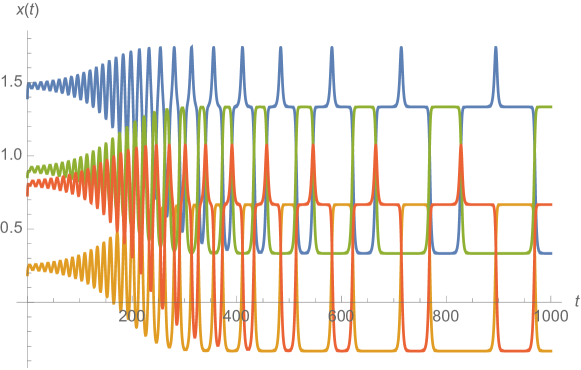
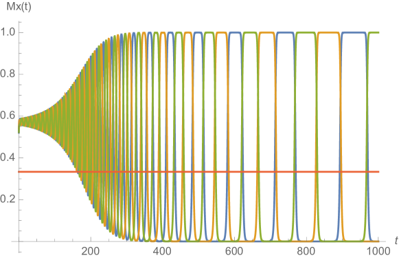
Figure 2: An evolution of the system $G(x)$. On the top we plot the exact simulation, and on the bottom we plot the solution left-multiplied by the matrix $M$.

B.2 Lorenz–Sel’kov system

Here we want to give an example of a chaotic system that lives on a simplicial complex. In particular we will choose a combination of two systems: the first will be the well-known Lorenz system [29], and the second will be the Sel’kov model for glycolysis [42] (mostly famous in the math community for being a realistic system that has a Hopf bifurcation, but in this example we choose parameters to get an attracting limit cycle).

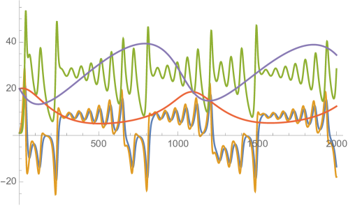
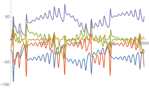
Figure 3: One example of the system (168) with $\sigma=10$, $\beta=8/3$, $\rho=28$, $a=0.1$, and $b=1.5$ .

Let us consider the simplicial complex denoted in the left of Figure 1, where we always choose orientations to point “upward” in the vertex number. In particular, this gives

$$\partial t_{1}=e_{1}+e_{2}-e_{3},\quad\partial t_{2}=e_{3}-e_{4}+e_{5}$$

and

$$\partial e_{1} =v_{2}-v_{1},\quad\partial e_{2}=v_{3}-v_{2},\quad\partial e_{3}=v_{3}-v_{1},$$

$$\partial e_{4} =v_{4}-v_{1},\quad\partial e_{5}=v_{4}-v_{3}.$$

We can compute that

$$B_{1}=\begin{pmatrix}-1&0&-1&-1&0\\ 1&-1&0&0&0\\ 0&1&1&0&-1\\ 0&0&0&1&1\end{pmatrix},\quad B_{2}=\begin{pmatrix}1&0\\ 1&0\\ -1&1\\ 0&-1\\ 0&1\end{pmatrix}$$

It is not hard to see that $B_{1}$ has rank 3 and $B_{2}$ has rank 2, so according to the terminology of Definition 3.7, this means that $r_{1}=3$, $r_{2}=2$, and $n_{1}=5$, so that any system on $C_{1}(X)$ will be a system of type $(3,2,5)$; namely a system on $\mathbb{R}^{3}$ and an independent system on $\mathbb{R}^{2}$.

Now let us recall the Lorenz system:

$$\frac{d}{dt}\begin{pmatrix}x\\ y\\ z\end{pmatrix}=\begin{pmatrix}\sigma(y-x)\\ x(\rho-z)-y\\ xy-\beta x\end{pmatrix}$$

and the Selkov model:

$$\frac{d}{dt}\begin{pmatrix}\xi\\ \eta\end{pmatrix}=\begin{pmatrix}-\xi+a\eta+\xi^{2}\eta/400\\ b-a\eta-\xi^{2}\eta/400\end{pmatrix}.$$

The standard presentation of this model is the same as above, but without dividing by the factors of 400 in the nonlinearity. We did this division so that the amplitude of the limit cycle in the Sel’kov system would be comparable to the amplitude of the Lorenz oscillator with the standard parameters. We can embed these into $\mathbb{R}^{5}$ by taking the direct sum of the dynamics:

$$\frac{d}{dt}\begin{pmatrix}x\\ y\\ z\\ \xi\\ \eta\end{pmatrix}=H(x,y,z,\xi,\eta):=\begin{pmatrix}\sigma(y-x)\\ x(\rho-z)-y\\ xy-\beta x\\ -\xi+a\eta+\xi^{2}\eta/400\\ b-a\eta-\xi^{2}\eta/400\end{pmatrix}.$$ (168)

We now want to construct the isomorphism that sends this system into a flow of the form (1). We can basically do the following: the first three rows of $B_{1}$ are linearly independent, and thus form a basis for the column space of $B_{1}^{\intercal}$, and the columns of $B_{2}$ are linearly independent. So we want $M^{-1}$ to be the $5\times 5$ matrix that sends the standard basis to these five vectors, and $M$ to be its inverse, so

$$M^{-1}=\left(\begin{array}[]{ccccc}-1&0&-1&-1&0\\ 1&-1&0&0&0\\ 0&1&1&0&-1\\ 1&1&-1&0&0\\ 0&0&1&-1&1\\ \end{array}\right),\quad M=\frac{1}{8}\left(\begin{array}[]{ccccc}-1&4&1&3&1\\ -1&-4&1&3&1\\ -2&0&2&-2&2\\ -5&-4&-3&-1&-3\\ -3&-4&-5&1&3\\ \end{array}\right)$$

From this, we can define $G(x)=M^{-1}H(Mx)$, and this is a flow on the edge space of this simplex.

We plot the results of a simulation of this system in Figure 3. We plot the dynamics of $H$ and the dynamics of $G$. In the $H$ system, the Lorenz oscillator and the limit cycle are completely disjoint, and we can see this in the timeseries. In the $G$ system (the system on the simplicial complex), these two get mixed up and we get something like a “breathing” Lorenz oscillator.

References

• [1] Manuela Aguiar, Christian Bick, and Ana Dias. Network dynamics with higher-order interactions: Coupled cell hypernetworks for identical cells and synchrony. arXiv preprint arXiv:2201.09379, 2022.
• [2] Fernando Antoneli, Ana Paula S Dias, and Rui C Paiva. Hopf bifurcation in coupled cell networks with interior symmetries. SIAM Journal on Applied Dynamical Systems, 7(1):220–248, 2008.
• [3] Albert-László Barabási et al. Network Science. Cambridge university press, 2016.
• [4] Sergio Barbarossa and Stefania Sardellitti. Topological signal processing over simplicial complexes. IEEE Transactions on Signal Processing, 2020.
• [5] Danielle Bassett and Olaf Sporns. Network neuroscience. Nature Neuroscience, 20(3):353–364, 2017.
• [6] Federico Battiston, Giulia Cencetti, Iacopo Iacopini, Vito Latora, Maxime Lucas, Alice Patania, Jean-Gabriel Young, and Giovanni Petri. Networks beyond pairwise interactions: structure and dynamics. Physics Reports, 2020.
• [7] Austin R Benson, Rediet Abebe, Michael T Schaub, Ali Jadbabaie, and Jon Kleinberg. Simplicial closure and higher-order link prediction. Proceedings of the National Academy of Sciences, 115(48):E11221–E11230, 2018.
• [8] Claude Berge. Hypergraphs: combinatorics of finite sets, volume 45. Elsevier, 1984.
• [9] Ginestra Bianconi. Higher-order networks. Elements in Structure and Dynamics of Complex Networks, 2021.
• [10] Stefano Boccaletti, Vito Latora, Yamir Moreno, Martin Chavez, and D.-U. Hwang. Complex networks: Structure and dynamics. Physics reports, 424(4-5):175–308, 2006.
• [11] Béla Bollobás. Combinatorics: set systems, hypergraphs, families of vectors, and combinatorial probability. Cambridge University Press, 1986.
• [12] Owen Courtney and Ginestra Bianconi. Generalized network structures: The configuration model and the canonical ensemble of simplicial complexes. Physical Review E, 93(6):062311, 2016.
• [13] Carina Curto. What can topology tell us about the neural code? Bulletin of the American Mathematical Society, 54(1):63–78, 2017.
• [14] Lee DeVille and Eugene Lerman. Modular dynamical systems on networks. Journal of the European Mathematical Society, 17(12):2977–3013, 2015.
• [15] Ana Paula S Dias and Jeroen SW Lamb. Local bifurcation in symmetric coupled cell networks: linear theory. Physica D: Nonlinear Phenomena, 223(1):93–108, 2006.
• [16] Chad Giusti, Robert Ghrist, and Danielle Bassett. Two’s company, three (or more) is a simplex. Journal of Computational Neuroscience, 41(1):1–14, 2016.
• [17] Martin Golubitsky and Ian Stewart. Nonlinear dynamics of networks: the groupoid formalism. Bulletin of the american mathematical society, 43(3):305–364, 2006.
• [18] Martin Golubitsky, Ian Stewart, Pietro-Luciano Buono, and JJ Collins. Symmetry in locomotor central pattern generators and animal gaits. Nature, 401(6754):693–695, 1999.
• [19] Martin Golubitsky, Ian Stewart, and Andrei Török. Patterns of synchrony in coupled cell networks with multiple arrows. SIAM Journal on Applied Dynamical Systems, 4(1):78–100, 2005.
• [20] John Guckenheimer and Philip Holmes. Structurally stable heteroclinic cycles. In Mathematical Proceedings of the Cambridge Philosophical Society, volume 103, pages 189–192. Cambridge University Press, 1988.
• [21] Allen Hatcher. Algebraic Topology. Cambridge University Press, 2002.
• [22] Roger A. Horn and Charles R. Johnson. Matrix analysis. Cambridge University Press, Cambridge, second edition, 2013.
• [23] Iacopo Iacopini, Giovanni Petri, Alain Barrat, and Vito Latora. Simplicial models of social contagion. Nature Communications, 10(1):1–9, 2019.
• [24] Lida Kanari, Pawel Dlotko, Martina Scolamiero, Ran Levi, Julian Shillcock, Kathryn Hess, and Henry Markram. A topological representation of branching neuronal morphologies. Neuroinformatics, 16(1):3–13, 2018.
• [25] Steffen Klamt, Utz-Uwe Haus, and Fabian Theis. Hypergraphs and cellular networks. PLoS Comput Biol, 5(5):e1000385, 2009.
• [26] Christophe Ladroue, Shuixia Guo, Keith Kendrick, and Jianfeng Feng. Beyond element-wise interactions: identifying complex interactions in biological processes. PloS one, 4(9):e6899, 2009.
• [27] Renaud Lambiotte, Martin Rosvall, and Ingo Scholtes. From networks to optimal higher-order models of complex systems. Nature Physics, 15(4):313–320, 2019.
• [28] Lek-Heng Lim. Hodge Laplacians on graphs. Siam Review, 62(3):685–715, 2020.
• [29] Edward N Lorenz. Deterministic nonperiodic flow. Journal of atmospheric sciences, 20(2):130–141, 1963.
• [30] Abubakr Muhammad and Magnus Egerstedt. Control using higher order Laplacians in network topologies. In Proc. of 17th International Symposium on Mathematical Theory of Networks and Systems, pages 1024–1038. Citeseer, 2006.
• [31] Daan Mulder and Ginestra Bianconi. Network geometry and complexity. Journal of Statistical Physics, 173(3-4):783–805, 2018.
• [32] James R. Munkres. Elements of Algebraic Topology. Addison-Wesley Publishing Company, Menlo Park, CA, 1984.
• [33] Mark Newman. Networks. Oxford University Press, 2018.
• [34] Mark Newman, Albert-László Barabási, and Duncan J Watts. The structure and dynamics of networks. Princeton University Press, 2006.
• [35] Eddie Nijholt, Bob Rink, and Jan Sanders. Graph fibrations and symmetries of network dynamics. Journal of Differential Equations, 261(9):4861–4896, 2016.
• [36] Eddie Nijholt, Bob Rink, and Jan Sanders. Center manifolds of coupled cell networks. SIAM Review, 61(1):121–155, 2019.
• [37] Eddie Nijholt, Bob W Rink, and Sören Schwenker. Quiver representations and dimension reduction in dynamical systems. SIAM Journal on Applied Dynamical Systems, 19(4):2428–2468, 2020.
• [38] Alice Patania, Giovanni Petri, and Francesco Vaccarino. The shape of collaborations. EPJ Data Science, 6(1):18, 2017.
• [39] Mason A Porter. Nonlinearity + networks: A 2020 vision. In Emerging Frontiers in Nonlinear Science, pages 131–159. Springer, 2020.
• [40] Theodore Roman, Amir Nayyeri, Brittany Terese Fasy, and Russell Schwartz. A simplicial complex-based approach to unmixing tumor progression data. BMC bioinformatics, 16(1):254, 2015.
• [41] Vsevolod Salnikov, Daniele Cassese, and Renaud Lambiotte. Simplicial complexes and complex systems. European Journal of Physics, 40(1):014001, 2018.
• [42] EE Sel’Kov. Self-oscillations in glycolysis 1. a simple kinetic model. European Journal of Biochemistry, 4(1):79–86, 1968.
• [43] Daniel Hernández Serrano, Juan Hernández-Serrano, and Darío Sánchez Gómez. Simplicial degree in complex networks. applications of topological data analysis to network science. Chaos, Solitons & Fractals, 137:109839, 2020.
• [44] Ann E Sizemore, Chad Giusti, Ari Kahn, Jean M Vettel, Richard F Betzel, and Danielle S Bassett. Cliques and cavities in the human connectome. Journal of computational neuroscience, 44(1):115–145, 2018.
• [45] Ian Stewart, Martin Golubitsky, and Marcus Pivato. Symmetry groupoids and patterns of synchrony in coupled cell networks. SIAM Journal on Applied Dynamical Systems, 2(4):609–646, 2003.
• [46] Bernadette J. Stolz, Heather A. Harrington, and Mason A. Porter. Persistent homology of time-dependent functional networks constructed from coupled time series. Chaos: An Interdisciplinary Journal of Nonlinear Science, 27(4):047410, 2017.
• [47] Leo Torres, Ann Blevins, Danielle Bassett, and Tina Eliassi-Rad. The why, how, and when of representations for complex systems. arXiv preprint arXiv:2006.02870, 2020.