itdr: An R package of Integral Transformation Methods to Estimate the SDR Subspaces in Regression

Abstract

Sufficient dimension reduction (SDR) is an effective tool for regression models, offering a viable approach to address and analyze the nonlinear nature of regression problems. This paper introduces the itdr R package, a comprehensive and user-friendly tool that introduces several functions based on integral transformation methods for estimating SDR subspaces. In particular, the itdr package incorporates two key methods, namely the Fourier method (FM) and the convolution method (CM). These methods allow for estimating the SDR subspaces, namely the central mean subspace (CMS) and the central subspace (CS), in cases where the response is univariate. Furthermore, the itdr package facilitates the recovery of the CMS through the iterative Hessian transformation (IHT) method for univariate responses. Additionally, it enables the recovery of the CS by employing various Fourier transformation strategies, such as the inverse dimension reduction method, the minimum discrepancy approach using Fourier transformation, and the Fourier transform sparse inverse regression approach, specifically designed for cases with multivariate responses. To demonstrate its capabilities, the itdr package is applied to five different datasets. Furthermore, this package is the pioneering implementation of integral transformation methods for estimating SDR subspaces, thus promising significant advancements in SDR research.

Introduction: Sufficient Dimension Reduction in Regression

Let $Y$ be a univariate response, and let $\mathbf{X}$ be a $p$-dimensional vector consisting of continuous predictors, denoted as $\mathbf{X}=({X}_{1},\cdots,{X}_{p})^{T}$. The conditional distribution of $Y$ given $\mathbf{X}$ is denoted as $F_{Y|\mathbf{X}}$, and $E[Y|\mathbf{X}]$ represents the mean response at $\mathbf{X}$. When $F_{Y|\mathbf{X}}$ or $E[Y|\mathbf{X}]$ lacks a specific parametric form, nonparametric methods should be employed. However, classical methods, such as polynomial smoothing methods, become impractical as the dimension of $\mathbf{X}$ increases. To address the curse of dimensionality, several dimension reduction methods have been proposed. Sufficient dimension reduction (SDR) stands out as one of the most important and successful approaches that have garnered considerable interest in recent years. The SDR method seeks to project $\mathbf{X}$ onto a lower-dimensional subspace in a manner that enables the formation of the regression of $Y$ on $\mathbf{X}$ without loss of information about $F_{Y|\mathbf{X}}$ or $E[Y|\mathbf{X}]$, thus mitigating the curse of dimensionality.

The SDR theory has its origins in the seminal work of Li (1991) and Cook and Weisberg (1991). The primary objective of SDR is to estimate a $p\times d$ matrix $\boldsymbol{\Gamma}$, $d\leq p$, with the aim of replacing the $p$-dimensional predictor vector X with a $d$-dimensional vector $\boldsymbol{\Gamma}^{T}\textbf{X}$. This substitution strives to preserve all relevant information about the responses $Y$ without any loss. Importantly, the SDR technique does not impose any specific model assumptions, as discussed by Cook (1998). In a more general context, we consider the following regression model

$$Y=g(\boldsymbol{\Gamma}^{T}\textbf{X})+\varepsilon,$$ (1)

where $g(\cdot)$ is an unknown smooth link function and $\varepsilon$ denotes the error term. Within this framework, we can define the following SDR subspaces.

Definition 1

Suppose $\mathcal{S}\subseteq\mathbb{R}^{p}$ with projection $\mathcal{P_{S}}$, and let $\mathcal{P_{S}}:\mathbb{R}^{p}\to\mathcal{S}$ be the orthogonal projection operator onto a $d~{}(<p)$-dimensional subspace $\mathcal{S}$. The subspace $\mathcal{S}$ is a sufficient dimension reduction subspace if

$$Y\mathchoice{\mathrel{\hbox to0.0pt{$\displaystyle\perp$\hss}\mkern 2.0mu{\displaystyle\perp}}}{\mathrel{\hbox to0.0pt{$\textstyle\perp$\hss}\mkern 2.0mu{\textstyle\perp}}}{\mathrel{\hbox to0.0pt{$\scriptstyle\perp$\hss}\mkern 2.0mu{\scriptstyle\perp}}}{\mathrel{\hbox to0.0pt{$\scriptscriptstyle\perp$\hss}\mkern 2.0mu{\scriptscriptstyle\perp}}}\textbf{X}|\mathcal{P_{S}}\textbf{X},$$ (2)

where $\mathchoice{\mathrel{\hbox to0.0pt{$\displaystyle\perp$\hss}\mkern 2.0mu{\displaystyle\perp}}}{\mathrel{\hbox to0.0pt{$\textstyle\perp$\hss}\mkern 2.0mu{\textstyle\perp}}}{\mathrel{\hbox to0.0pt{$\scriptstyle\perp$\hss}\mkern 2.0mu{\scriptstyle\perp}}}{\mathrel{\hbox to0.0pt{$\scriptscriptstyle\perp$\hss}\mkern 2.0mu{\scriptscriptstyle\perp}}}$ indicates independence. The intersection of all dimension reduction subspaces that satisfies Equation (2) is called the central dimension reduction subspace, or “Central Subspace (CS)”. It is denoted as $\mathcal{S}_{Y|\textbf{X}}$.

The dimension of $\mathcal{S}_{Y|\textbf{X}}$, denoted as $d=dim(\mathcal{S}_{Y|\textbf{X}})$ is referred to as the structural dimension of the regression $Y$ on $\mathbf{X}$. Cook (1998) demonstrated the existence and uniqueness of $\mathcal{S}_{Y|\textbf{X}}$ under certain mild conditions. Similarly, Definition 1 can be extended to include cases where the conditional mean function $E[Y|\textbf{X}]$ is of interest. This extension leads to the concept of central mean subspace, introduced by Cook and Li (2002).

Definition 2

Suppose an orthogonal projection $\mathcal{P_{S}}:\mathbb{R}^{p}\to\mathcal{S}$ denote the projection operator onto a $d~{}(<p)$-dimensional subspace $\mathcal{S}$. Then, $\mathcal{S}$ is a mean dimension reduction subspace for conditional mean if

$$Y\mathchoice{\mathrel{\hbox to0.0pt{$\displaystyle\perp$\hss}\mkern 2.0mu{\displaystyle\perp}}}{\mathrel{\hbox to0.0pt{$\textstyle\perp$\hss}\mkern 2.0mu{\textstyle\perp}}}{\mathrel{\hbox to0.0pt{$\scriptstyle\perp$\hss}\mkern 2.0mu{\scriptstyle\perp}}}{\mathrel{\hbox to0.0pt{$\scriptscriptstyle\perp$\hss}\mkern 2.0mu{\scriptscriptstyle\perp}}}E[Y|\textbf{X}]|\mathcal{P_{S}}\textbf{X}.$$ (3)

The intersection of all mean dimension reduction subspaces that satisfies the condition given in Equation (3) is called the mean dimension reduction subspace, or “Central Mean Subspace (CMS)”. It is denoted by $\mathcal{S}_{E[Y|\textbf{X}]}$.

Several parametric and nonparametric estimation methods have been developed to estimate the CS and CMS. These include sliced inverse regression (SIR; Li, 1991), sliced average variance estimation (SAVE; Cook and Weisberg, 1991), inverse regression estimation method (IRE; Cook and Ni, 2005), and Fourier transformation method for inverse dimension reduction (Weng and Yin, 2018, 2022; Weng, 2022), among others. Nonlinear dimension reduction techniques, such as kernel PCA (KPCA), generalized SIR (GSIR), and generalized SAVE (GSAVE) methods, have been proposed to estimate the nonlinear central subspace in order to overcome the limitations of linear combinations of covariates in principal component analysis (PCA), SIR, and SAVE methods (see Li, 2018). Moreover, Ma and Zhu (2013) and Feng et al. (2013) proposed the efficient estimator (Eff) and partial SAVE (pSAVE) methods, respectively, for estimating the CS. Likelihood-based SDR methods, such as covariance reduction (CORE; Cook and Forzani, 2008a), likelihood acquired directions (LAD; Cook and Forzani, 2009), and principal fitted components (PFC; Cook, 2007; Cook and Forzani, 2008b) have been proposed for the CS estimation. Various approaches have been proposed to estimate CMS, such as the principal Hessian direction (PHD; Li, 1992), iterative Hessian transformation (IHT; Cook and Li, 2002), and the structure adaptive method (SAM; Hristache et al., 2001). The minimum average estimation (MAVE; Xia et al., 2002) and outer product gradient (OPG; Xia et al., 2002) methods are implemented for estimating both the CS and the CMS. Furthermore, the Fourier transformation method (FM; Zhu and Zeng, 2006) and the convolution transformation method (CM; Zeng and Zhu, 2010) have been employed to estimate both the CS and the CMS.

The R package ldr, developed by Adragni and Raim (2014), implements three likelihood-based SDR methods, i.e., CORE, LAD, and PFC for estimating the CS. The R package $\mathbf{dr}$, developed by Weisberg (2015), implements several SDR approaches, including the SIR, SAVE, and IRE methods to estimate the CS. It also encompasses the PHD method to estimate the CMS and provides several helper functions to estimate additional model parameters in each case. The MAVE R package, developed by Hang and Xia (2019), implements the MAVE and OPG methods to estimate the CS and CMS. The R package orthoDr, developed by Zhu et al. (2019), provides estimates of the CS using the Eff and pSAVE methods. Finally, the nsdr R package, developed by Li and Kim (2021), implements the KPCA, GSIR, and GSAVE methods to estimate the CS.

Our R package, itdr, performs the latest developments in the estimation of the CS and CMS using integral transformation methods. The itdr provides functions to estimate both the CS and CMS using various approaches. These include the FM approach proposed by Zhu and Zeng (2006) under the normality assumption of the predictors, the CM approach introduced by Zeng and Zhu (2010), and the IHT method by Cook and Li (2002). Furthermore, Zeng and Zhu (2010) established a general framework for any integral transformation method that can be used to estimate the CS and CMS when the predictor vector follows either a multivariate normal distribution, an elliptically contoured distribution, or without imposing any distributional assumption on it. In this framework, a kernel smoother is applied to approximate the unknown distribution function of the predictor variables. Our itdr package also includes some helper functions to estimate the dimension of SDR subspaces and the tuning parameters of the FM and CM algorithms. The itdr package facilitates the estimation of the CS using the inverse regression approach via Fourier transformation (invFM) proposed by Weng and Yin (2018), the minimum discrepancy approach(Weng and Yin, 2022), and the sparse Fourier transform inverse regression method (Weng, 2022). These Fourier transformation methods allow for using either univariate or multivariate responses and provide an estimate for the CS. The R package itdr has been uploaded to CRAN and is available at https://CRAN.R-project.org/package=itdr.

The remainder of this paper is organized as follows; we start with a brief overview of six integral transformation methods employed for estimating the SDR subspaces. Once the methods are introduced, the subsequent sections are devoted to demonstrating the utilization of functions within the itdr package. Specifically, we illustrate how to estimate the tuning parameters, select the dimension of SDR subspaces, and obtain accurate estimations of the SDR subspaces using various datasets available within the itdr package.

Integral Transformation Methods (ITMs) and Candidate Matrices

In this section, we provide a summary of the theoretical framework of integral transformation methods proposed by Zhu and Zeng (2006) and Zeng and Zhu (2010). These methods are utilized to drive estimators for the SDR subspaces. All of these methods employ the spectral-decomposition-based procedure. The first step of each method involves constructing a nonnegative definite symmetric matrix, denoted as $\mathbf{M}\in\mathbb{R}^{p\times p}$, referred to as a candidate matrix. The second step consists of performing the spectral-decomposition of a sample version of $\mathbf{M}$, denoted as $\widehat{\mathbf{M}}$. Then, an orthogonal basis is formed by the first $d$ eigenvectors corresponding to the leading $d$ eigenvalues of $\widehat{\mathbf{M}}$, which serves as an estimation of the target SDR subspace. The candidate matrices based on the integral transformation method, whose column spaces are identical to the CMS and CS, are respectively denoted as $\mathbf{M}_{ITM}$, and $\mathbf{M}_{ITC}$.

First, we consider the derivation of the candidate matrix $\mathbf{M}_{ITM}$ for estimating the CMS in regression. Suppose $m(\mathbf{x})=E(Y|\mathbf{X}=\mathbf{x})$; then from the model given in Equation (1), we can express $m(\mathbf{x})$ as $m(\mathbf{x})=g(\boldsymbol{\Gamma}^{T}\mathbf{x})$. By applying the chain rule of differentiation, we establish the following relationship between the gradient operator of $m(\mathbf{x})$ and the link function $g(\mathbf{u})$, where $\mathbf{u}=\boldsymbol{\Gamma}^{T}\mathbf{x}$,

$$\frac{\partial}{\partial\mathbf{x}}m(\mathbf{x})=\boldsymbol{\Gamma}\frac{\partial}{\partial\mathbf{u}}g(\mathbf{u}).$$ (4)

Since $\boldsymbol{\Gamma}\frac{\partial}{\partial\mathbf{u}}g(\mathbf{u})\in\mathcal{S}_{E[Y|\mathbf{X}]}$, it follows that $\frac{\partial}{\partial\mathbf{x}}m(\mathbf{x})\in\mathcal{S}_{E[Y|\mathbf{X}]}$. This further implies that $E\left[\frac{\partial}{\partial\mathbf{X}}m(\mathbf{X})\right]\in\mathcal{S}_{E[Y|\mathbf{X}]}$ providing the average derivative estimate (ADE). However, the ADE method can only generate one direction, limiting its ability to estimate the CMS of dimensions higher than one. Additionally, the ADE method fails when $E\left[\frac{\partial}{\partial\mathbf{X}}m(\mathbf{X})\right]=0$. More detailed discussions can be found in Zeng and Zhu (2010). These disadvantages can be overcome by introducing an appropriate family of weight functions $\{W(\mathbf{x},\mathbf{u}):\mathbf{u}\in\mathbb{R}^{p}\}$, such that $E\left[W(\mathbf{x},\mathbf{u})\frac{\partial}{\partial\mathbf{X}}m(\mathbf{X})\right]\neq 0$, where $\mathbf{u}\in\mathbb{R}^{p}$ represents the family index. Note that a single weight function is sufficient to overcome the first drawback; however, different weight functions produce different vectors in the CMS, enabling the estimation of the entire CMS. The weighted ADE is then defined as

$$\boldsymbol{\psi}(\mathbf{u})=E\left[\frac{\partial}{\partial\mathbf{X}}m(\mathbf{X})W(\mathbf{X},\mathbf{u})\right]=\int\frac{\partial}{\partial\mathbf{x}}m(\mathbf{x})W(\mathbf{x},\mathbf{u})f(\mathbf{x})d\mathbf{x}.$$ (5)

Indeed, $\boldsymbol{\psi}(\mathbf{u})$ represents the integral transformation of the density weighted gradient of $m(\mathbf{x})$, and $W(\mathbf{x},\mathbf{u})$ is the nondegenerate kernel function associated with this transformation. The most commonly chosen weight function are $W_{1}(\mathbf{x},\mathbf{u})=\exp\{i\mathbf{u}^{T}\mathbf{x}\}$ and $W_{2}(\mathbf{x},\mathbf{u})=H(\mathbf{u}-\mathbf{x})$, where $H(\cdot)$ is an absolutely integrable function. The integral transformation using the weigh function $W_{1}(\mathbf{x},\mathbf{u})$ is referred to as the Fourier transformation method (FM), while the transformation using the weight function $W_{2}(\mathbf{x},\mathbf{u})$ is known as the convolution transformation method (CM). By applying the integration by parts to Equation (5), we obtain

$$\boldsymbol{\psi}(\mathbf{u})=-E\left[Y\phi(\mathbf{X},\mathbf{u})\right],$$ (6)

where $\phi(\mathbf{x},\mathbf{u})=\frac{\partial}{\partial\mathbf{x}}W(\mathbf{x},\mathbf{u})+W(\mathbf{x},\mathbf{u})\mathbf{g}(\mathbf{x})$ and $\mathbf{g}(\mathbf{x})=\frac{\partial}{\partial\mathbf{x}}\log f(\mathbf{x})$. Note that the expression $\boldsymbol{\psi}(\mathbf{u})$ in Equation (5) depends on the mean function $m(\mathbf{x})$, while $\boldsymbol{\psi}(\mathbf{u})$ in Equation (6) does not rely on $m(\mathbf{x})$. This implies that we can calculate $\boldsymbol{\psi}(\mathbf{u})$ without the need to fit or estimate the link function $g(\cdot)$ or its derivatives. Therefore, $\boldsymbol{\psi}(\mathbf{u})$ in Equation (6) is used to define a candidate matrix for $\mathcal{S}_{E[{Y|\mathbf{X}}]}$. This candidate matrix, whose column space is equal to the CMS, is denoted by $\mathbf{M}_{ITM}$ and defined as follows

$$\mathbf{M}_{ITM}=\int\boldsymbol{\psi}(\mathbf{u})\overline{\boldsymbol{\psi}}^{T}(\mathbf{u})K(\mathbf{u})d\mathbf{u}=E[\mathcal{\mathbf{U}}_{ITM}(\mathbf{Z}_{1},\mathbf{Z}_{2})],$$ (7)

where $\overline{\boldsymbol{\psi}}(\cdot)$ denotes the conjugation of $\boldsymbol{\psi}(\cdot)$, $\mathbf{z}=(y,\mathbf{x})$, $\mathbf{Z}_{1}$ and $\mathbf{Z}_{2}$ are two independent realizations of $\mathbf{Z}$, and

$$\mathcal{\mathbf{U}}_{ITM}(\mathbf{z}_{1},\mathbf{z}_{2})=y_{1}y_{2}\int\phi(\mathbf{x}_{1},\mathbf{u})\phi^{T}(\mathbf{x}_{2},\mathbf{u})K(\mathbf{u})d\mathbf{u}.$$ (8)

Note that for the FM method, $K(\mathbf{u})$ is set as $K(\mathbf{u})=(2\pi\sigma_{u}^{2})^{-p/2}\exp\{-||\mathbf{u}||/2\sigma_{u}^{2}\}$, and for the CM it is set to $K(\mathbf{u})=1$. Let $\mathcal{S}(\mathbf{M}_{ITM})$ denote the subspace spanned by the columns of $\mathbf{M}_{ITM}$. Then, Lemma 1 establishes that the column space of $\mathbf{M}_{ITM}$ is the same as the CMS.

Lemma 1

The result stated in Equation (6) holds under the following conditions:

• The function $f(\mathbf{x})\frac{\partial}{\partial\mathbf{x}}m(\mathbf{x})$ exists and is absolutely integrable.

• The expression $W(\mathbf{x},\mathbf{u})m(\mathbf{x})f(\mathbf{x})$ goes to zero as $||\mathbf{x}||\to\infty$.

• The function $\log f(\mathbf{x})$ is differentiable.

Moreover, if $W(\cdot,\cdot)$ is a nondegenerate kernel for $f(\mathbf{x})\frac{\partial}{\partial\mathbf{x}}$ and $\boldsymbol{\psi}(\mathbf{u})$ is square integrate, then $\mathbf{M}_{ITM}$ is a nonnegative definite matrix and $\mathcal{S}(\mathbf{M}_{ITM})=\mathcal{S}_{E[Y|\mathbf{X}]}$.

The proof of Lemma 1 is similar to that of Proposition 2 in Zhu and Zeng (2006) and Lemma 3 in Zeng and Zhu (2010), and hence is omitted. Furthermore, a candidate matrix for the CS can be obtained by following the procedures outlined below. To derive it, it is important to note that the central mean subspace is always a subspace of the central subspace, represented as $\mathcal{S}_{E[Y|\mathbf{X}]}\subseteq\mathcal{S}_{Y|\mathbf{X}}$ Cook (1998). Let $T(Y)$ denote an arbitrary transformation of the response variable $Y$, resulting in a new response. Furthermore, let $\mathcal{S}_{E[T(Y)|\mathbf{X}]}$ denotes the CMS of $T(Y)$ on $\mathbf{X}$. It is then evident that $\mathcal{S}_{E[T(Y)|\mathbf{X}]}\subseteq\mathcal{S}_{Y|\mathbf{X}}$, but it may not be identical to $\mathcal{S}_{E[Y|\mathbf{X}]}$ Zhu and Zeng (2006). Despite the fact that two CMS $\mathcal{S}_{E[T_{1}(Y)|\mathbf{X}]}$ and $\mathcal{S}_{E[T_{2}(Y)|\mathbf{X}]}$ differ for two distinct transformations $T_{1}(\cdot)$ and $T_{2}(\cdot)$, they might cover different parts of the entire CS. Thus, by considering a collection of CMS obtained from different transformations, it becomes possible to cover the entire CS Zhu and Zeng (2006). In other words, we have

$$\mathcal{S}_{Y|\mathbf{X}}=\sum_{all~{}~{}possible~{}~{}T}\mathcal{S}_{E[T(Y)|\mathbf{X}]}.$$

Let $T_{v}(Y)$ represent a simple family of transformations, denoted as $\{T_{v}(\cdot):T_{v}(y)=\tau(y,v),\text{ for }y,v\in\mathbb{R}\}$, where $\tau(\cdot,\cdot)$ is a known function. For a given $v\in\mathbb{R}$, the conditional mean response of $T_{v}(Y)$ given $\mathbf{x}$ is defined as $m(\mathbf{x},v)=E[\tau(Y,v)|\mathbf{X}=\mathbf{x}]$. Now, let us define the integral transformation of the partial derivative of $m(\mathbf{x},v)$ with respect to $\mathbf{x}$, weighted by $W(\mathbf{x},\mathbf{u})$ as $\boldsymbol{\psi}(\mathbf{u},v)$. In other words

$$\boldsymbol{\psi}(\mathbf{u},v)=E\left[\frac{\partial m(\mathbf{X},v)}{\partial\mathbf{x}}W(\mathbf{x},\mathbf{u})\right]=-E\left[\tau(Y,v)\phi(\mathbf{X},\mathbf{u})\right].$$ (9)

Furthermore, a candidate matrix for $\mathcal{S}_{Y|\mathbf{X}}$, denoted as $\mathbf{M}_{ITC}$, is defined as

$$\mathbf{M}_{ITC}=\int\boldsymbol{\psi}(\mathbf{u},v)\boldsymbol{\psi}^{T}(\mathbf{u},v)K(\mathbf{u})d\mathbf{u}=E[\mathbf{U}_{ITC}(\mathbf{Z}_{1},\mathbf{Z}_{2})],$$ (10)

where $K(\mathbf{u})=(2\pi\sigma_{u}^{2})^{-p/2}\exp\{-||\mathbf{u}||/(2\sigma_{u}^{2})\}$ for the FM procedure and $K(\mathbf{u})=1$ for the CM procedure. In Equation (10), $\mathbf{z}=(y,\mathbf{x})$, $\mathbf{Z}_{1}$ and $\mathbf{Z}_{2}$ represent independent realizations of $\mathbf{Z}$, and

$$\mathbf{U}_{ITC}(\mathbf{z}_{1},\mathbf{z}_{2})=\int\tau(y_{1},v)\tau(y_{2},v)dv\int\phi(\mathbf{x}_{1},\mathbf{u})\phi^{T}(\mathbf{x}_{2},\mathbf{u})K(\mathbf{u})d\mathbf{u},$$ (11)

where $\tau(y,v)=(2\pi\sigma_{v}^{2})^{-1/2}\exp\{-(y-v)^{2}/(2\sigma_{v}^{2})\}$. Lemma 2 demonstrates that under certain mild conditions $\mathcal{S}_{Y|\mathbf{X}}=\sum_{v\in\mathbb{R}}\mathcal{S}_{E[T_{v}(Y)|\mathbf{X}]}$, and the column space of $\mathbf{M}_{ITC}$ in Equation (10) is the same as the central mean subspace $\mathcal{S}_{Y|\mathbf{X}}$.

Lemma 2

The results presented in Equation (9) are valid under the folloing conditions:

• $f(\mathbf{x})\frac{\partial}{\partial\mathbf{x}}m(\mathbf{x},v)$ exists and is absolutely integrable.

• $W(\mathbf{x},\mathbf{u})m(\mathbf{x},v)f(\mathbf{x})$ goes to zeros as $||\mathbf{x}||\to\infty$ .

• $\log f(\mathbf{x})$ is differentiable.

Furthermore, if $\tau(y,v)W(\mathbf{x},\mathbf{u})$ serves as nondegenerate kernal for $f(\mathbf{x})\frac{\partial}{\partial\mathbf{x}}$ and $\boldsymbol{\psi}(\mathbf{u},v)$ is square integrable, then $\mathbf{M}_{ITC}$ is a nonnegative definite matrix and $\mathcal{S}(\mathbf{M}_{ITC})=\mathcal{S}_{Y|\mathbf{X}}$.

The proof of Lemma 2 follows a similar approach to that of Proposition 6 in Zhu and Zeng (2006) and Lemma 4 in Zeng and Zhu (2010), and is therefore omitted here.

Estimation of Candidate Matrices

In this section, we discuss the estimates of the candidate matrices $\mathbf{M}_{ITM}$ and $\mathbf{M}_{ITC}$. We begin by expressing the sample versions of the candidate matrices used to estimate the CMS and the CS under the Fourier transformation method. We denote these candidate matrices as $\mathbf{M}_{FMM}$ and $\mathbf{M}_{FMC}$, respectively. First, we set $W(\mathbf{x},\mathbf{u})=\exp\{i\mathbf{u}^{T}\mathbf{x}\}$ in Equation (5). Then, the sample version of the candidate matrix under the Fourier transformation method, which targets the CMS, can be expressed as

$$\widehat{\mathbf{M}}_{FMM}^{\star}=\frac{1}{N^{2}}\sum_{i=1}^{N}\sum_{j=1}^{N}\widehat{\mathbf{U}}_{FMM}(\mathbf{Z}_{i},\mathbf{Z}_{j}),$$ (12)

where

$$\widehat{\mathbf{U}}_{FMM}(\mathbf{Z}_{1},\mathbf{Z}_{2})=y_{1}y_{2}\exp\left\{\frac{-\sigma_{u}^{2}}{2}||\mathbf{u}_{12}||^{2}\right\}\left[\sigma_{u}^{2}\mathbf{I}_{p}+[{\mathbf{g}}(\mathbf{x}_{1})-\sigma_{u}^{2}\mathbf{u}_{12}][{\mathbf{g}}(\mathbf{x}_{2})+\sigma_{u}^{2}\mathbf{u}_{12}]^{T}\right].$$ (13)

Here ${\mathbf{g}}(\mathbf{x})=\frac{\frac{\partial}{\partial\mathbf{x}}{f}(\mathbf{x})}{{f}(\mathbf{x})}$, and $\mathbf{u}_{12}=\mathbf{x}_{1}-\mathbf{x}_{2}$. Note that the density function ${f}(\mathbf{x})$ appears in the denominator of ${\mathbf{g}}(\mathbf{x})$. Therefore, to mitigate the negative effect of small values of ${f}(\mathbf{x})$ on the estimation, the estimator $\widehat{\mathbf{M}}_{FMM}^{\star}$ given in Equation (12) is modified as follows

$$\widehat{\mathbf{M}}_{FMM}=\frac{1}{N^{2}}\sum_{i=1}^{N}\sum_{j=1}^{N}\widehat{\mathbf{U}}_{FMM}(\mathbf{Z}_{i},\mathbf{Z}_{j})\widehat{I}_{i}\widehat{I}_{j},$$ (14)

where $\widehat{\mathbf{U}}_{FMM}$ is the same as in Equation (13). Additionally, for a predetermined threshold value $b$, we defined $\widehat{I}_{(\cdot)}=1$ if ${f}(\mathbf{x}_{(\cdot)})>b$ and $\widehat{I}_{(\cdot)}=0$ otherwise. Similarly, by setting $\tau(y,v)=(2\pi\sigma_{v}^{2})^{-1/2}\exp\{-(y-v)^{2}/(2\sigma_{v}^{2})\}$, the sample version of the candidate matrix $\mathbf{M}_{FMC}$ targeting the CS is given as

$$\widehat{\mathbf{M}}_{FMC}=\frac{1}{N^{2}}\sum_{i=1}^{N}\sum_{j=1}^{N}\widehat{\mathbf{U}}_{FMC}(\mathbf{Z}_{i},\mathbf{Z}_{j})\widehat{I}_{i}\widehat{I}_{j},$$ (15)

where

$$\widehat{\mathbf{U}}_{FMC}(\mathbf{Z}_{1},\mathbf{Z}_{2})=\exp\left\{\frac{-\sigma_{u}^{2}}{2}||\mathbf{u}_{12}||^{2}-\frac{\sigma_{v}^{2}}{2}v^{2}_{12}\right\}\left[\sigma_{u}^{2}\mathbf{I}_{p}+[\mathbf{g}(\mathbf{x}_{1})-\sigma_{u}^{2}\mathbf{u}_{12}][\mathbf{g}(\mathbf{x}_{2})+\sigma_{u}^{2}\mathbf{u}_{12}]^{T}\right],$$ (16)

where $\mathbf{u}_{12}=\mathbf{x}_{1}-\mathbf{x}_{2}$, and $v_{12}=y_{1}-y_{2}$.

Now, we express the sample versions of the candidate matrices for estimating the CMS and CS under the convolution transformation method (CM). These candidate matrices are denoted as $\mathbf{M}_{CMM}$ and $\mathbf{M}_{CMC}$, respectively. Their column spaces are identical to the CMS and the CS. For both the CMS and CS, we set the same weight function $W(\mathbf{x},\mathbf{u})=H(\mathbf{x}-\mathbf{u})$ in Equation (5), where $H(\mathbf{x}-\mathbf{u})=(2\pi\sigma_{u}^{2})^{-p/2}\exp\{(\mathbf{x}-\mathbf{u})^{T}(\mathbf{x}-\mathbf{u})/(2\sigma_{u}^{2})\}$. By applying simple algebra manipulations, we obtain

$$\widehat{\mathbf{M}}_{CMM}=\frac{1}{N^{2}}\sum_{i=1}^{N}\sum_{j=1}^{N}\widehat{\mathbf{U}}_{CMM}(\mathbf{Z}_{i},\mathbf{Z}_{j})\widehat{I}_{i}\widehat{I}_{j},$$ (17)

where

$$\widehat{\mathbf{U}}_{CMM}(\mathbf{Z}_{1},\mathbf{Z}_{2})=y_{1}y_{2}\exp\left\{\frac{-||\mathbf{u}_{12}||^{2}}{4\sigma_{u}^{2}}\right\}\left[\frac{1}{2\sigma_{u}^{2}}\mathbf{I}_{p}+[\mathbf{g}(\mathbf{x}_{1})-\frac{1}{2\sigma_{u}^{2}}\mathbf{u}_{12}][\mathbf{g}(\mathbf{x}_{2})+\frac{1}{2\sigma_{u}^{2}}\mathbf{u}_{12}]^{T}\right].$$ (18)

Similarly, we choose $\tau(y,v)=\exp\{-(y-v)^{2}/(2\sigma_{v}^{2})\}$ to derive an expression for the candidate matrix $\mathbf{M}_{CMC}$ that targets the CS. The sample version of $\mathbf{M}_{CMC}$ is given by

$$\widehat{\mathbf{M}}_{CMC}=\frac{1}{N^{2}}\sum_{i=1}^{N}\sum_{j=1}^{N}\widehat{\mathbf{U}}_{CMC}(\mathbf{Z}_{i},\mathbf{Z}_{j})\widehat{I}_{i}\widehat{I}_{j},$$ (19)

where

$$\widehat{\mathbf{U}}_{CMC}(\mathbf{Z}_{1},\mathbf{Z}_{2})=\exp\left\{-\frac{v_{12}^{2}}{4\sigma_{v}^{2}}-\frac{||\mathbf{u}_{12}||^{2}}{4\sigma_{u}^{2}}\right\}\left[\frac{1}{2\sigma_{u}^{2}}\mathbf{I}_{p}+[\mathbf{g}(\mathbf{x}_{1})-\frac{1}{2\sigma_{u}^{2}}\mathbf{u}_{12}][\mathbf{g}(\mathbf{x}_{2})+\frac{1}{2\sigma_{u}^{2}}\mathbf{u}_{12}]^{T}\right].$$ (20)

Estimating Density Functions

The density function $f(\mathbf{x})$ which appears in the term $\mathbf{g}(\mathbf{x})=\frac{\frac{\partial}{\partial\mathbf{x}}f(\mathbf{x})}{f(\mathbf{x})}$ is unknown. In this section, we discuss the methods that are used to approximate the unknown density function $f(\mathbf{x})$ at a given point $\mathbf{x}$. One approach is to assume $f(\mathbf{x})=f_{0}(\mathbf{x};\boldsymbol{\theta})$, where $f_{0}$ is a known function and $\boldsymbol{\theta}$ is a vector of unknown parameters. By making this assumption, we can estimate $f(\mathbf{x})$ and $g(\mathbf{x})$ parametrically. A well-known parametric density is the Gaussian density function, which can be considered for $f(\mathbf{x})$. Under the normality assumption, it can be shown that $g(\mathbf{x})=-\mathbf{x}$.

Alternatively, we can employ a nonparametric method to estimate $f(\mathbf{x})$ without imposing distributional assumptions on $\mathbf{X}$. In this setting, Zeng and Zhu (2010) utilized kernel density estimation approach to estimate $f(\mathbf{x})$. They proposed the following estimator for $\mathbf{g}(\mathbf{x})$ at a specific point $\mathbf{x}_{0}$

$$\widehat{\mathbf{g}}(\mathbf{x}_{0})=\frac{\frac{\partial}{\partial\mathbf{x}_{0}}\widehat{f}(\mathbf{x}_{0})}{\widehat{f}(\mathbf{x}_{0})}=\frac{(nh^{p+1})^{-1}\sum_{\ell=1}^{n}K^{{}^{\prime}}((\mathbf{x}_{0}-\mathbf{x}_{\ell})/h)}{(nh^{p})^{-1}\sum_{\ell=1}^{n}K((\mathbf{x}_{0}-\mathbf{x}_{\ell})/h)},$$ (21)

where $\widehat{f}(\mathbf{x}_{0})=(nh^{p})^{-1}\sum_{\ell=1}^{n}K((\mathbf{x}_{0}-\mathbf{x}_{\ell})/h)$, $K(\cdot)$ is a kernel function with bandwidth $h$, and $K^{{}^{\prime}}(\cdot)$ represents the derivative of $K(\cdot)$.

Moreover, another option is to assume an elliptically contoured distribution for $f(\mathbf{x})$. It has been shown that, under an elliptically contoured distribution, an estimate for $g(\mathbf{x})$ can be obtained as follows (for more details, see Zeng and Zhu, 2010)

$$\widetilde{\mathbf{g}}(\mathbf{x}_{i})=\frac{\mathbf{x}_{i}}{r_{i}}\frac{\widetilde{f}^{\prime}(r_{i})}{\widetilde{f}(r_{i})}-\frac{p-1}{r_{i}^{2}}\mathbf{x}_{i},$$ (22)

where $r_{i}=||\mathbf{x}_{i}||$, and $\{r_{i}\}_{i=1}^{n}$ represents an independent and identically distributed (iid) sample from $f(r)$. Additionally, $\widetilde{f}(\cdot)$ denotes the kernel density estimation of $f(\cdot)$ with bandwidth $h$, and $\widetilde{f}^{{}^{\prime}}(\cdot)$ is the derivative of $\widetilde{f}(\cdot)$. We use $\widehat{\mathbf{M}}_{FMMn}$ to denote the estimate of the candidate matrix $\mathbf{M}_{FMM}$ under the Gaussian assumption, $\widehat{\mathbf{M}}_{FMMk}$ for the estimate of $\mathbf{M}_{FMM}$ under the kernel density smoother, and $\widehat{\mathbf{M}}_{FMMe}$ as the corresponding estimator under the elliptically contoured distribution. Table 1 provides a summary of the estimators of the candidate matrices for the CMS and the CS under different assumptions.

Table 1: Estimators of the candidate matrices under different density assumptions based on two transformation methods (FM and CM)

Method	SDR subspace	Assumption	Estimator	Replace $g(\mathbf{x})$ by
Fourier Transformation	CMS (CS)	Normal	$\widehat{\mathbf{M}}_{FMMn}(\widehat{\mathbf{M}}_{FMCn})$	$-\mathbf{x}$
		Kernel	$\widehat{\mathbf{M}}_{FMMk}(\widehat{\mathbf{M}}_{FMCk})$	$\widehat{g}(\mathbf{x})$
		Elliptical	$\widehat{\mathbf{M}}_{FMMe}(\widehat{\mathbf{M}}_{FMCe})$	$\widetilde{g}(\mathbf{x})$
Convolution Transformation	CMS (CS)	Normal	$\widehat{\mathbf{M}}_{CMMn}(\widehat{\mathbf{M}}_{CMCn})$	$-\mathbf{x}$
		Kernel	$\widehat{\mathbf{M}}_{CMMk}(\widehat{\mathbf{M}}_{CMCk})$	$\widehat{g}(\mathbf{x})$
		Elliptical	$\widehat{\mathbf{M}}_{CMMe}(\widehat{\mathbf{M}}_{CMCe})$	$\widetilde{g}(\mathbf{x})$

Zhu and Zeng (2006) proposed an algorithm for estimating the candidate matrices of the CMS and the CS based on the Fourier transformation method, assuming normality for the predictors. These estimators are denoted as $\widehat{\mathbf{M}}_{FMMn}$ and $\widehat{\mathbf{M}}_{FMCn}$, respectively. When employing the kernel density smoother and assuming an elliptical density, a similar algorithm can be applied to estimate these candidate matrices by replacing $g(\mathbf{x})$ with $\widehat{g}(\mathbf{x})$ and $\widetilde{g}(\mathbf{x})$, respectively. Furthermore, the estimators based on the convolution transformation method can also be obtained using the same algorithm. The details of this algorithm are summarized in Algorithm 1.

Let $\{Y_{i},\mathbf{X}_{i}\}_{i=1}^{n}$ denote an iid sample of size $n$ from $(Y,\mathbf{X})$. Furthermore, assume $Cov(\mathbf{X})=\boldsymbol{\Sigma}$, and suppose the known dimension of the SDR subspace $(d)$, as well as the known tuning parameters $\sigma_{u}^{2}$ and $\sigma_{v}^{2}$. Algorithm 1 outlines the steps for estimating the CMS and the CS.

1. Standardize the response variable and predictor variables as follows: $\widetilde{\mathbf{x}}_{i}=\widehat{\boldsymbol{\Sigma}}^{-1/2}(\mathbf{x}_{i}-\overline{\mathbf{x}})$ and $\widetilde{y}_{i}=s_{y}^{-1}(y_{i}-\overline{y})$, where $\overline{\mathbf{x}}$ and $\widehat{\boldsymbol{\Sigma}}$ are the sample mean and the sample covariance matrix of the $\mathbf{x}_{i}$’s, and $\overline{y}$ and $s_{y}$ are the sample mean and standard deviation of the response variable.

2. Obtain $\widehat{\mathbf{M}}_{FMMn}$ ( $\widehat{\mathbf{M}}_{FMCn}$) using the standardized data $\{(\widetilde{y}_{i},\widetilde{\mathbf{x}}_{i})\}_{i=1}^{n}$.

3. Calculate the eigen decomposition of $\widehat{\mathbf{M}}_{FMMn}$ ( $\widehat{\mathbf{M}}_{FMCn}$), and let $(\widehat{\mathbf{e}}_{1},\widehat{\lambda}_{1}),\cdots,(\widehat{\mathbf{e}}_{p},\widehat{\lambda}_{p})$ be the corresponding eigenvector-eigenvalue pairs with $\widehat{\lambda}_{1}\geq\cdots\geq\widehat{\lambda}_{p}$.

4. Estimate the CMS (CS) by calculating $\widehat{\mathcal{S}}_{E[y|\mathbf{x}]}$ ($\widehat{\mathcal{S}}_{y|\mathbf{x}}$)=Span$\left\{\widehat{\boldsymbol{\Sigma}}^{-1/2}\widehat{\mathbf{e}}_{1},\cdots,\widehat{\boldsymbol{\Sigma}}^{-1/2}\widehat{\mathbf{e}}_{d}\right\}$.

Algorithm 1 Estimation of the CSM and the CS

Estimating the Dimension of the SDR Subspace

The dimension of the SDR subspace can be estimated using a bootstrap sampling procedure. A metric is employed to measure the distance between two subspaces. Consider $\mathcal{S}_{1}$ and $\mathcal{S}_{2}$ as two subspaces spanned by the columns of two matrices $\mathbf{A}$ and $\mathbf{B}$, respectively, with full column rank. The distance between $\mathcal{S}_{1}$ and $\mathcal{S}_{2}$ is defined based on the trace correlation $(\gamma)$ as $\gamma=\sqrt{(1/d)\text{tr}(\mathbf{P}_{\mathbf{A}}\mathbf{P}_{\mathbf{B}})}$, where $\mathbf{P}_{\mathbf{A}}=\mathbf{A}(\mathbf{A}^{T}\mathbf{A})^{\dagger}\mathbf{A}^{T}$, $\mathbf{P}_{\mathbf{B}}=\mathbf{B}(\mathbf{B}^{T}\mathbf{B})^{\dagger}\mathbf{B}^{T}$, $\dagger$ denotes the generalized inverse of a matrix, and $\mathbf{P}_{(\cdot)}$ represents the projection matrix. The range of $\gamma$ is $0\leq\gamma\leq 1$, with $\gamma=1$ when $\mathcal{S}_{1}$ and $\mathcal{S}_{2}$ are identical, and $\gamma=0$ indicating $\mathcal{S}_{1}$ and $\mathcal{S}_{2}$ are perpendicular. Therefore, the metric $D=1-\gamma$ can be employed to measure the distance between $\mathcal{S}_{1}$ and $\mathcal{S}_{2}$. To estimate the dimension $d$, let $\{Y_{i},\mathbf{X}_{i}\}_{i=1}^{n}$ be a random sample of size $n$ from $(Y,\mathbf{X})$. The following algorithm can be used for estimating the dimension. Algorithm 2 outlines the steps for selecting the dimension of the SDR subspace.

1. Randomly generate $B$ bootstrap samples of size $n$ from the original sample $\{y_{i},\mathbf{x}_{i}\}_{1\leq i\leq B}$ with replacement. Denote the $b$th bootstrap sample as $\{y_{i}^{(b)},\mathbf{x}_{i}^{(b)}\}$, where $b=1,\dots,B$.

2. For each bootstrap sample, i.e.,$\{y_{i}^{(b)},\mathbf{x}_{i}^{(b)}\}$, obtain the estimator for the SDR subspace using Algorithm 1 and denote it as $\widehat{\mathcal{S}}_{d}^{(b)}$.

3. Calculate the distance between $\widehat{\mathcal{S}}_{d}^{(b)}$ and $\widehat{\mathcal{S}}_{d}$, where $\widehat{\mathcal{S}}_{d}$ represents the estimated SDR subspace from the original sample. Denote this distance as $D_{q}^{(b)}$.

4. Repeat steps 2 and 3 for each bootstrap sample. Then, calculate the mean distance between $\widehat{\mathcal{S}}_{d}^{(b)}$ and $\widehat{\mathcal{S}}_{d}$ over all bootstrap samples $b=1,\dots,B$. That is,

   $$\overline{D}(d)=\frac{1}{B}\sum_{b=1}^{B}D_{d}^{(b)}.$$ (23)

Repeat steps 1 to 4, for $d=1,\dots,p$, and obtain the sequence of average distances $\{\overline{D}(d)\}_{d=1}^{p}$.

Algorithm 2 Subspace dimension selection

This sequence serves as a measure of variability for $\widehat{\mathcal{S}}_{d}$. According to Zhu and Zeng (2006), an estimate of $d$ is obtained as follows. Plot $\overline{D}(d)$ verses $d$, creating a dimension variability plot. In the next step, analyze the overall trend in the plot while disregarding the local fluctuations that do not align with the overall trend. Suppose the estimator for $d$ is $d_{0}$. In this case, $\overline{D}(d)$ decreases for $1\leq d\leq d_{0}$, and increases for $d_{0}\leq d\leq d^{\star}$, where $d^{\star}$ is the value that maximizes $\overline{D}(d)$. Subsequently, $\overline{D}(d)$ decreases to zero for $d^{\star}\leq d\leq p$. The value of $d_{0}$ is referred to as the valley point and $d^{\star}$ is referred to as the peak of the trend.

Estimating the Tuning Parameters

There are three model parameters needed to be tuned before starting the SDR estimation procedure described in Algorithms 1. However, not all three parameters need to be tuned for each method. Specifically, only the tuning parameter $\sigma^{2}_{u}$ is required when estimating the CMS, while both tuning parameters $\sigma^{2}_{u}$ and $\sigma^{2}_{v}$ are required when estimating the CS. Additionally, the tuning parameter $h$ is only necessary when using the kernel density smoother to estimate the density function of the predictor variables. Zhu and Zeng (2006) proposed the following procedure to estimate the tuning parameters. First, find the optimal subspace dimension $d$, denoted as $d_{0}$, by applying the bootstrap procedure described in Algorithm 2 with $\sigma^{2}_{u}=0.1$, and $\sigma^{2}_{v}=1.0$. Second, determine the value of $\sigma^{2}_{u}$, denoted as $\sigma^{2}_{u_{1}}$, by utilizing Algorithm 3 with $d=d_{0}$ and $\sigma^{2}_{v}=1.0$. Third, similarly choose the valued of $\sigma_{v}^{2}$, denoted as $\sigma^{2}_{v_{1}}$, by setting $d=d_{0}$ and $\sigma^{2}_{u}=\sigma^{2}_{u1}$. Finally, estimate the valued of $h$, denoted as $h_{0}$, by setting $d=d_{0}$, $\sigma_{u}^{2}=\sigma^{2}_{u_{1}}$, and $\sigma_{v}^{2}=\sigma^{2}_{v_{1}}$. The bootstrap estimation procedure for estimating all three tuning parameters is the same in each case and is outlined in Algorithm 3 for estimating $\sigma^{2}_{u}$. A similar procedure can be employed to select optimal values for $\sigma^{2}_{v}$ and $h$.

Suppose $\sigma^{2}_{u,1},\dots,\sigma^{2}_{u,k}$ represents a set of candidate values for $\sigma_{u}^{2}$ that are equally spaced within a given interval. Then, repeat the following algorithm for each candidate value $\sigma^{2}_{u,\ell}$, $\ell=1,\dots,k$, to obtain a sequence of the mean distances referred to as the variability measure, denoted as $\{\overline{D}(\sigma_{u,\ell}^{2})\}_{\ell=1}^{k}$.

1. Generate $B$ bootstrap samples of size $n$ from the original sample with replacement. Denote the $b$th bootstrap samples as $\{y^{(b)}_{i},\mathbf{x}^{(b)}_{i}\}$, where $b=1,\dots,B$.

2. For each bootstrap $\{y^{(b)}_{i},\mathbf{x}^{(b)}_{i}\}$, obtain the estimator for the SDR subspace using Algorithm 1 and denote it as $\widehat{\mathcal{S}}^{(b)}(\sigma^{2}_{u,\ell})$.

3. Calculate the distance between $\widehat{\mathcal{S}}^{(b)}(\sigma^{2}_{u,\ell})$ and $\widehat{\mathcal{S}}(\sigma^{2}_{u,\ell})$, where $\widehat{\mathcal{S}}(\sigma^{2}_{u,\ell})$ represents the estimated SDR subspace for the original sample. Denote this distance as $D^{(b)}(\sigma^{2}_{u,\ell})$.

4. Repeat steps 2 and 3 for each bootstrap sample. Then, calculate the mean distance between $\widehat{\mathcal{S}}^{(b)}(\sigma^{2}_{u,\ell})$ and $\widehat{\mathcal{S}}(\sigma^{2}_{u,\ell})$ over the bootstrap samples $b=1,\dots,B$. That is,

   $$\overline{D}(\sigma^{2}_{u,\ell})=\frac{1}{B}\sum_{b=1}^{B}D^{(b)}(\sigma^{2}_{u,\ell}).$$ (24)

Algorithm 3 Estimation of the tuning parameter $\sigma_{u}^{2}$

Apply Algorithm 3 for each $\sigma_{u,\ell}^{2}$, $\ell=1,\dots,k$ to obtain the sequence of average distances $\{\overline{D}(\sigma^{2}_{u,\ell})\}_{\ell=1}^{k}$.The optimal value of $\sigma_{u}^{2}$ is chosen to be the $\sigma^{2}_{u,\ell}$ that minimizes $\overline{D}(\sigma^{2}_{u,\ell})$.

R Functions for Integral Transformation Methods

In this section, we illustrate the functions available in the itdr package that can be utilized for estimating the model parameters and SDR subspaces using the ITM method. Furthermore, we demonstrate the usage of the functions included in our itdr R package on the automobile dataset which is accessible within itdr. For more detailed information about the dataset, please visit: https://archive.ics.uci.edu/ml/datasets/automobile. The dataset consists of $205$ observations for $26$ variables. The response variable is the logarithm of Price, denoted as $auto\_y=\log(price)$, and the predictor variables are represented as ${auto}\_x=(X_{1},\cdots,X_{13})$; where $(X_{1})$ represents Wheelbase, $(X_{2})$ corresponds to Length, $(X_{3})$ denotes Width, $(X_{4})$ signifies Height, $(X_{5})$ indicates Curb Weight, $(X_{6})$ refers to Engine Size, $(X_{7})$ denotes Bore, $(X_{8})$ corresponds to Stroke, $(X_{9})$ represents Compression ratio, $(X_{10})$ indicates Horsepower, $(X_{11})$ represents Peak rpm, $(X_{12})$ signifies Cite mpg, and $(X_{13})$ represents Highway mpg. All predictors have been standardized, and missing observations have been excluded.

R Function to Estimate the Dimension of the SDR Subspaces

The d.boots() function in itdr provides the bootstrap estimator for the dimension of the SDR subspaces, i.e., the dimension of the CS or the CMS.

    #Install package    intall.packages("itdr")    library(itdr)    data(automobile)    automobile.na=na.omit(automobile)    #prepare response and predictor variables    auto_y=log(automobile.na[,26])    auto_xx=automobile.na[,c(10,11,12,13,14,17,19,20,21,22,23,24,25)]    auto_x=scale(auto_xx) #Standardize the predictors    #call to the d.boots() function with required #arguments    d_est=d.boots(auto_y,auto_x,Plot=TRUE,space="pdf",    xdensity = "normal",method="FM")    auto_d=d_est$d.hatThe d.boots() function has the following arguments: $\mathbf{Y}$ is a vector of $n$ observations on the dependent variable; $\mathbf{X}$ is the predictor matrix of dimension $n\times p$; plot is a logical argument (default is TRUE); indicating whether to generate the variability plot; space is a choice between ”pdf“ for the CS and ”mean“ for the CMS; xdensity represents the density estimation method for the predictors, which can be ”normal“, ”elliptic“, or ”kernel“; and method is the transformation method, takes either ”FM“ for Fourier transformation method or ”CM“ for convolution transformation.

Figure 1: Dimension variability plot of automobile dataset

Figure 1 depicts the dimension variability plot for the automobile dataset. Based on the subspace dimension selection method described in the preceding section, the peak of the overall pattern is identified as $d^{\star}=4$, and the valley point is determined to be $d_{0}=2$. Therefore, the estimated dimension of the CS for the automobile dataset is two, i.e., $\widehat{d}=2$.

R Functions for Estimating the Tuning Parameters

In this section, we illustrate the usage of the functions provided in the itdr package to estimate the model parameters. As described in the previous section, we employ the bootstrap procedure to estimate the tuning parameters of the model.

• Estimation of the predictor’s tuning parameter

  The itdr package includes the wx() function, which is utilized to estimates the tuning parameter for predictors, denoted as $\sigma^{2}_{u}$. The following R code illustrates the implementation of the wx() function to estimate the tuning parameter $\sigma_{u}^{2}$.

      auto_d=2 #The estimated value from d.boots() function    auto_sw2=wx(auto_y,auto_x,auto_d,wx_seq=seq(0.05,1,by=0.01), wh=1.0, B=50,    space="pdf",xdensity="normal",method="FM")    auto_sw2$wx.hat #Estimated Value can be change with the iteration.

  The wx() function has the following arguments: $\mathbf{Y}$, a vector of observations of length $n$; $\mathbf{X}$, the predictor matrix of dimension $n\times p$; $d$, the estimated dimension of the SDR subspace obtained from the d.boost() function; wx_seq, the candidate list for $\sigma_{u}^{2}$; wh, a fixed value for $\sigma_{v}^{2}$ (default $1$); B, the number of bootstrap samples; the space argument with two options: ”pdf“ for the CS and ”mean“ for the CMS; the xdensity argument with three options: ”normal“ (the default) for the normal density, ”kernel“ for the kernel smoother, and ”elliptic“ for the elliptically contoured distribution; and the method argument with ”FM“ for the Fourier transformation method and ”CM“ for the convolution transformation method. The output is the optimal value for $\sigma_{u}^{2}$, which for the automobile dataset yields $\sigma_{u}^{2}=0.09$.

• Estimation of the response’s tuning parameter

  The wy() function estimates the response tuning parameter, $\sigma_{v}^{2}$. The following R code illustrates the usage of the wy() function to tune the parameter $\sigma_{v}^{2}$.

      auto_d=2 # Estimated value from d.boots() function    set.seed(107)    auto_st2=wy(auto_y,auto_x,auto_d,wx=0.14,wy_seq=seq(0.1,1,by=0.1), B=50,    xdensity="normal",method="FM")    auto_st2$wy.hat #Estimated Value can be change with the iteration.

  The wy() function has the following arguments: $\mathbf{Y}$ is a vector of $n$ observations on the dependent variable; $\mathbf{X}$ is the predictor matrix of dimension $n\times p$; $d$ is the estimated dimension of the SDR subspace obtained from the d.boost() function; wx (default value is $0.1$) is the estimated value from the wx() function; wy_seq is the candidate list for $\sigma_{v}^{2}$; B is the number of bootstrap samples; the argument xdensity takes three options: ”normal“ (the default) for the normal density, ”kernel“ for the kernel smoother, and ”elliptic“ for the elliptical contoured distribution; and the argument method takes ”FM“ for the Fourier transformation method and ”CM“ for the convolution transformation method. The output is the optimal value for $\sigma_{v}^{2}$, which returns $\sigma_{v}^{2}=0.9$ for the automobile dataset.

• Kernel density bandwidth estimation

  When the xdensity argument is set to ”kernel“, it is necessary to determine the bandwidth parameter of the kernel density smoother, i.e., $h$. The following R code illustrates the utilization of the wh() function for estimating the bandwidth parameter $h$.

      set.seed(109)    h_hat=wh(auto_y,auto_x,auto_d,wx=0.14,wy=0.9,wh_seq=seq(0.1,2,by=.1),B=50,    space = "pdf",method="FM")    #Bandwidth estimator for Gaussian kernel density estimation for CS    h_hat$h.hat #Estimated Value can be change with the iteration.

  The wh() function has the following arguments: $\mathbf{Y}$, a vector of observations with length $n$; $\mathbf{X}$, the predictor matrix of dimension $n\times p$; $d$, the estimated dimension of the SDR subspace obtained from the d.boost() function; wx, the estimated value for $\sigma_{u}^{2}$ from wx() function; wy is the estimated value for $\sigma_{v}^{2}$ obtained from the wy() function; wh_seq, the candidate list for $h$; B, the number of bootstrap samples; the space argument with two options: ”pdf“ for the CS and ”mean“ for the CMS; and the method argument with ”FM“ for the Fourier transformation method and ”CM“ for the convolution transformation method. The output of the wh is the estimated value of the bandwidth parameter $h$, which is determined to be $h=0.1$ for the automobile dataset.

R Function for Estimating Candidate Matrices

This section explains the usage of the itdr() function in our itdr package to estimate the candidate matrices, namely $\mathbf{M}_{ITM}$ or $\mathbf{M}_{ITC}$, introduced in the previous section. To use the function, we assume the dimension of the CMS (or the CS) is known, which can be estimated using the d.boots() function. Furthermore, the following assumptions are made: (i) if the CMS is to be estimated, the parameter $\sigma_{u}^{2}$ is tuned; (ii) if the CS is to be estimated, both parameters $\sigma_{u}^{2}$ and $\sigma_{v}^{2}$ are tuned; (iii) if a kernel density smoother is employed to estimate the predictor’s density, the parameter $h$ is tuned. The following R code illustrates the application of the itdr() function to estimate the CS in the automobile dataset.

    wx=.14; wy=.9; d=2;    set.seed(109)    fit.F_CMS=itdr(auto_y,auto_x,d,wx,wy,space="pdf",xdensity = "normal",method="FM")    round(fit.F_CMS$eta_hat,2)    newx = auto_x %*% fit.F_CMS$eta_hat    plot(auto_y ~ newx[,1], xlab = "First reduced predictor",    ylab = paste0(expression(log),’(price)’, sep="") )    plot(auto_y ~ newx[,2], xlab = "Second reduced predictor",    ylab = paste0(expression(log),’(price)’, sep="") )

           [,1]  [,2]     [1,] -0.09  0.01     [2,]  0.38 -0.16     [3,] -0.08  0.05     [4,] -0.11  0.03     [5,] -0.70 -0.24     [6,]  0.06  0.83     [7,]  0.07 -0.14     [8,]  0.18 -0.13     [9,] -0.17 -0.08    [10,] -0.43 -0.26    [11,] -0.04  0.06    [12,] -0.26  0.29    [13,]  0.09 -0.15 The itdr() function accepts the following arguments: $\mathbf{Y}$, a vector of $n$ observations on the dependent variable; $\mathbf{X}$, the predictor matrix of dimension $n\times p$; $d$, the estimated dimension of the SDR subspace obtained from the d.boots() function; wx, the estimated value of $\sigma_{u}^{2}$; wy, the estimated value of $\sigma_{w}^{2}$; space, which can be either ”pdf“ for the CS or ”mean“ for the CMS; xdensity, which can be ”normal“, ”elliptic“, or ”kernel“; and the method argument, which can be either ”FM“ for the Fourier transformation method or ”CM“ for the convolution transformation method.

The columns $(\hat{\beta}_{1},\hat{\beta}_{2})\in\mathbb{R}^{13\times 2}$ above represent the basis vectors of the CS for the automobile dataset. In Figure 2, the first reduced predictor, $\hat{\beta}_{1}^{T}\mathbf{X}$, captures the linear pattern of the response $log$(price), while the second reduced predictor, $\hat{\beta}_{2}^{T}\mathbf{X}$, exhibits a nonlinear relationship with the response variable.

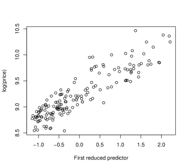
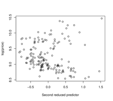
Figure 2: The scatter plots of $\log$(price) versus the first two reduced predictors

Iterative Hessian Transformation Method for Estimating the Central Mean Subspace (CMS)

In this section, we provide a summary of the main features of the iterative Hessian transformation (IHT) method proposed by Cook and Li (2002) for estimating the central mean subspace (CMS) in regression analysis.

Let $\{Y_{i},\mathbf{X}_{i}\}_{i=1}^{n}$ be an iid sample of size $n$ from the variables $(Y,\mathbf{X})$, where $\mathbf{X}$ is a $p$-dimensional predictor vector and $Y$ denotes the univariate response variable. We define $\mathbf{Z}=\boldsymbol{\Sigma}^{-1/2}_{xx}(\mathbf{X}-E[\mathbf{X}])$, where $\boldsymbol{\Sigma}_{xx}=\text{cov}(\mathbf{X})$ is assumed to be positive definite. The relationship between the central mean subspace (CMS) obtained based on the original predictors and the standardized predictors is given by $\mathcal{S}_{E[Y|\mathbf{X}]}=\boldsymbol{\Sigma}^{-1/2}_{xx}\mathcal{S}_{E[Y|\mathbf{Z}]}$ Cook and Li (2002). The following lemma, known as Theorem 3 in Cook and Li (2002), forms the foundation of the IHT method.

Lemma 3

Suppose $E[\mathbf{Z}|\boldsymbol{\eta}^{T}\mathbf{Z}]$ is linear in $\mathbf{Z}$ and $U$ and $V$ are measurable functions of $\boldsymbol{\eta}^{T}\mathbf{Z}$ such that $(UY+V)\mathbf{Z}$ is integrable. Then, $E\{(UY+V)\mathbf{Z}\}\in\mathcal{S}_{E[Y|\mathbf{Z}]}$.

This lemma presents an approach to generate basis vectors for constructing the CMS. These vectors, known as COZY vectors, capture the covariance between $\mathbf{Z}$ and the transformed response $Y^{\star}=(UY+V)$. Further details can be found in Cook and Li (2002). Setting $U=1$ and $V=0$, we have $E[(UY+V)]\mathbf{Z}]=\boldsymbol{\Gamma}_{yz}$ with probability 1, as stated in Lemma 3. Furthermore, under condition C.1 in Theorem 1 in Cook and Li (2002), we have $\boldsymbol{\Gamma}_{yz}\in\mathcal{S}_{E[Y|\mathbf{Z}]}$. Hence, an estimator for the CMS can be derived based on the $\boldsymbol{\Gamma}_{yz}$. Lemma 4 (Proposition 3 in Cook and Li, 2002) provides the detailed estimation procedure for the CMS, known as the iterative Hessian transformation (IHT) method. The following lemma restates Proposition 3 from Cook and Li (2002).

Lemma 4

Suppose $\mathbf{M}\in\mathbb{R}^{p\times p}$ is a matrix and $\boldsymbol{\Gamma}\in\mathbb{R}^{p}$ is a vector. For any $s>r$, if $~{}~{}\mathbf{M}^{r}\boldsymbol{\Gamma}\subset Span(\boldsymbol{\Gamma},\mathbf{M}\boldsymbol{\Gamma},\cdots,\mathbf{M}^{r-1}\boldsymbol{\Gamma})$, then, we have $\mathbf{M}^{s}\boldsymbol{\Gamma}\subset Span(\boldsymbol{\Gamma},\mathbf{M}\boldsymbol{\Gamma},\cdots,\mathbf{M}^{r-1}\boldsymbol{\Gamma})$.

Suppose $\boldsymbol{\Sigma}_{yzz}=E[Y\mathbf{Z}\mathbf{Z}^{T}]$. According to Corollary 2 in Cook and Li (2002), we have $Span\{\boldsymbol{\Sigma}^{j}_{yzz}\boldsymbol{\Gamma}_{yz};~{}j=0,1,\dots\}\in\mathcal{S}_{E[Y|\mathbf{Z}]}$, which has dimension $d$. By applying Lemma 4, we can find an integer $s\leq d$ such that the first $s$ vectors in the sequence, $\boldsymbol{\Gamma}_{yz},\boldsymbol{\Sigma}_{yzz}\boldsymbol{\Gamma}_{yz},\dots,\boldsymbol{\Sigma}_{yzz}^{s-1}\boldsymbol{\Gamma}_{yz}$, are linearly independent, and all the remaining vectors are linearly dependent on the sequence $\boldsymbol{\Gamma}_{yz},\boldsymbol{\Sigma}_{yzz}\boldsymbol{\Gamma}_{yz},\dots,\boldsymbol{\Sigma}_{yzz}^{s-1}\boldsymbol{\Gamma}_{yz}$. To compute the first $p$ COZY vectors, we set $U=1$ and $V=0$. Each COZY vector is then assigned as a column in the matrix $\mathbf{M}=(\boldsymbol{\Gamma}_{yz},\boldsymbol{\Sigma}_{yzz}\boldsymbol{\Gamma}_{yz},\dots,\boldsymbol{\Sigma}_{yzz}^{p-1}\boldsymbol{\Gamma}_{yz})$, which forms a $p\times p$ matrix. Then, we define the matrix $\boldsymbol{\Psi}=\mathbf{MM}^{T}$, and perform the eigenvector and eigenvalue decomposition on $\boldsymbol{\Psi}$. The leading $d$ eigenvectors of $\boldsymbol{\Psi}$, corresponding to the $d$ largest eigenvalues, serve as the estimated basis for the CMS, $\mathcal{S}_{E[y|\mathbf{z}]}$.

Consider an iid sample $\{Y_{i},\mathbf{X}_{i}\}_{i=1}^{n}$ and let $\mathbf{Z}$ represent the standardized predictors. Let $\widehat{\mathbf{M}}$ be the sample version of $\mathbf{M}=(\boldsymbol{\Gamma}_{yz},\boldsymbol{\Sigma}_{yzz}\boldsymbol{\Gamma}_{yz},\dots,\boldsymbol{\Sigma}_{yzz}^{p-1}\boldsymbol{\Gamma}_{yz})$. Then, the following steps outline the estimation process of the CMS using the IHT method Cook and Li (2002).

1. Compute the $p$-dimensional COZY vectors: $\widehat{\boldsymbol{\Gamma}}_{{y}{z}},\widehat{\boldsymbol{\Sigma}}_{{y}{z}{z}}\widehat{\boldsymbol{\Gamma}}_{{y}{z}},\dots,\widehat{\boldsymbol{\Sigma}}_{{y}{z}{z}}^{p-1}\widehat{\boldsymbol{\Gamma}}_{{y}{z}}$ using the following formulas

   $$\begin{split}\widehat{\boldsymbol{\Sigma}}_{yzz}&=\frac{1}{n}\sum_{i=1}^{n}y_{i}\mathbf{ZZ}^{T},~{}~{}~{}~{}\widehat{\boldsymbol{\Gamma}}_{yz}=\frac{1}{n}\sum_{i=1}^{n}y_{i}\mathbf{Z},\end{split}$$ (25)

   where $\mathbf{Z}=\widehat{\boldsymbol{\Sigma}}_{xx}^{-1/2}(\mathbf{X}-\overline{\mathbf{X}})$, and $\widehat{\boldsymbol{\Sigma}}_{xx}$ and $\overline{\mathbf{X}}$ are the sample covariance matrix and the sample mean of $\mathbf{X}$, respectively.

2. Calculate the $p\times p$ matrix $\widehat{\mathbf{M}}=(\widehat{\Gamma}_{{y}{z}},\widehat{\boldsymbol{\Sigma}}_{{y}{z}{z}}\widehat{\Gamma}_{{y}{z}},\cdots,\widehat{\boldsymbol{\Sigma}}_{{y}{z}{z}}^{p-1}\widehat{\Gamma}_{{y}{z}})$, and compute $\widehat{\boldsymbol{\Psi}}=\widehat{\mathbf{M}}\widehat{\mathbf{M}}^{T}$.

3. Perform a spectral decomposition of matrix $\widehat{\boldsymbol{\Psi}}$. Let $(\widehat{\mathbf{e}}_{1},\widehat{\lambda}_{1}),\cdots,(\widehat{\mathbf{e}}_{d},\widehat{\lambda}_{d})$ be the first $d$ leading eigenvectors-eigenvalue pairs, where $\widehat{\lambda}_{1}\geq\cdots\geq\widehat{\lambda}_{d}\geq 0=\cdots=0.$

4. The estimated CMS is given by $\widehat{\mathcal{S}}_{E[Y|\mathbf{X}]}=Span\{\widehat{\boldsymbol{\Sigma}}_{xx}^{-1/2}\widehat{\mathbf{e}}_{1},\dots,\widehat{\boldsymbol{\Sigma}}_{xx}^{-1/2}\widehat{\mathbf{e}}_{d}\}$ where $\widehat{\boldsymbol{\Sigma}}_{xx}$ is the sample covariance matrix.

Algorithm 4 IHT method for Estimating the CMS

R Function for Iterative Hessian Transformation Method

The itdr() function in our itdr package facilitates the estimation of the central mean subspace by using the IHT method. The following R code demonstrates the process of estimating the CMS on the Recumbent cows dataset, which was collected at the Ruakura (N. Z.) and analyzed by Clark et al. (1987). We have used the same response variables and predictor variables as Cook and Li (2002). Specifically, the predictors are $\log(AST)$ (logarithm of serum aspartate aminotransferase in U/l at 30C); $log(CK)$ (logarithm of serum creatine phosphokinase in U/l at 30C); and $\log(UREA)$ (logarithm of serum urea in mmol/l). The response variable is a binary variable, where $Y=1$ indicates surviving cows, and $Y=0$ indicates not surviving cows.

    library(itdr)    data("Recumbent")    Recumbent.df=na.omit(Recumbent)    y=Recumbent.df$outcome    X1=log(Recumbent.df$ast)    X2=log(Recumbent.df$ck)    X3=log(Recumbent.df$urea)    x=matrix(c(X1,X2,X3),ncol=3)    fit.iht_CMS=itdr(y,x,d = 2,method="iht")    fit.iht_CMS$eta_hatThe itdr() function has the following arguments for the IHT method: $\mathbf{Y}$ is a vector of $n$ observations on the response variable, $\mathbf{X}$ is the predictor matrix of dimension $n\times p$, $d$ is the dimension of the central mean subspace, and the method argument takes “iht” to indicate the use of the IHT method.

               [,1]        [,2]    [1,]  0.3260269  0.95986216    [2,] -0.2395713 -0.27884564    [3,] -0.9145010  0.03016189

The output displayed above illustrates the estimated basis vectors for the CMS of the Recumbent cows dataset.

Fourier Transformation Method for Inverse Dimension Reduction in Multivariate Regression

In this section, we present a summary of the theoretical framework of the Fourier transformation method for inverse dimension reduction (invFM) proposed by Weng and Yin (2018). This method aims to estimate the central subspace (CS). We consider an iid sample $\{\mathbf{Y}_{i},\mathbf{X}_{i}\}$, $i=1,\dots,n$, from $(\mathbf{Y},\mathbf{X})$, where $\mathbf{Y}\in\mathbb{R}^{q}$ represents a $q$-dimensional response variable, $\mathbf{X}\in\mathbb{R}^{p}$ is a $p$-dimensional predictor variable, and $n$ is the sample size. Furthermore, we assume that $\mathbf{Z}$ represents the standardized version of the predictor $\mathbf{X}$, defined as $\mathbf{Z}=\boldsymbol{\Sigma}^{-1/2}(\mathbf{X}-\boldsymbol{\mu})$, where $\boldsymbol{\mu}$ and $\boldsymbol{\Sigma}$ are the mean and covariance matrix of $\mathbf{X}$, respectively. Under the linearity condition, it can be shown that $m(\mathbf{y})=E[\mathbf{Z}|\mathbf{Y}=\mathbf{y}]\in\mathcal{S}_{\mathbf{Y}|\mathbf{Z}}$ Cook (1998). Let $f(\mathbf{y})$ denote the marginal distribution of $\mathbf{Y}$ and let $\boldsymbol{\omega}\in\mathbb{R}^{q}$. According to Weng and Yin (2018), the Fourier transformation of the density-weighted $m(\mathbf{y})$ is given by

$$\boldsymbol{\psi}(\boldsymbol{\omega})=\int\exp\{i\boldsymbol{\omega}^{T}\mathbf{y}\}m(\mathbf{y})f(\mathbf{y})d\mathbf{y}.$$ (26)

For more comprehensive information regarding the Fourier transformation, see Folland (1992). Using simple algebra, we can show that $\boldsymbol{\psi}(\boldsymbol{\omega})=E[\exp\{i\boldsymbol{\omega}^{T}\mathbf{y}\}\mathbf{Z}]$, and $\mathcal{S}_{E[\mathbf{Z}|\mathbf{Y}]}=Span\left\{\boldsymbol{\psi}(\boldsymbol{\omega});\boldsymbol{\omega}\in\mathbb{R}^{q}\right\}$. Moreover, under the linearity condition, $\mathcal{S}_{E[\mathbf{Z}|\mathbf{Y}]}$ can be expressed as $Span\left\{m(\mathbf{y}),\mathbf{y}\in supp(f(\mathbf{y}))\right\}=Span\left\{m(\mathbf{y})f(\mathbf{y}),\mathbf{y}\in supp(f(\mathbf{y}))\right\}\subseteq\mathcal{S}_{\mathbf{Y}|\mathbf{Z}}$. Consequently, by employing the inverse Fourier transformation provided in Folland (1992), we can recover the density-weighted conditional mean function $m(\mathbf{y})$ from $\psi(\boldsymbol{\omega})$, as follows

$$m(\mathbf{y})f(\mathbf{y})=\frac{1}{2\pi}\int\exp\{-i\boldsymbol{\omega}^{T}\mathbf{y}\}\boldsymbol{\psi}(\boldsymbol{\omega})d\boldsymbol{\omega}.$$ (27)

Hence, we have $\mathcal{S}_{E[\mathbf{Z}|\mathbf{Y}]}=Span\{\boldsymbol{\psi}(\boldsymbol{\omega});\boldsymbol{\omega}\in\mathbb{R}^{q}\}=Span\{a(\boldsymbol{\omega}),b(\boldsymbol{\omega});\boldsymbol{\omega}\in\mathbb{R}^{q}\}$ where $\mathbf{a}(\boldsymbol{\omega})$ and $\mathbf{b}(\boldsymbol{\omega})$ are the real and imaginary parts of $\boldsymbol{\psi}(\boldsymbol{\omega})$, respectively.

According to the preceding discussion, the Fourier transform expression $\boldsymbol{\psi}(\boldsymbol{\omega})$ does not explicitly contain the mean function $m(\mathbf{y})$. Consequently, $\boldsymbol{\psi}(\boldsymbol{\omega})$ can be estimated without directly estimating $m(\mathbf{y})$. That is, we can find an estimator for the CS by calculating $\boldsymbol{\psi}(\boldsymbol{\omega})$ for a given set of $q$-dimensional vectors $\{\boldsymbol{\omega}_{r}\}_{r=1}^{k}$, where $k$ is a prespecified number. Based on Proposition 2.1 in Weng and Yin (2018), there exists a finite sequence of $\boldsymbol{\omega}_{r}\in\mathbb{R}^{q}$, $r=1,\dots,k$, such that $\mathcal{S}_{E[\mathbf{Z}|\mathbf{Y}]}=Span\{\mathbf{a}(\boldsymbol{\omega}_{1}),\mathbf{b}(\boldsymbol{\omega}_{1}),\dots,\mathbf{a}(\boldsymbol{\omega}_{k}),\mathbf{b}(\boldsymbol{\omega}_{k})\}$. Therefore, we utilize $\boldsymbol{\psi}(\boldsymbol{\omega}_{r})$s to derive a candidate matrix that targets the CS. We construct a nonnegative definite symmetric dimension reduction matrix $\mathbf{V}\in\mathbb{R}^{p\times p}$ using $\boldsymbol{\psi}(\boldsymbol{\omega}_{r})$, $r=1,\dots,k$, which is referred to as a kernel dimension reduction matrix. Then, we perform the eigen decomposition of a sample version of $\mathbf{V}$, denoted as $\widehat{\mathbf{V}}$. Finally, the first $d$ leading eigenvectors corresponding to the foremost $d$ leading eigenvalues of $\widehat{\mathbf{V}}$ form an orthogonal basis for the CS.

Algorithm of the invFM

Let $\{\boldsymbol{\omega}_{r}\}_{r=1}^{k}$ be a predefined set of $q$-dimensional vectors, $(\mathbf{Y}_{i},\mathbf{X}_{i})$, $i=1,\dots,n$, be a random sample of size $n$, where $\mathbf{Y}_{i}\in\mathbb{R}^{q}$, and $\mathbf{X}_{i}\in\mathbb{R}^{p}$. Suppose $\boldsymbol{\Omega}=(\mathbf{a}(\boldsymbol{\omega}_{1}),\mathbf{b}(\boldsymbol{\omega}_{1}),\cdots,\mathbf{a}(\boldsymbol{\omega}_{k}),\mathbf{b}(\boldsymbol{\omega}_{k}))$, for $k>0$, and let $\mathbf{V}=\boldsymbol{\Omega}\boldsymbol{\Omega}^{T}$ represent the population version of the kernel dimension reduction matrix, and assume the dimension $d=dim(\mathcal{S}_{E(\mathbf{Z}|\mathbf{Y})})$ is known. Then, the following standard steps are used to estimate the central subspace based on the Fourier transformation method for inverse dimension reduction.

1. Standardize the predictors by computing $\widehat{\mathbf{z}}_{i}=\widehat{\boldsymbol{\Sigma}}^{-1/2}(\mathbf{x}_{i}-\overline{\mathbf{x}})foreachobservationi=1,\dots,n$, where $\overline{\mathbf{x}}$ and $\widehat{\boldsymbol{\Sigma}}$ are the sample mean and the sample covariance matrix of $\mathbf{X}$, respectively.

2. Choose a random sequence of $\{\boldsymbol{\omega}_{r}\}_{r=1}^{k}$ from a normal distribution and compute the sample version of $\boldsymbol{\psi}(\boldsymbol{\omega}_{r})$ using the formula:

   $$\widehat{\boldsymbol{\psi}}(\boldsymbol{\boldsymbol{\omega}_{r}})=n^{-1}\sum_{i=1}^{n}\exp\{i\boldsymbol{\boldsymbol{\omega}_{r}^{T}\mathbf{y}_{i}}\}\widehat{\mathbf{z}}_{i},$$ (28)

   calculate the real and imaginary parts as $\widehat{\mathbf{a}}(\boldsymbol{\omega_{r}})=Real\{\widehat{\boldsymbol{\psi}}(\boldsymbol{\omega}_{r})\}$ and $\widehat{\mathbf{b}}(\boldsymbol{\omega}_{r})=Imag\{\widehat{\boldsymbol{\psi}}(\boldsymbol{\omega_{r}})\}$.

3. Construct $\widehat{\boldsymbol{\Omega}}$ and $\widehat{\mathbf{V}}$ as follows

   $$\widehat{\boldsymbol{\Omega}}=\{\widehat{\boldsymbol{a}}(\boldsymbol{\omega}_{r}),\widehat{\boldsymbol{b}}(\boldsymbol{\omega}_{r})\}_{r=1}^{k},~{}~{}~{}\widehat{\mathbf{V}}=\widehat{\boldsymbol{\Omega}}\widehat{\boldsymbol{\Omega}}^{T},$$ (29)

   where $\widehat{\boldsymbol{\Omega}}$ is a $p\times 2k$ matrix and $\widehat{\mathbf{V}}$ is a $p\times p$ sample kernel dimension reduction matrix.

4. Perform eigen decomposition of $\widehat{\mathbf{V}}$ and select the first $d$ leading eigenvectors $(\widehat{\boldsymbol{\eta}_{i}},i=1,\dots,d)$ corresponding to the $d$ largest eigenvalues $\widehat{\lambda}_{1}\geq\cdots\geq\widehat{\lambda}_{d}$ as the estimated basis of $\mathcal{S}_{E[\mathbf{Z}|\mathbf{Y}]}$.

5. Back transform the eigenvectors to the original scale of $\mathbf{X}$. Compute $\widehat{\boldsymbol{\beta}}_{i}=\widehat{\boldsymbol{\Sigma}}^{-1/2}\widehat{\boldsymbol{\eta}}_{i},~{}~{}i=1,\dots,d$.

Algorithm 5 Fourier transformation method

The above steps are standard in SDR procedures except Step 3, which employs the proposed invFM method. In the case of a univariate response, select scalar values for $\omega_{r}$, i.e., $\omega_{r}\in\mathbb{R}$.

Dimension Selection of the Central Subspace using invFM Method

In the previous section, we made the assumption that the dimension $d$ of the central subspace (CS) is already known. In this section, we describe a testing procedure to select the appropriate dimension. Let us consider a hypothetical dimension $m$ for the CS, and formulate the null hypothesis ($H_{0}$) and alternative hypothesis ($H_{a}$) as follows:

$$H_{0}:d=m~{}~{}~{}~{}\text{versus}~{}~{}~{}~{}H_{a}:d>m.$$ (30)

Weng and Yin (2018) proposed a weighted chi-square test statistic to test the hypothesis in Equation (30). This statistic, denoted as $\widehat{\Lambda}_{m}$, is defined as

$$\widehat{\Lambda}_{m}=n\sum_{j=m+1}^{p}\widehat{\lambda}_{j}.$$ (31)

The value of $m$ begins at $m=0$, and continues to increase by one until the null hypothesis at the current value of $m$ cannot be rejected. Moreover, a scaled test statistic suggested by Bentler and Xie (2000) as a simplified version of the weighted chi-square test, can be used to determine the dimension. The scaled test statistic is defined as

$$\overline{T}_{m}=[\text{trace}(\widehat{\mathbf{V}})/p^{\star}]^{-1}n\sum_{j=m+1}^{p}\widehat{\lambda}_{j}\sim\chi^{2}_{p^{\star}},$$ (32)

where $\widehat{\mathbf{V}}$ is a consistent estimator of $\mathbf{V}$, and is defined in Equation (29), and $p^{\star}=(p-m)(2k-m)$. Another test statistic that can be employed to test the hypotheses in Equation (30) is the adjusted test statistic proposed by Bentler and Xie (2000), defined as

$$\widetilde{T}_{m}=[\text{trace}(\widehat{\mathbf{V}})/s^{\star}]^{-1}n\sum_{j=m+1}^{p}\widehat{\lambda}_{j}\sim\chi^{2}_{s^{\star}},$$ (33)

where $s^{\star}=[\text{trace}(\widehat{\mathbf{V}})]^{2}/\text{trace}(\widehat{\mathbf{V}}^{2})$, and $\widehat{\mathbf{V}}$ is defined in Equation (29).

R Functions for Fourier Method for Inverse Dimension Reduction in Multivariate Regression

In this section, we demonstrate the usage of functions included in our itdr package to perform the Fourier transformation method for the inverse dimension reduction proposed by Weng and Yin (2018). The first subsection illustrates the process of selecting the dimension of the central subspace (CS) using the “2015 Planning Database” (PDB) dataset which is available in our itdr package. More details of this dataset can be found at https://www.census.gov/data/datasets/2015/adrm/research/2015-planning-database.html. The main function for estimating the central subspace is described in the second subsection.

R Function for Determining the Dimension of the Central Subspace (CS)

Within our $\mathbf{itdr}$ package, the d.test() function calculates the $p$-values for three different test statistics defined in Equations (31)-(33). These include the weighted chi-square test statistic $\widehat{\Lambda}_{m}$, the scaled test statistic $\overline{T}_{m}$, and the adjusted test statistic $\widetilde{T}_{m}$.

We utilize the same dataset employed by Weng and Yin (2018), which consists of the 2010 Census and 2009-2013 American Community Survey data, This dataset encompasses housing, demographic, socioeconomic, and Census operational information at the block-group level. Any observations with missing values are excluded. Then, the Box-Cox transformation is applied to the predictors to ensure adherence to the linearity condition.

    library(itdr)    data(PDB)    colnames(PDB)=NULL    p=15    set.seed(123)    df=PDB[,c(79,73,77,103,112,115,124,130,132,145,149,151,153,155,167,169)]    dff=as.matrix(df)    #remove the NA rows    planingdb=dff[complete.cases(dff),]    y=planingdb[,1] #n-dimensionl response vector    x=planingdb[,c(2:(p+1))] # raw design matrix    x=x+0.5    # design matrix after transformations    xt=cbind(x[,1]^(.33),x[,2]^(.33),x[,3]^(.57),x[,4]^(.33),x[,5]^(.4),    x[,6]^(.5),x[,7]^(.33),x[,8]^(.16),x[,9]^(.27),x[,10]^(.5),    x[,11]^(.5),x[,12]^(.33),x[,13]^(.06),x[,14]^(.15),x[,15]^(.1))    #run the hypothesis tests    d.test(y,x,m=1)The d.test() function takes the following arguments: $\mathbf{Y}$, a vector of $n$ observations; $\mathbf{X}$, a predictor matrix of dimension $n\times p$; and $m$, the assumed dimension of the central subspace.

     Hypothesis Tests for selecting sufficient dimension (d)     Null: d=m vs Alternative: d>m     Test  W.Ch.Sq Scaled     Adjusted     p-value  0.9837  1       0.9306314The above output displays the $p$-values for the three different tests introduced in Equations (31)-(33). Starting with $m=1$, if the p-value is below a significant level, the null hypothesis is rejected, and the test proceeds to the next value of $m$. If the p-value is above the significant level, the null hypothesis is not rejected, and the test is stopped. According to the results, all $p$-values from the three different tests are greater than $0.05$. Therefore, we can assume the hypothetical dimension, i.e., $m=1$, represents the true dimension of the CS in the PDB dataset, that is, $\widehat{d}=1$.

R Function for Estimating the Central Subspace (CS)

The invFM() function in our itdr package provides an estimator for the CS using the Fourier transformation method for the inverse dimension reduction proposed by Weng and Yin (2018). Similar to the previous section, we utilize the same response variable and the predictor variable with the same Box-Cox transformations as described in Weng and Yin (2018) on the PDB dataset. The following R code illustrates the usage of the invFM() function.

    set.seed(123)    W=sapply(100,rnorm)    # estimated dimension of the CS from Section 4.1    betahat <-invFM(x = xt, y = y, d = 1, w = W, x_scale = F)$beta    #estimated basis    betahat    plot(y ~ xt %*% betahat, xlab = "First reduced predictor",    ylab = "Health insurance coverage")

 [1] -0.14791302 -0.25891444 -0.61782407 -0.10608213 -0.07648674 -0.48468920 [7] -0.02378407  0.05098216 -0.06333981 -0.35316016 -0.27668059 -0.24190026[13] -0.09364571 -0.03655110 -0.01670101 The invFM() function accepts the following arguments: $\mathbf{X}$, the predictor matrix of dimension $n\times p$; $\mathbf{Y}$, the response matrix of dimension $n\times q$; $d$, the dimension of the central subspace; $W$, a prespecified matrix of $\{\boldsymbol{\omega}_{r}\}$s of dimension $q\times k$; and x_scale, a logical parameter that specifies whether the predictor matrix should be normalized or not, with the ”TRUE“ as the default.

The provided output displays the estimated single-index direction $\hat{\boldsymbol{\beta}}\in\mathbb{R}^{15\times 1}$ for the central subspace of the PDB dataset. Based on the scatter plot presented in Figure 3, it can be observed that there exists a negative correlation between health insurance coverage and the first reduced predictor. Specifically, as the value of the first reduced predictor increases, the health insurance coverage tends to decrease. This finding suggests that the first reduced predictor holds potential significance as a predictor variable in the model, and further investigation is warranted.

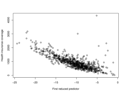
Figure 3: The scatter plot of $Y$: health insurance coverage versus the first reduced predictor

A Minimum Discrepancy Approach using Fourier Transformation

In this section, we provide an overview of a family of optimal estimators that optimize a quadratic function using the Fourier transformation approach introduced by (Weng and Yin, 2022). Given a finite sequence $\{\boldsymbol{\omega}_{r}\}\in R^{q},r=1,\ldots,k$, we define $\boldsymbol{\xi}_{r}=\boldsymbol{\Sigma}^{-1}[E(e^{i\boldsymbol{\omega}^{T}_{r}\mathbf{Y}}\mathbf{X})-E(e^{i\boldsymbol{\omega}^{T}_{r}\mathbf{Y}})E(\mathbf{X})]\in\mathbb{C}^{p}$. According to Weng and Yin (2018), we have $\boldsymbol{\xi}_{r}\in\mathcal{S}_{\mathbf{Y}|\mathbf{X}}$. We denote the real and imaginary parts of a complex vector with superscripts $R$ and $I$, respectively, and we represent $\boldsymbol{\xi}$ as a matrix $\boldsymbol{\xi}=\left(\boldsymbol{\xi}^{R}_{r},\boldsymbol{\xi}^{I}_{r}\right)^{k}_{r=1}$, combining each $\boldsymbol{\xi}^{R}_{r}$ and $\boldsymbol{\xi}^{I}_{r}$. Hence, the column space spanned by $\boldsymbol{\xi}$ is within the central subspace: $Span(\boldsymbol{\xi})\subseteq\mathcal{S}_{\mathbf{Y}|\mathbf{X}}$.

Assume $\{\mathbf{y}_{j},\mathbf{x}_{j}\}$, for $j=1,\ldots,n$, are independent and identically distributed (iid) samples of $(\mathbf{Y},\mathbf{X})$. Let $\bar{\mathbf{x}}$ be the sample mean of $\mathbf{X}$ and

$$\hat{\boldsymbol{\xi}}_{r}=\hat{\boldsymbol{\Sigma}}^{-1}\left(\frac{1}{n}\sum^{n}_{j=1}e^{i\boldsymbol{\omega}^{T}_{r}\mathbf{y}_{j}}\mathbf{x}_{j}-\frac{1}{n}\sum^{n}_{j=1}e^{i\boldsymbol{\omega}^{T}_{r}\mathbf{y}_{j}}\bar{\mathbf{x}}\right)$$

denote the sample estimate of $\boldsymbol{\xi}_{r}$. Then, $\hat{\boldsymbol{\xi}}=\left(\hat{\boldsymbol{\xi}}^{R}_{r},\hat{\boldsymbol{\xi}}^{I}_{r}\right)^{k}_{j=r}$ serves as a sample estimate of $\boldsymbol{\xi}$. We define the quadratic discrepancy function (QDF) of $\boldsymbol{\Gamma}\in\mathbb{R}^{p\times d}$ and $\mathbf{C}\in\mathbb{R}^{d\times 2k}$, with respect to the inner product matrix $\mathbf{V}$, as:

$$F_{d}(\boldsymbol{\Gamma},\mathbf{C};\mathbf{V})=[\text{vec}(\hat{\boldsymbol{\xi}})-\text{vec}(\boldsymbol{\Gamma}\mathbf{C})]^{T}\mathbf{V}[\text{vec}(\hat{\boldsymbol{\xi}})-\text{vec}(\boldsymbol{\Gamma}\mathbf{C})],$$ (34)

where $\text{vec}(\mathbf{A})$ is the vectorization of a matrix $\mathbf{A}$. The estimation of the central subspace can be achieved by minimizing the objective function $F_{d}(\boldsymbol{\Gamma},\mathbf{C};\mathbf{V})$, where $\boldsymbol{\Gamma}$ represents an orthogonal basis of the central subspace, $\mathbf{C}$ denotes the coordinates of the data points relative to the basis, and $\mathbf{V}$ is an inner product matrix. The accuracy of the resulting estimator heavily depends on the choice of $\mathbf{V}$. To shed light on this issue, Weng and Yin (2022) conducted an investigation into the effects of five different $\mathbf{V}$ matrices on the estimator and its properties. The final estimate $(\hat{\boldsymbol{\Gamma}},\hat{\mathbf{C}})$ is obtained by minimizing the objective function and provides an estimate of the central subspace and the corresponding coordinates of the data points.

1. The Fourier transform Inverse Regression Estimator (FT-IRE) is an optimal estimator that achieves asymptotic efficiency without any constraints or strong assumptions. To construct the inner product matrix $\boldsymbol{V}$, we begin by considering the population residual $\epsilon_{r}=e^{i\boldsymbol{\omega}^{T}_{r}\mathbf{Y}}-Ee^{i\boldsymbol{\omega}^{T}_{r}\mathbf{Y}}-\mathbf{Z}^{T}E(e^{i\boldsymbol{\omega}^{T}_{r}\mathbf{Y}}\mathbf{Z})$ obtained from an ordinary least squares fit of $e^{i\boldsymbol{\omega}^{T}_{r}\mathbf{Y}}$ on $\mathbf{Z}$. Furthermore, $\boldsymbol{\epsilon}=\left(\epsilon_{1}^{R},\epsilon_{1}^{I},\ldots,\epsilon_{k}^{R},\epsilon_{k}^{I}\right)^{T}$ consists of both the real and imaginary parts. As a result, we have

$$\sqrt{n}[\text{vec}(\hat{\boldsymbol{\xi}})-\text{vec}(\boldsymbol{\xi})]\overset{D}{\rightarrow}{N}(\mathbf{0},\boldsymbol{\Sigma}_{\boldsymbol{\xi}}),$$

where $\boldsymbol{\Sigma}_{\boldsymbol{\xi}}=\text{cov}\{\text{vec}[\boldsymbol{\Sigma}^{-1/2}\mathbf{Z}\boldsymbol{\epsilon}^{T}]\}\in\mathbb{R}^{2kp\times 2kp}$ is the limiting covariance matrix, and $\overset{D}{\rightarrow}$ denotes the convergence in distribution. When implementing the information matrix $\boldsymbol{V}={\boldsymbol{\Sigma}_{\boldsymbol{\xi}}}^{-1}$ to the QDF in Equaiton (34), the resulting minimizer, denoted as $\hat{\boldsymbol{\Gamma}}$, is the FT-IRE.

2. When the value of $k$ becomes too large, FT-IRE may encounter a singular limiting covariance matrix. To address this limitation, Weng and Yin (2022), proposed a technique where they construct multiple QDFs, each with its own limiting covariance matrix, treating them as independent entities. Specifically, they utilized several sequences of $\boldsymbol{\omega}^{(l)}\in R^{k_{l}},$ with $\sum k_{l}=k,l=1,\ldots,s$ and construct $s$ QDFs with the corresponding limiting covariance matrix $\boldsymbol{\Sigma}_{\boldsymbol{\xi}}^{(l)}\in R^{2pk_{l}\times 2pk_{l}}$. The degenerated QDF is defined as the summation of these $s$ QDFs, that is,

$$F_{d}(\boldsymbol{\Gamma},\mathbf{C};\{\boldsymbol{\Sigma}_{\boldsymbol{\xi}}^{(l)}\})=\sum^{s}_{l=1}[\text{vec}(\hat{\boldsymbol{\xi}}_{l})-\text{vec}(\boldsymbol{\Gamma}\mathbf{C}_{l})]^{T}\boldsymbol{\Sigma}_{\boldsymbol{\xi}}^{(l)}[\text{vec}(\hat{\boldsymbol{\xi}}_{l})-\text{vec}(\boldsymbol{\Gamma}\mathbf{C}_{l})].$$ (35)

This expression is equivalent to Equation (34) but employs a new inner product matrix $\mathbf{V}=\hat{\boldsymbol{\Gamma}}_{D}^{-1}=\text{diag}(\{\hat{\boldsymbol{\Sigma}}_{l}^{(l)-1}\})$. The degenerated estimator $\hat{\boldsymbol{\Gamma}}$, which minimizes (35), is referred to as the Fourier transform degenerated inverse regression estimator (FT-DIRE).

3. Weng and Yin (2022) proved that the invFM estimator is sub-optimal when employing a special inner product matrix $\mathbf{V}=\text{diag}\{\hat{\boldsymbol{\Sigma}}\}$ in the QDF function (34). The corresponding special QDF can be expressed as follows:

$$\begin{array}[]{ccl}F_{d}(\boldsymbol{\Gamma},\mathbf{C};\text{diag}\{\hat{\boldsymbol{\Sigma}}\})&=&[\text{vec}(\hat{\boldsymbol{\xi}})-\text{vec}(\boldsymbol{\Gamma}\mathbf{C})]^{T}\text{diag}\{\hat{\boldsymbol{\Sigma}}\}[\text{vec}(\hat{\boldsymbol{\xi}})-\text{vec}(\boldsymbol{\Gamma}\mathbf{C})]\\ &=&\sum_{l=1}^{2k}(\hat{\boldsymbol{\xi}}_{l}-\boldsymbol{\Gamma}\mathbf{C}_{l})^{T}\hat{\boldsymbol{\Sigma}}(\hat{\boldsymbol{\xi}}_{l}-\boldsymbol{\Gamma}\mathbf{C}_{l}).\\ \end{array}$$ (36)

In this formulation, each column of $\boldsymbol{\xi}$ is considered independent of the other. The FT-SIRE is theoretically equivalent to the invFM estimator proposed by Weng and Yin (2018). The minimizer of (36), denoted as Fourier transform special inverse regression estimator (FT-SIRE), is represented by $\hat{\boldsymbol{\Gamma}}$.

4. Obtaining a consistent estimate of ${\boldsymbol{\Sigma}_{\boldsymbol{\xi}}}^{-1}$ requires considering fourth moments of the predictors. To achieve robust estimation, let us assume the covariance matrix $\boldsymbol{\Sigma}$ is known. Let $\tilde{\boldsymbol{\xi}}_{j}=\boldsymbol{\Sigma}^{-1}(\frac{1}{n}\sum^{n}_{j=1}e^{i\boldsymbol{\omega}^{T}_{r}\mathbf{y}_{j}}\mathbf{x}_{j}-\frac{1}{n}\sum^{n}_{j=1}e^{i\boldsymbol{\omega}^{T}_{r}\mathbf{y}_{j}}\bar{\mathbf{x}})$, and $\tilde{\epsilon}=e^{i\boldsymbol{\omega}^{T}\mathbf{Y}}-Ee^{i\boldsymbol{\omega}^{T}\mathbf{Y}}$. Furthermore, we define $\tilde{\boldsymbol{\xi}}=\left(\tilde{\boldsymbol{\xi}}^{R}_{r},\tilde{\boldsymbol{\xi}}^{I}_{r}\right)^{m}_{r=1}\in\mathbb{R}^{p\times 2m}$. Then, we have

$$\sqrt{n}[\text{vec}(\tilde{\boldsymbol{\xi}})-\text{vec}(\boldsymbol{\xi})]\overset{D}{\rightarrow}N(0,\tilde{\boldsymbol{\Sigma}}_{\tilde{\boldsymbol{\xi}}}),$$

where $\tilde{\boldsymbol{\Sigma}}_{\tilde{\boldsymbol{\xi}}}=(\mathbf{I}\otimes\boldsymbol{\Sigma}^{-1/2})\text{cov}[\text{vec}(\mathbf{Z}\tilde{\boldsymbol{\epsilon}}^{T})](\mathbf{I}\otimes\boldsymbol{\Sigma}^{-1/2})$ and $\tilde{\boldsymbol{\epsilon}}=(\tilde{\epsilon}_{1}^{R},\tilde{\epsilon}_{1}^{I},\ldots,\tilde{\epsilon}_{k}^{R},\tilde{\epsilon}_{k}^{I})^{T}$. Here, $\tilde{\epsilon}_{r}^{R}$ and $\tilde{\epsilon}_{r}^{I}$ are the real and imaginary parts, respectively, of $\tilde{\epsilon}_{r}$, for $r=1,\ldots,k$. The limiting covariance matrix, $\tilde{\boldsymbol{\Sigma}}_{\tilde{\boldsymbol{\xi}}}$, only requires the second moments of the predictor. Now, define the robust QDF as

$$F_{d}(\boldsymbol{\Gamma},\mathbf{C};\tilde{\mathbf{G}}^{-1})=[\text{vec}(\hat{\boldsymbol{\xi}})-\text{vec}(\boldsymbol{\Gamma}\mathbf{C})]^{T}\tilde{\mathbf{G}}^{-1}[\text{vec}(\hat{\boldsymbol{\xi}})-\text{vec}(\boldsymbol{\Gamma}\mathbf{C})],$$ (37)

where $\tilde{\mathbf{G}}=(\mathbf{I}\otimes\hat{\boldsymbol{\Sigma}}^{-1/2})\widehat{\text{cov}}[\text{vec}(\mathbf{Z}\tilde{\boldsymbol{\epsilon}}^{T})](\mathbf{I}\otimes\hat{\boldsymbol{\Sigma}}^{-1/2})$. The estimator that minimizes the robust QDF is called the Fourier transform robust inverse regression estimator (FT-RIRE). The inner product matrix $\mathbf{V}=\tilde{\mathbf{G}}^{-1}$ only needs second moments, making FT-RIRE more theoretically robust.

5. Similarly, we define a diagonal block inner product matrix as $\tilde{\mathbf{G}}_{D}^{-1}=\text{diag}\{\tilde{\mathbf{G}}_{1}^{-1},\ldots,\tilde{\mathbf{G}}_{s}^{-1}\}$, where $\tilde{\mathbf{G}}_{l}^{-1}$ is defined for each $\boldsymbol{\omega}^{(l)}\in R^{k_{l}},l=1,\ldots,s$. The degenerated robust estimator that minimizes $F_{d}(\boldsymbol{\Gamma},\mathbf{C};\tilde{\mathbf{G}}_{D}^{-1})$ is called the Fourier transform degenerated robust inverse regression estimator (FT-DRIRE).

1. Choose an initial value for $\boldsymbol{\Gamma}\in\mathbb{R}^{p\times d}$. One possible choices is to set $\boldsymbol{e}_{i}=(0,\cdots,0,1,0,\cdots,0)^{T}$ with the $i^{th}$ element equal to 1 and others equal to $0$. Alternatively, we use the Fourier transformation result from Weng and Yin (2018).

2. Fixed $\boldsymbol{\Gamma}$ and update $\mathbf{C}$ by minimizing $F_{d}(\boldsymbol{\Gamma},\mathbf{C};\mathbf{V})$. Fit a linear regression of $\mathbf{V}^{1/2}\text{vec}(\hat{\boldsymbol{\xi}})$ on $\mathbf{V}^{1/2}(\mathbf{I}_{2m}\otimes\boldsymbol{\Gamma})$, then obtain $\text{vec}(\mathbf{C})=[(\mathbf{I}_{2m}\otimes\boldsymbol{\Gamma}^{T})\mathbf{V}(\mathbf{I}_{2m}\otimes\boldsymbol{\Gamma})]^{-1}(\mathbf{I}_{2m}\otimes\boldsymbol{\Gamma}^{T})\mathbf{V}\text{vec}(\hat{\boldsymbol{\xi}})$.

3. Fixed $\mathbf{C}$ and minimize $F_{d}(\boldsymbol{\Gamma},\mathbf{C};\mathbf{V})$ with respect to one column of $\boldsymbol{\Gamma}$, subject to the unit norm and orthogonality to other columns (keeping them constant). For this partial minimization problem, use the quadratic discrepancy function: $F(\mathbf{b})=(\boldsymbol{\alpha}_{k}-(\mathbf{c}_{k}^{T}\otimes\mathbf{I}_{p})\mathbf{Q}_{\boldsymbol{\Gamma}_{(-k)}}\mathbf{b})^{T}\boldsymbol{V}(\boldsymbol{\alpha}_{k}-(\mathbf{c}_{k}^{T}\otimes\mathbf{I}_{p})\mathbf{Q}_{\boldsymbol{\Gamma}_{(-k)}}\mathbf{b})$, where $\boldsymbol{\alpha}_{k}=\text{vec}(\hat{\boldsymbol{\xi}}-\boldsymbol{\Gamma}_{(-k)}\mathbf{C}_{(-k)})$, $\mathbf{c}_{k}$ is $k^{th}$ column of $\mathbf{C}$, $\mathbf{C}_{(-k)}$ (or $\boldsymbol{\Gamma}_{(-k)}$) is the matrix by deleting the $k^{th}$ column from $\mathbf{C}$ (or $\boldsymbol{\Gamma}$), and $\mathbf{Q}_{\boldsymbol{\Gamma}_{(-k)}}$ is orthogonal complement of Span$(\boldsymbol{\Gamma}_{(-k)})$. Repeat the following steps for $k=1,...,d$:

   1. Let $\boldsymbol{\Gamma}=(\mathbf{b}_{1},...,\mathbf{b}_{k-1},\mathbf{b}_{k},\mathbf{b}_{k+1},...,\mathbf{b}_{d})$ and update $\hat{\mathbf{b}}_{k}=\mathbf{Q}_{\boldsymbol{\Gamma}_{(-k)}}[\mathbf{Q}_{\boldsymbol{\Gamma}_{(-k)}}(\mathbf{c}_{k}^{T}\otimes\mathbf{I}_{p})\mathbf{V}(\mathbf{c}_{k}^{T}\otimes\mathbf{I}_{p})\mathbf{Q}_{\boldsymbol{\Gamma}_{(-k)}}]^{-}\mathbf{Q}_{\boldsymbol{\Gamma}_{(-k)}}(\mathbf{c}_{k}^{T}\otimes\mathbf{I}_{p})\mathbf{V}\boldsymbol{\alpha}_{k},$ then normalize $\hat{\mathbf{b}}_{k}$ using $\hat{\mathbf{b}}_{k}/||\hat{\mathbf{b}}_{k}||$.

   2. Update $\boldsymbol{\Gamma}$ by replacing $\mathbf{b}_{k}$ with $\hat{\mathbf{b}}_{k}$ and update $\mathbf{C}$ as described in step 2.

4. Repeat step 3 until the condition $\max\{|\boldsymbol{\Gamma}_{(t+1)}-\boldsymbol{\Gamma}_{(t)}|^{2},|\mathbf{C}_{(t+1)}-\mathbf{C}_{(t)}|^{2}\}<10^{-6}$ is satisfied.

Algorithm 6 Minimum discrepancy approach

R functions for the minimum discrepancy approaches

Within the itdr package, the function fm_xire() provides estimators that utilize the minimum discrepancy approach with Fourier transformation. In this example, we use the prostate dataset, which contains information o the level of a prostate-specific antigen associated with eight clinical measures in $97$ male patients who underwent a radical prostatectomy, along with eight clinical measurements. These clinical measurements are as follows: the logarithm of cancer volume (”lcavol“), the logarithm of prostate weight (”lweight“), age (”age“), the logarithm of benign prostatic hyperplasia amount (”lbph), seminal vesicle invasion (”svi“), the logarithm of capsular penetration (”lcp“), Gleason score (”gleason“), and the percentage of Gleason scores 4 or 5 (pgg45). The outcome variable is the logarithm of the prostate-specific antigen (”lpsa“). The following R code illustrates how to use the fm_xire() function.

    library(itdr)    set.seed(123)    data(prostate)    X=as.matrix(prostate[,1:8])    Y=matrix(prostate[,9], ncol = 1)    fit.ftire=fm_xire(Y,X,d=2,m = 10, method="FT-IRE")    betahat = fit.ftire$hbeta_xire    newx = X %*% betahat    plot(Y ~ newx[,1], xlab = "First reduced predictor",    ylab = paste0(expression(log),’(antigen)’, sep="") )    plot(Y ~ newx[,2], xlab = "Second reduced predictor",    ylab = paste0(expression(log),’(antigen)’, sep="") )

         [,1]          [,2][1,] -0.658371202 -0.0906078534[2,] -0.611494712 -0.2493711238[3,]  0.015269902 -0.0105628808[4,] -0.148454529 -0.0753903192[5,] -0.318437176  0.9142747970[6,]  0.154861618  0.0360819508[7,] -0.211976933 -0.2942920306[8,] -0.005575356  0.0009348053

The fm_xire() function includes the following arguments: $\mathbf{Y}$, representing the response matrix of dimension $n\times q$; $\mathbf{X}$, denoting the predictor matrix of dimension $n\times p$; $d$, specifying the dimension of the central subspace; $m$, indicating the number of Fourier transforms utilized in constructing the kernel matrix; and method, which offers five options: FT-IRE, FT-DIRE, FT-SIRE, FT-RIRE, and FT-DRIRE, each corresponding to five different inner product matrix $\mathbf{V}$ in the QDF. As depicted in Figure 4, the first two directions extracted by FT-IRE effectively capture both the linear and curvature relationships in the left and right panels, respectively.

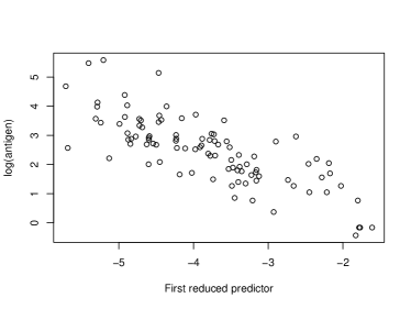
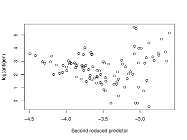
Figure 4: The scatter plots of $\log$(antigen) versus the first two reduced predictors

Fourier transform sparse inverse regression estimators for sufficient variable selection

This section discusses the Fourier transform sparse inverse regression estimators proposed by Weng (2022) in the high-dimensional regime, specifically when the sample size is smaller than the predictor dimension. It is often assumed that only a few predictors have a significant impact on the response variable. This implies the existence of a predictor subset, denoted by $S\in[p]$, such that

$$\mathbf{Y}\mathchoice{\mathrel{\hbox to0.0pt{$\displaystyle\perp$\hss}\mkern 2.0mu{\displaystyle\perp}}}{\mathrel{\hbox to0.0pt{$\textstyle\perp$\hss}\mkern 2.0mu{\textstyle\perp}}}{\mathrel{\hbox to0.0pt{$\scriptstyle\perp$\hss}\mkern 2.0mu{\scriptstyle\perp}}}{\mathrel{\hbox to0.0pt{$\scriptscriptstyle\perp$\hss}\mkern 2.0mu{\scriptscriptstyle\perp}}}\mathbf{X}\mid X_{S}.$$

Equivalently, there exists a representation of $\boldsymbol{\Gamma}$ such that its nonzero rows are located at the indices in the set $S$. We consider a quadratic discrepancy function of $\boldsymbol{\Gamma}\in\mathbb{R}^{p\times d}$ and $\mathbf{C}\in\mathbb{R}^{d\times 2k}$,

$$\begin{array}[]{cll}F(\boldsymbol{\Gamma},\mathbf{C})&=&[\text{vec}(\hat{\boldsymbol{\xi}})-\text{vec}(\boldsymbol{\Gamma}\mathbf{C})]^{T}\text{diag}\{\hat{\boldsymbol{\Sigma}}\}[\text{vec}(\hat{\boldsymbol{\xi}})-\text{vec}(\boldsymbol{\Gamma}\mathbf{C})]\\ &=&\left\|\hat{\boldsymbol{\Sigma}}^{1/2}\hat{\boldsymbol{\xi}}-\hat{\boldsymbol{\Sigma}}^{1/2}\boldsymbol{\Gamma}C\right\|_{F}^{2},\end{array}$$ (38)

where $\|\mathbf{A}\|_{F}$ is the Frobenius norm of matrix $\mathbf{A}$ defined by $\sqrt{\text{trace}(\mathbf{A}\mathbf{A}^{T})}$, and $\text{trace}(\cdot)$ denotes the trace of a matrix. Sufficient variable selection aims to identify the indexes of active predictors $S=\{1\leq j\leq p:\boldsymbol{e}_{j}^{T}\boldsymbol{\Gamma}\boldsymbol{\Gamma}^{T}\boldsymbol{e}_{j}>0\}$. To achieve both sufficient dimension reduction and sufficient variable selection simultaneously, Weng (2022) employed the coordinate-independent penalization (Chen et al., 2010), denoted as $p_{\boldsymbol{w}}(\boldsymbol{\Gamma})=\sum^{p}_{j=1}w_{j}\|\boldsymbol{e}_{i}^{T}\boldsymbol{\Gamma}\|_{2}$, where $\boldsymbol{w}=(w_{1},\cdots,w_{p})$ is the penalty weights. The objective function of interest is the quadratic function (38) equipped with the coordinate-independent penalty $p_{\boldsymbol{w}}(\boldsymbol{\Gamma})$ and a tuning parameter $\lambda$. The optimization problem is as follows

$$\begin{array}[]{ll}\hat{\boldsymbol{\Gamma}}=&\arg\min_{\boldsymbol{\Gamma},\mathbf{C}}\left\{\frac{1}{2}\left\|\hat{\boldsymbol{\Sigma}}^{1/2}\hat{\boldsymbol{\xi}}-\hat{\boldsymbol{\Sigma}}^{1/2}\boldsymbol{\Gamma}\mathbf{C}\right\|_{F}^{2}+\lambda p_{\boldsymbol{w}}(\boldsymbol{\Gamma})\right\},~{}~{}~{}~{}~{}~{}~{}\text{subject to}\ \mathbf{C}\mathbf{C}^{T}=\mathbf{I}_{d}.\end{array}$$ (39)

Given $\mathbf{C}$, this problem is convex with respect to $\boldsymbol{\Gamma}$. The nonsmooth penalty term $p_{\boldsymbol{w}}(\boldsymbol{\Gamma})$ encourages sparsity by shrinking small values of the rows in $\boldsymbol{\Gamma}$ towards zeros. The regularization parameter $\lambda$ controls model complexity.

Algorithm for sparse estimators

To solve the optimization problem (39), Weng (2022) considered an iterated alternating direction method of multipliers (ADMM) algorithm (Boyd et al., 2011). When solving for $\boldsymbol{\Gamma}$ given a specific $\mathbf{C}$ value, the following equivalent optimization problem is considered

$$\begin{array}[]{cll}&\arg\min_{\boldsymbol{\Gamma}}&\frac{1}{2}\left\|\hat{\boldsymbol{\Sigma}}^{1/2}\hat{\boldsymbol{\xi}}-\hat{\boldsymbol{\Sigma}}^{1/2}\boldsymbol{\Gamma}\mathbf{C}\right\|_{F}^{2}+\sum_{j=1}^{p}\lambda_{j}\left\|\mathbf{A}_{j\cdot}\right\|_{2},~{}~{}~{}~{}~{}~{}~{}~{}~{}~{}~{}~{}\mbox{subject to }\boldsymbol{\Gamma}-\mathbf{A}=\mathbf{0},\\ \end{array}$$ (40)

where $\lambda_{j}=\lambda w_{j}$ is the weight for each row of $\mathbf{A}$, i.e., $\mathbf{A}_{j\cdot}$. According to Boyd et al. (2011), the augmented Lagrangian function over $\boldsymbol{\Gamma}$, with the copy variable $\mathbf{A}$ and the scaled dual variable $\mathbf{U}$, is defined as

$$\begin{array}[]{cll}L_{\rho}(\boldsymbol{\Gamma},\mathbf{A},\mathbf{U})&:=&\frac{1}{2}\left\|\hat{\boldsymbol{\Sigma}}^{1/2}\hat{\boldsymbol{\xi}}-\hat{\boldsymbol{\Sigma}}^{1/2}\boldsymbol{\Gamma}\mathbf{C}\right\|_{F}^{2}+\sum_{j=1}^{p}\lambda_{j}\left\|\mathbf{A}_{j\cdot}\right\|_{2}+\frac{\rho}{2}\left\|\boldsymbol{\Gamma}-\mathbf{A}+\mathbf{U}\right\|_{F}^{2},\end{array}$$ (41)

where $\rho>0$ is the algorithm tuning parameter. Let $\boldsymbol{\Xi}=\boldsymbol{\Sigma}\boldsymbol{\xi}$ and $\hat{\boldsymbol{\Xi}}=\hat{\boldsymbol{\Sigma}}\hat{\boldsymbol{\xi}}$.

To minimize Equation (41) over $(\boldsymbol{\Gamma},\mathbf{A},\mathbf{U})$, we iterate the following three steps:

$$\boldsymbol{\Gamma}^{k+1} =\mathop{\rm arg\,min}_{\boldsymbol{\Gamma}}L_{\rho}(\boldsymbol{\Gamma},\mathbf{A}^{k},\mathbf{U}^{k}),$$ (42)

$$\mathbf{A}^{k+1} =\mathop{\rm arg\,min}_{\mathbf{A}}L_{\rho}(\boldsymbol{\Gamma}^{k+1},\mathbf{A},\mathbf{U}^{k}),$$ (43)

$$\mathbf{U}^{k+1} =\mathbf{U}^{k}+\boldsymbol{\Gamma}^{k+1}-\mathbf{A}^{k+1},$$ (44)

where $(\boldsymbol{\Gamma}^{k},\mathbf{A}^{k},\mathbf{U}^{k})$ denotes the $k^{th}$ iteration. The explicit solutions corresponding to each step are stated in Algorithm 7.

1. Update $\boldsymbol{\Gamma}^{k+1}=(\hat{\boldsymbol{\Sigma}}+\rho\mathbf{I}_{p})^{-1}(\hat{\boldsymbol{\Xi}}\mathbf{C}^{T}+\rho\mathbf{A}^{k}-\rho\mathbf{U}^{k})$.

2. Update $\mathbf{A}^{k+1}_{j\cdot}=\max\left\{1-\frac{\lambda_{j}/\rho}{\left\|\boldsymbol{\Gamma}_{j\cdot}^{k+1}+\mathbf{U}_{j\cdot}^{k}\right\|_{2}},0\right\}(\boldsymbol{\Gamma}_{j\cdot}^{k+1}+\mathbf{U}_{j\cdot}^{k})$ for $j=1,\cdots,p,$ and $\lambda_{j}=\lambda w_{j}$.

3. Update $\mathbf{U}^{k+1}=\mathbf{U}^{k}+\boldsymbol{\Gamma}^{k+1}-\mathbf{A}^{k+1}$.

4. Repeat steps 1-3 until $\left\|\boldsymbol{\Gamma}^{k+1}-\mathbf{A}^{k+1}\right\|_{F}<\epsilon$ and $\left\|\rho(\mathbf{A}^{k}-\mathbf{A}^{k+1})\right\|_{F}<\epsilon.$

Algorithm 7 Updating $\boldsymbol{\Gamma}$ given $\mathbf{C}$

Given $\boldsymbol{\Gamma}$ from Algorithm 7, we further update $\mathbf{C}$ based on the following optimization problem because the regularization term does not involve $\mathbf{C}$:

$$\begin{array}[]{rl}&{\arg\min}_{\mathbf{C}}\|\hat{\boldsymbol{\Sigma}}^{1/2}\hat{\boldsymbol{\xi}}-\hat{\boldsymbol{\Sigma}}^{1/2}\boldsymbol{\Gamma}\mathbf{C}\|_{F}^{2},~{}~{}~{}~{}~{}~{}~{}~{}\ \text{subject to}\ \boldsymbol{C}\mathbf{C}^{T}=\mathbf{I}_{d}.\\ \end{array}$$

The solution has a closed-form expression, that is $\hat{\mathbf{C}}=\mathbf{W}_{2}\mathbf{W}_{1}^{T},$ where $\mathbf{W}_{1}\mathbf{D}\mathbf{W}^{T}_{2}$ is the singular value decomposition of $\hat{\boldsymbol{\Xi}}^{T}\boldsymbol{\Gamma}$. Let $L(\boldsymbol{\Gamma},\mathbf{C})=\frac{1}{2}\left\|\hat{\boldsymbol{\Sigma}}^{1/2}\hat{\boldsymbol{\xi}}-\hat{\boldsymbol{\Sigma}}^{1/2}\boldsymbol{\Gamma}\mathbf{C}\right\|_{F}^{2}+\lambda p_{\mathbf{w}}(\boldsymbol{\Gamma})$.

1. Initialize the algorithm with $\boldsymbol{\Gamma}^{0}$ and equal weight $\boldsymbol{w}^{0}$. Start with $j=0$.

2. Update $\boldsymbol{C}^{j+1}=\boldsymbol{W}_{2}\boldsymbol{W}_{1}^{T}$, where $\boldsymbol{W}_{1}\boldsymbol{D}\boldsymbol{W}^{T}_{2}$ = SVD($\widehat{\boldsymbol{\Xi}}^{T}\boldsymbol{\Gamma}^{j}$) and $\boldsymbol{\Gamma}^{j+1}$ using Algorithm 7 with input $\boldsymbol{C}^{j+1}$.

3. Repeat step 2 with $j=j+1$ or stop if $|L(\boldsymbol{\Gamma}^{j+1},\boldsymbol{C}^{j+1})-L(\boldsymbol{\Gamma}^{j},\boldsymbol{C}^{j})|<\epsilon.$

4. Update weights $\mathbf{w}_{i}=\frac{1}{\left\|\mathbf{e}^{T}_{i}\boldsymbol{\Gamma}\right\|_{2}^{1/2}}$ for $i=1,\cdots,p.$

5. Finally, repeat steps 2-3 using the new weights.

Algorithm 8 Iterated ADMM

Algorithm 8 starts with equal weights $\mathbf{w}^{0}$, i.e., $(1,\cdots,1)^{T}$, and then updates weights using $\boldsymbol{\Gamma}$ values. It is sufficient to update weights once to avoid overshrinkage of the estimation.

R functions for Fourier transform sparse inverse regression estimators

In this section, we describe the admmft() function available in itdr package, which enables the selection of active variables using the Fourier transformation method (Weng, 2022). The following R codes demonstrate the application of this function for sufficient variable selection on the Raman dataset in itdr package. By default, the tuning parameter $\lambda$ is set to $0.5$. However, if no specific value is provided, the function utilizes cross-validation to determine the optimal lambda value.

    data(raman)    Y=as.matrix(Raman[,c(1100)]) ## percentage of total fat content    X=as.matrix(Raman[c(2:501)]) ## first 500 wavelength variables    out = admmft(X,Y,d = 1, m = 30, lambda = 0.5, sparse.cov=T, scale.X=T)    estbeta = out$B    plot(Y ~ X %*% estbeta, xlab = "First reduced predictor",    ylab = "Percentage of total fat")The admmft() function accepts the following arguments: $\mathbf{X}$, the predictor matrix of dimension $n\times p$; $\mathbf{Y}$, the response matrix of dimension $n\times q$; $d$, the dimension of the central subspace; $m$, the number of Fourier transforms used in constructing the kernel matrix; lambda, the tuning parameter. If it is not provided, then the optimal lambda value is chosen by cross-validation using the Fourier transformation method; noB, the number of iterations for updating B, the default value is $5$; noC, the number of iterations for updating C, the default value is $20$; noW, the number of iterations for updating the weight, the default value is $2$; sparse.cov, a logical value that determines whether to calculate the soft-threshold matrix for the covariance matrix. If set to TRUE, the soft-threshold matrix is computed. scale.X, a logical value that determines whether to standardize each variable when calculating the soft-threshold matrix for the covariance matrix. If set to TRUE, variables are standardized.

Based on the results shown in Figure 5, it can be inferred that the first direction obtained from the ADMM Fourier transformation approach exhibits a discernible downward trend in relation to the percentage of total fat content.

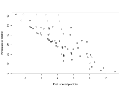
Figure 5: The scatter plot of $\log$(antigen) versus the first two reduced predictors

Summary

This paper has introduced the $\mathbf{itdr}$ R package which offers a comprehensive set of functions for estimating the central subspace (CS) and the central mean subspace (CMS) using integral transformation methods. We have provided an overview of the sufficient dimension reduction technique and discussed various integral transformation methods, including the Fourier transformation method, the convolution transformation method, the iterative Hessian transformation method, the Fourier transformation approach for inverse regression, the minimum discrepancy approach, and Fourier transform sparse inverse regression. The first three methods are specifically designed for univariate responses, whereas the latter three methods are applicable to both univariate and multivariate responses. The $\mathbf{itdr}$ package equips users with powerful tools to estimate the dimension and sufficient dimension reduction subspaces. Additionally, it provides essential functions and options to relax the normality assumption through the estimation of the density function using the kernel smoothing method. These features expand the potential applications of the package to a wider range of domains.

Tharindu P. De Alwis
School of Mathematical and Statistical Sciences,
Southern Illinois University Carbondale
1245 Lincoln Drive,
Carbodnale, IL-62901
United States
(0000-0002-3446-0502)
mktharindu87@siu.edu

S. Yaser Samadi
School of Mathematical and Statistical Sciences,
Southern Illisnois University Carbondale
1245 Lincoln Drive,
Carbodnale, IL-62901
United States
(0000-0002-6121-0234)
ysamadi@siu.edu

Jiaying Weng
Department of Mathematical Sciences,
Bentley University
175 Forest Street,
Waltham, MA-02452
United States
(0000-0002-9463-5714)
jweng@bentley.edu

References

- Adragni and Raim (2014) K. P. Adragni and A. M. Raim. ldr: An r software package for likelihood-based sufficient dimension reduction. Journal of Statistical Software, 61:1–21, 2014.
- Bentler and Xie (2000) P. M. Bentler and J. Xie. Corrections to test statistics in principal hessian directions. Statistics and Probability Letters, 47:381–389, 2000.
- Boyd et al. (2011) S. Boyd, N. Parikh, E. Chu, B. Peleato, J. Eckstein, et al. Distributed optimization and statistical learning via the alternating direction method of multipliers. Foundations and Trends® in Machine learning, 3(1):1–122, 2011.
- Chen et al. (2010) X. Chen, C. Zou, and R. D. Cook. Coordinate-independent sparse sufficient dimension reduction and variable selection. Annals of Statistics, 38(6):3696–3723, 2010.
- Clark et al. (1987) R. G. Clark, H. V. Henderson, G. K. Hoggard, R. S. Ellison, and B. J. Young. The ability of biochemical and haematological tests to predict recovery in periparturient recumbent cows. NZ Veterinary Journal, 35:126–133, 1987.
- Cook (1998) R. D. Cook. Regression Graphics: Ideas for Studying Regressions Through Graphics. New York: Wiley, 1998.
- Cook (2007) R. D. Cook. Fisher Lecture: Dimension Reduction in Regression. Statistical Science, 22(1):1 – 26, 2007.
- Cook and Forzani (2008a) R. D. Cook and L. Forzani. Covariance reducing models: An alternative to spectral modeling of covariance matrices. Biometrika, 95(4):799–812, 2008a.
- Cook and Forzani (2008b) R. D. Cook and L. Forzani. Principal fitted components for dimension reduction in regression. Statistical Science, 23(4):485–501, 2008b.
- Cook and Forzani (2009) R. D. Cook and L. Forzani. Likelihood-based sufficient dimension reduction. Journal of the American Statistical Association, 104:197–208, 2009.
- Cook and Li (2002) R. D. Cook and B. Li. Dimension reduction for the conditional mean in regression. Annals of Statistics, 30:455–474, 2002.
- Cook and Ni (2005) R. D. Cook and L. Ni. Sufficient dimension reduction via inverse regression: A minimum discrepancy approach. Journal of the American Statistical Association, 100:410–428, 2005.
- Cook and Weisberg (1991) R. D. Cook and S. Weisberg. Sliced inverse regression for dimension reduction: Comment. Journal of the American Statistical Association, 86:328–332, 1991.
- Feng et al. (2013) Z. Feng, M. X. Wen, Z. Yu, and L. Zhu. On partial sufficient dimension reduction with applications to partially linear multi-index models. Journal of the American Statistical Association, 108:236–246, 2013.
- Folland (1992) G. B. Folland. Fourier Analysis and its Applications. Brooks/Cole, 1992.
- Hang and Xia (2019) W. Hang and Y. Xia. MAVE: Methods for Dimension Reduction. The Comprehensive R Archive Network, 2019. URL https://CRAN.R-project.org/package=MAVE.
- Hristache et al. (2001) M. Hristache, A. Juditsky, J. Polzehl, and V. G. Spokoiny. Structure adaptive approach for dimension reduction. Annals of Statistics, 29:1537–1566, 2001.
- Li (2018) B. Li. Sufficient dimension reduction: Methods and applications with R. CRC Press, Boca Raton, FL, 2018.
- Li and Kim (2021) B. Li and K. Kim. nsdr: Nonlinear Sufficient Dimension Reduction. The Comprehensive R Archive Network, 2021. URL https://CRAN.R-project.org/package=nsdr.
- Li (1991) K. C. Li. Sliced inverse regression for dimension reduction. Journal of the American Statistical Association, 86(414):316–327, 1991.
- Li (1992) K. C. Li. On principal hessian directions for data visualization and dimension reduction: Another application of stein’s lemma. Journal of the American Statistical Association, 87:1025–1039, 1992.
- Ma and Zhu (2013) Y. Ma and L. Zhu. Efficient estimation in sufficient dimension reduction. Annals of Statistics, 41:250–268, 2013.
- Weisberg (2015) S. Weisberg. dr: Methods for Dimension Reduction for Regression. The Comprehensive R Archive Network, 2015. URL https://CRAN.R-project.org/package=dr.
- Weng (2022) J. Weng. Fourier transform sparse inverse regression estimators for sufficient variable selection. Computational Statistics & Data Analysis, 168:107380, 2022.
- Weng and Yin (2018) J. Weng and X. Yin. Fourier transform approach for inverse dimension reduction method. Journal of Nonparametric Statistics, 30(4):1049–1071, 2018.
- Weng and Yin (2022) J. Weng and X. Yin. A minimum discrepancy approach with fourier transform in sufficient dimension reduction. Statistica Sinica, 32:2381–2403, 2022.
- Xia et al. (2002) Y. Xia, H. Tong, W. Li, and L. X. Zhu. An adaptive estimation of dimension reduction. Journal of the Royal Statistical Society. Series B, 64:363–410, 2002.
- Zeng and Zhu (2010) P. Zeng and Y. Zhu. An integral transform method for estimating the central mean and central subspaces. Journal of Multivariate Analysis, 101(1):271–290, 2010.
- Zhu et al. (2019) R. Zhu, J. Zhang, R. Zhao, PengXu, W. Zhou, and XinZhang. orthodr: Semiparametric dimension reduction via orthogonality constrained optimization. The R Journal, 11:24–37, 2019.
- Zhu and Zeng (2006) Y. Zhu and P. Zeng. Fourier methods for estimating the central subspace and the central mean subspace in regression. Journal of the American Statistical Association, 101:1638–1651, 2006.