Type III seesaw under $A_{4}$ modular symmetry with leptogenesis

Abstract

We make an attempt to study neutrino phenomenology in the framework of type-III seesaw by considering $A_{4}$ modular symmetry in the super-symmetric context. In addition, we have included a local $U(1)_{B-L}$ symmetry which eventually helps us to avoid certain unwanted terms in the superpotential. Hitherto, the seesaw being type-III, it involves three fermion triplet superfields $\Sigma_{R}$, along with which, we have included a singlet weighton field $(\rho)$. In here, modular symmetry plays a crucial role by avoiding the usage of excess flavon (weighton) fields. Also, the Yukawa couplings acquire modular forms which are expressed in terms of Dedekind eta function $\eta(\tau)$. However, for numerical analysis we use $q$ expansion expressions of these couplings. Therefore, the model discussed here is triumphant enough to accommodate the observed neutrino oscillation data and also successfully explains observed baryon asymmetry of the universe through leptogenesis.

I INTRODUCTION

Decades ago when standard model (SM) was built it seemed impeccable, but its foundation was again questioned when some unresolved puzzles came into existence. To name a few, it does not provide any satisfactory explanation to the tininess of neutrino mass Ma:1998dn , neutrino oscillation, strong CP problem, matter-antimatter asymmetry, the nature of dark matter and dark energy, etc. To resolve the issue regarding smallness of neutrino masses within the context of SM, Weinberg operator (Weinberg:1979sa, ; Abada:2007ux, ) helps to an extent. However, to demonstrate other phenomena, we need to go beyond standard model (BSM), so introducing right handed (RH) neutrinos becomes a necessity. This becomes the basis of canonical seesaw mechanism, i.e., as soon as these RH neutrinos come into picture, they allow Dirac mass terms for neutrinos. In this regard, type-I seesaw (Minkowski:1977sc, ; Yanagida:1979as, ; Glashow:1979nm, ; Mohapatra:1979ia, ) is the simplest one, which includes singlet heavy ($\simeq 10^{14}$ GeV) RH neutrinos and brings down the mass scale of active neutrinos to $0.1$ eV range, as observed from experimental data. Also, there exists other variants of seesaw i.e., type-II Mohapatra:1980yp ; Antusch:2004xy ; Gu:2006wj ; Arhrib:2011uy ; Ghosh:2017pxl which incorporates scalar triplets, type-III Foot:1988aq ; Liao:2009nq involving fermion triplets, linear seesaw Ma:2009du ; Wang:2015saa ; Borah:2018nvu ; CarcamoHernandez:2020pnh ; Sruthilaya:2017mzt and inverse seesaw Hirsch:2009mx ; Gu:2010xc ; Das:2012ze ; Arganda:2014dta ; Dias:2012xp ; Dev:2012sg ; Dias:2011sq ; Bazzocchi:2010dt which are modified type-I seesaw. In this work, we intend to study the case of type-III seesaw in the context of discrete $A_{4}$ modular symmetry as it has not been studied earlier in this framework. In general, it is presumed that type III seesaw is more complicated compared to the canonical type I seesaw due to the involvement of triplet fermions. However, it has been shown in Refs. Barr:2003nn ; Albright:2003xb that, in some cases, e.g., realistic $SO(10)$ model, type III seesaw may have less difficulty in reproducing realistic neutrino masses and mixings than the conventional type-I seesaw. Therefore, in this work we would like to investigate the implications of $A_{4}$ modular symmetry in the context of type III seesaw for describing the observed neutrino oscillation data.

It is interesting to notice that many non-abelian discrete symmetries i.e., $S_{3}$ (Ma:2004zd, ; Kubo:2003iw, ; Pakvasa:1977in, ; Ma:2014qra, ), $A_{4}$ (Ma:2001dn, ; Babu:2002dz, ; Altarelli:2005yp, ; Ma:2004zv, ), $S_{4}$ (Ma:2005pd, ; Krishnan:2012me, ; Grimus:2009pg, ) etc. and continuous symmetries like $U(1)_{B-L}$ (Mishra:2020fhy, ; Ma:2015raa, ; Singirala:2017see, ; Singirala:2017cch, ; Nomura:2017jxb, ; Nomura:2017vzp, ; Nomura:2017kih, ), $U(1)_{L_{e}-L_{\mu}}$ (Behera:2021nuk, ; Foot:1990mn, ; Panda:2022kbn, ; He:1991qd, ), $U(1)_{H}$ (Nardi:2000px, ; Ibanez:1994ig, ; Binetruy:1994ru, ; Nir:1995bu, ) etc. come to our rescue to develop the model and generate neutrino mass matrix, which gives results in-accordance with experimental data. Implementation of the discrete non-abelian symmetries demand the usage of excess flavon fields. These flavon insertions make the Yukawa interaction terms non-renormalizable and bring down the predictability of the model. Therefore, a clever approach of modular symmetry (Ferrara:1989bc, ; Ferrara:1989qb, ; Leontaris:1997vw, ; feruglio2019neutrino, ; King:2020qaj, ) is introduced to breach the scenario of flavon fields. In here, the approach involves discrete symmetry group because they are isomorphic to finite modular groups, for example, $\Gamma_{2}\simeq S_{3}$ (Okada:2019xqk, ; Kobayashi:2018vbk, ; Kobayashi:2018wkl, ; Kobayashi:2019rzp, ), $\Gamma_{3}\simeq A_{4}$ (Behera:2020lpd, ; Nomura:2022boj, ; Kashav:2022kpk, ; Kashav:2021zir, ; Behera:2020sfe, ; Asaka:2020tmo, ; Abbas:2020vuy, ; Okada:2020dmb, ; Altarelli:2005yx, ), $\Gamma_{4}\simeq S_{4}$ (Kobayashi:2019xvz, ; Wang:2019ovr, ; Okada:2019lzv, ; King:2019vhv, ; Kobayashi:2019mna, ; Novichkov:2018ovf, ; Penedo:2018nmg, ), $\Gamma_{5}\simeq A_{5}$ Criado:2019tzk ; Novichkov:2018nkm ; Ding:2019xna , $\Gamma^{\prime}_{5}\simeq A^{\prime}_{5}$ (Behera:2021eut, ; Behera:2022wco, ; Yao:2020zml, ; Wang:2020lxk, ) etc. We make an attempt to use $A_{4}$ modular symmetry, which is isomorphic to $\Gamma_{3}$. The alluring feature of modular symmetry is that, it transforms Yukawa couplings i.e., it makes them modular in nature. Therefore, the flexibility to fine tune the Yukawa couplings is lost and now it is governed by the modulus $\tau$. The involvement of modulus $\tau$ is seen in the expression of Dedekind eta function, as shown in eqn.(55), and further the acquisition of VEV by it, helps in the symmetry breaking of the $A_{4}$ group. As, $N=3$ for $\Gamma_{3}\simeq A_{4}$ is finite, hence, they can be constructed using $k=1$ being the lowest weight. The dimension of $\Gamma_{3}$ being $2k+1$ (see appendix D of feruglio2019neutrino ) yielding three linearly independent $Y_{i}(\tau)$ shown in eqns. (52 $-$ 54). These Yukawa couplings are utilised in curating the neutrino mass matrices after applying the $A_{4}$ product rules and are implicitly governed by the range of modulus $\tau$, as will become more clear while performing the analysis numerically. Further, we are able to explain the baryon asymmetry of the universe through leptogenesis (Davidson:2008bu, ; Fukugita:1986hr, ), because of presence of heavy RH neutrino, which yields the order of lepton asymmetry to be $\sim 10^{-10}$.

This work is organised as follows. In Sec.II, we discuss the model framework containing particles contributing towards expressing the superpotential for type-III seesaw and its associated mass matrices. Further, in Sec.III, we perform the numerical analysis where a common parameter space along with best-fit data set are extracted using chi-square minimization technique using the data of all the phenomena discussed in our model. Additionally, Sec.IV sheds light on lepton asymmetry generated through leptogenesis, in the context of our model and collider bound on the mass of new gauge boson $Z^{\prime}$ is presented in Sec. V. Finally, in Sec. VI, we conclude our results.

II Model Framework

In order to fulfil our desired goal, we incorporate new particles and assign them suitable charges under extended symmetries (i.e., modular $A_{4}$ and $U(1)_{B-L}$), as presented in Table-1, such that the superpotential remains invariant. The idea behind the inclusion of $U(1)_{B-L}$ symmetry along with $A_{4}$ modular symmetry is to avoid certain unwanted terms in the superpotential which is not possible by $A_{4}$ modular symmetry. The suitability to go beyond standard model (BSM) paves the way to include heavy RH neutrinos $\Sigma_{R}$ in our model, which transform as triplet under $SU(2)_{L}$, and accompanying these, we have also included a weighton ($\rho$). These symmetries are broken at a very high scale, much greater than the scale of electroweak symmetry breaking. The $U(1)_{B-L}$ symmetry is spontaneously broken by assigning non-zero VEV to the singlet weighton $\rho$ and the $Z^{\prime}$ boson associated with it acquires its mass by the singlet VEV $v_{\rho}$. We will show in sec.V that its mass and gauge coupling satisfy the present experimental bounds. Moreover, the non-zero VEV acquired by the singlet weighton helps heavy RH neutrinos to gain mass. We implement modular symmetry because it restricts the usage of excess flavon fields, which otherwise, overfill the particle gamut and reduces the predictability of the model while working in BSM. This becomes possible only because Yukawa couplings acquire modular form and also takeover the job performed by extra flavon fields. In addition, the complete superpotential of our model is represented below,

Fields	$E^{c}_{R_{1}}$	$E^{c}_{R_{2}}$	$E^{c}_{R_{3}}$	$L$	$\Sigma^{c}_{Ri}$	$H_{u,d}$	$\rho$
$SU(2)_{L}$	$1$	$1$	$1$	$2$	$3$	$2$	$1$
$U(1)_{Y}$	$1$	$1$	$1$	$-\frac{1}{2}$	$0$	$\frac{1}{2}$,$-\frac{1}{2}$	$0$
$U(1)_{B-L}$	$1$	$1$	$1$	$-1$	$1$	$0$	$-2$
$A_{4}$	$1$	$1^{\prime}$	$1^{\prime\prime}$	$1,1^{\prime\prime},1^{\prime}$	$3$	$1$	$1$
$k_{I}$	$0$	$0$	$0$	$0$	$-2$	$0$	$2$

Table 1: Particle content of the model and their charges under ${SU(2)_{L}\times U(1)_{Y}\times U(1)_{B-L}}\times A_{4}$, where, $k_{I}$ is the modular weight.

Yukawa couplings	$A_{4}$	$k_{I}$
$Y=(y_{1},y_{2},y_{3})$	$3$	$2$

Table 2: Charge assignment to Yukawa coupling under $A_{4}$ and its modular weight.

$$\mathcal{W}_{III} =\mathcal{W}_{M_{\ell}}+\mathcal{W}_{M_{D}}+\mathcal{W}_{M_{R}},$$ (1)

where, the terms $\mathcal{W}_{M_{\ell}}$, $\mathcal{W}_{M_{D}}$ and $\mathcal{W}_{M_{R}}$ are responsible for generating the mass term for the charged leptons, Dirac mass term for the neutrinos and Majorana mass term for the RH neutrinos and their explicit forms are provided in the following subsections.
Masses of charged leptons

We urge to have a simplified form of charged lepton mass matrix for which we assign $U(1)_{B-L}$ charge to the right-handed (RH) charged leptons i.e., $E_{Ri}^{c}$ as $+1$, and three generations of left-handed (LH) charged leptons have the value $-1$. While under $A_{4}$ symmetry RH and LH charged leptons transform as $\{1,1^{\prime},1^{\prime\prime}\}$ and {$1,1^{\prime\prime},1^{\prime}$}. In addition, the modular weight assigned to the charged leptons is zero. The Higgsinos $H_{u,d}$ are given charges $0$ and $1$ under $U(1)_{B-L}$ and $A_{4}$ symmetry respectively, with zero modular weight. The VEVs of Higgsinos i.e., $(v_{u},v_{d})$ are related to the SM Higgs VEV $(v_{H})$ by a simple equation $v_{H}=\frac{1}{2}\sqrt{v_{u}^{2}+v_{d}^{2}}$. The ratio of Higgsinos VEV is written as $\tan\beta=({v_{u}}/{v_{d}})\simeq 5$ (used in our analysis) Antusch:2013jca ; Okada:2019uoy ; Bjorkeroth:2015ora . The admissible superpotential term for the charged lepton sector is given below:

$$\mathcal{W}_{M_{\ell}} =y_{ij}E^{c}_{R_{i}}H_{d}L_{j}\;.$$ (2)

After the electroweak symmetry breaking the mass matrix for the charged leptons takes the diagonal form:

$$M_{\ell} =\frac{v_{d}}{\sqrt{2}}\left[\begin{array}[]{ccc}y_{ee}&0&0\\ 0&y_{\mu\mu}&0\\ 0&0&y_{\tau\tau}\\ \end{array}\right].$$ (6)

Dirac mass term

The neutral lepton sector gets mass as and when $H_{u}$ acquires non-vanishing VEV. To keep Dirac term invariant under $A_{4}$ modular group, we need fermion triplets to have charge $3$ as Yukawa couplings are triplet (Y=$(y_{1},y_{2},y_{3}$)). Hence, the Dirac interaction term of neutral multiplet of fermion triplet with the SM left-handed neutral leptons can be written as:

$$\mathcal{W}_{M_{D}} =-~{}(G_{D})_{ij}\left[{H_{u}}\Sigma^{c}_{R_{i}}\sqrt{2}\textbf{Y}L_{j}\right]\;,$$ (7)

with $G_{D}$= diag{$\alpha_{1},\alpha_{2},\alpha_{3}$}, which gives the mass matrix

$$M_{D} =v_{u}\left[\begin{array}[]{ccc}\alpha_{1}&0&0\\ 0&\alpha_{2}&0\\ 0&0&\alpha_{3}\\ \end{array}\right]\left[\begin{array}[]{ccc}y_{1}&y_{3}&y_{2}\\ y_{2}&y_{1}&y_{3}\\ y_{3}&y_{2}&y_{1}\\ \end{array}\right].$$ (14)

Majorana mass term

The superpotential for Majorana mass term for right handed neutrinos is given as,

$$\mathcal{W}_{M_{R}}=-\frac{M^{\prime}_{\Sigma}}{2}\left(\beta_{\Sigma}{\rm{Tr}}\left[\mathbf{{\Sigma^{c}_{R_{i}}}}\textbf{Y}\mathbf{{\Sigma^{c}_{R_{i}}}}\right]_{\rm{sym}}+\gamma_{\Sigma}{\rm{Tr}}\left[\mathbf{{\Sigma^{c}_{R_{i}}}}\textbf{Y}\mathbf{{\Sigma^{c}_{R_{i}}}}\right]_{\rm asym}\right)\frac{\rho}{\Lambda}\;,$$ (15)

where, $M^{\prime}_{\Sigma}$ is the free mass parameter and $\Sigma^{c}_{R_{i}}$ with $(i=1,2,3)$, which can be represented in $SU(2)$ basis as,

$$\Sigma^{c}_{R_{i}}=\begin{pmatrix}\Sigma^{0~{}c}_{R_{i}}/\sqrt{2}~{}&~{}\Sigma^{-~{}c}_{R_{i}}\\ \Sigma^{+~{}c}_{R_{i}}~{}&~{}-\Sigma^{0~{}c}_{R_{i}}/\sqrt{2}\end{pmatrix}.$$ (16)

Applying $A_{4}$ symmetry product rule to eqn. (15), yields both symmetric and anti-symmetric parts with $\beta_{\Sigma}$ = diag{$\beta_{1},\beta_{2},\beta_{3}$} and $\gamma_{\Sigma}$ = diag{$\gamma_{1},\gamma_{2},\gamma_{3}$} being the associated free parameter matrices respectively:

$$M_{R} =\frac{v_{\rho}}{\Lambda\sqrt{2}}\left(\frac{M^{\prime}_{\Sigma}}{2}\right)\left(\frac{\beta_{\Sigma}}{3}\left[\begin{array}[]{ccc}2y_{1}&-y_{3}&-y_{2}\\ -y_{3}&2y_{2}&-y_{1}\\ -y_{2}&-y_{1}&2y_{3}\\ \end{array}\right]+\gamma_{\Sigma}\left[\begin{array}[]{ccc}0&y_{3}&-y_{2}\\ -y_{3}&0&y_{1}\\ y_{2}&-y_{1}&0\\ \end{array}\right]\right).$$ (23)

The active neutrino mass matrix in the framework of type-III seesaw is given as,

$$m_{\nu} =-M_{D}M_{R}^{-1}M_{D}^{T}\;.$$ (24)

III Numerical Analysis

The global fit neutrino oscillation data at 3$\sigma$ interval from Esteban:2020cvm is used for numerical analysis, as given in Table 3.

Oscillation Parameters	Best fit value $\pm$ $1\sigma$	2$\sigma$ range	3$\sigma$ range
$\Delta m^{2}_{21}[10^{-5}~{}{\rm eV}^{2}]$	7.56$\pm$0.19	7.20–7.95	7.05–8.14
$|\Delta m^{2}_{31}|[10^{-3}~{}{\rm eV}^{2}]$ (NO)	2.55$\pm$0.04	2.47–2.63	2.43–2.67
$\sin^{2}\theta_{12}/10^{-1}$	3.21${}^{+0.18}_{-0.16}$	2.89–3.59	2.73–3.79
$\sin^{2}\theta_{23}/10^{-1}$ (NO)	4.30${}^{+0.20}_{-0.18}$	3.98–4.78 & 5.60–6.17	3.84–6.35
	5.98${}^{+0.17}_{-0.15}$	4.09–4.42 & 5.61–6.27	3.89–4.88 & 5.22–6.41
$\sin^{2}\theta_{13}/10^{-2}$ (NO)	2.155${}^{+0.090}_{-0.075}$	$1.98-2.31$	$2.04-2.43$
$\delta_{CP}/\pi$ (NO)	1.08${}^{+0.13}_{-0.12}$	$0.84-1.42$	$0.71-1.99$

Table 3: The global-fit values of the oscillation parameters along with their 1$\sigma$/2$\sigma$/3$\sigma$ ranges.

The neutrino mass matrix calculated using eqn.(24) is numerically diagonalized using the relation $U^{\dagger}\mathcal{M}U={\rm diag}(m_{\nu_{1}}^{2},m_{\nu_{2}}^{2},m_{\nu_{3}}^{2})$, where, ${\cal M}=m_{\nu}m_{\nu}^{\dagger}$ and $U$ is a unitary matrix, from which the neutrino mixing angles can be derived using the conventional relations:

$$\sin^{2}\theta_{13}=|U_{13}|^{2},~{}~{}~{}~{}\sin^{2}\theta_{12}=\frac{|U_{12}|^{2}}{1-|U_{13}|^{2}}\;,~{}~{}~{}~{}~{}\sin^{2}\theta_{23}=\frac{|U_{23}|^{2}}{1-|U_{13}|^{2}}\;.$$ (25)

Other observables related to the mixing angles and phases of PMNS matrix are

$$J_{CP} = \text{Im}[U_{e1}U_{\mu 2}U_{e2}^{*}U_{\mu 1}^{*}]=s_{23}c_{23}s_{12}c_{12}s_{13}c^{2}_{13}\sin\delta_{CP}\;,$$ (26)

$$\langle m_{ee}\rangle = |m_{\nu_{1}}\cos^{2}\theta_{12}\cos^{2}\theta_{13}+m_{\nu_{2}}\sin^{2}\theta_{12}\cos^{2}\theta_{13}e^{i\alpha_{21}}+m_{\nu_{3}}\sin^{2}\theta_{13}e^{i(\alpha_{31}-2\delta_{CP})}|.$$ (27)

The effective Majorana mass parameter $\langle m_{ee}\rangle$ is expected to have improved sensitivity measured by KamLAND-Zen experiment in coming future KamLAND-Zen:2016pfg . Further, we chose the following model parameter ranges to fit the present neutrino oscillation data:

$${\rm Re}[\tau]\in[-0.5,0.5],~{}~{}{\rm Im}[\tau]\in[0.75,2],\quad M^{\prime}_{\Sigma}\in[10^{4},10^{5}]\ {\rm TeV},\quad v_{\rho}\in[10^{3},10^{4}]~{}{\rm TeV},$$

$$\Lambda\in[10^{4},10^{5}]\ {\rm TeV},~{}~{}G_{D}\in[10^{-8},{10^{-5}}],~{}~{}\beta_{\Sigma}\in[{10^{-5}},10^{-1}],~{}~{}\gamma_{\Sigma}\in[10^{-9},10^{-10}].$$ (28)

We consider the free mass parameter ($M^{\prime}_{\Sigma}$), real and imaginary part of $\tau$, VEV of weighton ($v_{\rho}$) and cut-off parameter ($\Lambda$) randomly in the range given in eqn.(28). The range of $\tau$ is taken to be $[-0.5,0.5]$ for the real part and $[0.75,2]$ for the imaginary part, which provides the validity of model to follow normal hierarchy (NH). Considering these ranges, we arbitrarily scrutinise the input values of parameters and extract the best-fit values of those by applying chi-square minimization technique. The approach followed here by considering the general chi-square formula Roe:2015fca ; Ding:2021eva , which is utilized for calculating the $\chi^{2}$ values for all the available observables of the neutrino sector, like two mass squared differences and three mixing angles, further yielding cumulative $\chi^{2}$ minimum allowing us to get the values of the free parameters corresponding to the minimum i.e., best-fit values Wang:2020lxk ; Novichkov:2020eep . As there are a large number of free parameters involved in this framework, i.e., total number of free parameters are much larger than the number of observed neutrino oscillation parameters, it is not possible to get a constrained a correlated plot. Therefore, we calculate minimal chi-square and the the associated values of free parameters are considered as the best-fit values of the free parameters. Hence, Table 4 is obtained by keeping the experimentally observed oscillation parameters along with the cosmological bound for sum of neutrino masses $\Sigma m_{\nu_{i}}\leq 0.12~{}\rm eV$ (Planck:2018vyg, ).

Model Parameters	$\alpha_{1}$	$\alpha_{2}$	$\alpha_{3}$	$\beta_{1}$	$\beta_{2}$	$\beta_{3}$
Best-fit values	$3.83\times 10^{-7}$	$1.61\times 10^{-6}$	$5.73\times 10^{-7}$	$4.44\times 10^{-2}$	$~{}~{}~{}~{}0.824~{}~{}~{}~{}$	$1.05\times 10^{-3}$

Table 4: Best-fit of model parameters by under constraint of experimentally observed data.

We have not mentioned the best-fit values of $\gamma_{\Sigma}$ here in the Table 4, since it gives negligible contribution to the observables as compared to $G_{D}$ and $\beta_{\Sigma}$, hence, conventionally we deal with total six free parameters. As a consequence, the left panel of Fig.1 projects the correlation between $\sin^{2}\theta_{13}$ w.r.t. $\sum m_{\nu_{i}}$, where, the sum of neutrino mass is above its lower bound i.e., $0.058$eV (RoyChoudhury:2019hls, ), while the right panel shows the inter-dependence of $\sum m_{\nu_{i}}$ with ($\sin^{2}\theta_{12},\sin^{2}\theta_{23}$) with grid-lines showing their respective $3\sigma$ ranges. Moreover, in Fig. 2 the left panel shows an interdependence of $\sin^{2}\theta_{13}$ with Jarlskog invariant $|J_{CP}|$ whose value is constrained to be $|J_{CP}|\leq 7.1\times 10^{-3}$. As can be seen in the plot of $\delta_{CP}$ against $\sin^{2}\theta_{13}$ on the right panel of Fig. 2, $\delta_{CP}$ is varying in the range $[202^{\circ}$ - $211^{\circ}]$ while constrained by 3$\sigma$ bound of $\sin^{2}\theta_{13}$.

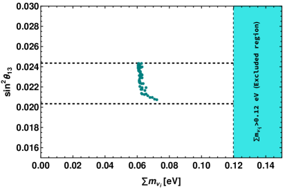
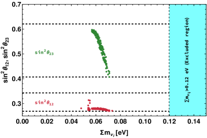
Figure 1: Left(right) panel shows the plane of the mixing angle i.e., $\sin^{2}\theta_{13}$ ($\sin^{2}\theta_{12},\sin^{2}\theta_{23}$) with sum of neutrino mass for the best fit values of model parameters while grid-lines represent the $3\sigma$ range of mixing angles.

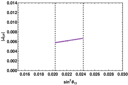
Figure 2: Left (right) panel shows the correlation of $\sin^{2}\theta_{13}$ with $J_{CP}$ ($\delta_{CP}$).

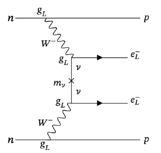
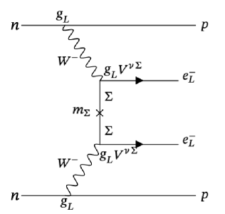
Figure 3: Feynman diagrams contributing to neutrinoless double beta decay with $W^{-}-W^{-}$ mediation via the exchange of virtual light neutrinos $\nu$ (left panel), and the exchange of virtual heavy neutrinos $\Sigma$ (right panel), where $g_{L}$ represents the SM weak coupling.

The process of neutrinoless double beta decay (NDBD) involves the simultaneous conversion of two neutrons into two protons and two electrons without any emission of neutrinos Nucciotti:2007jk ; Robertson:2013ziv ; Cardani:2018lje ; Dolinski:2019nrj , as shown in the left panel of Fig. 3. In the presence of new heavy neutral fermions, the additional contribution to the NDBD is linked to the mixing between active and heavy neutrinos and is expected to be rather small. The mixing of active and sterile neutrinos is generally descibed by the parameters $U_{\alpha i}$ and $\Theta_{\alpha i}$ which plays a crucial role Asaka:2011pb in the description of neutrinoless double beta decay. Thus, the $6\times 6$ neutrino mass matrix takes the form

$$\hat{M}=\begin{pmatrix}0&M_{D}\\ M_{D}^{T}&M_{\Sigma}\end{pmatrix}.$$ (29)

We can diagonalize it by using the unitary matrix $\hat{U}$ as $\hat{U}^{\dagger}\hat{M}\hat{U}^{*}=\hat{M}^{diag}$. The seesaw mechanism shows that $\hat{U}$ at the leading order takes the form Asaka:2011pb

$$\hat{U}=\begin{pmatrix}U&\Theta\\ -\Theta^{\dagger}U&1\end{pmatrix},$$ (30)

where, $U$ is the PMNS matrix, diagonalizing the light active neutrino mass matrix as

$$U^{\dagger}M_{\nu}U^{*}={\rm diag}(m_{1},m_{2},m_{3}),$$ (31)

with $M_{\nu}=-M_{D}M_{\Sigma}^{-1}M_{D}^{T}$ as the light neutrino mass matrix obtained from Type-III seesaw. The eigenstates related to masses $m_{i}$ and $M_{\Sigma}$ are $\nu_{i}$ and $\Sigma_{R_{i}}$. The neutrino mixing in the charged current is then induced through

$$\nu_{L\alpha}=U_{\alpha i}\nu_{i}+\Theta_{\alpha i}\Sigma_{R_{i}}$$ (32)

where, the $3\times 3$ mixing matrix $\Theta$ is found to at the leading order as

$$\Theta_{\alpha i}=\frac{\left[{M_{D}}\right]_{\alpha i}}{M_{\Sigma}}$$ (33)

The vertex coupling, thus given as $V^{\nu\Sigma}=\frac{1}{v_{u}}M_{D}U^{-1}M_{\nu}^{-1}$ Dash:2021pbx .

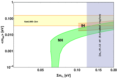
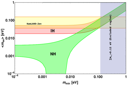
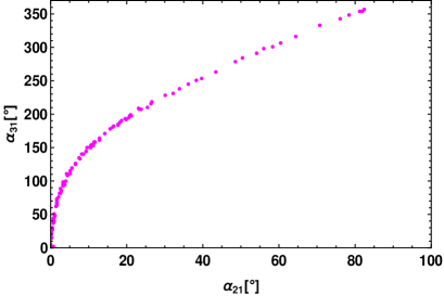
Figure 4: Upper left panel shows the correlation in the plane of effective mass parameter $\langle m_{ee}\rangle$ and $\sum m_{\nu_{i}}$, whereas, upper right panel projects the correlation of $\langle m_{ee}\rangle$ and with lightest neutrino mass $m_{1}$ (i.e., $m_{min}$). Lower panel shows the correlation Majorana phases $\alpha_{21}$ and $\alpha_{31}$.

The right panel of Fig. 3 represents the Feynman diagram due the exchange of the heavy neutrinos $\Sigma_{Ri}$ consisting all the relevant vertex couplings Dash:2021pbx whose relevance is seen in numerical deductions, due to which the effective mass parameter $\langle m_{ee}\rangle$ receives additional contribution. We showcase the results in Fig. 4, wherein the upper left (right) panel reflects the behaviour of $\langle m_{ee}\rangle$ Agostini:2022zub ; King:2013psa w.r.t. sum of neutrino mass ($\sum m_{\nu_{i}}$) (lightest neutrino mass $m_{\rm min})$ Gehrlein:2020jnr ; Barry:2010yk abiding the KamLAND-Zen bound (KamLAND-Zen:2022tow, ) and the bottom panel shows the correlation between Majorana phases i.e., ($\alpha_{21}$ and $\alpha_{31}$).

Fig. 5 shows the dependence of Yukawa couplings on the real and imaginary parts of $\tau$, while keeping the model parameters at their best-fit values. Finally, in Fig. 6 we show the hierarchical nature of the heavy neutrinos which follow the pattern $M_{\Sigma_{R_{1}}}\ll M_{\Sigma_{R_{2}}}\ll M_{\Sigma_{R_{3}}}$.

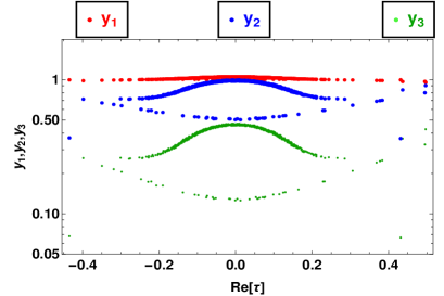
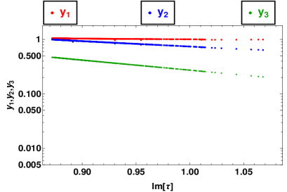
Figure 5: Left (right) panel shows the correlation of the Yukawa couplings i.e., ($y_{1},y_{2},y_{3}$) w.r.t. Re[$\tau$] (Im[$\tau$]), where $y_{1},y_{2}$ and $y_{3},$ are shown in red, blue and green colours respectively.

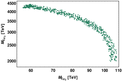
Figure 6: The left (right) plots show the correlation between the heavy neutrino masses i.e., $M_{\Sigma_{R_{1}}}$ and $M_{\Sigma_{R_{2}}}$ ($M_{\Sigma_{R_{2}}}$ and $M_{\Sigma_{R_{3}}}$) in TeV scale.

IV Leptogenesis

Considering the fact that the universe had started from an intially symmetric state of baryons and antibaryons, the present baryon asymmetry can be explained, as suggested by Sakharov Sakharov:1967dj , if the following three criteria are satisfied: Baryon number violation, C and CP violation and departure from thermal equilibrium during the evolution of the universe. Though the SM assures all these criteria for an expanding universe akin ours, the extent of CP violation found in the SM is quite small to accommodate the observed baryon asymmetry of the universe. Therefore, additional sources of CP violation are absolutely essential for explaining this asymmetry. The most common new sources of CP violation possibly could arise in the lepton sector, which is however, not yet firmly established experimentally. Leptogenesis is the phenomenon that furnishes a minimal setup to correlate the CP violation in the lepton sector to the observed baryon asymmetry, as well as imposes indirect constraints on the CP phases from the requirement that it would yield the correct baryon asymmetry. In here, we explore leptogenesis in type-III seesaw model with fermion triplets, where, the lightest heavy fermion is in TeV scale. The general expression for CP asymmetry is mentioned below Hambye:2012fh

$$\epsilon_{CP}=-\sum_{j}\frac{3}{2}\frac{M_{\Sigma_{R_{i}}}}{M_{\Sigma_{R_{j}}}}\frac{\Gamma_{\Sigma_{R_{i}}}}{M_{\Sigma_{R_{j}}}}\left(\frac{V_{j}-2S_{j}}{3}\right)\frac{{\rm Im(\tilde{Y}_{\Sigma}\tilde{Y}_{\Sigma}^{\dagger})^{2}}_{ij}}{{\rm(\tilde{Y}_{\Sigma}\tilde{Y}_{\Sigma}^{\dagger})}_{ii}{\rm(\tilde{Y}_{\Sigma}\tilde{Y}_{\Sigma}^{\dagger})}_{jj}},~{}~{}{\rm with}~{}~{}\tilde{Y}_{\Sigma}=Y_{\Sigma}U_{R},$$ (34)

where, $Y_{\Sigma}=\left({M_{D}}/{v_{u}}\right)$ is the Yukawa matrix of Dirac mass term with its corresponding free parameters given in eqn. (14) and $U_{R}$ being the eigenvector matrix of $M_{R}$ used for its diagonalization i.e., $U_{R}M_{R}U_{R}^{T}\simeq\mathrm{diag}\{M_{\Sigma_{R_{1}}},M_{\Sigma_{R_{2}}},M_{\Sigma_{R_{3}}}\}$. From eqn.(41) it is evident that vertex ($V_{j}$) and self-energy ($S_{j}$) diagrams Hambye:2012fh must contribute to CP asymmetry significantly. However, in the hierarchical limit (i.e., $M_{\Sigma_{R_{1}}}\ll M_{\Sigma_{R_{2,3}}}$ and $M_{\Sigma_{R_{2}}}\neq M_{\Sigma_{R_{3}}}$) they attain the value unity i.e., ($S_{j}=V_{j}=1$). As, we don’t have the hold on fine tuning of the Yukawa couplings, in order to calculate correct lepton asymmetry, we utilize the following benchmark values as shown in Table 5. Moreover, we also show in Fig. 7 the correlation between the one flavor CP asysmmetry i.e., $\epsilon_{CP}$ $\mathcal{O}(10^{-4})$ with the Yukawa couplings within their corresponding ranges i.e., $0.99\lesssim y_{1}\lesssim 1.015$ (upper left panel), $0.4\lesssim y_{2}\lesssim 1.3$ (upper right panel) and $0.1\lesssim y_{3}\lesssim 0.8$ (bottom panel).

$y_{1}$	$y_{2}$	$y_{3}$	$M_{\Sigma_{R_{1}}}$	$\epsilon_{CP}$
$1.0051$	$0.574$	$0.312$	$6.53\times 10^{3}$ $\rm GeV$	$9.713\times 10^{-4}$

Table 5: Benchmark values of the Yukawa couplings and CP asymmetry utilized to generate the correct lepton asymmetry.

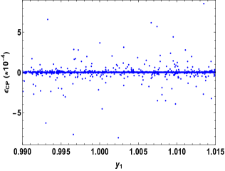
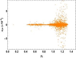
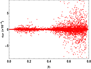
Figure 7: In above we show the correlation of the Yukawa couplings i.e ($y_{1}$, $y_{2}$, $y_{3}$)

w.r.t CP asymmetry i.e., $\epsilon_{CP}$.

IV.1 Boltzmann Equations

The dynamics of applicable Boltzmann equations determine the evolution of particle number densities. The Sakharov conditions Sakharov:1967dj necessitate the decay of the parent heavy fermion, which must be out of equilibrium in order to generate the lepton asymmetry. To do so, one must compare the Hubble expansion rate to the decay rate, as shown below:

$$K_{\Sigma_{R_{i}}}=\frac{\Gamma_{\Sigma_{R_{i}}}}{H(T=M_{\Sigma_{R_{i}}})}.$$ (35)

The Hubble rate is defined as $H=\frac{1.67\sqrt{g_{\star}}~{}T^{2}}{M_{\rm Pl}}$, where, $g_{\star}=106.75$ is the number of relativistic degrees of freedom in the thermal bath and $M_{\rm Pl}=1.22\times 10^{19}$ GeV is the Planck mass. The size of the couplings between the triplet fermions and leptons become the determining factor, guaranteeing that inverse decay does not approach thermal equilibrium. For example, if the value is less than or equal to $10^{-7}$, it gives $K_{\Sigma_{R_{i}}}\sim 1$. The Boltzmann equations associated with evolution of the number densities of right-handed fermion field and lepton can be articulated in terms of the yield parameters, i.e., the ratio of number densities to entropy density, and are expressed as Plumacher:1996kc ; Giudice:2003jh ; Buchmuller:2004nz ; Iso:2010mv

$$\frac{dY_{\Sigma}}{dz}=-\frac{z}{sH(M_{\Sigma})}\left[\left(\frac{Y_{\Sigma}}{{Y^{\rm eq}_{\Sigma}}}-1\right)\gamma_{D}+\left(\left(\frac{{Y_{\Sigma}}}{{Y^{\rm eq}_{\Sigma}}}\right)^{2}-1\right)\gamma_{A}\right],$$

$$\frac{dY_{{B-L}}}{dz}=-\frac{z}{sH(M_{\Sigma})}\left[\frac{Y_{{B-L}}}{{Y^{\rm eq}_{\ell}}}\gamma_{D}-\epsilon_{CP}\left(\frac{Y_{\Sigma}}{{Y^{\rm eq}_{\Sigma}}}-1\right)\frac{\gamma_{D}}{2}\right],$$ (36)

where $z=M_{\Sigma_{R_{i}}}/T$, $s$ is the entropy density, and the equilibrium number densities have the form Davidson:2008bu

$$Y^{\rm eq}_{\Sigma}=\frac{135g_{\Sigma}}{16{\pi}^{4}g_{\star}}z^{2}K_{2}(z),\hskip 8.53581pt{Y^{\rm eq}_{\ell}}=\frac{3}{4}\frac{45\zeta(3)g_{\ell}}{2{\pi}^{4}g_{\star}}\,.$$ (37)

$K_{1,2}$ in Eq. (37) represent the modified Bessel functions, the lepton and RH fermion degrees of freedom take the values $g_{\ell}=2$ and $g_{\Sigma_{R_{i}}}=2$ and the decay rate $\gamma_{D}$ is given as

$$\gamma_{D} = sY^{\rm eq}_{\Sigma}\Gamma_{\Sigma}\frac{K_{1}(z)}{K_{2}(z)},~{}~{}~{}\Gamma_{\Sigma}=\frac{1}{8\pi}M_{\Sigma_{R_{i}}}(\tilde{\rm{Y}}_{\Sigma}^{\dagger}\tilde{\rm{Y}}_{\Sigma})_{ii},$$

$$\gamma_{A} = \frac{M_{\Sigma_{R_{1}}}T^{3}}{32\pi^{3}}e^{-2z}\left[\frac{111g^{4}}{8\pi}+\frac{3}{2z}\left(\frac{111g^{4}}{8\pi}+\frac{51g^{4}}{16\pi}\right)+\mathcal{O}(1/z)^{2}\right],$$ (38)

wherein $\gamma_{A}$ denotes the gauge annihilation process Hambye:2012fh ; Mishra:2020gxg , with $g$ being the typical gauge coupling.

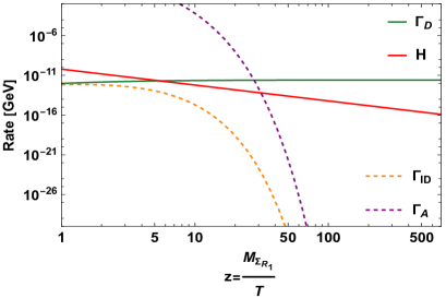
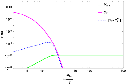
Figure 8: Left panel exhibits the comparison of interaction rates with Hubble expansion rate ($H$) represented by red solid line, where, green solid line corresponds to decay $\left(\Gamma_{D}=\Gamma_{\Sigma}\frac{K_{1}(z)}{K_{2}(z)}\right)$ Davidson:2012fn , inverse decay ($\Gamma_{ID}=\Gamma_{D}\left(\nicefrac{{Y_{\Sigma}^{eq}}}{{Y_{\ell}^{eq}}}\right)$) Strumia:2006qk is shown by dotted orange line and annihilation rate ($\Gamma_{A}$) by dotted purple line. Right panel projects the evolution of $Y_{B-L}$ (green solid line) as a function of $z=\frac{M_{\Sigma_{R_{1}}}}{T}$.

The comparison of the interaction rates with Hubble expansion rate ($H$) is displayed in the left panel of Fig. 8, while the solution of Boltzmann eq. (36) is presented in the right panel. For coupling strength of around ($\simeq~{}10^{-7}$), $Y_{\Sigma}$ (magenta solid curve) with $|Y_{\Sigma}-Y^{\rm eq}_{\Sigma}|$ (blue dashed curve) are shown where the generated lepton asymmetry is around ($\simeq 10^{-10}$) (green thick curve). The lepton asymmetry thus obtained can be converted into baryon asymmetry through the sphaleron transition process, and is given as Plumacher:1996kc ; Vatsyayan:2022rth ; Harvey:1990qw

$$Y_{B}=3\left(\frac{8n_{f}+4n_{H}}{22n_{f}+13n_{H}}\right)Y_{{B-L}},$$ (39)

where, $n_{f}$ represents the number of triplet fermion generations, $n_{H}$ denotes the no. of Higgs doublets and the factor of 3 comes from the three $SU(2)_{L}$ degrees of freedom of the triplets. The observed baryon asymmetry of the universe generally expressed in terms of baryon to photon ratio as Planck:2018vyg

$$\eta=\frac{n_{b}-n_{\bar{b}}}{n_{\gamma}}=6.08\times 10^{-10}.$$ (40)

The current bound on baryon asymmetry AharonyShapira:2021ize can be procured from the relation $Y_{B}=\eta/7.04$ as $Y_{B}=(8.6\pm 0.1)\times 10^{-11}\equiv Y^{obs}_{B}$. Using the asymptotic value of the lepton asymmetry as ($8.77\times 10^{-10}$) from Fig. 8, we obtain the value of baryon asymmetry as $Y_{B}=\frac{24}{23}~{}Y_{B-L}\sim 10^{-10}$.

IV.2 A note on flavor consideration

When ($T>10^{12}$ GeV), one flavor approximation suffices in leptogenesis, indicating that all Yukawa interactions are out of equilibrium. However, at temperatures $\ll 10^{8}$ GeV, various charged lepton Yukawa couplings (i.e., each for three generations) come into equilibrium, making flavor effects a crucial factor in determining the final lepton asymmetry. All Yukawa interactions occur in equilibrium at temperatures below $10^{6}$ GeV, and the asymmetry is encoded in the individual lepton flavor. Numerous studies on flavor effects in type-I leptogenesis can be found in the literature Pascoli:2006ci ; Antusch:2006cw ; Nardi:2006fx ; Abada:2006ea ; Granelli:2020ysj ; Dev:2017trv . The lower bounds on heavy Majorana masses are relaxed when flavour effects are taken into account, giving more room for low scale leptogenesis Abada:2018oly ; Drewes:2022kap ; Alanne:2018brf . Given the significance of flavour effects in low scale leptogenesis, we briefly examine their implications in the current framework in relation to the CP asymmetry for each particular lepton flavour ($\alpha=e,\mu,\tau$) given below Dev:2015cxa ; Mishra:2019gsr

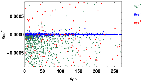
Figure 9: In the above plot the interdependence of CP asymmetry corresponding to each flavor i.e., ($\alpha=e,\mu,\tau$) is been projected against $\delta_{CP}$.

$$\epsilon^{\alpha}_{\Sigma}=\frac{1}{2}\sum_{j}\frac{M_{\Sigma_{R_{i}}}}{M_{\Sigma_{R_{j}}}}\frac{\Gamma_{\Sigma_{R_{i}}}}{M_{\Sigma_{R_{j}}}}\left[\frac{\rm{Im}\left[\left(\tilde{Y}_{\Sigma}\tilde{Y}_{\Sigma}^{\dagger}\right)_{ij}\tilde{Y}_{\alpha i}^{*}\tilde{Y}_{\alpha j}\right]}{{\rm{(\tilde{Y}_{\Sigma}\tilde{Y}_{\Sigma}^{\dagger})}}_{ii}{\rm(\tilde{Y}_{\Sigma}\tilde{Y}_{\Sigma}^{\dagger})}_{jj}}\right],$$ (41)

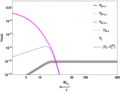
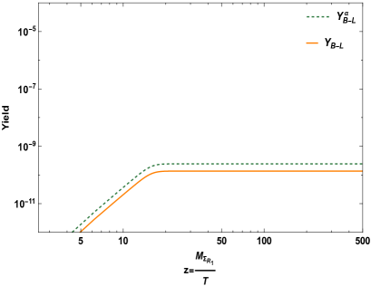
Figure 10: After including the flavor effects the yield is shown in left panel, whereas, right panel displays the yield enhancement due to flavor effects.

The Boltzmann equation describing the generation of $(B-L)$ asymmetry for each lepton flavor is Antusch:2006cw

$$\frac{dY^{\alpha}_{B-L}}{dz}=-\frac{z}{sH(M_{\Sigma})}\left[\epsilon^{\alpha}_{\Sigma}\left(\frac{Y_{\Sigma}}{{Y^{eq}_{\Sigma}}}-1\right)\gamma_{D}-\left(\frac{\gamma^{\alpha}_{D}}{2}\right)\frac{A_{\alpha\alpha}Y^{\alpha}_{\rm B-L_{\alpha}}}{{Y^{eq}_{\ell}}}\right],$$ (42)

where, $\epsilon^{\alpha}_{\Sigma}$ i.e., $(\alpha=e,\mu,\tau)$ represents the CP asymmetry in each lepton flavor

$$\gamma_{D}^{\alpha}=sY_{\Sigma}^{eq}\Gamma_{\Sigma}^{\alpha}\frac{K_{1}(z)}{K_{2}(z)},\quad\gamma_{D}=\sum_{\alpha}\gamma^{\alpha}_{D}.\\$$

The matrix $A$ is given by Nardi:2006fx ,

$${A}=\begin{pmatrix}-\frac{221}{711}&&\frac{16}{711}&&\frac{16}{711}\\ \frac{16}{711}&&-\frac{221}{711}&&\frac{16}{711}\\ \frac{16}{711}&&\frac{16}{711}&&-\frac{221}{711}\\ \end{pmatrix}.\\$$

In addition to which we have expressed a plot to show the interdependence of each flavor on $\delta_{CP}$ in Fig. 9. Subsequently, for the flavor case, benchmark values of CP asymmetry associated with ($e,\mu,\tau$) flavors are $\epsilon_{\Sigma}^{e}=4.7\times 10^{-4}$, $\epsilon_{\Sigma}^{\mu}=5.6\times 10^{-4}$ and $\epsilon_{\Sigma}^{\tau}=7.2\times 10^{-4}$ respectively. Therefore, we estimate the $B-L$ yield with flavor consideration in the left panel of Fig. 10. It is quite obvious to notice that the enhancement in $B-L$ asymmetry is obtained in case of flavor consideration (green dashed line) over the one flavor approximation (orange solid line), as displayed in the right panel. This is because, in one flavor approximation the decay of the heavy fermion to a particular lepton flavor final state can get washed away by the inverse decays of any flavor unlike the flavored case Abada:2006ea .

V Collider Bound on $Z^{\prime}$ mass

As previously mentioned in Sec II, the $U(1)_{B-L}$ gauge symmetry is spontaneously broken by assigning the vacuum expectation value $v_{\rho}$ to the singlet scalar $\rho$. Consequently, the neutral gauge boson $Z^{\prime}$ associated with this symmetry becomes massive by absorbing the massless pseudoscalar component of $\rho$ and its mass is given as,

$$M_{Z^{\prime}}=g_{BL}v_{\rho}\;,$$ (43)

where, $g_{BL}$ is the gauge coupling constant of $U(1)_{B-L}$. The LEP-II provides the constraint on the ratio of mass of $Z^{\prime}$ boson to its coupling as $M_{Z^{\prime}}/g_{BL}>6.9$ TeV ALEPH:2013dgf . Hence, in this work we have considered the range of the $v_{\rho}$ as [$10^{3}-10^{4}$] TeV (28), consistent with the LEP-II bound.

The ATLAS and CMS collaborations have performed extensive searches for the new resonances in both dilepton and dijet channels. In the absence of any excess events over the SM background, they put lower bounds on the mass of $Z^{\prime}$ boson. These bounds are usually limited to a specific model, and typically the experiments report their results assuming simplified models, like the Sequential Standard Model (SSM) or GUT-inspired $E_{6}$ models.

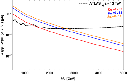
Figure 11: The colored lines represent the dilepton signal cross sections for $pp\to Z^{\prime}\to ee(\mu\mu)$ as a function of $M_{Z^{\prime}}$ for a representative set of $g_{BL}$ values and the black dashed line symbolizes the ATLAS bound ATLAS:2019erb .

Recent results from ATLAS ATLAS:2019erb , provide the lower limits on the $Z^{\prime}$ mass from the dilepton search using Run 2 data, collected with the center of mass energy $\sqrt{s}=13$ TeV. In this work, we use CalcHEP Belyaev:2012qa to compute the production cross section of $Z^{\prime}$, i.e., $pp\to Z^{\prime}\to ee(\mu\mu)$. In Fig. 11, we show the $Z^{\prime}$ production cross section times the branching fraction of $Z^{\prime}$ decaying to dilepton ($ee,\mu\mu$) signal as a function of $M_{Z^{\prime}}$, for some representative values of the gauge coupling $g_{BL}=0.03,0.08,0.11$. The black dashed line denotes the dilepton bound from ATLAS ATLAS:2019erb . It can be noticed from the figure that the region below $M_{Z^{\prime}}\simeq$ 1.3 TeV is excluded for $g_{BL}=0.03$ in red color. For $g_{BL}=0.08$, $M_{Z^{\prime}}<2.47$ TeV in blue color is ruled out and the mass region of $M_{Z^{\prime}}>2.69$ TeV is allowed for $g_{BL}=0.11$ in orange color. Thus, one can generalize these observations as the lower limits on $M_{Z^{\prime}}$ increases with the increase of the gauge couplings.

VI Conclusion

We have curated a model involving $\rm A_{4}$ modular symmetry and $U(1)_{B-L}$ gauged symmetry using type-III seesaw mechanism in super-symmetric context in order to realize the neutrino phenomenology and to explain the observed oscillation data. We have incorporated $SU(2)_{L}$ triplet fermions ($\Sigma$) along with a singlet weighton field ($\rho$). The Yukawa couplings acquire modular forms under $A_{4}$ modular discrete symmetry, where, acquisition of VEV by modulus $\tau$ breaks $A_{4}$ symmetry. This discrete symmetry is useful in procuring a definite neutrino mass matrix structure. Here, in analysis section numerical diagonalization technique lessens the burden and the predicted results are in accordance to the 3$\sigma$ bound as obtained through several experiments. We can extract the best fit values for the model parameters using the chi-square minimization approach, which helps us find strong correlations between the observables. As a consequence, we obtain the sum of active neutrino masses $\sum m_{\nu_{i}}$ within $[0.058-0.12]$ eV and mixing angles are seen to be within their 3$\sigma$ ranges. The model engenders neutrinoless double beta decay mass parameter $\langle m_{ee}\rangle$ between 0.0039 and 0.0087, which assures the limit coming from KamLAND-Zen experiment. Also, Majorana phases $\alpha_{21}$ and $\alpha_{31}$ are revealed in the range $[0^{\circ},80^{\circ}]$ and $[0^{\circ},360^{\circ}]$ respectively. Proceeding further, the results for $\delta_{\rm CP}$ and Jarlskog invariant $J_{\rm CP}$ is seen to be within $[202^{\circ},211^{\circ}]$ and [5.5,7.1] $\times 10^{-3}$ respectively establishing a strong correlation. Further, as there is an hierarchical mass difference between the heavy fermions ($M_{\Sigma}$) in the model with $M_{\Sigma_{R_{1}}}$, $M_{\Sigma_{R_{2}}}$ and $M_{\Sigma_{R_{3}}}$ are found to be within the range [$6-8.5$] TeV, [$50-110$] TeV and [$2000-4500$] TeV respectively, hence, the decay of lightest one gives rise to non-zero CP asymmetry. The lepton asymmetry coming from Boltzmann equation is $\simeq$ $10^{-10}$, and hence explains the baryon asymmetry of the Universe and also we have discussed the flavor effects as our lightest heavy fermion is in TeV scale. Additionally, we have discussed the mass of the new neutral $Z^{\prime}$ gauge boson associated with $U(1)_{B-L}$ symmetry which is within the present experimental collider bounds.

Appendix A $A_{4}$ modular symmetry

$\rm A_{4}$ group is the alternating group of even permutations of four entries. It is isomorphic to the tetrahedral symmetry. The generators of the group S and T, following the relations,

$$S^{2}=(TS)^{3}=(ST)^{3}=\mathbb{I}.$$ (44)

Group formed by the generators S and T is the inhomogeneous modular group $\bar{\Gamma}$ and the transformations are abbreviated as follows (King:2020qaj, ; feruglio2019neutrino, )

$$S:\tau\rightarrow\frac{-1}{\tau},\hskip 56.9055ptT:\tau\rightarrow\tau+1$$ (45)

Representation of S and T in the SL(2,$\mathbb{Z}$ ) group is,

$$S=\begin{pmatrix}0&1\\ -1&0\end{pmatrix},\hskip 56.9055ptT=\begin{pmatrix}1&1\\ 0&1\end{pmatrix}.$$ (46)

A group of linear fractional transformations forms the modular group, which transforms the modulus $\tau$ in the upper half-plane [Im($\tau$) $>$ 0],

$$\tau\rightarrow\frac{c\tau+d}{a\tau+b},\hskip 56.9055pt(a,b,c,d\hskip 2.84526ptare\hskip 2.84526ptintegers,\hskip 28.45274ptcb-da=1)$$ (47)

and the mapping,

$$\frac{c\tau+d}{a\tau+b}\rightarrow\begin{pmatrix}c&d\\ a&b\end{pmatrix},$$ (48)

is an isomorphism from the modular group. Following is the series of groups $\Gamma(N)$, where N=1, 2, 3…,

$$\Gamma(N)=\Big{\{}\begin{pmatrix}c&d\\ a&b\end{pmatrix}\in SL(2,\mathbb{Z}),\hskip 5.69054pt\begin{pmatrix}c&d\\ a&b\end{pmatrix}=\begin{pmatrix}1&0\\ 0&1\end{pmatrix}\Big{\}},$$ (49)

where, $\Gamma$ = SL(2,$\mathbb{Z}$ ) is homogeneous modular group and $\Gamma$(N). The group $\Gamma$(N) operates on the complex modulus $\tau$, in the upper half plane as the linear fractional transformation,

$$\gamma=\frac{c\tau+d}{a\tau+b}.$$ (50)

A significant modular invariant element is the modular function $f(\tau)$ which is holomorphic function of $\tau$ with level N and modular weight 2k, under $\Gamma(N)$ is,

$$f\Big{(}\frac{c\tau+d}{a\tau+b}\Big{)}=(a\tau+b)^{2k}f(\tau),\hskip 5.69054pt\forall\begin{pmatrix}c&d\\ a&b\end{pmatrix}=\gamma\in{\Gamma}(N).$$ (51)

Here, N can vary according to the symmetry group $\rm A_{4}$, $\rm S_{3}$, $\rm S_{4}$, or $\rm A_{5}$. In reference (King:2020qaj, ), it is given that for N = 2, 3, 4, and 5; $\Gamma_{2}$, $\Gamma_{3}$, $\Gamma_{4}$ and $\Gamma_{5}$ are isomorphic to $\rm S_{3}$, $\rm A_{4}$, $\rm S_{4}$, and $\rm A_{5}$ respectively. The modular forms of $A_{4}$ triplet Yukawa couplings read as,

$$Y_{1}(\tau) = \frac{i}{2\pi}\left[\frac{\eta^{\prime}(\frac{\tau}{3})}{\eta(\frac{\tau}{3})}+\frac{\eta^{\prime}(\frac{\tau+1}{3})}{\eta(\frac{\tau+1}{3})}+\frac{\eta^{\prime}(\frac{\tau+2}{3})}{\eta(\frac{\tau+2}{3})}-\frac{27\eta^{\prime}(3\tau)}{\eta({3\tau})}\right]$$ (52)

$$Y_{2}(\tau) = \frac{-i}{\pi}\left[\frac{\eta^{\prime}(\frac{\tau}{3})}{\eta(\frac{\tau}{3})}+\omega^{2}\frac{\eta^{\prime}(\frac{\tau+1}{3})}{\eta(\frac{\tau+1}{3})}+\omega\frac{\eta^{\prime}(\frac{\tau+2}{3})}{\eta(\frac{\tau+2}{3})}\right]$$ (53)

$$Y_{2}(\tau) = \frac{-i}{\pi}\left[\frac{\eta^{\prime}(\frac{\tau}{3})}{\eta(\frac{\tau}{3})}+\omega\frac{\eta^{\prime}(\frac{\tau+1}{3})}{\eta(\frac{\tau+1}{3})}+\omega^{2}\frac{\eta^{\prime}(\frac{\tau+2}{3})}{\eta(\frac{\tau+2}{3})}\right]$$ (54)

where $\eta(\tau)$ is Dedekind eta-function which can be defined in the upper half plane of the complex plane.

$$\eta(\tau)=q^{1/24}\prod_{m=1}^{\infty}(1-q^{m})~{}~{}~{}~{}~{}~{}~{}~{}q=e^{\iota 2\pi\tau}$$ (55)

References

- (1) E. Ma, Pathways to naturally small neutrino masses, Phys. Rev. Lett. 81 (1998) 1171 [hep-ph/9805219].
- (2) S. Weinberg, Baryon and Lepton Nonconserving Processes, Phys. Rev. Lett. 43 (1979) 1566.
- (3) A. Abada, C. Biggio, F. Bonnet, M.B. Gavela and T. Hambye, Low energy effects of neutrino masses, JHEP 12 (2007) 061 [arXiv:0707.4058].
- (4) P. Minkowski, at a Rate of One Out of Muon Decays?, Phys. Lett. B 67 (1977) 421.
- (5) T. Yanagida, Horizontal gauge symmetry and masses of neutrinos, Conf. Proc. C 7902131 (1979) 95.
- (6) S.L. Glashow, The Future of Elementary Particle Physics, NATO Sci. Ser. B 61 (1980) 687.
- (7) R.N. Mohapatra and G. Senjanovic, Neutrino Mass and Spontaneous Parity Nonconservation, Phys. Rev. Lett. 44 (1980) 912.
- (8) R.N. Mohapatra and G. Senjanovic, Neutrino Masses and Mixings in Gauge Models with Spontaneous Parity Violation, Phys. Rev. D 23 (1981) 165.
- (9) S. Antusch and S.F. King, Type II Leptogenesis and the neutrino mass scale, Phys. Lett. B 597 (2004) 199 [hep-ph/0405093].
- (10) P.H. Gu, H. Zhang and S. Zhou, A Minimal Type II Seesaw Model, Phys. Rev. D 74 (2006) 076002 [hep-ph/0606302].
- (11) A. Arhrib, R. Benbrik, M. Chabab, G. Moultaka, M.C. Peyranere, L. Rahili et al., The Higgs Potential in the Type II Seesaw Model, Phys. Rev. D 84 (2011) 095005 [arXiv:1105.1925].
- (12) D.K. Ghosh, N. Ghosh, I. Saha and A. Shaw, Revisiting the high-scale validity of the type II seesaw model with novel LHC signature, Phys. Rev. D 97 (2018) 115022 [arXiv:1711.06062].
- (13) R. Foot, H. Lew, X.G. He and G.C. Joshi, Seesaw Neutrino Masses Induced by a Triplet of Leptons, Z. Phys. C 44 (1989) 441.
- (14) Y. Liao, J.Y. Liu and G.Z. Ning, Radiative Neutrino Mass in Type III Seesaw Model, Phys. Rev. D 79 (2009) 073003 [arXiv:0902.1434].
- (15) E. Ma, Deciphering the Seesaw Nature of Neutrino Mass from Unitarity Violation, Mod. Phys. Lett. A 24 (2009) 2161 [arXiv:0904.1580].
- (16) W. Wang and Z.L. Han, Radiative linear seesaw model, dark matter, and , Phys. Rev. D 92 (2015) 095001 [arXiv:1508.00706].
- (17) D. Borah and B. Karmakar, Linear seesaw for Dirac neutrinos with flavour symmetry, Phys. Lett. B 789 (2019) 59 [arXiv:1806.10685].
- (18) A.E. Cárcamo Hernández, L.T. Hue, S. Kovalenko and H.N. Long, An extended 3-3-1 model with two scalar triplets and linear seesaw mechanism, Eur. Phys. J. Plus 136 (2021) 1158 [arXiv:2001.01748].
- (19) M. Sruthilaya, R. Mohanta and S. Patra, realization of Linear Seesaw and Neutrino Phenomenology, Eur. Phys. J. C 78 (2018) 719 [arXiv:1709.01737].
- (20) M. Hirsch, S. Morisi and J.W.F. Valle, A4-based tri-bimaximal mixing within inverse and linear seesaw schemes, Phys. Lett. B 679 (2009) 454 [arXiv:0905.3056].
- (21) P.H. Gu and U. Sarkar, Leptogenesis with Linear, Inverse or Double Seesaw, Phys. Lett. B 694 (2011) 226 [arXiv:1007.2323].
- (22) A. Das and N. Okada, Inverse seesaw neutrino signatures at the LHC and ILC, Phys. Rev. D 88 (2013) 113001 [arXiv:1207.3734].
- (23) E. Arganda, M.J. Herrero, X. Marcano and C. Weiland, Imprints of massive inverse seesaw model neutrinos in lepton flavor violating Higgs boson decays, Phys. Rev. D 91 (2015) 015001 [arXiv:1405.4300].
- (24) A.G. Dias, C.A. de S. Pires, P.S. Rodrigues da Silva and A. Sampieri, A Simple Realization of the Inverse Seesaw Mechanism, Phys. Rev. D 86 (2012) 035007 [arXiv:1206.2590].
- (25) P.S.B. Dev and A. Pilaftsis, Minimal Radiative Neutrino Mass Mechanism for Inverse Seesaw Models, Phys. Rev. D 86 (2012) 113001 [arXiv:1209.4051].
- (26) A.G. Dias, C.A. de S. Pires and P.S.R. da Silva, How the Inverse See-Saw Mechanism Can Reveal Itself Natural, Canonical and Independent of the Right-Handed Neutrino Mass, Phys. Rev. D 84 (2011) 053011 [arXiv:1107.0739].
- (27) F. Bazzocchi, Minimal Dynamical Inverse See Saw, Phys. Rev. D 83 (2011) 093009 [arXiv:1011.6299].
- (28) S.M. Barr, A Different seesaw formula for neutrino masses, Phys. Rev. Lett. 92 (2004) 101601 [hep-ph/0309152].
- (29) C.H. Albright and S.M. Barr, Leptogenesis in the type III seesaw mechanism, Phys. Rev. D 69 (2004) 073010 [hep-ph/0312224].
- (30) E. Ma, Non-Abelian discrete symmetries and neutrino masses: Two examples, New J. Phys. 6 (2004) 104 [hep-ph/0405152].
- (31) J. Kubo, A. Mondragon, M. Mondragon and E. Rodriguez-Jauregui, The Flavor symmetry, Prog. Theor. Phys. 109 (2003) 795 [hep-ph/0302196].
- (32) S. Pakvasa and H. Sugawara, Discrete Symmetry and Cabibbo Angle, Phys. Lett. B 73 (1978) 61.
- (33) E. Ma and R. Srivastava, Dirac or inverse seesaw neutrino masses with gauge symmetry and flavor symmetry, Phys. Lett. B 741 (2015) 217 [arXiv:1411.5042].
- (34) E. Ma and G. Rajasekaran, Softly broken A(4) symmetry for nearly degenerate neutrino masses, Phys. Rev. D 64 (2001) 113012 [hep-ph/0106291].
- (35) K.S. Babu, E. Ma and J.W.F. Valle, Underlying A(4) symmetry for the neutrino mass matrix and the quark mixing matrix, Phys. Lett. B 552 (2003) 207 [hep-ph/0206292].
- (36) G. Altarelli and F. Feruglio, Tri-bimaximal neutrino mixing from discrete symmetry in extra dimensions, Nucl. Phys. B 720 (2005) 64 [hep-ph/0504165].
- (37) E. Ma, A(4) symmetry and neutrinos with very different masses, Phys. Rev. D 70 (2004) 031901 [hep-ph/0404199].
- (38) E. Ma, Neutrino mass matrix from S(4) symmetry, Phys. Lett. B 632 (2006) 352 [hep-ph/0508231].
- (39) R. Krishnan, P.F. Harrison and W.G. Scott, Simplest Neutrino Mixing from S4 Symmetry, JHEP 04 (2013) 087 [arXiv:1211.2000].
- (40) W. Grimus, L. Lavoura and P.O. Ludl, Is S(4) the horizontal symmetry of tri-bimaximal lepton mixing?, J. Phys. G 36 (2009) 115007 [arXiv:0906.2689].
- (41) S. Mishra, M.K. Behera, R. Mohanta, S. Patra and S. Singirala, Neutrino phenomenology and dark matter in an flavour extended model, Eur. Phys. J. C 80 (2020) 420 [arXiv:1907.06429].
- (42) E. Ma and R. Srivastava, Dirac or inverse seesaw neutrino masses from gauged symmetry, Mod. Phys. Lett. A 30 (2015) 1530020 [arXiv:1504.00111].
- (43) S. Singirala, R. Mohanta and S. Patra, Singlet scalar Dark matter in models without right-handed neutrinos, Eur. Phys. J. Plus 133 (2018) 477 [arXiv:1704.01107].
- (44) S. Singirala, R. Mohanta, S. Patra and S. Rao, Majorana Dark Matter in a new model, JCAP 11 (2018) 026 [arXiv:1710.05775].
- (45) T. Nomura and H. Okada, Neutrinophilic two Higgs doublet model with dark matter under an alternative gauge symmetry, Eur. Phys. J. C 78 (2018) 189 [arXiv:1708.08737].
- (46) T. Nomura and H. Okada, Radiative neutrino mass in an alternative gauge symmetry, Nucl. Phys. B 941 (2019) 586 [arXiv:1705.08309].
- (47) T. Nomura and H. Okada, A radiative seesaw model with higher order terms under an alternative , Phys. Lett. B 781 (2018) 561 [arXiv:1711.05115].
- (48) M.K. Behera, P. Panda, P. Mishra, S. Singirala and R. Mohanta, Exploring Neutrino Masses and Mixing in the Seesaw Model with Gauged Symmetry, arXiv:2108.04066.
- (49) R. Foot, New Physics From Electric Charge Quantization?, Mod. Phys. Lett. A 6 (1991) 527.
- (50) P. Panda, P. Mishra, M.K. Behera and R. Mohanta, Neutrino phenomenology, muon and electron (g-2) under gauged symmetries in an extended inverse seesaw model, arXiv:2203.14536.
- (51) X.G. He, G.C. Joshi, H. Lew and R.R. Volkas, Simplest Z-prime model, Phys. Rev. D 44 (1991) 2118.
- (52) E. Nardi, Horizontal symmetry: a non-anomalous model, PoS silafae-III (2000) 023 [hep-ph/0009329].
- (53) L.E. Ibanez and G.G. Ross, Fermion masses and mixing angles from gauge symmetries, Phys. Lett. B 332 (1994) 100 [hep-ph/9403338].
- (54) P. Binetruy and P. Ramond, Yukawa textures and anomalies, Phys. Lett. B 350 (1995) 49 [hep-ph/9412385].
- (55) Y. Nir, Gauge unification, Yukawa hierarchy and the mu problem, Phys. Lett. B 354 (1995) 107 [hep-ph/9504312].
- (56) S. Ferrara, D. Lust, A.D. Shapere and S. Theisen, Modular Invariance in Supersymmetric Field Theories, Phys. Lett. B 225 (1989) 363.
- (57) S. Ferrara, .D. Lust and S. Theisen, Target Space Modular Invariance and Low-Energy Couplings in Orbifold Compactifications, Phys. Lett. B 233 (1989) 147.
- (58) G.K. Leontaris and N.D. Tracas, Modular weights, U(1)’s and mass matrices, Phys. Lett. B 419 (1998) 206 [hep-ph/9709510].
- (59) F. Feruglio, Are neutrino masses modular forms?, in From My Vast Repertoire… Guido Altarelli’s Legacy, p. 227. World Scientific, 2019.
- (60) S.J.D. King and S.F. King, Fermion mass hierarchies from modular symmetry, JHEP 09 (2020) 043 [arXiv:2002.00969].
- (61) H. Okada and Y. Orikasa, Modular symmetric radiative seesaw model, Phys. Rev. D 100 (2019) 115037 [arXiv:1907.04716].
- (62) T. Kobayashi, K. Tanaka and T.H. Tatsuishi, Neutrino mixing from finite modular groups, Phys. Rev. D 98 (2018) 016004 [arXiv:1803.10391].
- (63) T. Kobayashi, Y. Shimizu, K. Takagi, M. Tanimoto, T.H. Tatsuishi and H. Uchida, Finite modular subgroups for fermion mass matrices and baryon/lepton number violation, Phys. Lett. B 794 (2019) 114 [arXiv:1812.11072].
- (64) T. Kobayashi, Y. Shimizu, K. Takagi, M. Tanimoto and T.H. Tatsuishi, Modular -invariant flavor model in SU(5) grand unified theory, PTEP 2020 (2020) 053B05 [arXiv:1906.10341].
- (65) M.K. Behera, S. Singirala, S. Mishra and R. Mohanta, A modular A 4 symmetric scotogenic model for neutrino mass and dark matter, J. Phys. G 49 (2022) 035002 [arXiv:2009.01806].
- (66) T. Nomura, H. Okada and Y. Shoji, models with modular symmetry, arXiv:2206.04466.
- (67) M. Kashav and S. Verma, On Minimal realization of Topological Lorentz Structures with one-loop Seesaw extensions in A4 Modular Symmetry, arXiv:2205.06545.
- (68) M. Kashav and S. Verma, Broken scaling neutrino mass matrix and leptogenesis based on A4 modular invariance, JHEP 09 (2021) 100 [arXiv:2103.07207].
- (69) M.K. Behera, S. Mishra, S. Singirala and R. Mohanta, Implications of modular symmetry on Neutrino mass, Mixing and Leptogenesis with Linear Seesaw, arXiv:2007.00545.
- (70) T. Asaka, Y. Heo and T. Yoshida, Lepton flavor model with modular symmetry in large volume limit, Phys. Lett. B 811 (2020) 135956 [arXiv:2009.12120].
- (71) M. Abbas, Modular Invariance Model for Lepton Masses and Mixing, Phys. Atom. Nucl. 83 (2020) 764.
- (72) H. Okada and Y. Shoji, A radiative seesaw model with three Higgs doublets in modular symmetry, Nucl. Phys. B 961 (2020) 115216 [arXiv:2003.13219].
- (73) G. Altarelli and F. Feruglio, Tri-bimaximal neutrino mixing, A(4) and the modular symmetry, Nucl. Phys. B 741 (2006) 215 [hep-ph/0512103].
- (74) T. Kobayashi, Y. Shimizu, K. Takagi, M. Tanimoto and T.H. Tatsuishi, lepton flavor model and modulus stabilization from modular symmetry, Phys. Rev. D 100 (2019) 115045 [arXiv:1909.05139].
- (75) X. Wang and S. Zhou, The minimal seesaw model with a modular S4 symmetry, JHEP 05 (2020) 017 [arXiv:1910.09473].
- (76) H. Okada and Y. Orikasa, Neutrino mass model with a modular symmetry, arXiv:1908.08409.
- (77) S.F. King and Y.L. Zhou, Trimaximal TM1 mixing with two modular groups, Phys. Rev. D 101 (2020) 015001 [arXiv:1908.02770].
- (78) T. Kobayashi, Y. Shimizu, K. Takagi, M. Tanimoto and T.H. Tatsuishi, New lepton flavor model from modular symmetry, JHEP 02 (2020) 097 [arXiv:1907.09141].
- (79) P.P. Novichkov, J.T. Penedo, S.T. Petcov and A.V. Titov, Modular S4 models of lepton masses and mixing, JHEP 04 (2019) 005 [arXiv:1811.04933].
- (80) J.T. Penedo and S.T. Petcov, Lepton Masses and Mixing from Modular Symmetry, Nucl. Phys. B 939 (2019) 292 [arXiv:1806.11040].
- (81) J.C. Criado, F. Feruglio and S.J.D. King, Modular Invariant Models of Lepton Masses at Levels 4 and 5, JHEP 02 (2020) 001 [arXiv:1908.11867].
- (82) P.P. Novichkov, J.T. Penedo, S.T. Petcov and A.V. Titov, Modular A5 symmetry for flavour model building, JHEP 04 (2019) 174 [arXiv:1812.02158].
- (83) G.J. Ding, S.F. King and X.G. Liu, Neutrino mass and mixing with modular symmetry, Phys. Rev. D 100 (2019) 115005 [arXiv:1903.12588].
- (84) M.K. Behera and R. Mohanta, Inverse seesaw in modular symmetry, J. Phys. G 49 (2022) 045001 [arXiv:2108.01059].
- (85) M.K. Behera and R. Mohanta, Linear seesaw in modular symmetry with Leptogenesis, arXiv:2201.10429.
- (86) C.Y. Yao, X.G. Liu and G.J. Ding, Fermion masses and mixing from the double cover and metaplectic cover of the modular group, Phys. Rev. D 103 (2021) 095013 [arXiv:2011.03501].
- (87) X. Wang, B. Yu and S. Zhou, Double covering of the modular group and lepton flavor mixing in the minimal seesaw model, Phys. Rev. D 103 (2021) 076005 [arXiv:2010.10159].
- (88) S. Davidson, E. Nardi and Y. Nir, Leptogenesis, Phys. Rept. 466 (2008) 105 [arXiv:0802.2962].
- (89) M. Fukugita and T. Yanagida, Baryogenesis Without Grand Unification, Phys. Lett. B 174 (1986) 45.
- (90) S. Antusch and V. Maurer, Running quark and lepton parameters at various scales, JHEP 11 (2013) 115 [arXiv:1306.6879].
- (91) H. Okada and M. Tanimoto, Towards unification of quark and lepton flavors in modular invariance, Eur. Phys. J. C 81 (2021) 52 [arXiv:1905.13421].
- (92) F. Björkeroth, F.J. de Anda, I. de Medeiros Varzielas and S.F. King, Towards a complete A SU(5) SUSY GUT, JHEP 06 (2015) 141 [arXiv:1503.03306].
- (93) I. Esteban, M.C. Gonzalez-Garcia, M. Maltoni, T. Schwetz and A. Zhou, The fate of hints: updated global analysis of three-flavor neutrino oscillations, JHEP 09 (2020) 178 [arXiv:2007.14792].
- (94) KamLAND-Zen collaboration, A. Gando et al., Search for Majorana Neutrinos near the Inverted Mass Hierarchy Region with KamLAND-Zen, Phys. Rev. Lett. 117 (2016) 082503 [arXiv:1605.02889].
- (95) B. Roe, Chi-square Fitting When Overall Normalization is a Fit Parameter, arXiv:1506.09077.
- (96) G.J. Ding, S.F. King and J.N. Lu, SO(10) models with A4 modular symmetry, JHEP 11 (2021) 007 [arXiv:2108.09655].
- (97) P.P. Novichkov, J.T. Penedo and S.T. Petcov, Double cover of modular for flavour model building, Nucl. Phys. B 963 (2021) 115301 [arXiv:2006.03058].
- (98) Planck collaboration, N. Aghanim et al., Planck 2018 results. VI. Cosmological parameters, Astron. Astrophys. 641 (2020) A6 [arXiv:1807.06209].
- (99) S. Roy Choudhury and S. Hannestad, Updated results on neutrino mass and mass hierarchy from cosmology with Planck 2018 likelihoods, JCAP 07 (2020) 037 [arXiv:1907.12598].
- (100) A. Nucciotti, Double beta decay: Experiments and theory review, eConf C070512 (2007) 025 [arXiv:0707.2216].
- (101) KATRIN collaboration, R.G.H. Robertson, KATRIN: an experiment to determine the neutrino mass from the beta decay of tritium, in Community Summer Study 2013: Snowmass on the Mississippi, 7, 2013, arXiv:1307.5486.
- (102) L. Cardani, Neutrinoless Double Beta Decay Overview, SciPost Phys. Proc. 1 (2019) 024 [arXiv:1810.12828].
- (103) M.J. Dolinski, A.W.P. Poon and W. Rodejohann, Neutrinoless Double-Beta Decay: Status and Prospects, Ann. Rev. Nucl. Part. Sci. 69 (2019) 219 [arXiv:1902.04097].
- (104) T. Asaka, S. Eijima and H. Ishida, Mixing of Active and Sterile Neutrinos, JHEP 04 (2011) 011 [arXiv:1101.1382].
- (105) N. Dash, S. Patra, P. Pritimita and U.A. Yajnik, Effect of large light-heavy neutrino mixing and natural type-II seesaw dominance to lepton flavor violation and neutrinoless double beta decay, Eur. Phys. J. C 82 (2022) 847 [arXiv:2105.11795].
- (106) M. Agostini, G. Benato, J.A. Detwiler, J. Menéndez and F. Vissani, Toward the discovery of matter creation with neutrinoless double-beta decay, arXiv:2202.01787.
- (107) S.F. King, A. Merle and A.J. Stuart, The Power of Neutrino Mass Sum Rules for Neutrinoless Double Beta Decay Experiments, JHEP 12 (2013) 005 [arXiv:1307.2901].
- (108) J. Gehrlein and M. Spinrath, Leptonic Sum Rules from Flavour Models with Modular Symmetries, JHEP 03 (2021) 177 [arXiv:2012.04131].
- (109) J. Barry and W. Rodejohann, Neutrino Mass Sum-rules in Flavor Symmetry Models, Nucl. Phys. B 842 (2011) 33 [arXiv:1007.5217].
- (110) KamLAND-Zen collaboration, S. Abe et al., First Search for the Majorana Nature of Neutrinos in the Inverted Mass Ordering Region with KamLAND-Zen, arXiv:2203.02139.
- (111) A.D. Sakharov, Violation of CP Invariance, C asymmetry, and baryon asymmetry of the universe, Pisma Zh. Eksp. Teor. Fiz. 5 (1967) 32.
- (112) T. Hambye, Leptogenesis: beyond the minimal type I seesaw scenario, New J. Phys. 14 (2012) 125014 [arXiv:1212.2888].
- (113) M. Plumacher, Baryogenesis and lepton number violation, Z. Phys. C 74 (1997) 549 [hep-ph/9604229].
- (114) G.F. Giudice, A. Notari, M. Raidal, A. Riotto and A. Strumia, Towards a complete theory of thermal leptogenesis in the SM and MSSM, Nucl. Phys. B 685 (2004) 89 [hep-ph/0310123].
- (115) W. Buchmuller, P. Di Bari and M. Plumacher, Leptogenesis for pedestrians, Annals Phys. 315 (2005) 305 [hep-ph/0401240].
- (116) S. Iso, N. Okada and Y. Orikasa, Resonant Leptogenesis in the Minimal B-L Extended Standard Model at TeV, Phys. Rev. D 83 (2011) 093011 [arXiv:1011.4769].
- (117) S. Mishra, Neutrino mixing and Leptogenesis with modular symmetry in the framework of type III seesaw, arXiv:2008.02095.
- (118) S. Davidson and M. Elmer, Similar Dark Matter and Baryon abundances with TeV-scale Leptogenesis, JHEP 10 (2012) 148 [arXiv:1208.0551].
- (119) A. Strumia, Baryogenesis via leptogenesis, in Les Houches Summer School on Theoretical Physics: Session 84: Particle Physics Beyond the Standard Model, p. 655, 8, 2006, hep-ph/0608347.
- (120) D. Vatsyayan and S. Goswami, Low-scale Fermion Triplet Leptogenesis, arXiv:2208.12011.
- (121) J.A. Harvey and M.S. Turner, Cosmological baryon and lepton number in the presence of electroweak fermion number violation, Phys. Rev. D 42 (1990) 3344.
- (122) S. Aharony Shapira, Current bounds on baryogenesis from complex Yukawa couplings of light fermions, Phys. Rev. D 105 (2022) 095037 [arXiv:2106.05338].
- (123) S. Pascoli, S.T. Petcov and A. Riotto, Leptogenesis and Low Energy CP Violation in Neutrino Physics, Nucl. Phys. B 774 (2007) 1 [hep-ph/0611338].
- (124) S. Antusch, S.F. King and A. Riotto, Flavour-Dependent Leptogenesis with Sequential Dominance, JCAP 11 (2006) 011 [hep-ph/0609038].
- (125) E. Nardi, Y. Nir, E. Roulet and J. Racker, The Importance of flavor in leptogenesis, JHEP 01 (2006) 164 [hep-ph/0601084].
- (126) A. Abada, S. Davidson, A. Ibarra, F.X. Josse-Michaux, M. Losada and A. Riotto, Flavour Matters in Leptogenesis, JHEP 09 (2006) 010 [hep-ph/0605281].
- (127) A. Granelli, K. Moffat and S.T. Petcov, Flavoured resonant leptogenesis at sub-TeV scales, Nucl. Phys. B 973 (2021) 115597 [arXiv:2009.03166].
- (128) P.S.B. Dev, P. Di Bari, B. Garbrecht, S. Lavignac, P. Millington and D. Teresi, Flavor effects in leptogenesis, Int. J. Mod. Phys. A 33 (2018) 1842001 [arXiv:1711.02861].
- (129) A. Abada, G. Arcadi, V. Domcke, M. Drewes, J. Klaric and M. Lucente, Low-scale leptogenesis with three heavy neutrinos, JHEP 01 (2019) 164 [arXiv:1810.12463].
- (130) M. Drewes, Y. Georis, C. Hagedorn and J. Klarić, Low-scale leptogenesis with flavour and CP symmetries, arXiv:2203.08538.
- (131) T. Alanne, T. Hugle, M. Platscher and K. Schmitz, Low-scale leptogenesis assisted by a real scalar singlet, JCAP 03 (2019) 037 [arXiv:1812.04421].
- (132) P.S.B. Dev, TeV Scale Leptogenesis, Springer Proc. Phys. 174 (2016) 245 [arXiv:1506.00837].
- (133) S. Mishra, S. Singirala and S. Sahoo, Scalar dark matter, neutrino mass and leptogenesis in a U(1)B-L model, J. Phys. G 48 (2021) 075003 [arXiv:1908.09187].
- (134) ALEPH, DELPHI, L3, OPAL, LEP Electroweak collaboration, S. Schael et al., Electroweak Measurements in Electron-Positron Collisions at W-Boson-Pair Energies at LEP, Phys. Rept. 532 (2013) 119 [arXiv:1302.3415].
- (135) ATLAS collaboration, G. Aad et al., Search for high-mass dilepton resonances using 139 fb-1 of collision data collected at 13 TeV with the ATLAS detector, Phys. Lett. B 796 (2019) 68 [arXiv:1903.06248].
- (136) A. Belyaev, N.D. Christensen and A. Pukhov, CalcHEP 3.4 for collider physics within and beyond the Standard Model, Comput. Phys. Commun. 184 (2013) 1729 [arXiv:1207.6082].