Joule-Thomson expansion of d-dimensional charged AdS black holes with cloud of strings and quintessence

Abstract

Herein, we focus on the study of Joule-Thomson expansion corresponding to a d-dimensional charged AdS black hole with cloud of strings and quintessence. Then its relevant solution and some thermodynamic properties are investigated. Specifically, we evaluate its Joule-Thomson expansion from four important aspects, including the Joule-Thomson coefficient, inversion curve, isenthalpic curve, and ratio $\frac{T_{i}^{min}}{T_{c}}$. After analysis, different dimensions with strings of cloud and quintessence parameters have different effects on the Joule-Thomson coefficient (the same situation are found for the inversion curve, isenthalpic curve, and ratio $\frac{T_{i}^{min}}{T_{c}}$).

I Introduction

In 1915, Einstein established the general theory of relativity, which describes the gravitational force of spacetime curvature due to the mass presence. The gravitational field equation satisfied by the spacetime gauge is the famous Einstein field equation. Since then, solving various exact solutions of Einstein’s equation has become a hot research topic. Among the various gravitational solutions, it is generally believed that black holes are the best model to link gravitational theory and quantum field theory. The study of black hole physics contributes to the understanding of the nature of gravity and the establishment of quantum gravity theory. In 1916, Schwarzschild solved the first non-trivial exact solution of Einstein’s equations except for flat spacetime, which is a spherically symmetric solution described by just one mass parameter in four-dimensional spacetime. Subsequent studies have mainly considered a black hole as a mathematical property. In 1973, black hole thermodynamics, which connects thermodynamics, classical gravity and quantum mechanics, became a new attractive topic of research. Early, Bekenstein pioneered the black hole entropy, and the black hole was treated as an interesting thermodynamic system Bekenstein:1972tm ; Bardeen:1973gs . In Ref. Bardeen:1973gs the Four laws of black hole were established, then Hawking predicted the thermal emission of radiation (Hawking radiation) Hawking:1974rv ; Hawking:1975vcx ; Hawking:1976de . After that, the complete theory of black hole thermodynamics was developed.

Generally, Einstein’s equation contains a cosmological constant, which is used to describe the state of the universe. If a positive value is imposed on the cosmological constant, the associated negative pressure will be the cause of the accelerated expansion of the universe. Highly astronomical observations suggest that the universe is expanding at an accelerated rate SupernovaCosmologyProject:1998vns ; SupernovaSearchTeam:1998cav , which means there is the negative pressure. In addition to the cosmological constant, the quintessence hypothetical assumed form of dark energy is also an important factor affecting the negative pressure. In the origin of the universe associated with dark energy, the relationship between negative pressure and energy density can be described by an equation of state $p_{q}=\omega_{q}\rho_{q}$, where $q$ stands for quintessence. The origin of the quintessence is related to the dynamic scalar field Ratra:1987rm ; Caldwell:1997ii . The first solution to the Einstein equation associated with the quintessence was obtained by Kiselev in four dimensions Kiselev:2002dx . Next, a solution of Einstein equations with quintessential matter in higher dimensional spacetime was presented Chen:2008ra . After a series of corrections, the solutions of Einstein’s equation about the quintessence were extended to different cases, such as charged black holes Azreg-Ainou:2014lua , $5d$ black hole in Einstein Gauss-Bonnet gravity Ghosh:2016ddh , $d$-dimensional Lovelock gravity Ghosh:2017cuq .

On the other hand, the universe can also be described by a one-dimensional object namely strings. The rapidly accelerating expansion of the universe is also closely linked to the extension of such cosmic strings, which can penetrate anywhere in the universe that one can observe HenryTye:2006uv . String theory treats particles and the fundamental forces of nature as vibrations of tiny supersymmetric strings, and it predicts the existence of quantum gravity. Then, studies on the gravitational effects of matter in the form of string clouds followed, one after another. The connection between the counting string state and the entropy of the black hole was investigated Letelier:1979ej , in which Letelier first studied the general solutions of string clouds satisfying spherical symmetry. The relevant solutions are then generalized to the case in third-order Lovelock gravity Ghosh:2014pga and the case for Einstein-Gauss-Bonnet theory in the Letelier spacetime Herscovich:2010vr . In this context, many other extended solutions for a broad range of black holes have also been studied Richarte:2007bx ; Yadav:2009zza ; Ganguly:2014cqa ; Bronnikov:2016dhz ; Ghosh:2014dqa ; Lee:2014dha .

As the research proceeded, the thermodynamic properties of a variety of complicated black holes attracted attention and were studied Parikh:1999mf ; Kerner:2007rr ; Feng:2015jlj ; Hod:2016hef ; MunozdeNova:2018fxv ; Robson:2018con ; Feng:2018gqr ; Moreno-Ruiz:2019lgn . Among all studies, the thermodynamic behavior in the anti-de Sitter (AdS) space-time with a negative cosmological constant has become a major research topic. Hawking and Page first investigated thermodynamics of the AdS black holes, they also first pointed out the existence of a thermodynamic phase transition between a stable Schwarzschild-AdS black hole and the thermal gas in the AdS space Hawking:1982dh . This work then inspired people to study the common properties between the charged AdS spacetime and general thermodynamic systems Chamblin:1999tk ; Chamblin:1999hg ; Wei:2018pnk ; Banerjee:2011au . It has been shown that there are similarities between RN-AdS black holes and van der Waals fluid phases in terms of phase transition.

In recent years, the cosmological constant has been treated as the thermodynamic pressure, and many studies have been carried out on this basis Caldarelli:1999xj ; Kastor:2009wy ; Kastor:2010gq ; Dolan:2010ha ; Dolan:2011xt ; Cvetic:2010jb ; Yin:2021fsg ; Mu:2021xxx ; Jing:2020sdf ; Mu:2020szg ; Liang:2020uul ; Liang:2020hjz ; Hong:2019yiz . Among these studies, a typical example that deserves attention is the creative introduction of the concept of holographic heat engine, and another interesting example is the introduction of Joule-Thomson expansion (throttling process). Ö. Ökcü and E. Aydıner explored the Joule-Thomson expansion process in the charged AdS black holes and van der Waals system, in which the inversion curves and isenthalpic curves were obtained Okcu:2016tgt . In classical thermodynamics, Joule-Thomson expansion is the process of a high pressure gas passing through a porous plug into a low pressure, during which there is no change in enthalpy. Related studies were subsequently developed to different black holes, such as Kerr-AdS black holes Okcu:2017qgo , AdS black holes with a global monopole RizwanCL:2018cyb , AdS black holes in Lovelock gravity Mo:2018qkt , charged Gauss-Bonnet black holes in AdS space Lan:2018nnp , higher dimensional AdS black holes Mo:2018rgq . These studies further confirm the basic findings in Ref. Okcu:2016tgt . The recent progresses can be found in Refs. Ghaffarnejad:2018exz ; DAlmeida:2018ldi ; Chabab:2018zix ; Liang:2021elg ; Hegde:2020xlv ; Wei:2017vqs ; Kuang:2018goo ; Yekta:2019wmt ; Pu:2019bxf ; Nam:2018sii ; Zhao:2018kpz ; Li:2019jcd ; Hyun:2019gfz ; Ghaffarnejad:2018tpr ; Nam:2019zyk ; Nam:2018ltb ; Rostami:2019ivr ; Haldar:2018cks ; Guo:2019gkr ; Lan:2019kak ; Sadeghi:2020bon ; Bi:2020vcg ; Ranjbari:2019ktp ; Guo:2019pzq ; K.:2020rzl ; Nam:2020gud ; Meng:2020csd ; Guo:2020qxy ; Ghanaatian:2019xhi ; Guo:2020zcr ; Feng:2020swq ; Debnath:2020zdv ; Cao:2021dcq ; Huang:2020xcs ; Zhang:2021raw ; Chen:2020igz ; Jawad:2020mdc ; Liang:2021xny ; Debnath:2020inx ; Mirza:2021kvi ; Graca:2021izb for various other black holes.

This paper is organized as follows: the thermodynamics of the quintessence surrounding d-dimensional Reissner-Nordström-Anti-de Sitter black hole with a cloud of strings is reviewed in Sec. II. The Joule-Thomson expansion of a quintessence surrounding d-dimensional Reissner-Nordström-Anti-de Sitter black hole with a cloud of strings is discussed separately from four aspects in Sec. III. The Joule-Thomson coefficient is investigated in Sec. III.1; the inversion curves are investigated in Sec. III.2; the isenthalpic curves are investigated in Sec. III.3; the ratio between $T_{i}^{min}$ and $T_{c}$ is investigated in Sec. III.4. Finally, the results are discussed in Sec. IV.

II Quintessence surrounding d-dimensional Reissner-Nordström-Anti-de Sitter black holes with a cloud of strings

In this section, we focus on the relevant solution and some thermodynamic properties of a charged AdS black hole surrounded by quintessence with a cloud of strings in higher dimensional spacetime. Under the assumption, the quintessence and cloud of strings have no interaction Chabab:2020ejk ; deMToledo:2018tjq , the spacetime metric corresponding to a d-dimensional charged AdS black holes with cloud of strings and quintessence is given by the general form as follows

$$ds_{d}^{2}=-f(r)dt^{2}+f(r)^{-1}dr^{2}+r^{2}d\varOmega_{d-2}^{2},$$ (1)

the metric function $f(r)$ is given by Chabab:2020ejk

$$f(r)=1-\frac{m}{r^{d-3}}+\frac{q^{2}}{r^{2(d-3)}}-\frac{2\Lambda r^{2}}{(d-2)(d-1)}-\frac{\alpha}{r^{(d-1)\omega_{q}+d-3}}-\frac{2a}{(d-2)r^{d-4}},$$ (2)

where $d\varOmega_{d-2}^{2}$ denotes the metric on unit $(d-2)$-sphere, $\Omega_{d-2}$ is the volume of unit $(d-2)$-sphere, which takes the form deMToledo:2018tjq

$$\varOmega_{d-2}=\frac{2\pi^{\frac{d-1}{2}}}{\Gamma(\frac{d-1}{2})},$$ (3)

here $m$ is the integration constant proportional to the ADM mass, and $q$ is charge of the black hole. There are two related expressions as follows Chamblin:1999tk ; Gunasekaran:2012dq

$$M=\frac{(d-2)}{16\pi}\Omega_{d-2}m,Q=\frac{\sqrt{2(d-2)(d-3)}\varOmega_{d-2}q}{8\pi},$$ (4)

moreover, $a$ in the above is an integration constant related to the presence of cloud of strings. And $\alpha$ is the quintessential parameter (a positive normalization factor), which has a relationship with the energy density for quintessence. The density of quintessence are defined by the equation $\rho_{q}=-\frac{\alpha\omega_{q}(d-1)(d-2)}{4r^{(d-1)(\omega_{q}+1)}}$, with $\omega_{q}$ is barotropic index such that $-1<\omega_{q}<-1/3$. We will set $\omega_{q}=-\frac{d-2}{d-1}$ in numerical analysis for only considering the asymptotically $dS$ behavior. The definition of the cosmological constant is a key definition in the black hole thermodynamic framework. As usual, the cosmological constant is treated as the thermodynamic pressure Dolan:2011xt ; Kubiznak:2012wp ; Cvetic:2010jb ; Caceres:2015vsa ; Hendi:2012um ; Pedraza:2018eey , which is given by

$$P=-\frac{\varLambda}{8\pi}=\frac{3}{8\pi l^{2}}.$$ (5)

On the event horizon $r_{+}$ that corresponds to equation $f(r_{+})=0$, we can obtain the ADM mass

$$M=\frac{(d-2)\Omega_{d-2}r_{+}^{d-3}}{16\pi}+\frac{(d-2)\Omega_{d-2}q^{2}}{16\pi r_{+}^{d-3}}+\frac{\Omega_{d-2}Pr_{+}^{d-1}}{(d-1)}-\frac{\alpha(d-2)\Omega_{d-2}}{16\pi r_{+}^{(d-1)\omega_{q}}}-\frac{ar_{+}\Omega_{d-2}}{8\pi}.$$ (6)

Therefore, the generalized first law of the black hole in the extended phase space is then expressed as

$$dM=TdS+VdP+\phi dQ+\mathcal{A}da+\mathcal{Q}d\alpha,$$ (7)

where

$$\mathcal{Q}=\frac{(2-d)\Omega_{d-2}}{16\pi r_{+}^{(d-1)\omega_{q}}},\mathcal{A}=\frac{-\varOmega_{d-2}r_{+}}{8\pi},$$ (8)

$$\phi=\sqrt{\frac{d-2}{2(d-3)}}\frac{q}{r_{+}^{d-3}},V=\frac{\varOmega_{d-2}r_{+}^{(d-1)}}{d-1}.$$

Above quantities satisfy the generalized Smarr formula as follows

$$M=\frac{d-2}{d-3}TS-\frac{2}{d-3}VP+\phi Q+(\frac{d-1}{d-3}\omega_{q}+1)\mathcal{Q\alpha+\textrm{$\frac{d-4}{d-3}\mathcal{A}a$}}.$$ (9)

With the assistance of Bekenstein-Hawking formula Banerjee:2020xcn , the entropy can be obtained as

$$S=\frac{A_{d-2}}{4}=\frac{\Omega_{d-2}}{4}r_{+}^{d-2}.$$ (10)

Otherwise, the Hawking temperature of the black hole is given by

$$T=(\frac{\partial M}{\partial S})_{P,Q}$$ (11)

$$=\frac{-2ar_{+}^{4-d}-8\pi^{3-d}Q^{2}r_{+}^{6-2d}\Gamma\left(\frac{d-1}{2}\right)^{2}-\alpha(d-2)^{2}r_{+}+(d-5)d+16\pi Pr_{+}^{2}+6}{4\pi(d-2)r_{+}}.$$

III Joule-Thomson expansion

III.1 The Joule-Thomson coefficient

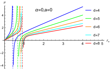
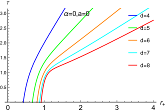
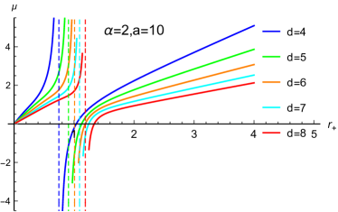
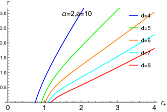
Fig. 1: Joule-Thomson coefficient $\mu$ and Hawking temperature $T$ versus event horizon $r_{+}$. Here, we use $P=1,q=1$.

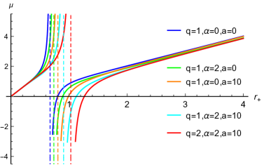
(a) $d=5$

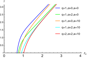
(b) $d=5$

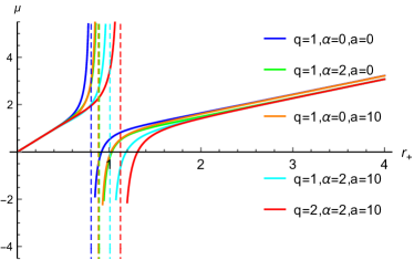
(c) $d=6$

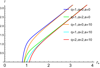
(d) $d=6$

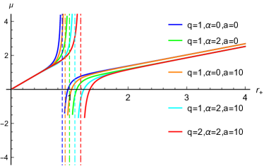
(e) $d=7$

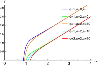
(f) $d=7$

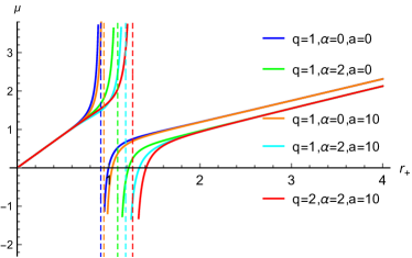
(g) $d=8$

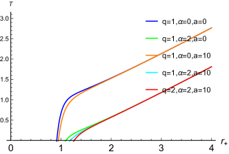
(h) $d=8$

Fig. 2: Joule-Thomson coefficient $\mu$ and Hawking temperature $T$ versus event horizon $r_{+}$ for fixed $P=1$.

In classical thermodynamics, Joule-Thomson expansion describes an adiabatic expansion, which is also called a throttling process. In this process, a nonideal fluid (gas or liquid) expands from a high pressure section to a low pressure section through a porous plug. Besides, the temperature change of the fluid can lead to the cooling or liquefaction of the gas, so the throttling process is widely used in thermal machines including heat pumps, liquefiers, and air conditioners. This process can be considered as an isoenthalpy process, since the enthalpies of the initial and final states of the fluid do remain constant. The main characteristics of the throttling process are adiabatic and isoenthalpic. In the extended phase space, the Hawking radiation of the black hole is usually very tiny that can be regarded as satisfying the adiabatic condition. In addition, when radiation is not considered, the enthalpy of the black hole remains constant, so the process is also isoenthalpic. All above shows that the black hole satisfies the condition of the throttling process. In this process, the change in temperature with respect to pressure can be encoded in the Joule-Thomson coefficient, the sign of which can be used to determine whether heating occurs or cooling occurs. The Joule-Thomson coefficient is as follows

$$\mu=(\frac{\partial T}{\partial P})_{H}.$$ (12)

The negative coefficient $\mu$ corresponds to the heating process of the gas, and the positive coefficient $\mu$ corresponds to the cooling process of the gas. Refs. Okcu:2016tgt ; Okcu:2017qgo derive the Joule-Thomson coefficients in two different ways, and Ref. Mo:2018rgq demonstrates the same result for both methods in a d-dimensional black hole. In this paper we follow the approach proposed in Ref. Okcu:2016tgt . From the first law of thermodynamics and relating it to the differential form of enthalpy, we get

$$dH=TdS+VdP+\phi dQ+\mathcal{A}da+\mathcal{Q}d\alpha.$$ (13)

Using conditions $dH=0$ and $dQ=0$ yields

$$T(\frac{\partial S}{\partial P})_{H}+V=0.$$ (14)

Using the differential form of the entropy of the state function $dS=(\frac{\partial S}{\partial P})_{T,Q,a,\alpha}dP+(\frac{\partial S}{\partial T})_{P,Q,a,\alpha}dT+(\frac{\partial S}{\partial Q})_{T,P,a,\alpha}dQ+(\frac{\partial S}{\partial a})_{T,Q,P,\alpha}da+(\frac{\partial S}{\partial P})_{T,Q,a,P}d\alpha$ yields the following

$$(\frac{\partial S}{\partial P})_{H}=(\frac{\partial S}{\partial P})_{T,Q,a,\alpha}+(\frac{\partial S}{\partial T})_{P,Q,a,\alpha}(\frac{\partial T}{\partial P})_{H}.$$ (15)

Considering the Maxwell relation $(\frac{\partial S}{\partial P})_{T,Q,a,\alpha}=-(\frac{\partial V}{\partial T})_{P,Q,a,\alpha}$ and $C_{P}=T(\frac{\partial S}{\partial T})_{P,Q,a,\alpha}$, the above equation can be simplified as

$$-T(\frac{\partial V}{\partial T})_{P,Q,a,\alpha}+C_{P}(\frac{\partial T}{\partial P})_{H}+V=0,$$ (16)

thus we can obtain the Joule-Thomson coefficient as follows

$$\mu=(\frac{\partial T}{\partial P})_{H}=\frac{1}{C_{P}}[T(\frac{\partial V}{\partial T})_{P,Q,a,\alpha}-V].$$ (17)

Next, substituting Eqs. $\left(\ref{eqn:two3}\right)$, $\left(\ref{eqn:two8}\right)$, $\left(\ref{eqn:two10}\right)$ and $\left(\ref{eqn:two11}\right)$ into Eq. $\left(\ref{eqn:J6}\right)$, yields

$$C_{P}=-[(d-2)\pi^{\frac{d-1}{2}}r_{+}^{d-2}(-2ar_{+}^{d+4}+r_{+}^{2d}(d^{2}+\alpha(d-2)^{2}(-r_{+})$$ (18)

$$-5d+16\pi Pr_{+}^{2}+6)-(d-3)(d-2)q^{2}r_{+}^{6})]$$

$$\div[2\Gamma(\frac{d-1}{2})(-2a(d-3)r_{+}^{d+4}+r_{+}^{2d}((d-5)d-16\pi Pr_{+}^{2}+6)$$

$$-(d-3)(d-2)(2d-5)q^{2}r_{+}^{6})],$$

and

$$\mu=[4r_{+}(4ar_{+}^{d+4}+r_{+}^{2d}((d-3)d(\alpha r_{+}-1)$$ (19)

$$+2r_{+}(\alpha-8\pi Pr_{+}))+3(d-3)(d-2)q^{2}r_{+}^{6})]$$

$$\div[(d-1)(2ar_{+}^{d+4}+r_{+}^{2d}(d(\alpha(d-4)r_{+}-d+5)$$

$$+4r_{+}(\alpha-4\pi Pr_{+})-6)+(d-3)(d-2)q^{2}r_{+}^{6})].$$

More further, a numerical analysis is performed for Joule-Thomson coefficient $\mu$. Without considering the effect of the parameters of cloud of strings and quintessence, the Fig. 1 is plotted at setting $P=1,q=1$. It is evident that the curves in the Fig. 1 and the one plotted in Ref. Mo:2018rgq are almost identical in nature. Then, the effect of dimensionality on the Joule-Thomson coefficient is shown in the Fig. 1 for different cases of parameters $a$ and $\alpha$. From these two figures, the observation is that as the dimensionality $d$ increases the divergent point of the Joule-Thomson coefficient also moves to the right. The Hawking temperature is also plotted and shown in Fig. 1 and Fig. 1. By comparison, the divergent point of the Joule-Thomson coefficient corresponds to the zero point of the Hawking temperature, which is strongly associated with extreme black holes. In addition, the phenomenon can also be explained with respect to the equation. Using Eqs. $\left(\ref{eqn:J5}\right)$ and $\left(\ref{eqn:J6}\right)$, we can derive the equation $\mu=(\frac{\partial V}{\partial S})_{P,Q,a,\alpha}-\frac{V}{T(\frac{\partial S}{\partial T})_{P,Q,a,\alpha}}$, which shows that the Joule-Thomson coefficient diverges as the Hawking temperature converges to zero. The dispersion of $\mu$ implies that the pressure vanishes, at which the microstate of the black hole has not been given any outward force. This happens because the total energy is used for the phase transition at these points, which leads to the vanishment of the outward pressure. Thus, the extreme black hole is obtained near the value of the dispersion $\mu$ Mandal:2016anc .

The next focus is on studying the effect of parameters of cloud of strings and quintessence on the Joule-Thomson coefficient. By fixing the pressure $P$, the dimensionality $d$, and the charge $q$, one can see how the parameter of cloud of strings $a$ and parameter of quintessence $\alpha$ affect the behaviors of the Joule-Thomson coefficient $\mu$, as well as how they affect Hawking temperature $T$. In Fig. 2, the Joule-Thomson coefficient diverges where the Hawking temperature is zero. As $q$ increases, the Joule-Thomson coefficient $\mu$ shifts to the right and its divergence point also shifts to the right. Moreover, the same happens when $a$ and $\alpha$ increase. By comparing Figs. 2(a), 2(c), 2(e), 2(g), there is a novel phenomenon that the influence of $\alpha$ is greater than that of $a$, which is more obvious as the dimensionality $d$ increases.

III.2 The inversion curve

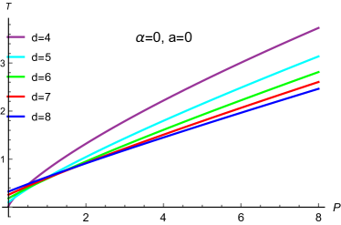
Fig. 3: The inversion curves versus $P$ for different dimensions. Here, we use $a=0$, $\alpha=0$ and $Q=1$.

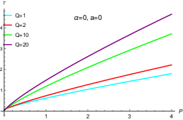
(a) $d=5$

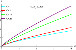
(b) $d=5$

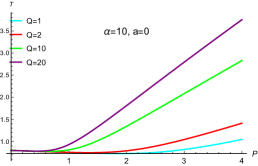
(c) $d=5$

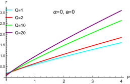
(d) $d=6$

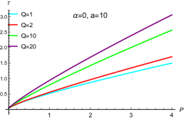
(e) $d=6$

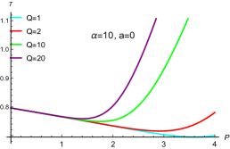
(f) $d=6$

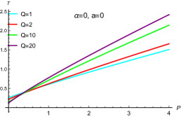
(g) $d=7$

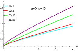
(h) $d=7$

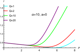
(i) $d=7$

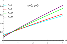
(j) $d=8$

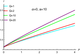
(k) $d=8$

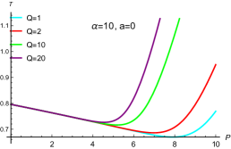
(l) $d=8$

Fig. 4: The inversion curves versus $P$ for various combinations of $d$, $a$, $\alpha$ and $Q$.

With the study of extending the black hole thermodynamics to the Joule-Thomson expansion regime, the inversion curves and the isenthalpic curves involved in the Joule-Thomson expansion of various black holes, have become major research interests. Besides, the results are often compared with van der Waals fluid. Here the investigation highlights the variations of the inversion curves concerning the parameters $d$, $a$, $\alpha$ and $Q$. As regards the derivation of the inversion temperature, we can obtain it from this approach by setting $\mu=0$, as follows

$$T_{i}=V(\frac{\partial T}{\partial V})_{P,Q,a,\alpha},$$ (20)

then, the inversion temperature for a d-dimensional charged AdS black hole with cloud of strings and quintessence is

$$T_{i}=\frac{2a(d-3)r_{+}^{4-d}+8(2d-5)\pi^{3-d}Q^{2}r_{+}^{6-2d}\Gamma\left(\frac{d-1}{2}\right)^{2}-(d-5)d+16\pi Pr_{+}^{2}-6}{4\pi(d-2)(d-1)r_{+}}.$$ (21)

In the case of $T_{i}=T=(\frac{\partial M}{\partial S})_{P,Q,a,\alpha}$, subtracting Eq. $\left(\ref{eqn:two11}\right)$ from Eq. $\left(\ref{eqn:fz3}\right)$ we can obtain

$$\frac{4ar_{+}^{3-d}+24\pi^{3-d}Q^{2}r_{+}^{5-2d}\Gamma\left(\frac{d-1}{2}\right)^{2}+\frac{(d-3)d\left(\alpha r_{+}-1\right)}{r_{+}}+2\left(\alpha-8\pi Pr_{+}\right)}{4\pi(d-1)}=0.$$ (22)

The explicit expressions for the inversion temperature can be obtained by substituting the roots into Eq. $\left(\ref{eqn:two11}\right)$, and the roots are obtained by solving Eq. $\left(\ref{eqn:fz4}\right)$. However, the explicit expressions for roots that satisfy the condition are so complicated that we do not represent them. In the following part of the paper, the numerical solution is the approach used to investigate.

In order to visualize how the inversion curve varies under the influence of $d$, Fig. 3 is shown with $Q$ fixed and without considering parameters $a$ and $\alpha$. As a result, the same observations as in literature Mo:2018rgq can be obtained, i.e., the effect of $d$ on the inversion curve is different in the high and low pressure cases. In the high-pressure case, the inversion curve decreases as $d$ increases, and the opposite is observed in the low-pressure case.

In Fig. 4, how parameters $Q$, $a$ and $\alpha$ affect the inversion curve are exhibited in the $T$-$P$ plane. By comparing the effect of Q on the inversion curve in different dimensions $d$ with $a$ and $\alpha$ fixed (e.g., comparing Figs. 4(a), 4(d), 4(g), 4(j)), it is evident that the inversion temperature for a given pressure increases with the increase of $Q$ in the high-pressure region and decreases with the increase of $Q$ in the low-pressure region. Note that this result is independent of $d$. Further, by comparing the influence of $a$ on the inversion curve in different dimensions, we can compare the first and second columns of the Fig. 4, for example, the comparison between Fig. 4(j) and Fig. 4(k). It can be seen that as $a$ changes the inversion curve also changes, whereby the high and low pressure dividing point becomes smaller as $a$ increases. Such a result holds in different dimensions $d$.

Observing the first and third columns of the figure, the change in $\alpha$ has changed the inversion curve significantly, i.e., the high and low pressure dividing points move to the right as $\alpha$ increases, moreover, the change is most pronounced in the low pressure region. Overall, the effect of $\alpha$ on the inversion curve is more profound than the effect of $a$ on the inversion curve. Combined with our findings in the literature Yin:2021akt regarding the four dimensions, it is known that the above mentioned conclusion is independent of $d$.

We next extend the study to cover the case of the isenthalpic curve.

III.3 The isenthalpic curve

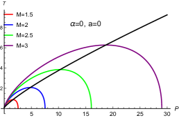
(a) $d=5$

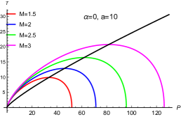
(b) $d=5$

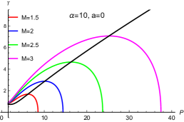
(c) $d=5$

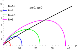
(d) $d=6$

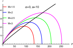
(e) $d=6$

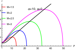
(f) $d=6$

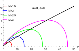
(g) $d=7$

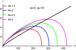
(h) $d=7$

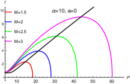
(i) $d=7$

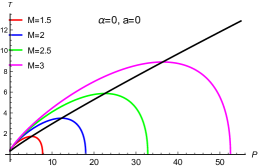
(j) $d=8$

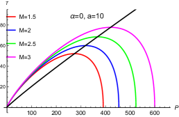
(k) $d=8$

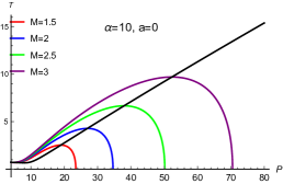
(l) $d=8$

Fig. 5: The isenthalpic curves and inversion curves for various combinations of $d$, $a$, $\alpha$ and $M$, with $Q$=1.

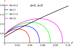
(a) $d=5$

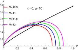
(b) $d=5$

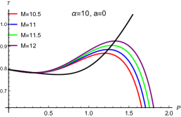
(c) $d=5$

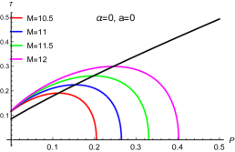
(d) $d=6$

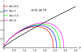
(e) $d=6$

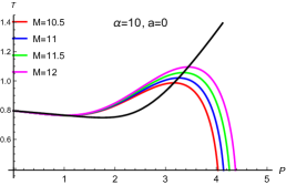
(f) $d=6$

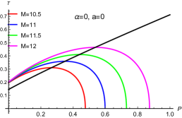
(g) $d=7$

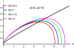
(h) $d=7$

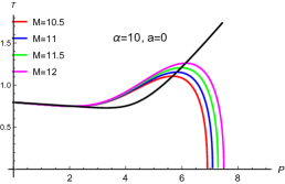
(i) $d=7$

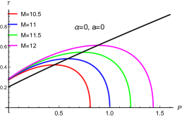
(j) $d=8$

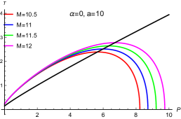
(k) $d=8$

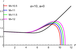
(l) $d=8$

Fig. 6: The isenthalpic curves and inversion curves for various combinations of $d$, $a$, $\alpha$ and $M$, here $Q$=10.

In the process of studying the Joule-Thomson expansion of d-dimensional charged AdS black holes with cloud of strings and quintessence, it is necessary to analyze the changes in the isenthalpic curves under the influence of different parameters. Specifically, the main purpose of this section is to disclose the fine structure of the isenthalpic curves in the case of parameters $a$, $\alpha$ and $d$ change. The solution can be solved for Eq. $\left(\ref{eqn:two6}\right)$ with a given value of $M$, and then substituting the solution into Eq. $\left(\ref{eqn:two11}\right)$ we can obtain the isenthalpic temperature. Note that $M>Q$, which is chosen to ensure that it does not appear in the $T-P$ plane as a particular hypersurfaces with naked singularity Okcu:2016tgt ; Ghaffarnejad:2013cma . The specific expressions of the solutions are not listed here.

For further study, the isenthalpic curves and the inversion curves are plotted simultaneously in Fig. 5 and Fig. 6 under the different parameters. As can be seen from the two figures above, both the isenthalpic curves and the inversion curves are present under the situation ($M>Q$), which shows the occurrence of the Joule-Thomson expansion. By careful observation, it is found that with $Q$ kept constant, the inversion curves all coincide with the highest point of the isenthalpic curves, and the isenthalpic curves is divided into two regions by the inversion curves. In the region above the inversion curves, the slope of the isenthalpic curves is positive, which means that cooling occurs. In the region below the inversion curves, the slope of the isenthalpic curves is negative, when heating occurs. So the inversion curves is the dividing line between the cooling and heating regions of the isenthalpic curves. By comparing Fig. 5 and Fig. 6, it is evident that as $Q$ increases, the cooling-heating critical point changes and the curves tends to move to the left, which is independent of the parameters $a$, $\alpha$ and $d$. When only the effect of $M$ on the isenthalpic curve is considered, it can be seen that as $M$ increases, the curve expands to the right, correspondingly, the cooling-heating critical point also increases.

From the first and second columns of Figs. 5 and 6, we can have the impression that the isenthalpic curves changes as $a$ increases, i.e., the curve tends to expand to the right, when other conditions remain constant. A similar changes in parameters $d$ and $\alpha$ are found by comparison. As $d$ increases, the curves tend to expand at higher pressures, which is independent of the other parameters and is consistent with the findings in the literature Yin:2021akt . Comparing the first column and the third column of the two graphs, one difference is that when $\alpha$ changes, the slope variation of the isenthalpic curve may be somewhat different in the cooling region.

III.4 The ratio between $T_{i}^{min}$ and $T_{c}$

This section focuses on criticality. The first step is to find the stationary inflection points in $P(r_{+})-r_{+}$ diagram. The equation of state $P=P(V,T)$ for the black hole is obtained from Eq. $\left(\ref{eqn:two11}\right)$ as

$$P=\frac{2ar_{+}^{4-d}+8\pi^{3-d}Q^{2}\Gamma\left(\frac{d-1}{2}\right)^{2}r_{+}^{6-2d}+(d-2)\left(\alpha(d-2)r_{+}-d+4\pi Tr_{+}+3\right)}{16\pi r_{+}^{2}},$$ (23)

then, the critical point can be obtained using the following conditions Kubiznak:2012wp

$$\frac{\partial P}{\partial r_{+}}=0,\frac{\partial^{2}P}{\partial r_{+}^{2}}=0.$$ (24)

Since the explicit expressions for the solution is too long to be easily expressed, the results for the critical values will be given in the Table 1 for diverse cases. It is observed that, when $d=4$, the results for critical point are consistent with the correlation results derived in the Ref. Chabab:2020ejk . Next, numerical calculations are performed for further study, and for the case of $Q=1$, we present the results in Table 2, Table 3, Table 4, Table 5 and Table 6.

Noting that $T_{i}^{min}$ can be obtained by demanding $P_{i}=0$, while $P_{i}$ can be derived from $\mu=0$. After setting $\mu=0$ and substituting $P_{i}=0$ into Eq. $\left(\ref{eqn:J8}\right)$, the following expression regarding $T_{i}^{min}$ can be obtained

$$\frac{4r_{\min}\left(\frac{4\pi^{d-1}r_{\min}^{d+\frac{8}{d-1}+2}\left(4ar_{\min}^{4}+r_{\min}^{d}\left((d-3)d\left(\alpha r_{\min}-1\right)+2\alpha r_{\min}\right)\right)}{\Gamma\left(\frac{d-1}{2}\right)^{2}}+96\pi^{2}Q^{2}r_{\min}^{\frac{8d}{d-1}}\right)}{(d-1)\left(\frac{4\pi^{d-1}r_{\min}^{d+\frac{8}{d-1}+2}\left(2ar_{\min}^{4}+(d-2)r_{\min}^{d}\left(\alpha(d-2)r_{\min}-d+3\right)\right)}{\Gamma\left(\frac{d-1}{2}\right)^{2}}+32\pi^{2}Q^{2}r_{\min}^{\frac{8d}{d-1}}\right)}=0,$$ (25)

and

$$T_{i}^{min}=-\frac{\frac{2ar_{min}^{4-d}}{d-2}+\frac{8\pi^{3-d}Q^{2}r_{min}^{6-2d}\Gamma\left(\frac{d-1}{2}\right)^{2}}{d-2}+\alpha(d-2)r_{min}-d+3}{4\pi r_{min}}.$$ (26)

The Tables 7, 8, 9, 10 and 11 are listed by fixing the values of any two parameters of $d$, $a$ and $\alpha$ while changing the value of the other parameter in the case of $Q=1$. The final Table 12 is obtained after integration of data.

It can be observed that when the dimension is fixed, the change of $r_{c}$ is mainly related to $a$. The reason is that only $a$ but not $\alpha$ exists in the expression about $r_{c}$. For the same reason, the variation of $P_{c}$ is also mainly related to $a$. $r_{c}$ and $P_{c}$ decrease with the increase of $a$. It is obvious that $T_{c}$ decreases with the increase of $a$ or $\alpha$. Then we concentrate on observing the effect of dimension $d$. With Tables 2, 3, 4,5, and 6, it can be found that as $d$ increases, $r_{c}$ decreases, $P_{c}$ increases, and $T_{c}$ also increases.

By observing Tables 7, 8, 9, 10 and 11, changes in $d$, $a$ and $\alpha$ can also have a visible effect on $r_{min}$ and $T_{i}^{min}$. The increase of $d$, $a$ and $\alpha$ will all increase $r_{min}$ as well. $T_{i}^{min}$ increases as $d$ increases, however the increase in $a$ and $\alpha$ causes $T_{i}^{min}$ to decrease. The analysis of the ratio of $T_{c}$ and $T_{i}^{min}$ in relation to the above observation continues as shown in the Table 12. The ratio $\frac{T_{i}^{min}}{T_{c}}$ decreases with the increase of both dimension $d$ and parameter of quintessence $\alpha$. The difference is that the ratio $\frac{T_{i}^{min}}{T_{c}}$ increases with the increase of parameter of cloud of strings $a$. It is worth of attention that the ratios are all less than 1/2 and converge to 1/2, independently of $d$, $a$ and $\alpha$. It proves that the ratio turned out to be 1/2 is not a universal phenomenon but mainly exists in four-dimensional spacetime.

Table 1: The critical physical quantities ($r_{c}$, $P_{c}$ and $T_{c}$) for various dimensions.

$d$	$r_{c}$	$P_{c}$	$T_{c}$
4	$\frac{\sqrt{6}Q}{\sqrt{1-a}}$	$\frac{(a-1)^{2}}{96\pi Q^{2}}$	$\frac{\sqrt{6}\text{(}1-a)^{\frac{3}{2}}-9\alpha Q}{18\pi Q}$
5	$\frac{3r_{c}^{3}(a-r_{c})+\frac{60Q^{2}}{\pi^{2}}}{4\pi r_{c}^{8}}=0$	$\frac{\pi^{2}r_{c}^{3}\left(3r_{c}-2a\right)-20Q^{2}}{8\pi^{3}r_{c}^{6}}$	$\frac{\pi^{2}r_{c}^{3}\left(r_{c}\left(4-3\alpha r_{c}\right)-2a\right)-16Q^{2}}{4\pi^{3}r_{c}^{5}}$
6	$\frac{6\pi^{2}r_{c}^{4}\left(a-r_{c}^{2}\right)+63Q^{2}}{4\pi^{3}r_{c}^{10}}=0$	$-\frac{3\left(4\pi^{2}r_{c}^{4}\left(a-2r_{c}^{2}\right)+21Q^{2}\right)}{32\pi^{3}r_{c}^{8}}$	$-\frac{2\pi^{2}r_{c}^{4}\left(a+r_{c}^{2}\left(2\alpha r_{c}-3\right)\right)+9Q^{2}}{4\pi^{3}r_{c}^{7}}$
7	$\frac{5\left(\pi^{4}r_{c}^{5}\left(a-r_{c}^{3}\right)+72Q^{2}\right)}{2\pi^{5}r_{c}^{12}}=0$	$\frac{\pi^{4}r_{c}^{5}\left(5r_{c}^{3}-2a\right)-72Q^{2}}{4\pi^{5}r_{c}^{10}}$	$-\frac{\pi^{4}r_{c}^{5}\left(2a+r_{c}^{3}\left(5\alpha r_{c}-8\right)\right)+64Q^{2}}{4\pi^{5}r_{c}^{9}}$
8	$\frac{15\left(8\pi^{4}r_{c}^{6}\left(a-r_{c}^{4}\right)+495Q^{2}\right)}{32\pi^{5}r_{c}^{14}}=0$	$-\frac{5\left(16\pi^{4}r_{c}^{6}\left(a-3r_{c}^{4}\right)+495Q^{2}\right)}{128\pi^{5}r_{c}^{12}}$	$-\frac{8\pi^{4}r_{c}^{6}\left(a+r_{c}^{4}\left(3\alpha r_{c}-5\right)\right)+225Q^{2}}{16\pi^{5}r_{c}^{11}}$

Table 2: The critical physical quantities ($r_{c}$, $P_{c}$ and $T_{c}$) for $d=4$.

$d=4$	$r_{c}$	$P_{c}$	$T_{c}$
$a=0,\alpha=0$	2.44949	0.003316	0.043317
$a=0,\alpha=0.05$	2.44949	0.003316	0.035359
$a=0.5,\alpha=0$	3.4641	0.000829	0.015315
$a=0.5,\alpha=0.05$	3.4641	0.000829	0.007357

Table 3: The critical physical quantities ($r_{c}$, $P_{c}$ and $T_{c}$) for $d=5$.

$d=5$	$r_{c}$	$P_{c}$	$T_{c}$
$a=0,\alpha=0$	1.19312	0.055902	0.213431
$a=0,\alpha=0.05$	1.19312	0.055902	0.201494
$a=0.5,\alpha=0$	1.34076	0.036013	0.163367
$a=0.5,\alpha=0.05$	1.34076	0.036013	0.15143

Table 4: The critical physical quantities ($r_{c}$, $P_{c}$ and $T_{c}$) for $d=6$.

$d=6$	$r_{c}$	$P_{c}$	$T_{c}$
$a=0,\alpha=0$	1.01037	0.175392	0.405054
$a=0,\alpha=0.05$	1.01037	0.175392	0.389139
$a=0.5,\alpha=0$	1.10345	0.126923	0.337043
$a=0.5,\alpha=0.05$	1.10345	0.126923	0.321127

Table 5: The critical physical quantities ($r_{c}$, $P_{c}$ and $T_{c}$) for $d=7$.

$d=7$	$r_{c}$	$P_{c}$	$T_{c}$
$a=0,\alpha=0$	0.962923	0.343295	0.587673
$a=0,\alpha=0.05$	0.962923	0.343295	0.567779
$a=0.5,\alpha=0$	1.0372	0.262741	0.50739
$a=0.5,\alpha=0.05$	1.0372	0.262741	0.487495

Table 6: The critical physical quantities ($r_{c}$, $P_{c}$ and $T_{c}$) for $d=8$.

$d=8$	$r_{c}$	$P_{c}$	$T_{c}$
$a=0,\alpha=0$	0.955634	0.544612	0.757017
$a=0,\alpha=0.05$	0.955634	0.544612	0.733144
$a=0.5,\alpha=0$	1.01757	0.435529	0.671153
$a=0.5,\alpha=0.05$	1.01757	0.435529	0.64728

Table 7: The minimum inversion temperature ($T_{i}^{min}$) and its corresponding root ($r_{min}$) for $d=4$.

$d=4$	$r_{min}$	$T_{i}^{min}$
$a=0,\alpha=0$	1.22474	0.021658
$a=0,\alpha=0.05$	1.28859	0.016606
$a=0.5,\alpha=0$	1.73205	0.007657
$a=0.5,\alpha=0.05$	2.09059	0.002365

Table 8: The minimum inversion temperature ($T_{i}^{min}$) and its corresponding root ($r_{min}$) for $d=5$.

$d=5$	$r_{min}$	$T_{i}^{min}$
$a=0,\alpha=0$	0.702228	0.10073
$a=0,\alpha=0.05$	0.709911	0.093009
$a=0.5,\alpha=0$	0.758108	0.077921
$a=0.5,\alpha=0.05$	0.769404	0.070368

Table 9: The minimum inversion temperature ($T_{i}^{min}$) and its corresponding root ($r_{min}$) for $d=6$.

$d=6$	$r_{min}$	$T_{i}^{min}$
$a=0,\alpha=0$	0.650819	0.183409
$a=0,\alpha=0.05$	0.654851	0.172996
$a=0.5,\alpha=0$	0.681196	0.1542511
$a=0.5,\alpha=0.05$	0.686482	0.144099

Table 10: The minimum inversion temperature ($T_{i}^{min}$) and its corresponding root ($r_{min}$) for $d=7$.

$d=7$	$r_{min}$	$T_{i}^{min}$
$a=0,\alpha=0$	0.658134	0.257949
$a=0,\alpha=0.05$	0.661107	0.244853
$a=0.5,\alpha=0$	0.6797104	0.224907
$a=0.5,\alpha=0.05$	0.683421	0.212149

Table 11: The minimum inversion temperature ($T_{i}^{min}$) and its corresponding root ($r_{min}$) for $d=8$.

$d=8$	$r_{min}$	$T_{i}^{min}$
$a=0,\alpha=0$	0.681641	0.324289
$a=0,\alpha=0.05$	0.684138	0.308516
$a=0.5,\alpha=0$	0.69796	0.290015
$a=0.5,\alpha=0.05$	0.700967	0.274635

Table 12: The ratio $\frac{T_{i}^{min}}{T_{c}}$ for various combinations of $d$, $a$ and $\alpha$.

$\frac{T_{i}^{min}}{T_{c}}$
	$a=0,\alpha=0$	$a=0,\alpha=0.05$	$a=0.5,\alpha=0$	$a=0.5,\alpha=0.05$
$d=4$	0.499999	0.46965	0.5	0.321498
$d=5$	0.471956	0.461594	0.476968	0.464689
$d=6$	0.452801	0.444561	0.45766	0.448729
$d=7$	0.438933	0.431247	0.443263	0.435182
$d=8$	0.428377	0.420812	0.432115	0.424291

IV Conclusion and Discussion

This paper investigated the Joule-Thomson expansion of the charged AdS black hole with cloud of strings and quintessence, which present in higher dimensional spacetime. In extended phase space, the mass of the black hole is interpreted as enthalpy, while the cosmological constant is treated as thermodynamic pressure. After a brief review of the thermodynamics of the black hole, the Joule-Thomson expansion effect of the black hole was discussed in detail from four aspects: the Joule-Thomson coefficient, the inversion curve, the isenthalpic curve and the ratio between $T_{i}^{min}$ and $T_{c}$. At the extreme values of the isenthalpic curve, the Joule-Thomson coefficient is exactly zero, and the trajectories of these points are described as inversion curve.

The Joule-Thomson effect is an irreversible adiabatic expansion, in which temperature changes with pressure and enthalpy are constant. And the variation between temperature and pressure determines the sign of the Joule-Thomson coefficient. We plotted Fig. 1 and Fig. 2 to visualize this variation when setting $P$ certain. It turns out that the existence of divergence point dividing the Joule-Thomson coefficient curve into positive and negative infinity regions, and the divergence point of Joule-Thomson coefficient corresponds to the zero point of Hawking temperature. Further, as $d$, $q$, $a$ and $\alpha$ increase, the divergence point moves to the right.

Then we investigated the inversion curve with the approach of numerical analysis. Different figures exhibit that the inversion curves change with the parameters $d$, $Q$, $a$ and $\alpha$ for each plot. The specific variations are presented in detail in the Table 13.

Table 13: Findings for the effects of different parameters on the inversion curves.

parameters	The effects of parameters on the inversion curves
$d$	In the high-pressure case, the inversion temperature for a given pressure decreases as $d$ increases; In the low-pressure case, the inversion temperature for a given pressure increases as $d$ increases.
$Q$	In the high-pressure region, the inversion temperature for a given pressure increases with the increase of $Q$; In the low-pressure region, the inversion temperature for a given pressure decreases with the increase of $Q$.
$a$	The high and low pressure dividing points move to the left as $a$ increases.
$\alpha$	The high and low pressure dividing points move to the right as $\alpha$ increases. The change is most pronounced in the low pressure region.

And thirdly, under the premise of $M>Q$, we studied the variations of the isenthalpic curve in the $T$ - $P$ plane. When combined with the inversion curve, it shows that the Joule-Thomson expansion is present in all states. Meanwhile, The inversion curve passes through the maximum point of the isenthalpic curve, thus dividing the isenthalpic curve into two regions: heating (one occurs in the region below the inversion curves) and cooling (one occurs in the region above the inversion curves). Different figures exhibit that the isenthalpic curves change with the parameters $d$, $Q$, $M$, $a$ and $\alpha$ for each plot. The specific findings are presented in detail in the Table 14.

Table 14: Findings for the effects of different parameters on the isenthalpic curves.

parameters	The effects of parameters on the isenthalpic curves
$d$	As $d$ increases, the cooling-heating critical points change, the curves tend to expand at higher pressures.
$M$	As $M$ increases, the cooling-heating critical points increase, and the curves expand to the right.
$Q$	As $Q$ increases, the cooling-heating critical points change and the curves tend to move to the left
$a$	As $a$ increases, the cooling-heating critical points change, the curves tend to expand to the right.
$\alpha$	As $\alpha$ increases, the cooling-heating critical points change, the curves tend to expand to the right. Note that in the cooling region, when the value of $\alpha$ changes, the slope of the isoenthalpy curve changes as well.

Furthermore, the critical quantities such as $r_{c}$, $P_{c}$ and $T_{c}$ were studied, where the ratio between $T_{i}^{min}$ and $T_{c}$ was the focus of the analysis. The results of the critical quantities in different dimensions are summarized in the Table 1. It is found that even though some of the critical quantities are difficult to obtain specific expressions, the critical values all change independently of the parameter $\alpha$. This conclusion is also verified by the method of numerical calculations we subsequently employed. Next we analyzed the effects of different parameters $d$, $a$ and $\alpha$ on critical quantities, minimum inversion temperatures, and ratios, which are presented in the Table 15.

Table 15: Findings for the effects of different parameters on critical quantities, minimum inversion temperatures, and ratios.

	$d$	$a$	$\alpha$
$r_{c}$	As $d$ increases, $r_{c}$ decreases.	As $a$ increases, $r_{c}$ increases.	$\alpha$ has no effect on $r_{c}$.
$P_{c}$	As $d$ increases, $P_{c}$ increases.	As $a$ increases, $P_{c}$ decreases	$\alpha$ has no effect on $P_{c}$.
$T_{c}$	As $d$ increases, $T_{c}$ increases.	As $a$ increases, $T_{c}$ decreases	As $\alpha$ increases, $T_{c}$ decreases
$r_{min}$	As $d$ increases, $r_{min}$ increases.	As $a$ increases, $r_{min}$ increases	As $\alpha$ increases, $r_{min}$ increases
$T_{i}^{min}$	As $d$ increases, $T_{i}^{min}$ increases	As $a$ increases, $T_{i}^{min}$ decreases	As $\alpha$ increases, $T_{i}^{min}$ decreases
$\frac{T_{i}^{min}}{T_{c}}$	As $d$ increases, $\frac{T_{i}^{min}}{T_{c}}$ decreases.	As $a$ increases, $\frac{T_{i}^{min}}{T_{c}}$ increases.	As $\alpha$ increases, $\frac{T_{i}^{min}}{T_{c}}$ decreases.

- (1) J. D. Bekenstein, “Black holes and the second law,” Lett. Nuovo Cim. 4, 737-740 (1972) doi:10.1007/BF02757029
- (2) J. M. Bardeen, B. Carter and S. W. Hawking, “The Four laws of black hole mechanics,” Commun. Math. Phys. 31, 161-170 (1973) doi:10.1007/BF01645742
- (3) S. W. Hawking, “Black hole explosions,” Nature 248, 30-31 (1974) doi:10.1038/248030a0
- (4) S. W. Hawking, “Particle Creation by Black Holes,” Commun. Math. Phys. 43, 199-220 (1975) [erratum: Commun. Math. Phys. 46, 206 (1976)] doi:10.1007/BF02345020
- (5) S. W. Hawking, “Black Holes and Thermodynamics,” Phys. Rev. D 13, 191-197 (1976) doi:10.1103/PhysRevD.13.191
- (6) S. Perlmutter et al. [Supernova Cosmology Project], “Measurements of and from 42 high redshift supernovae,” Astrophys. J. 517, 565-586 (1999) doi:10.1086/307221 [arXiv:astro-ph/9812133 [astro-ph]].
- (7) P. M. Garnavich et al. [Supernova Search Team], “Supernova limits on the cosmic equation of state,” Astrophys. J. 509, 74-79 (1998) doi:10.1086/306495 [arXiv:astro-ph/9806396 [astro-ph]].
- (8) B. Ratra and P. J. E. Peebles, “Cosmological Consequences of a Rolling Homogeneous Scalar Field,” Phys. Rev. D 37, 3406 (1988) doi:10.1103/PhysRevD.37.3406
- (9) R. R. Caldwell, R. Dave and P. J. Steinhardt, “Cosmological imprint of an energy component with general equation of state,” Phys. Rev. Lett. 80, 1582-1585 (1998) doi:10.1103/PhysRevLett.80.1582 [arXiv:astro-ph/9708069 [astro-ph]].
- (10) V. V. Kiselev, “Quintessence and black holes,” Class. Quant. Grav. 20, 1187-1198 (2003) doi:10.1088/0264-9381/20/6/310 [arXiv:gr-qc/0210040 [gr-qc]].
- (11) S. Chen, B. Wang and R. Su, “Hawking radiation in a -dimensional static spherically-symmetric black Hole surrounded by quintessence,” Phys. Rev. D 77, 124011 (2008) doi:10.1103/PhysRevD.77.124011 [arXiv:0801.2053 [gr-qc]].
- (12) M. Azreg-Aïnou, “Charged de Sitter-like black holes: quintessence-dependent enthalpy and new extreme solutions,” Eur. Phys. J. C 75, no.1, 34 (2015) doi:10.1140/epjc/s10052-015-3258-3 [arXiv:1410.1737 [gr-qc]].
- (13) S. G. Ghosh, M. Amir and S. D. Maharaj, “Quintessence background for 5D Einstein–Gauss–Bonnet black holes,” Eur. Phys. J. C 77, no.8, 530 (2017) doi:10.1140/epjc/s10052-017-5099-8 [arXiv:1611.02936 [gr-qc]].
- (14) S. G. Ghosh, S. D. Maharaj, D. Baboolal and T. H. Lee, “Lovelock black holes surrounded by quintessence,” Eur. Phys. J. C 78, no.2, 90 (2018) doi:10.1140/epjc/s10052-018-5570-1 [arXiv:1708.03884 [gr-qc]].
- (15) S. H. Henry Tye, “Brane inflation: String theory viewed from the cosmos,” Lect. Notes Phys. 737, 949-974 (2008) [arXiv:hep-th/0610221 [hep-th]].
- (16) P. S. Letelier, “CLOUDS OF STRINGS IN GENERAL RELATIVITY,” Phys. Rev. D 20, 1294-1302 (1979) doi:10.1103/PhysRevD.20.1294
- (17) S. G. Ghosh, U. Papnoi and S. D. Maharaj, “Cloud of strings in third order Lovelock gravity,” Phys. Rev. D 90, no.4, 044068 (2014) doi:10.1103/PhysRevD.90.044068 [arXiv:1408.4611 [gr-qc]].
- (18) E. Herscovich and M. G. Richarte, “Black holes in Einstein-Gauss-Bonnet gravity with a string cloud background,” Phys. Lett. B 689, 192-200 (2010) doi:10.1016/j.physletb.2010.04.065 [arXiv:1004.3754 [hep-th]].
- (19) M. G. Richarte and C. Simeone, “Traversable wormholes in a string cloud,” Int. J. Mod. Phys. D 17, 1179-1196 (2008) doi:10.1142/S0218271808012759 [arXiv:0711.2297 [gr-qc]].
- (20) A. K. Yadav, V. K. Yadav and L. Yadav, “Cylindrically symmetric inhomogeneous universes with a cloud of strings,” Int. J. Theor. Phys. 48, 568-578 (2009) doi:10.1007/s10773-008-9832-9 [arXiv:1112.4114 [gr-qc]].
- (21) A. Ganguly, S. G. Ghosh and S. D. Maharaj, “Accretion onto a black hole in a string cloud background,” Phys. Rev. D 90, no.6, 064037 (2014) doi:10.1103/PhysRevD.90.064037 [arXiv:1409.7872 [gr-qc]].
- (22) K. A. Bronnikov, S. W. Kim and M. V. Skvortsova, “The Birkhohff theorem and string clouds,” Class. Quant. Grav. 33, no.19, 195006 (2016) doi:10.1088/0264-9381/33/19/195006 [arXiv:1604.04905 [gr-qc]].
- (23) S. G. Ghosh and S. D. Maharaj, “Cloud of strings for radiating black holes in Lovelock gravity,” Phys. Rev. D 89, no.8, 084027 (2014) doi:10.1103/PhysRevD.89.084027 [arXiv:1409.7874 [gr-qc]].
- (24) T. H. Lee, D. Baboolal and S. G. Ghosh, “Lovelock black holes in a string cloud background,” Eur. Phys. J. C 75, no.7, 297 (2015) doi:10.1140/epjc/s10052-015-3515-5 [arXiv:1409.2615 [gr-qc]].
- (25) M. K. Parikh and F. Wilczek, “Hawking radiation as tunneling,” Phys. Rev. Lett. 85, 5042-5045 (2000) doi:10.1103/PhysRevLett.85.5042 [arXiv:hep-th/9907001 [hep-th]].
- (26) R. Kerner and R. B. Mann, “Fermions tunnelling from black holes,” Class. Quant. Grav. 25, 095014 (2008) doi:10.1088/0264-9381/25/9/095014 [arXiv:0710.0612 [hep-th]].
- (27) Z. W. Feng, H. L. Li, X. T. Zu and S. Z. Yang, “Corrections to the thermodynamics of Schwarzschild-Tangherlini black hole and the generalized uncertainty principle,” Eur. Phys. J. C 76, no.4, 212 (2016) doi:10.1140/epjc/s10052-016-4057-1 [arXiv:1604.04702 [hep-th]].
- (28) S. Hod, “A lower bound on the Bekenstein-Hawking temperature of black holes,” Phys. Lett. B 759, 541 (2016) doi:10.1016/j.physletb.2016.06.021 [arXiv:1701.00492 [gr-qc]].
- (29) J. R. Muñoz de Nova, K. Golubkov, V. I. Kolobov and J. Steinhauer, “Observation of thermal Hawking radiation and its temperature in an analogue black hole,” Nature 569, no.7758, 688-691 (2019) doi:10.1038/s41586-019-1241-0 [arXiv:1809.00913 [gr-qc]].
- (30) C. W. Robson, L. Di Mauro Villari and F. Biancalana, “Topological nature of the Hawking temperature of black holes,” Phys. Rev. D 99, no.4, 044042 (2019) doi:10.1103/PhysRevD.99.044042 [arXiv:1810.09322 [gr-qc]].
- (31) Z. W. Feng, Q. C. Ding and S. Z. Yang, “Modified fermion tunneling from higher-dimensional charged AdS black hole in massive gravity,” Eur. Phys. J. C 79, no.5, 445 (2019) doi:10.1140/epjc/s10052-019-6959-1 [arXiv:1810.05645 [gr-qc]].
- (32) A. Moreno-Ruiz and D. Bermudez, “Hawking temperature in dispersive media: Analytics and numerics,” Annals Phys. 420, 168268 (2020) doi:10.1016/j.aop.2020.168268 [arXiv:1908.02368 [gr-qc]].
- (33) S. W. Hawking and D. N. Page, “Thermodynamics of Black Holes in anti-De Sitter Space,” Commun. Math. Phys. 87, 577 (1983) doi:10.1007/BF01208266
- (34) A. Chamblin, R. Emparan, C. V. Johnson and R. C. Myers, “Charged AdS black holes and catastrophic holography,” Phys. Rev. D 60, 064018 (1999) doi:10.1103/PhysRevD.60.064018 [arXiv:hep-th/9902170 [hep-th]].
- (35) A. Chamblin, R. Emparan, C. V. Johnson and R. C. Myers, “Holography, thermodynamics and fluctuations of charged AdS black holes,” Phys. Rev. D 60, 104026 (1999) doi:10.1103/PhysRevD.60.104026 [arXiv:hep-th/9904197 [hep-th]].
- (36) S. W. Wei, Q. T. Man and H. Yu, “Thermodynamic Geometry of Charged AdS Black Hole Surrounded by Quintessence,” Commun. Theor. Phys. 69, no.2, 173 (2018) doi:10.1088/0253-6102/69/2/173
- (37) R. Banerjee and D. Roychowdhury, “Thermodynamics of phase transition in higher dimensional AdS black holes,” JHEP 11, 004 (2011) doi:10.1007/JHEP11(2011)004 [arXiv:1109.2433 [gr-qc]].
- (38) M. M. Caldarelli, G. Cognola and D. Klemm, “Thermodynamics of Kerr-Newman-AdS black holes and conformal field theories,” Class. Quant. Grav. 17, 399-420 (2000) doi:10.1088/0264-9381/17/2/310 [arXiv:hep-th/9908022 [hep-th]].
- (39) D. Kastor, S. Ray and J. Traschen, “Enthalpy and the Mechanics of AdS Black Holes,” Class. Quant. Grav. 26, 195011 (2009) doi:10.1088/0264-9381/26/19/195011 [arXiv:0904.2765 [hep-th]].
- (40) D. Kastor, S. Ray and J. Traschen, “Smarr Formula and an Extended First Law for Lovelock Gravity,” Class. Quant. Grav. 27, 235014 (2010) doi:10.1088/0264-9381/27/23/235014 [arXiv:1005.5053 [hep-th]].
- (41) B. P. Dolan, “The cosmological constant and the black hole equation of state,” Class. Quant. Grav. 28, 125020 (2011) doi:10.1088/0264-9381/28/12/125020 [arXiv:1008.5023 [gr-qc]].
- (42) B. P. Dolan, “Pressure and volume in the first law of black hole thermodynamics,” Class. Quant. Grav. 28, 235017 (2011) doi:10.1088/0264-9381/28/23/235017 [arXiv:1106.6260 [gr-qc]].
- (43) M. Cvetic, G. W. Gibbons, D. Kubiznak and C. N. Pope, “Black Hole Enthalpy and an Entropy Inequality for the Thermodynamic Volume,” Phys. Rev. D 84, 024037 (2011) doi:10.1103/PhysRevD.84.024037 [arXiv:1012.2888 [hep-th]].
- (44) R. Yin, J. Liang and B. Mu, “Stability of horizon with pressure and volume of d-dimensional charged AdS black holes with cloud of strings and quintessence,” Phys. Dark Univ. 32, 100831 (2021) doi:10.1016/j.dark.2021.100831 [arXiv:2103.08162 [gr-qc]].
- (45) B. Mu, J. Liang and X. Guo, “Thermodynamics with pressure and volume of black holes based on two assumptions under scalar field scattering,” [arXiv:2101.11414 [gr-qc]].
- (46) H. Jing, B. Mu, J. Tao and P. Wang, “Thermodynamic instability of 3D Einstein-Born-Infeld AdS black holes,” Chin. Phys. C 45, no.6, 065103 (2021) doi:10.1088/1674-1137/abf1dc [arXiv:2012.14206 [gr-qc]].
- (47) B. Mu, J. Liang and X. Guo, “Thermodynamics with pressure and volume of 4D Gauss-Bonnet AdS Black Holes under the scalar field,” [arXiv:2011.00273 [gr-qc]].
- (48) J. Liang, B. Mu and J. Tao, “Thermodynamics and overcharging problem in the extended phase spaces of charged AdS black holes with cloud of strings and quintessence under charged particle absorption,” Chin. Phys. C 45, no.2, 023121 (2021) doi:10.1088/1674-1137/abd085 [arXiv:2008.09512 [gr-qc]].
- (49) J. Liang, X. Guo, D. Chen and B. Mu, “Remarks on the weak cosmic censorship conjecture of RN-AdS black holes with cloud of strings and quintessence under the scalar field,” Nucl. Phys. B 965, 115335 (2021) doi:10.1016/j.nuclphysb.2021.115335 [arXiv:2008.08327 [gr-qc]].
- (50) W. Hong, B. Mu and J. Tao, “Thermodynamics and weak cosmic censorship conjecture in the charged RN-AdS black hole surrounded by quintessence under the scalar field,” Nucl. Phys. B 949, 114826 (2019) doi:10.1016/j.nuclphysb.2019.114826 [arXiv:1905.07747 [gr-qc]].
- (51) Ö. Ökcü and E. Aydıner, “Joule–Thomson expansion of the charged AdS black holes,” Eur. Phys. J. C 77, no.1, 24 (2017) doi:10.1140/epjc/s10052-017-4598-y [arXiv:1611.06327 [gr-qc]].
- (52) Ö. Ökcü and E. Aydıner, “Joule–Thomson expansion of Kerr–AdS black holes,” Eur. Phys. J. C 78, no.2, 123 (2018) doi:10.1140/epjc/s10052-018-5602-x [arXiv:1709.06426 [gr-qc]].
- (53) A. Rizwan C.L., N. Kumara A., D. Vaid and K. M. Ajith, “Joule-Thomson expansion in AdS black hole with a global monopole,” Int. J. Mod. Phys. A 33, no.35, 1850210 (2019) doi:10.1142/S0217751X1850210X [arXiv:1805.11053 [gr-qc]].
- (54) J. X. Mo and G. Q. Li, “Effects of Lovelock gravity on the Joule–Thomson expansion,” Class. Quant. Grav. 37, no.4, 045009 (2020) doi:10.1088/1361-6382/ab60b9 [arXiv:1805.04327 [gr-qc]].
- (55) S. Q. Lan, “Joule-Thomson expansion of charged Gauss-Bonnet black holes in AdS space,” Phys. Rev. D 98, no.8, 084014 (2018) doi:10.1103/PhysRevD.98.084014 [arXiv:1805.05817 [gr-qc]].
- (56) J. X. Mo, G. Q. Li, S. Q. Lan and X. B. Xu, “Joule-Thomson expansion of -dimensional charged AdS black holes,” Phys. Rev. D 98, no.12, 124032 (2018) doi:10.1103/PhysRevD.98.124032 [arXiv:1804.02650 [gr-qc]].
- (57) H. Ghaffarnejad, E. Yaraie and M. Farsam, “Quintessence Reissner Nordström Anti de Sitter Black Holes and Joule Thomson effect,” Int. J. Theor. Phys. 57, no.6, 1671-1682 (2018) doi:10.1007/s10773-018-3693-7 [arXiv:1802.08749 [gr-qc]].
- (58) R. D’Almeida and K. P. Yogendran, “Thermodynamic Properties of Holographic superfluids,” [arXiv:1802.05116 [hep-th]].
- (59) M. Chabab, H. El Moumni, S. Iraoui, K. Masmar and S. Zhizeh, “Joule-Thomson Expansion of RN-AdS Black Holes in gravity,” LHEP 02, 05 (2018) doi:10.31526/LHEP.2.2018.02 [arXiv:1804.10042 [gr-qc]].
- (60) J. Liang, W. Lin and B. Mu, “Joule–Thomson expansion of the torus-like black hole,” Eur. Phys. J. Plus 136, no.11, 1169 (2021) doi:10.1140/epjp/s13360-021-02119-y [arXiv:2103.03119 [gr-qc]].
- (61) K. Hegde, A. Naveena Kumara, C. L. A. Rizwan, A. K. M. and M. S. Ali, “Thermodynamics, Phase Transition and Joule Thomson Expansion of novel 4-D Gauss Bonnet AdS Black Hole,” [arXiv:2003.08778 [gr-qc]].
- (62) S. W. Wei and Y. X. Liu, “Charged AdS black hole heat engines,” Nucl. Phys. B, 114700 (2019) doi:10.1016/j.nuclphysb.2019.114700 [arXiv:1708.08176 [gr-qc]].
- (63) X. M. Kuang, B. Liu and A. Övgün, “Nonlinear electrodynamics AdS black hole and related phenomena in the extended thermodynamics,” Eur. Phys. J. C 78, no.10, 840 (2018) doi:10.1140/epjc/s10052-018-6320-0 [arXiv:1807.10447 [gr-qc]].
- (64) D. Mahdavian Yekta, A. Hadikhani and Ö. Ökcü, “Joule-Thomson expansion of charged AdS black holes in Rainbow gravity,” Phys. Lett. B 795, 521-527 (2019) doi:10.1016/j.physletb.2019.06.049 [arXiv:1905.03057 [hep-th]].
- (65) J. Pu, S. Guo, Q. Q. Jiang and X. T. Zu, “Joule-Thomson expansion of the regular(Bardeen)-AdS black hole,” Chin. Phys. C 44, no.3, 035102 (2020) doi:10.1088/1674-1137/44/3/035102 [arXiv:1905.02318 [gr-qc]].
- (66) C. H. Nam, “Thermodynamics and phase transitions of non-linear charged black hole in AdS spacetime,” Eur. Phys. J. C 78, no.7, 581 (2018) doi:10.1140/epjc/s10052-018-6056-x
- (67) Z. W. Zhao, Y. H. Xiu and N. Li, “Throttling process of the Kerr–Newman–anti-de Sitter black holes in the extended phase space,” Phys. Rev. D 98, no.12, 124003 (2018) doi:10.1103/PhysRevD.98.124003 [arXiv:1805.04861 [gr-qc]].
- (68) C. Li, P. He, P. Li and J. B. Deng, “Joule-Thomson expansion of the Bardeen-AdS black holes,” Gen. Rel. Grav. 52, no.5, 50 (2020) doi:10.1007/s10714-020-02704-z [arXiv:1904.09548 [gr-qc]].
- (69) S. Hyun and C. H. Nam, “Charged AdS black holes in Gauss–Bonnet gravity and nonlinear electrodynamics,” Eur. Phys. J. C 79, no.9, 737 (2019) doi:10.1140/epjc/s10052-019-7248-8 [arXiv:1908.09294 [gr-qc]].
- (70) H. Ghaffarnejad and E. Yaraie, “Effects of a cloud of strings on the extended phase space of Einstein-Gauss-Bonnet AdS black holes,” Phys. Lett. B 785, 105-111 (2018) doi:10.1016/j.physletb.2018.08.017 [arXiv:1806.06687 [gr-qc]].
- (71) C. H. Nam, “Heat engine efficiency and Joule–Thomson expansion of nonlinear charged AdS black hole in massive gravity,” Gen. Rel. Grav. 53, no.3, 30 (2021) doi:10.1007/s10714-021-02787-2 [arXiv:1906.05557 [gr-qc]].
- (72) C. H. Nam, “Non-linear charged AdS black hole in massive gravity,” Eur. Phys. J. C 78, no.12, 1016 (2018) doi:10.1140/epjc/s10052-018-6498-1
- (73) M. Rostami, J. Sadeghi, S. Miraboutalebi, A. A. Masoudi and B. Pourhassan, “Charged accelerating AdS black hole of gravity and the Joule–Thomson expansion,” Int. J. Geom. Meth. Mod. Phys. 17, no.09, 2050136 (2020) doi:10.1142/S0219887820501364 [arXiv:1908.08410 [gr-qc]].
- (74) A. Haldar and R. Biswas, “Joule-Thomson expansion of five-dimensional Einstein-Maxwell-Gauss-Bonnet-AdS black holes,” EPL 123, no.4, 40005 (2018) doi:10.1209/0295-5075/123/40005
- (75) S. Guo, J. Pu and Q. Q. Jiang, “Joule-Thomson Expansion of Hayward-AdS black hole,” [arXiv:1905.03604 [gr-qc]].
- (76) S. Q. Lan, “Joule-Thomson expansion of neutral AdS black holes in massive gravity,” Nucl. Phys. B 948, 114787 (2019) doi:10.1016/j.nuclphysb.2019.114787
- (77) J. Sadeghi and R. Toorandaz, “Joule-Thomson expansion of hyperscaling violating black holes with spherical and hyperbolic horizons,” Nucl. Phys. B 951, 114902 (2020) doi:10.1016/j.nuclphysb.2019.114902
- (78) S. Bi, M. Du, J. Tao and F. Yao, “Joule-Thomson expansion of Born-Infeld AdS black holes,” Chin. Phys. C 45, no.2, 025109 (2021) doi:10.1088/1674-1137/abcf23 [arXiv:2006.08920 [gr-qc]].
- (79) H. Ranjbari, M. Sadeghi, M. Ghanaatian and G. Forozani, “Critical behavior of AdS Gauss–Bonnet massive black holes in the presence of external string cloud,” Eur. Phys. J. C 80, no.1, 17 (2020) doi:10.1140/epjc/s10052-019-7592-8 [arXiv:1911.10803 [hep-th]].
- (80) S. Guo, Y. Han and G. P. Li, “Joule-Thomson expansion of a specific black hole in different dimensions,” [arXiv:1912.09590 [hep-th]].
- (81) R. K., C. L. A. Rizwan, A. Naveena Kumara, D. Vaid and M. S. Ali, “Joule-Thomson Expansion of Regular Bardeen AdS Black Hole Surrounded by Static Anisotropic Quintessence Field,” Phys. Dark Univ. 32, 100825 (2021) doi:10.1016/j.dark.2021.100825 [arXiv:2002.03634 [gr-qc]].
- (82) C. H. Nam, “Effect of massive gravity on Joule–Thomson expansion of the charged AdS black hole,” Eur. Phys. J. Plus 135, no.2, 259 (2020) doi:10.1140/epjp/s13360-020-00274-2
- (83) Y. Meng, J. Pu and Q. Q. Jiang, “P-V criticality and Joule-Thomson expansion of charged AdS black holes in the Rastall gravity,” Chin. Phys. C 44, no.6, 065105 (2020) doi:10.1088/1674-1137/44/6/065105
- (84) S. Guo, Y. Han and G. P. Li, “Joule–Thomson expansion of a specific black hole in f(R) gravity coupled with Yang–Mills field,” Class. Quant. Grav. 37, no.8, 085016 (2020) doi:10.1088/1361-6382/ab77ec
- (85) M. Ghanaatian, M. Sadeghi, H. Ranjbari and G. Forozani, “Effects of the external string cloud on the Van der Waals like behavior and efficiency of AdS-Schwarzschild black holes in massive gravity,” Mod. Phys. Lett. A 35, no.24, 2050203 (2020) doi:10.1142/S021773232050203X [arXiv:1906.00369 [hep-th]].
- (86) S. Guo, Y. Han and G. P. Li, “Thermodynamic of the charged AdS black holes in Rastall gravity: P V critical and Joule–Thomson expansion,” Mod. Phys. Lett. A 35, no.14, 2050113 (2020) doi:10.1142/S0217732320501138
- (87) Z. W. Feng, X. Zhou, G. He, S. Q. Zhou and S. Z. Yang, “Joule–Thomson expansion of higher dimensional nonlinearly AdS black hole with power Maxwell invariant source,” Commun. Theor. Phys. 73, no.6, 065401 (2021) doi:10.1088/1572-9494/abecd9 [arXiv:2009.02172 [gr-qc]].
- (88) U. Debnath, “The General Class of Accelerating, Rotating and Charged Plebanski-Demianski Black Holes as Heat Engine,” [arXiv:2006.02920 [gr-qc]].
- (89) Y. Cao, H. Feng, W. Hong and J. Tao, “Joule–Thomson expansion of RN-AdS black hole immersed in perfect fluid dark matter,” Commun. Theor. Phys. 73, no.9, 095403 (2021) doi:10.1088/1572-9494/ac1066 [arXiv:2101.08199 [gr-qc]].
- (90) Y. l. Huang and S. Guo, “Thermodynamic of the charged accelerating AdS black hole: P-V critical and Joule-Thomson expansion,” [arXiv:2009.09401 [hep-th]].
- (91) M. Zhang, C. M. Zhang, D. C. Zou and R. H. Yue, “ criticality and Joule-Thomson Expansion of Hayward-AdS black holes in 4D Einstein-Gauss-Bonnet gravity,” [arXiv:2102.04308 [hep-th]].
- (92) N. Chen, “Throttling Process of Rotating Bardeen AdS Black Holes,” [arXiv:2003.00247 [gr-qc]].
- (93) A. Jawad and S. Chaudhary, “Implications of new phase transitions approach onto specific black holes,” Mod. Phys. Lett. A 35, no.39, 2050326 (2020) doi:10.1142/S0217732320503265
- (94) J. Liang, B. Mu and P. Wang, “Joule-Thomson expansion of lower-dimensional black holes,” Phys. Rev. D 104, no.12, 124003 (2021) doi:10.1103/PhysRevD.104.124003 [arXiv:2104.08841 [gr-qc]].
- (95) U. Debnath, “Thermodynamics of FRW Universe: Heat Engine,” Phys. Lett. B 810, 135807 (2020) doi:10.1016/j.physletb.2020.135807 [arXiv:2010.02102 [gr-qc]].
- (96) B. Mirza, F. Naeimipour and M. Tavakoli, “Joule-Thomson Expansion of the Quasitopological Black Holes,” Front. in Phys. 9, 33 (2021) doi:10.3389/fphy.2021.628727 [arXiv:2105.05047 [gr-qc]].
- (97) J. P. M. Graça, E. F. Capossoli and H. Boschi-Filho, “Joule-Thomson expansion for quantum corrected AdS-Reissner-Nordstrom black holes in Kiselev spacetime,” [arXiv:2105.04689 [gr-qc]].
- (98) M. Chabab and S. Iraoui, “Thermodynamic criticality of d-dimensional charged AdS black holes surrounded by quintessence with a cloud of strings background,” Gen. Rel. Grav. 52, no.8, 75 (2020) doi:10.1007/s10714-020-02729-4 [arXiv:2001.06063 [hep-th]].
- (99) J. de M.Toledo and V. B. Bezerra, “Black holes with cloud of strings and quintessence in Lovelock gravity,” Eur. Phys. J. C 78, no.7, 534 (2018) doi:10.1140/epjc/s10052-018-6001-z
- (100) S. Gunasekaran, R. B. Mann and D. Kubiznak, “Extended phase space thermodynamics for charged and rotating black holes and Born-Infeld vacuum polarization,” JHEP 11, 110 (2012) doi:10.1007/JHEP11(2012)110 [arXiv:1208.6251 [hep-th]].
- (101) D. Kubiznak and R. B. Mann, “P-V criticality of charged AdS black holes,” JHEP 07, 033 (2012) doi:10.1007/JHEP07(2012)033 [arXiv:1205.0559 [hep-th]].
- (102) E. Caceres, P. H. Nguyen and J. F. Pedraza, “Holographic entanglement entropy and the extended phase structure of STU black holes,” JHEP 09, 184 (2015) doi:10.1007/JHEP09(2015)184 [arXiv:1507.06069 [hep-th]].
- (103) S. H. Hendi and M. H. Vahidinia, “Extended phase space thermodynamics and P-V criticality of black holes with a nonlinear source,” Phys. Rev. D 88, no.8, 084045 (2013) doi:10.1103/PhysRevD.88.084045 [arXiv:1212.6128 [hep-th]].
- (104) J. F. Pedraza, W. Sybesma and M. R. Visser, “Hyperscaling violating black holes with spherical and hyperbolic horizons,” Class. Quant. Grav. 36, no.5, 054002 (2019) doi:10.1088/1361-6382/ab0094 [arXiv:1807.09770 [hep-th]].
- (105) A. Banerjee, H. Cai, L. Heisenberg, E. Ó. Colgáin, M. M. Sheikh-Jabbari and T. Yang, “Hubble sinks in the low-redshift swampland,” Phys. Rev. D 103, no.8, L081305 (2021) doi:10.1103/PhysRevD.103.L081305 [arXiv:2006.00244 [astro-ph.CO]].
- (106) R. Yin, J. Liang and B. Mu, “Joule–Thomson expansion of Reissner–Nordström-Anti-de Sitter black holes with cloud of strings and quintessence,” Phys. Dark Univ. 34, 100884 (2021) doi:10.1016/j.dark.2021.100884 [arXiv:2105.09173 [gr-qc]].
- (107) A. Mandal, S. Samanta and B. R. Majhi, “Phase transition and critical phenomena of black holes: A general approach,” Phys. Rev. D 94, no.6, 064069 (2016) doi:10.1103/PhysRevD.94.064069 [arXiv:1608.04176 [gr-qc]].
- (108) H. Ghaffarnejad, H. Neyad and M. A. Mojahedi, “Evaporating Quantum Lukewarm Black Holes Final State From Back-Reaction Corrections of Quantum Scalar Fields,” Astrophys. Space Sci. 346, 497-506 (2013) doi:10.1007/s10509-013-1462-x [arXiv:1305.6914 [physics.gen-ph]].