Two-Body Strong Decays of the and Charmonium states
Zhi-Hui Wang[1],[2],[3]111zhwang@nmu.edu.cn, Guo-Li Wang[4],[5]222 wgl@hbu.edu.cn 1 Key Laboratory of Physics and Photoelectric Information Functional Materials, North Minzu University, Yinchuan, 750021, China,
2School of Electrical and Information Engineering, North Minzu University, Yinchuan, 750021, China
3School of Physics and Center of High Energy Physics, Peking University, Beijing 100871, China
4Department of Physics, Hebei University, Baoding, 071002, China,
5Hebei Key Laboratory of High-precision Computation and
Application of Quantum Field Theory, Baoding, 071002, China
Abstract
Two-body open charm strong decays of
the and charmonium states are studied by the Bethe-Salpeter(BS) method combined with the model.
The wave functions and mass spectra of the and charmonium states are obtained
by solving the BS equation with the relativistic correction.
The strong decay widths and relative ratios of the and charmonium states are calculated.
Comparing our results with the experimental data,
we obtain some interesting results.
Considering the as the ,
the total strong decay width is smaller than the experimental data.
But the strong decay width depends on the parameter in the model,
and the mass and width of the have large errors,
we cannot rule out the possibility that the is the .
The is a good candidate for the ,
not only the strong decay width of the is same as the experimental data,
but the relative ratios ,
and
are consistent with the experimental results of the .
Taking the as the ,
the strong decay width is consistent with the experimental data,
so the is a good candidate for the .
Assigning the as the ,
the corresponding strong decay width is slightly larger than the experimental data.
To identify if the is ,
many more investigations are needed.
All of the strong decay widths and relative ratios of the and charmonium states can provide the
useful information to discover and confirm these particles in the future.
I Introduction
Since the Belle Collaboration reported the first observation of the 3872 ,
many more charmonium-like states have been observed experimentally.
Belle observed the from
the process ,
which has the mass and width MeV and MeV, respectively 39404160 .
They also gave the upper limits of relative ratios:
.
The was first observed by the CDF Collaboration in the exclusive decay 4140 ,
then another charmonium-like states the also was observed in the same decay channel 4274 .
These two charmonium-like states also were observed by LHCb Collaboration lhcb1 ; lhcb2 ,
the mass and natural width of and were MeV, MeV,
and MeV, MeV PDG , respectively.
In 2010, BABAR observed the
in the production of system Z3930-BABAR .
Now the Particle Data Group(PDG) gives the mass and
width of the as MeV and MeV PDG .
And the properties of are consistent with the expectations for the
state chic2 ; slzhu1 .
Belle also explored a charmonium-like state in the process in 2010,
the extracted mass and width were MeV and MeV 4350 .
The was observed in the process by Belle in 2017,
the corresponding mass and width are MeV and MeV 3860 ,
respectively.
The properties of these charmonium-like states have inspired great interest in
both theoretical and experimental research fields of hadronic physics.
Many theoretical approaches have
studied the properties of these charmonium-like states th1 ; th2 ; th201 ; th3 ; th4 ; th7 ; liux1 ; th9 ; th10 ; th12 ; th13 ; zhaoqiang ; th6 ; Godfrey ; liuxiang2021 ; Swanson .
The Ref. th201 investigated that the and can be both interpreted as the -wave
tetraquark states of .
The Ref. th3 computed the
open-charm strong decay widths of the states and
their radiative transitions, and they suggested the could be interpreted as the state.
Taking the as ,
the Ref. liux1 investigated the decay into .
Considering the as the , the Ref. th13 analyzed the mass
and calculated the open charm strong decay of the , which were
consistent with the existing experimental data.
The results of Ref. th6 preferred the
assignment for the over the assignment,
which was also in agreement with the experiment.
Calculating the observable quantity (such as the spectrum or the strong decay width) of these charmonium-like states,
then comparing with the experimental data,
may help us to better understand the quark structure of the charmonium-like states.
In addition to the mass spectrum and strong decay width,
the electromagnetic decay also can help us to determine the structure these charmonium-like states.
According to E1 transition widths for the and and other results,
the Ref. th8 argued that the may be a dominated charmonium state with some admixture of the component.
The Ref. electromagnetic1 calculated the one- and two-photon decay widths of
, , and mesons.
Considering , , , and as , ,
, and , respectively,
the Ref. electromagnetic2 studied the E1 and M1 transition width, and annihilation decays of these charmonium states.
But the electromagnetic decay widths of these charmonium states are about the order of keV,
which are smaller than the results of Okubo-Zweig-Iizuka (OZI)-allowed strong decay.
These electromagnetic decays can only be detected experimentally when large amounts of data are available in the future.
For now,
the strong decay widths and the relative ratios of these charmonium states are good ways to determine their properties.
In this paper we will focus on the strong decay widths of the and charmonium states.
The relativistic correction of the and charmonium states are larger than that of
the corresponding states, therefore, we need a relativistic model.
The BS method is a relativistic framework that describes the bound state with definite quantum number,
the corresponding relativistic form of wave functions are the solutions of the full Salpeter equations.
Using the BS method,
we have discussed the properties of some radial excited states in previous work,
such as the semileptonic and nonleptonic decays to the and as the and bcweak1 ,
the strong decays of the and
as radial high excited states the and 4S4160 ,
the radiative E1 decay of the thwang1 ; thwang2 ,
two-body strong decay of the which was the state thwang .
All the theoretical results are consistent with
the experimental data or other theoretical results.
So the BS method is a good way to describe the
properties and decays of the radially higher excited states.
In this paper,
we will study the strong decays of the and charmonium states by the BS method with the model.
For the and charmonium states,
the dominant decay is the Okubo-Zweig-Iizuka (OZI)-allowed two-body open charm strong decay.
We will adopt the model to calculate the two-body open charm strong decay.
The model was used to calculate the decay rates of the meson resonances in Ref. 3p01 ,
which assumed that the pair is produced from vacuum with quantum number ,
was applied to calculate the strong decay of heavy-light mesons th13 ; 3p0hl1
and heavy quarkonia Godfrey ; 3p05 .
We also studied the strong decays of some heavy quarkonia by the model combine with the BS method in Refs. 4S4160 ; thwang ; fu ,
the results were in accordance with the experimental data or other theoretical results.
So we take the same model to calculate the two-body open charm decay of the and charmonium states.
The paper is organized as follows.
We give the formulation of two-body strong decay of charmonium state in Section II;
In Sec. III, we show the numerical results and discussions;
We give the corresponding conclusions in Sec. IV.
Finally, we present the instantaneous BS equation and the relativistic wave functions of -wave charmonium states in the Appendix.
II two-Body Strong Decay of charmonium state
To calculate the two-body open charm strong decays of the and charmonium states by the relativistic BS method,
we extend the model to relativistic form: thwang ; fu .
Here is the dirac quark field, ,
is the quark mass of the light quark-pairs,
is a dimensionless constant that describes the pair-production strength.
In this paper, we take , which is the best-fit value for the usual model Swanson .
Combining the model with the BS wave functions of the initial and final mesons,
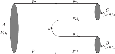
the corresponding amplitude in Fig. 1 can be written as
(1)
Figure 1: The Feynman diagram of two-body open charm strong decay.
Integrating out the momentum with instantaneous approximation,
and neglecting all the negative energy contributions which have very small influence on the amplitude fu ,
then the leading order amplitude Eq.(1) is the overlap integration of the positive BS wave functions for the initial and final states,
(2)
where , and
are the positive BS wave functions of the initial meson , finial meson and , respectively.
.
, ,
are the three dimensions relative momentum between the quark and anti-quark of the initial meson ,
finial meson and , respectively.
,
.
and are the three momentum of finial mesons and .
.
Finally, the two-body open charm strong
decay width of the and charmonium states can be expressed as
(3)
where
which is the three momentum of the final mesons.
III Numerical results and discussions
In order to fix the parameters in Cornell potential in Eq.(11) and masses of quarks,
we take GeV2, GeV,
GeV, GeV, GeV, GeV, GeV, w1 ; mass1 ,
which give the best to fit the mass spectra of the ground charmonium states and other heavy meson states.
The corresponding mass spectra of the -wave charmonium states are shown in Table 1 which are obtained by solving the coupled Salpeter
equations Eq.(10).
Table 1: The Mass spectra of -wave charmonia (unit in MeV) mass1 .
‘Ex.’ means the experimental data from PDG PDG .
First, we study the higher charmonium states with , and ,
and give the two-body open charm strong decay results in Table 2.
The mass MeV is close to the result of the
screened potential model (3842 MeV) th8 and the nonrelativistic potential model (3852 MeV) Godfrey .
Limited by phase space , there is one decay mode for the ,
the corresponding decay channel only includes within the kinematic ranges.
And we also get the total strong decay widths of the : MeV,
which is in accordance with the result of the linear potential quark model (22 MeV) zhaoqiang and the usual model (23 MeV) Swanson .
Belle reported a charmonium-like state ,
and they claimed the seems to be a candidate of
the state 3860 .
The Ref. zhaoqiang studied the strong decays of the as by LP and SP models,
and they gave a similar value MeV.
The analysis of Ref. th5 showed that the was an indication of the state.
Assuming the as the ,
the Ref. x3860zgwang calculated the strong decay of the ,
the total decay of the state ranged from 110
to 180 MeV with GeV-1,
the corresponding decay mode and total decay
width were consistent with the experimental data.
Taking the as the ,
we get the strong decay width MeV,
which is smaller than the center value of the : MeV.
But the strong decay width is related to the parameter in the model,
the result increases with the parameter .
In addition,
considering the large uncertainties of the mass and decay width for the ,
we can’t exclude that the is .
And more investigations are needed to confirm the property of the in the future.
By solving the Eq. (10), we get the mass of as: MeV,
which is close to the result of the screened potential model (4131 MeV) th8 .
The dominant strong decay of the is OZI-allowed two-body open charm strong decay.
And there are two decay types: and ,
while decay mode is forbidden.
Therefore, the final mesons include , and within the kinematic ranges,
and there is no .
The decay channel has the largest phase space,
but due to the node structure of ’s wave functions,
the integrand (which consists of the overlapped wave functions) oscillates accordingly in the amplitude.
The positive contribution of the integrand almost cancels the negative contribution in ,
leading to a smallest value of in Table 2.
So the dominant contribution comes from ,
which is consistent with the result of the screened potential model th8 .
Then we calculate all of the two-body open charm strong decays,
the total strong decay width MeV is close to the result of the unquenched quark model (71 MeV) liuxiang2021 .
The was observed by Belle from
the process 39404160 .
The Ref. th8 and zhao1 discussed possible interpretations for the based on the NRQCD calculations and the potential model, two likely assignments for the were and .
The Ref. x41601 calculated the strong decays of the ,
they found that the explanation of the
as the is possible and the assignment of the as the can not
be excluded.
The Ref. 416011 calculated the strong decay of the which was assumed as the ,
, or by the model,
they thought that the excited charmonium state cannot be ruled out as
an assignment for the .
Considering the as the state, we also calculated the strong decay of the in Ref. 4S4160 ,
the ratio of the decay width of was larger than
the experimental data of the ,
thus,
the was not the candidate of the .
In this work, the mass of is close to the ,
assigning the as the ,
the total strong decay width MeV is rough consistent with the result of experimental
results for : MeV.
Then we calculate relative ratios ,
and ,
both of which agree with the experimental results of by Belle collaboration 39404160 .
Therefore,
is a good candidate for .
III.2 and
Using the BS method, we get the masses and wave functions of the and .
The MeV is close to the result of the nonrelativistic potential model (3925 MeV) Godfrey .
The two-body open charm strong decay results
have been shown in Table 3.
For the , there is only one decay mode ,
so the final state include state.
The corresponding decay width MeV is the same as the results of linear potential quark model (102 MeV) zhaoqiang ,
but smaller than the results of other methods.
The mass MeV is larger than the result of
the screened potential model (4178 MeV) th8 ,
but smaller the than results of the relativized Godfrey-Isgur model (4317 MeV) and nonrelativistic potential model(4271) MeV Godfrey .
The two-body open charm strong decay of have three decay modes:
and include five final states: , , , , .
The dominant strong decay channels are , and .
The ratios between different partial width are independent of the strength parameter ,
they are and
,
which can be explored in the future experiment.
The total strong decay width MeV,
which is similar to the result of the linear potential quark model (23 MeV) and the relativized
Godfrey-Isgur model (39 MeV) Godfrey ,
but smaller than the result of the unquenched quark model (48 MeV) liuxiang2021 .
Table 3: The strong decay type and decay widths of the and (unit in MeV).
The results in the parentheses are calculated with MeV.
Some charmonium-like states with : ,
, have been discovered in experiments PDG .
They may be the good candidates for the .
The Ref. 3872-1 calculated the E1 radiative and strong decays of the as all possible and
states.
The Ref. 3872-2 explored the , and charmonium candidates for , and the , were favored candidates for the , both have prominent radiative decays.
The was examined by the molecule model and the charmonium model in Ref. 3872-3 ,
the author thought that the may fit more
likely to the excited charmonium than to the molecule.
The quantum number of the is the same as ,
but its mass is about 50 MeV lighter than the result of our prediction.
Considering the as the ,
we have calculated the radiative decay widths of the through the BS method in Ref. thwang1 ,
the result was in agreement with the experimental data.
However, there is no two-body open charm strong decay for which has a narrow width MeV PDG .
Because the mass of happens to lie around the threshold,
many authors believed that it’s an ideal candidate for the
exotic hadrons.
Various scenarios have been discussed in the literature Ref. Olsen ; fkguo ; swanson1 ; Ferretti ; slzhu2 ,
but until now, the nature of the still remains unclear,
many more investigations are very essential to understand the property of the in the future.
The Ref. th3 calculated the strong decay of as with MeV, and they got the width MeV.
The Ref. liuxiang2021 gave the decay width of : MeV,
which was consistent with experimental data,
and it was possible to assign as the state.
Considering the as the state,
we calculate its strong decays by the BS method.
The total strong decay width MeV is larger than 29.7 MeV with MeV,
so the strong decay width is sensitive to the mass of the .
The total strong decay width MeV is agreement with
the world average data MeV PDG .
Therefore,
the is a good candidate for the state.
Assigning the as the ,
the relative ratios are
and
,
which can provide more useful information to observe the in the future experiment.
Table 4: The strong decay type and decay widths of the and (unit in MeV).
The results in the parentheses are calculated with MeV and MeV.
By solving the Eq.(10),
we also obtain the mass of and ,
the MeV is in accordance with the
relativized Godfrey-Isgur model (3979 MeV) and the nonrelativistic potential model (3972 MeV) Godfrey .
The MeV is smaller than the mass in the
relativized Godfrey-Isgur model (4337 MeV) and the nonrelativistic potential model (4317 MeV) Godfrey .
The two-body open charm strong decays of the and ,
are shown in Table 4.
The state has two decay modes: ,
and the corresponding final states include , and .
We find that the dominant channels are and ,
the is very small
with the small phase space.
Then the total strong decay width MeV,
which is smaller than the results of the nonrelativistic potential model (80 MeV) Godfrey and the usual model (60.5 MeV) Swanson .
There are three decay modes for the : ,
and six strong decay channels , ,
,, and .
The total strong decay width MeV is consistent with the results of
linear potential quark model (43 MeV) and screened potential quark model (30 MeV) zhaoqiang .
is the dominant decay channel,
which contribute about of the total strong decay width.
We also predict the relative ratios
and with MeV.
The Ref. th11 studied the strong decays of the and ,
the mass of was very close to the experimental data of the ,
but the decay width MeV,
which was 3 times that of the experimental value.
The was assigned to the ,
and the strong decay width was MeV in the Ref. 39301 .
Assigning the as the ,
we have taken two methods to calculate the OZI-allowed two-body strong
decay processes of the state in detail: the BS method and the extended model in Ref. thwang .
The total decay width is consistent with the experimental data,
which means the is a good candidate for the ,
so we only list the total strong decay width of the in this paper.
The was observed by Belle in the mass spectrum,
which is a candidate for the 4350 .
The open-charm decay of with GeV-1
was well consistent with experimental data of the ,
which showed that the
as a good candidate of in Ref. th13 .
Assigning
the as the state,
the Ref. zhaoqiang studied its the strong decay,
and got the decay width which was about 90 MeV.
Considering the as the ,
some new decay channels are allowed with the increasing mass,
such as , , and .
So the total decay width increases to MeV,
which is consistent with the results of the nonrelativistic potential model (66 MeV) Godfrey ,
but larger than the result of experimental dada MeV.
Thus, if one takes the as an assignment of the ,
the precision measurements are needed in further experiments.
The relative ratios
and with MeV,
also can provide evidence to discover the for the future experiment.
Table 5: The strong decay type and decay widths of the and (unit in MeV).
Finally, we study the higher charmonium states with , and .
The MeV is consistent with the mass of
the relativized Godfrey-Isgur model (3956 MeV) and the nonrelativistic potential model (3934 MeV) Godfrey .
The MeV is close to the results of the nonrelativistic potential model (4279 MeV) Godfrey .
And the two-body open charm strong decay results
are shown in Table 5.
The has one decay mode , and only can decay into .
The total strong decay width MeV,
which is smaller than the results of other theoretical models.
The main decay modes of the include .
The final states , , , , are allowed.
The total strong decay width MeV is in accordance with the result of the screened potential quark model (30 MeV) zhaoqiang .
The main decay channel contributes about of the total strong decay width.
The corresponding relative ratios:
and
can provide theoretical
assistance to confirm the in future experiments.
IV summary
In conclusion, we have studied the two-body open charm strong decays of the
and charmonium states by the BS method combined with the model.
The wave functions and mass spectra of the initial and charmonium states are obtained
by solving the BS equation with the relativistic correction.
Considering the relativistic correction,
the masses of some charmonium states in our model will have a difference with the results of the nonrelativistic potential model.
Then we get the two-body open charm strong decay widths of the and charmonium states.
Considering the as ,
the narrow strong decay width is smaller than the experimental data,
because the strong decay width depend on the parameter,
and there are large errors in the mass and the width of the ,
we cannot rule out that the is .
Taking the as the ,
the total strong decay width is in accordance with the experimental
result of the with the uncertainty.
In addition, because of the node structure of the ’s wave functions,
the integrand oscillates accordingly in the amplitude,
the decay is strong suppressed.
Then the relative ratios ,
and are consistent with the experimental results.
Therefore, the is a good candidate for the .
Assigning the as the ,
we find that the total strong decay width is in agreement with the data of the ,
so the resonance is a good candidate for the .
The relative ratios and
can provide
useful information in experiments.
The has been confirmed as the state in our previous work,
so we only show the strong decay width in this work.
Considering the as ,
we find that the total strong decay width of the is larger than the result of the ,
thus, if we take the as an assignment of the ,
we need many more investigations in the future.
Finally,
we also calculate the two-body open charm strong decay of the and ,
and give the total strong decay widths of the and .
The corresponding relative ratios
and can
give the theoretical
assistance in future experiments.
Acknowledgements
We would like to thank Shi-Lin Zhu for many valuable
discussions and assistance during this work.
This work was supported by
the National Natural Science Foundation of China (NSFC) under
Grant No. 11865001 and No. 12075073,
and the CAS ”Light of West China” Program.
Appendix A Instantaneous Bethe-Salpeter Equation
The BS equation which is used to describe the heavy mesons can be written as BS :
(4)
where and are the wave function and the momentum of the bound state, respectively.
is the relative momentum between quark and anti-quark in meson,
,
and , are the momentum and the mass of the quark and anti-quark, respectively.
The is the
interaction kernel between the quark and antiquark.
In order to solve the Eq. (4),
the instantaneous approximation is adopted in the interaction kernel Salp :
For convenience, the relative momentum is decomposed into two parts
and ,
is related to three dimensional BS wave function as
follows:
(6)
and are the propagators of the quark and anti-quark which can be decomposed as:
(7)
with
(8)
where for quark and anti-quark, respectively,
and
.
The positive and negative energy projected wave functions are defined as:
(9)
Then under instantaneous approximation,
with contour integration over on both sides of
Eq. (5), we obtain the full Salpeter equation:
(10)
The wave functions are different for the bound states with different quantum (or ).
First, we give the original BS wave functions for the different bound state, then reduce the wave functions through the last
equation of Eq. (10). Finally the numerical result of the wave functions and mass spectrum are obtained
by solving the first and second equations in Eq. (10).
And the detailed solution of the Salpeter equation also has been discussed in Ref. w1 ; BS1 ; glwang ; mass1 .
To solve the Eq. (10), we take the Cornell
potential as the instantaneous interaction kernel ,
which include a linear scalar interaction and a vector interaction.
In the momentum space and the C.M.S of the bound state,
the interaction potential is read as:
(11)
where is the string constant and is the running coupling constant. In order to fit the data of
heavy quarkonia, a constant is often added to confining
potential. We also introduce a small
parameter to
avoid the divergence in the denominator. The constants , , and
are the parameters that characterize the potential.
Appendix B The relativistic wave functions
In this paper, we focus on the OZI-allowed two-body open charm strong decay of the and charmonium states.
The detailed wave functions have been obtained in Refs. w1 ; mass1 ; BS1 ; glwang .
We mainly introduce the relativistic BS wave functions of the ,
, and in this section.
B.1 The relativistic BS wave function of the with
The original BS wave functions of the with can be written as
(12)
where is the mass of bound state ,
is the original radial wave functions that are related to .
Taking Eq. (12) to Eq. (10),
the relativistic BS wave functions and the mass
spectrum can be obtained by solving the Salpeter equations Eq. (10).
Then the relativistic positive BS wave function is shown as,
(13)
The corresponding coefficients are
where and
are
the masses and the energies of the
quark and anti-quark in the state.
B.2 The relativistic BS wave function of the with
The original BS wave functions of the with is constructed by ,
and the polarization vector ,
(14)
where is the polarization vector of the axial vector meson.
The corresponding relativistic positive BS wave function is obtained in Eq. (15) by solving the Eq. (10),
(15)
B.3 The Relativistic BS Wave function of the with
The original BS wave function of the is constructed by , ,
the polarization tensor and the gamma matrices,
where is the polarization tensor of the with .
According to the solve the Eq. (10),
we get the relativistic positive BS wave function,
where the coefficients are
B.4 The Relativistic BS Wave function of the with
The original BS wave functions of the with also is constructed by ,
and the polarization vector ,
(18)
where is the polarization vector of the .
The corresponding relativistic positive BS wave function is obtained in Eq. (15) by solving the Eq. (10),
(19)
where the coefficients are
References
(1)
S. K. Choi , Belle Collaboration, 91, 262001(2003).
(2)
P. Pakhlov , Belle Collaboration, 100, 202001(2008).
(3)
T. Aaltonen , CDF Collaboration, 102, 242002(2009).
(4)
T. Aaltonen , CDF Collaboration, A 32(26), 1750139(2017), arXiv:1101.6058 [hep-ex].
(5)
R. Aaij , LHCb Collaboration, 118, 022003(2017).
(6)
R. Aaij , LHCb Collaboration, D 95, 012002(2017).
(7)
M. Tanabashi ., (Particle Data Group), D 98, 030001(2018).
(8)
B. Aubert , BABAR Collaboration, D 81, 092003(2010).
(9)
X. Liu, 59, 3815(2014).
(10)
H. X. Chen, W. Chen, X. Liu and S. L. Zhu 6391, (2016).
(11)
C. P. Shen Belle Collaboration, 104, 112004(2010).
(12)
K. Chilikin , Belle Collaboration, D 95, 112003(2017).
(13)
D. Y. Chen, C 76, 671(2016).
(14)
H. X. Chen, E. L. Cui, W. Chen, X. Liu and S. L. Zhu, C 77, 160(2017).
(15)
W. Chen, and S. L. Zhu, D 83, 034010(2011).
(16)
J. Ferretti, E. Santopinto, M. Naeem Anwar and Y Lu, C 80, 464(2020).
(17)
H. F. Fu and L. B. Jiang, C 79, 460(2019).
(18)
M. X. Duan, S. Q. Luo, X. Liu and T. Matsuki, D 101, 054029(2020).
(19)
D. Y. Chen, X. Liu and T.Matsuki , 043B05 4(2015).
(20)
B. L. Huang, Z. Y. Lin and S. L. Zhu, D 105, 036016(2022).
(21)
C. R. Deng, H. Chen and J. L. Ping, D 103, 014001(2021).
(22)
G. L. Yu, Z. G. Wang and Z. Y. Li, C 42, 043107(2018).
(23)
X. Liu, Z. G. Luo and Z. F. Sun, 104, 122001(2010).
(24)
L. C. Gui, L. S. Lu, Q. F. Lu, X. H. Zhong and Q. Zhao, D 98, 016010 (2018).
(25)
W. Chen, H. X. Chen, X. Liu, T. G. Steele and S. L. Zhu, D 96, 114017(2017).
(26)
T. Barnes, S. Godfrey and E. S. Swanson, D 72, 054026 (2005).
(27)
M. X. Duan and X. Liu,D 107, 074010 (2021).
(28)
E. S. Swanson, , 429 243(2006).
(29)
B. Q. Li and K. T. Chao D 79, 094004(2009).
(30)
T. Branz, R. Molina aand E. Oset, D 83, 114015(2011).
(31)
V. Kher and A. K. Rai, C 42 083101(2018).
(32)
Z. H. Wang, Y. Zhang, T.H. Wang, Y. Jiang and G. L. Wang, C 80, 791(2020)
(33)
Z. H. Wang, Y. Zhang, L. B. Jiang, T. H. Wang Y. Jiang and G. L. Wang,
C 77, 1:43 (2017).
(34)
T. H. Wang and G. L. Wang B 697 233 (2011).
(35)
T. H. Wang, G. L. Wang, Y. Jiang and W. L. Ju G 40 035003(2013).
(36)
T. H. Wang, G. L. Wang, H. F. Fu and W. L. Ju, ,07, 120(2013).
(37)
L. Micu B 10, 521(1969).
(38)
Z. F. Sun and X. Liu D 80, 074037(2009).
(39)
J. Segovia, D. R. Entem and F. Fernndez D 715, 322(2012).
(40)
H. F. Fu, X. J. Chen, G. L. Wang and T. H. Wang A 27, 1250027(2012).
(41) C. S. Kim, G. L. Wang, B, 584, 285(2004).
(42)
C. H. Chang and G. L. Wang, G, 53, 2005(2010).
(43)
F. K. Guo and U. G. Meißner, D 86, 091501 (2012).
(44)
G. L. Yu and Z. G. Wang C 42, 043107(2018).
(45)
K. T. Chao, B 661, 348(2008).
(46)
H. Wang, Z. Z. Yan and J. L. Ping, C 75 196(2015).
(47)
Y. C. Yang, Z. R. Xia and J. L. Ping, D 81 094003(2010).
(48)
T. Barnes and S. Godfrey, D 69 054008(2004).
(49)
E. J. Eichten, K. Lane and C. Quigg, D 69 094019(2004).
(50)
M. Suzuki, D 72 114013(2005).
(51)
S. L. Olsen, 10 121(2015).
(52)
F. K. Guo, C. Hanhart, U. G. Meißner, Q. Wang, Q. Zhao and
B. S. Zou 90 015004(2018).
(53)
R. F. Lebed, R. E. Mitchell and E. S. Swanson 93 143(2017).
(54)
J. Ferretti, G. Galat and E. Santopinto, D 90 054010(2014).
(55)
L. Meng, G. J. Wang, B. Wang and S. L. Zhu, D 104 094003(2021).
(56)
H. Wang, Y. C. Yang and J. L. Ping, A 50, 76(2014).
(57)
P. G. Ortega, J. Segovia, D. R. Entem and F. Fernndez, B 778 1-5(2018).
(58) E.E. Salpeter and H.A. Bethe, Phys. Rev, 84, 1232(1951).
(59) E.E. Salpeter, Phys. Rev, 87, 328(1952).
(60)
C. H. Chang, J. K. Chen and G. L. Wang, , 46, 467(2006).